Exploring Zero-Shot Foundation Models for Multivariate Time Series Anomaly Detection
July 14, 2026
Abstract
mtsad is essential for reliability and safety in domains such as industrial process monitoring and financial risk management, yet conventional approaches rely on application-specific models that are costly to train and hard to scale. fms, pre-trained on broad data with strong zero-shot generalization, have recently become available for univariate time series forecasting, raising the question of whether they can address mtsad without task-specific training. We investigate the zero-shot application of a univariate forecasting fm, TimesFM, to industrial mtsad on the swat benchmark, evaluating two strategies: treating the fm as a per-feature forecaster with thresholded prediction errors, and as an embedder whose intermediate representations feed standard outlier detectors. Neither of our proposed setups is competitive with established baselines; embeddings reveal only partial separation between normal and anomalous segments, insufficient for reliable detection. The cause is that the fm is too effective at capturing temporal dynamics, yielding low error even within fully anomalous windows, so persistent anomalies become indistinguishable from normal behavior. However, these observations yield valuable insights: the error peaks at anomaly boundaries, indicating fms reliably detect distribution changes. We conclude that the proposed naive zero-shot fms are unsuitable for mtsad but promising for change-point detection.
1 Introduction↩︎
mtsad plays a vital role in ensuring the reliability and safety of numerous application domains, including industrial process monitoring, predictive maintenance, fraud detection, and cybersecurity [1]. The recorded data in these settings is typically high-dimensional, noisy, and strongly imbalanced, as anomalous events are rare and heterogeneous. Consequently, detection is commonly addressed by models tailored to a specific application and dataset — an approach that is costly to develop, energy-intensive to retrain, and difficult to scale across environments or distribution shifts.
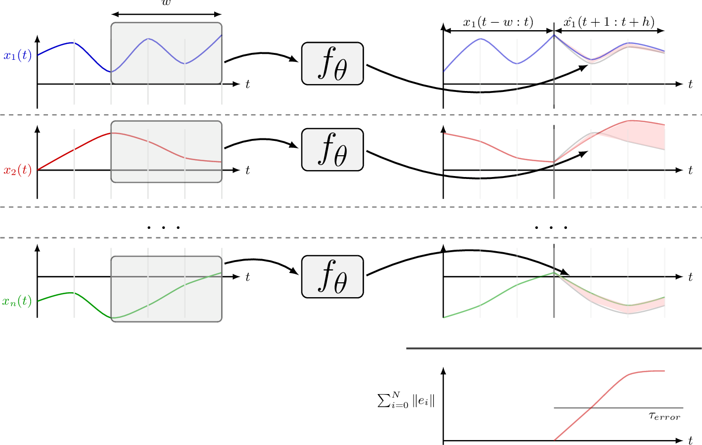
Forecasting-based methods are among the most widely adopted paradigms for mtsad [1]. A model \(f_\theta\) is trained to predict future observations from a context window, e.g. \(\hat{X}_{t+1} = f_\theta(X_{t-w:t})\), and anomalies are flagged when the prediction error \(e_{t} = \| \hat{X}_{t+1} - X_{t+1} \|\) exceeds a threshold. The model must be trained on in-distribution data, however, which perpetuates the per-dataset specialization problem.
fms — large models pre-trained on broad, diverse data through self-supervision — offer a potential escape from this cycle [2]. They have demonstrated strong zero-shot performance across many domains, and dedicated univariate time series fms have recently become available [3]. Applying such a model directly to mtsad would eliminate the need for dataset-specific training while leveraging representations learned from large-scale temporal data. Despite this appeal, the zero-shot application of fms to industrial mtsad remains largely unexplored.
We therefore investigate: Can a zero-shot univariate time series fm detect anomalies in industrial multivariate time series without any task-specific training? We make the following contributions:
We propose and evaluate two complementary zero-shot strategies for applying a univariate forecasting fm to mtsad: using it as a per-feature forecaster with thresholded prediction errors, and as an embedder whose intermediate representations feed a standard outlier detector.
We show that neither strategy is competitive with established baselines on the swat benchmark, and identify the root cause: the fm adapts to anomalous dynamics just as effectively as to normal behavior, making persistent anomalies indistinguishable from normal operation.
We identify change-point detection as a more suitable use case, supported by the observation that forecasting error peaks reliably at anomaly boundaries even in the zero-shot regime.
Related Work↩︎
Classical forecasting-based mtsad methods achieve strong performance by training directly on the target domain, but at the cost of requiring dataset-specific optimization [1]; in contrast, we study whether a pretrained, zero-shot fm can offer comparable detection capability without any such task-specific training.
Early work on applying fms to time series anomaly detection focused on univariate settings, as surveyed by [4]. The zero-shot transfer of fms to mtsad has been explored on standard benchmarks such as SMAP and MSL [5]. More recently, ChronosAD [6] demonstrated that using Google’s Chronos fm as a feature extractor yields promising results across an extensive collection of mtsad benchmarks, establishing fms as a competitive approach when used in a representation-learning role.
2 Background↩︎
2.1 Multivariate Time Series Anomaly Detection↩︎
We denote by \(\mathbf{X} \in \mathbb{R}^{T\times C}\) a multivariate time series with \(T\) time steps and \(C\) channels (variates). The time steps are indexed by \(t \in \{ 1, \ldots, T\}\) with a corresponding label \(y \in \{0,1 \}^T\) indicating benign (\(y_t=0\)) or anomalous behaviour (\(y_t=1\)). The goal of unsupervised mtsad is to identify anomalous observations \(\mathbf{x}_t \in \mathbb{R}^C\) at each time step \(t\), based on the joint temporal behavior across multiple channels. This is in contrast to univariate anomaly detection, which only considers a single channel in isolation.
The procedure of unsupervised mtsad typically involves two steps: first, a model is trained on the multivariate time series data to learn a representation of behavior under a benign regime. This model can then be leveraged to identify anomalous observations based on deviations from the learned representation of normal behavior. Classical approaches to mtsad include reconstruction-based methods, such as autoencoders, and forecasting-based methods [1]. More recently, deep learning-based methods have been proposed, which leverage the ability of neural networks to capture complex temporal dependencies and cross-channel correlations [7].
To benchmark the performance of mtsad methods, several datasets from different domains have been proposed, including NASA telemetry data [8], server machine data [9], [10], water treatment plant data [11], [12], and more recently, the qad benchmark [13], which provides a collection of multivariate time series data from a real-world industrial system under various operating conditions and fault scenarios. An example of a multivariate time series for anomaly detection is illustrated in 1, showing two selected variates from a trace taken from the qad benchmark [13]. This dataset is not used in this work; however, thanks to its periodic behavior, it nicely illustrates the anomalies.
![Figure 1: Illustration of anomalies on the qad on two selected features: A multivariate signal is monitored over time and anomalies (highlighted in red) are identified from deviations of the joint temporal behavior across multiple channels rather than from a single variable in isolation. Illustration adapted from [13].](/article/2607.12454/img/mts.png "fig:")
2.2 Foundation Models↩︎
fms are a class of machine learning models that are trained on large-scale datasets and can be adapted to a wide range of downstream tasks. The most prominent fms are Large Language Models, which have achieved remarkable success in natural language processing, but fms have also been applied to other modalities, such as image, audio, and video. Although the term fm is not restricted to a specific architecture [2], the Transformer architecture has become the de facto standard for fms [4].
Formally, we define a univariate time series fm as a function \(f_\theta: \mathbb{R}^{w} \to \mathbb{R}^h\) that maps an input sequence \(x_{t-w:t}\) of context window length \(w\) to an output sequence \(\hat{x}_{t+1 : t+1+h}\) of the horizon length \(h\), where \(\theta\) are the pretrained parameters of the model.
To make it more generic, we decompose the fm \(f_\theta\) into \[f_\theta = \phi_\theta \circ g_\theta\] an encoder \(g_\theta: \mathbb{R}^{w} \to \mathbb{R}^d\) that maps the input sequence to a latent representation \(v\in \mathbb{R}^d\) and a decoder \(\phi_\theta: \mathbb{R}^d \to \mathbb{R}^h\) that maps the latent representation to the output sequence.
This work focuses on the application of univariate time series fms only [3], although multivariate time series fms are becoming more common, where cross-channel dependencies are explicitly modeled or each variate is treated as a separate channel in a multivariate time series [4]. However, recent works suggest that treating each channel independently suffices for mtsad on published benchmarks [14]–[16].
3 Methodology↩︎
For this exploratory work, we consider two ways of leveraging a univariate time series fm for multivariate time series anomaly detection, which are detailed in the following. For both approaches, we use a pretrained univariate time series fm \(f_\theta\) trained to predict the next \(h\) time steps of a univariate time series given a context window of length \(w\).
3.1 Forecasting-Based Anomaly Detection↩︎
Similar to classical forecasting-based anomaly detection methods [17], [18], we can leverage a univariate time series fm to predict future values of each channel in a multivariate time series. Here we intentionally omit the cross-channel dependencies and treat each channel independently, which allows us to use a univariate fm for multivariate time series anomaly detection. Although this approach does not capture the cross-channel dependencies, recent works suggest that cross-channel dependencies are not critical for anomaly detection on published benchmarks [14]–[16].
As illustrated in 2, we detect anomalies by comparing the predicted future values \(\hat{X}_t\) with the observed future values \(X_t\). For each time step \(t\), we compute a joint prediction error \(e_t\) by aggregating the per-channel errors \(e_{c,t} = \| \hat{X}_{c,t} - X_{c,t} \|\) over all channels, \[e_t = \sum^{C}_{c=1} e_{c,t}.\] To identify anomalous observations, the prediction error is then thresholded against a predefined value \(\tau_{error}\) \[\hat{y}_t = \mathbb{I}(e_t > \tau_{error}),\] where \(\hat{y}_t\) is the predicted label for time step \(t\) and \(\mathbb{I}\) is the indicator function.
3.2 Embedding-Based Anomaly Detection↩︎
In contrast to the forecasting-based approach, we can also leverage the latent representations of a univariate time series fm for anomaly detection. Here, we use the encoder \(g_\theta\) of the fm to map each channel of a multivariate time series to a latent representation \(v_{c,t} \in \mathbb{R}^d\) for each channel \(c\) and time step \(t\). These per-channel representations serve as input features for a downstream anomaly detection method. The latent representations of all channels are then concatenated to form a joint embedding vector \(z_t \in \mathbb{R}^{C \cdot d}\) for the multivariate observation at time step \(t\). This joint-embedding vector can then be used as input to a downstream anomaly detection method, such as an if [19], to identify anomalous observations based on their distance to the learned representation of normal behavior. The overall procedure of extracting the joint embedding vector is illustrated in 3.

Following the standard procedure of unsupervised anomaly detection methods, we can then use the joint-embedding vectors \(z_t\) to train an if on the normal operating regime of the system and use it to identify anomalous observations based on their distance to the learned representation of normal behavior.
4 Experiments & Results↩︎
4.0.0.1 Experimental Setup.
For all experiments, we use TimesFM [3] (version 1.2.0) via its publicly available implementation1 as the univariate time series fm. TimesFM is a Transformer-based model pretrained on a large corpus of univariate time series data from various domains. Although it is possible to fine-tune the model on the target domain, we explicitly focus on the zero-shot regime in this work, where the pretrained model is directly applied to the target domain without any further training or adaptation.
We use a context length of \(w=100\), consistent with related work [20], and a forecast horizon of \(h=32\), chosen as a trade-off between TimesFM’s long-horizon forecast capability and per-step prediction accuracy. All experiments are conducted on a single NVIDIA GeForce RTX 3090 with 24 GB of VRAM and an Intel(R) Core(TM) i9-10980XE CPU @ 3.00GHz.
4.0.0.2 Datasets.
We evaluate the proposed approaches on the swat benchmark [12], which is a publicly available dataset that contains multivariate time series data from a real-world water treatment plant under various operating conditions and fault scenarios. The dataset contains 51 channels and a total of 11 days of data, with 7 days of normal operation and 4 days of anomalous operation. The dataset is split into a training set of 7 days and a test set of 4 days, with the anomalous operation occurring in the test set. The dataset is preprocessed by normalizing each channel to have zero mean and unit variance, and by removing any missing values.
4.0.0.3 Metrics.
We evaluate the performance of the proposed approaches using the F1 score, which is a commonly used metric for anomaly detection that balances precision and recall. The threshold \(\tau_{error}\) for the prediction error in the forecasting-based approach is optimized on the test set to maximize the F1 score.
4.1 Qualitative View on Forecasting-Based Anomaly Detection↩︎
4 illustrates the per-channel and aggregated prediction error on a representative excerpt of the swat dataset.
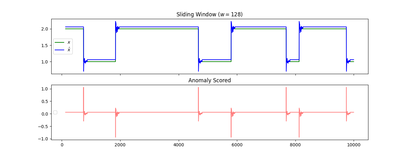
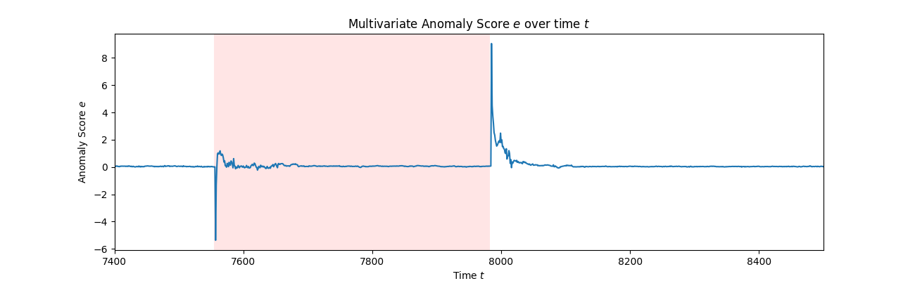
Figure 4: Anomaly scoring on the swat dataset using per-channel forecasts from a fm, with per-channel errors summed into a joint score.. a — Exemplary forecast on a representative channel with its per-channel error profile on benign data; sharp transitions in the signal cause transient error spikes even in the normal regime., b — Aggregated multivariate score profile over a window containing an anomalous segment; the score spikes at the entry and exit boundaries but collapses to near zero throughout the anomaly itself.
As shown in 4 (a), the fm reconstructs the benign signal accurately, keeping the prediction error consistently low. The quantitative results are correspondingly poor, with an F1 score close to zero, confirming that the forecasting-based approach fails to detect persistent anomalies.
The multivariate score profile in 4 (b) reveals the underlying cause. The prediction error is low during benign operation, spikes sharply at the transitions into and out of the anomalous region, but returns to near zero throughout the anomaly itself. This spike is transient: it persists only while the sliding window of length \(w\) straddles the boundary; once the window lies entirely within the anomalous segment, the fm adapts to the new dynamics and the score collapses. The model is therefore too effective at capturing temporal structure — it tracks anomalous behavior just as faithfully as normal behavior, rendering persistent anomalies indistinguishable from normal operation. Error peaks at anomaly boundaries do, however, make the fm a natural candidate for change-point detection.
4.2 Embedding-Based Anomaly Detection↩︎
We apply the encoder \(g_\theta\) independently to each variate and, for each channel, concatenate the intermediate representations from all transformer blocks into a single feature vector. These per-channel vectors are then concatenated across channels to form the joint embedding \(z_t\) per time step, as described in 3.2. An if is trained on embeddings from the normal operating regime and used to score the test set.
5 shows the embeddings extracted from the wadi benchmark [11], projected to three dimensions via PCA. Normal and anomalous embeddings form partially overlapping clusters, suggesting that the fm encodes some structure correlated with the operating regime, though the separation is not pronounced enough for reliable detection in the full embedding space.

1 reports F1 scores on the swat benchmark. The proposed TimesFM + if pipeline achieves an F1 of 0.480, well below all baselines — including simple heuristics such as L2-norm (0.782) and the best-performing method, PCA Error (0.833).
| Method | SWaT |
|---|---|
| Random | 0.218 |
| Sensor range deviation | 0.231 |
| L2-norm | 0.782 |
| 1-NN distance | 0.782 |
| PCA Error | 0.833 |
| 1-Layer MLP | 0.771 |
| Single block MLPMixer | 0.780 |
| Single Transformer block | 0.787 |
| 1-Layer GCN-LSTM | 0.829 |
| TimesFM + if | 0.480 |
6pt
The large gap to even the simplest baselines indicates that zero-shot embeddings from a univariate forecasting fm do not provide a sufficiently discriminative representation for downstream anomaly detection on industrial data. This is consistent with the qualitative observation in 5: although some cluster structure is visible in the projected space, the embeddings of normal and anomalous segments overlap substantially, leaving the if unable to separate them reliably.
5 Discussion & Future Work↩︎
Both strategies fail for the same underlying reason, but it is not the one intuitively expected: the fm does not lack domain knowledge — it generalizes too well. In the forecasting-based approach, the model adapts to anomalous dynamics within a single sliding window, keeping the prediction error low even deep inside an anomalous segment. In the embedding-based approach, the same adaptability causes normal and anomalous segments to produce overlapping representations. The core issue is therefore not a failure to generalize, but a failure to specialize: a model pre-trained for accurate forecasting optimizes for reconstruction fidelity rather than anomaly sensitivity, and those two objectives are fundamentally at odds for persistent anomalies.
This distinction is reflected in the baseline comparison: PCA Error, the strongest baseline in 1, fits a single global subspace of normal behavior over the entire training set, whereas the fm re-adapts locally within each sliding window. A persistent anomaly therefore remains a persistent outlier with respect to a fixed global model, while it is gradually absorbed into the fm’s local forecast.
This negative result stands in contrast to ChronosAD [6], which reports strong performance using embeddings from a different fm (Chronos) as a feature extractor across a broad collection of mtsad benchmarks. We see several possible explanations for this discrepancy, which we cannot yet disambiguate from our results alone. First, Chronos and TimesFM differ in architecture and pretraining corpus, and may therefore encode different inductive biases with respect to anomaly-relevant structure. Second, ChronosAD evaluates across a wide range of benchmarks, whereas our embedding analysis is limited to swat only; it is possible that our chosen datasets are simply less favorable to this representation-based approach. Third, downstream detector choice may matter: we pair embeddings with a single Isolation Forest, while ChronosAD’s pipeline may use a different or better-tuned scoring method. Disentangling these factors — fm choice, benchmark choice, and detector choice — is an important direction for future work.
This boundary-sensitivity property points to a more appropriate use case. Because the forecasting error spikes sharply at the transitions into and out of anomalous segments (4), the fm reliably signals distributional changes even in the zero-shot regime. This makes it a natural candidate for change-point detection, a related but distinct task from anomaly detection, where the goal is to locate the onset of a regime shift rather than to label every anomalous time step.
5.0.0.1 Future Work.
Fine-tuning the fm on target-domain data, or even a few-shot adaptation, could shift the model toward anomaly sensitivity by exposing it to domain-specific normal behavior. A complementary direction is to replace the univariate fm with a genuinely multivariate one that explicitly models cross-channel dependencies. Although current benchmarks show limited benefit from cross-channel modeling in MTSAD [15], real-world industrial systems often exhibit strong inter-sensor correlations that a multivariate fm could exploit. Finally, the boundary-detection property observed here suggests that fms may support root cause analysis [21]: by identifying which channels exhibit the sharpest error spike at a transition, one could localize the origin of a fault without any task-specific training.
5.0.0.2 Limitations.
The main limitation of this work is its narrow experimental scope: we evaluate a single univariate fm on a single benchmark dataset, which constrains the generalizability of our conclusions. We further restrict our study to the zero-shot regime; performance may differ substantially under few-shot or fine-tuning settings. Likewise, we pair the fm with a single class of downstream anomaly detectors, leaving open whether other detection methods would yield different results. Finally, our setup assumes regularly sampled time series and does not address the sparse, irregularly sampled data frequently encountered in industrial practice [20].
6 Conclusion↩︎
In this work, we investigated whether univariate time series fms can be applied to mtsad in a zero-shot regime, without any task-specific training. Using TimesFM on the swat benchmark, we evaluated two complementary strategies: employing the fm as a per-feature forecaster with thresholded prediction errors, and as an embedder whose intermediate representations feed standard outlier detectors. Our results show that neither strategy is competitive with established baselines. The qualitative analysis attributes this to the fm being too effective at capturing temporal dynamics: it produces low forecasting error even within fully anomalous windows, rendering persistent anomalies indistinguishable from normal behavior.
At the same time, this very property suggests a more promising use case. Since the forecasting error peaks at the transitions into and out of anomalous segments, fms reliably respond to changes in the underlying data distribution, making them strong candidates for change-point detection rather than for detecting persistent anomalies.
Future work should explore fine-tuning the fm on target-domain data to overcome the limitations of the zero-shot regime, evaluate genuinely multivariate fms that capture cross-channel dependencies, and extend the analysis to a broader range of benchmarks and downstream detection methods. Investigating the use of fms for change-point detection and root-cause analysis constitutes a further promising direction.
6.0.1 ↩︎
The financial support by the Austrian Federal Ministry of Economy, Energy and Tourism, the National Foundation for Research, Technology and Development and the Christian Doppler Research Association is gratefully acknowledged.
6.0.2 ↩︎
The authors have no competing interests to declare that are relevant to the content of this article.