Abstract
Mixed precision algorithms can significantly enhance the performance of linear algebra solvers by leveraging increasingly powerful low precision hardware while recovering working precision accuracy through, for example, iterative refinement. In this paper, we propose a novel mixed precision algorithm for computing matrix square roots. Our algorithm combines a Schur decomposition approach in low precision with iterative refinement performed through an approximate Newton method. We perform a detailed convergence analysis of the approximate Newton method. For the special case of symmetric positive definite matrices, this analysis implies that one can recover full working precision accuracy under mild conditions. Numerical experiments on x86-64 architectures indicate that our algorithm frequently reduces execution time compared with a fixed working-precision Schur algorithm.
Matrix square root, matrix function, mixed precision computation, iterative refinement, Newton method
65F60, 65F45, 64G50
1 Introduction↩︎
Matrix functions represent an important subject in numerical linear algebra, and their computation has long sparked great interest within the scientific computing community, with applications in control theory, physics, and engineering. A common and crucial matrix function is the matrix square root. Given a matrix \(A\in\mathbb{C}^{n\times n}\) with no eigenvalues on the non-positive real axis \(\mathbb{R}_{\leq 0}\), the (principal) matrix square root \(A^{1/2}\) of \(A\) is the unique matrix \(X \in\mathbb{C}^{n\times n}\) such that \(X^{2}=A\) and all eigenvalues of \(X\) are in the open right-half complex plane.
Direct methods for computing matrix square roots are usually derived from the Schur–Parlett algorithm, often simply referred to as the Schur algorithm; see [1]. It starts by computing a Schur decomposition \(A=QTQ^{*}\), where \(T\) is an upper triangular matrix, and then uses a back-substitution procedure to compute \(T^{1/2}\) from \(T\). The square root is obtained via \(A^{1/2}=QT^{1/2}Q^{*}\). The Schur algorithm is the most widely used method for computing matrix square roots, owing to its favorable numerical stability properties [1].
Matrix iterations such as \[\label{eq:Newton} X_{k+1}=\frac{1}{2}(X_{k}+AX_{k}^{-1}),\qquad X_{0}=A\tag{1}\] represent another popular way to compute matrix square roots; see [1]. Iteration 1 is obtained from applying the Newton method to the matrix equation \(X^{2}-A=0\) and using the commutativity of the iterates \(X_{k}\) with \(A\) to simplify the correction equation. For an overview and analysis of matrix iterations for computing matrix roots, we refer to [1], [2] and the references therein.
Mixed precision computation bears a long and rich history in numerical linear algebra. Traditional mixed precision algorithms, such as classical iterative refinement [3], were originally introduced to enhance the accuracy of potentially numerically unstable algorithms. In contrast, modern mixed precision algorithms are primarily performance driven. They strategically employ lower precision computation to reduce execution time, and use higher precision computation to recover the lost accuracy. A typical way is to use lower precision computation to attain an approximate solution, and then carry out iterative refinement in working/higher precision.
Mixed precision techniques have by now been applied to a broad range of problems in numerical linear algebra [4]. For example, algorithms for solving linear systems have been discussed in [5]–[7], while algorithms for linear least squares problems and their variants are covered in [8]–[10]. A modular framework for the backward error analysis of GMRES is presented in [11]. For eigenvalue and singular value problems, iterative refinement techniques have been developed in [12]–[16] for the symmetric case and in [17] for the nonsymmetric case. Algorithms for computing matrix functions in arbitrary precision have been investigated in [18], [19]. In the context of matrix functions, mixed precision has so far mainly been used to reduce the cost for attaining high accuracy and increase numerical robustness; see [20], [21] for examples.
In this work, we will develop and analyse novel mixed precision algorithms for computing the matrix square root \(X=A^{1/2}\). The general idea is to first compute an approximation \(X_{0}\) in lower precision, and then refine it via iterative refinement to attain the working precision accuracy. It is important to note that 1 is not suited for this purpose. Due to the violation of the commutativity assumption used in deriving this iteration, the error of this method usually stagnates on the level of the lower precision. This limitation can be overcome by going back to the (true) Newton method applied to \(X^{2}-A=0\). This comes at a cost; the correction equation becomes a matrix Sylvester equation, which needs to be solved in every step. We will mitigate this by freezing the Jacobian (leading to an approximate Newton method), using lower precision for solving the correction equation, and reusing the Schur decomposition from computing \(X_{0}\).
The remainder of this paper is structured as follows. In Section 2, we outline the development and later propose mixed precision algorithms for computing matrix square roots. In Section 3, we perform a detailed analysis to demonstrate the convergence and accuracy of the proposed methods. We extend our mixed precision computation framework to matrix \(p\)th roots in Section 4. Numerical experiments are provided in Section 5 to demonstrate the accuracy and efficiency of our mixed precision algorithms.
In this paper, we let \(\lVert A\rVert_{2}\) and \(\lVert A\rVert_{\mathsf F}\) denote the \(2\)-norm and the Frobenius norm of matrix \(A\), respectively, and \(\kappa_{2}(A)=\lVert A\rVert_{2}\lVert A^{-1}\rVert_{2}\). Let \(\otimes\) denote the Kronecker product and \(\mathop{\mathrm{vec}}(\cdot)\) denote the operator that transforms a matrix into a vector by stacking its columns.
2 Schur-based mixed precision algorithms for matrix square roots↩︎
In this section, we derive our newly proposed mixed precision algorithms for computing the matrix square root \(X=A^{1/2}\).
The design of our refinement scheme is guided by a key observation from mixed precision iterative refinement for linear systems: the attainable accuracy is largely determined by the precision used for residual computation and carrying out corrections [6]. Carrying over this principle to matrix square roots, our approach uses lower precision arithmetic for computing an initial square root approximation as well as for solving the correction equation in each refinement step. Higher (working) precision arithmetic is reserved for computing the residual and adding the correction to improve the approximation. Given a square root approximation \(\hat{X}\), the corrected matrix \(\hat{X}+\Delta X\) ideally satisfies \((\hat{X}+\Delta X)^{2}=A\). As we expect \(\Delta X\) to be small, we neglect the second power of \(\Delta X\), arriving at the following correction equation: \[\label{eq:correction} \hat{X}\cdot\Delta X+\Delta X\cdot\hat{X}=R,\tag{2}\] which is a so called matrix Sylvester equation.
The considerations above lead to the following framework:
Compute an initial approximation \(X_{0}\) of the matrix square root of \(A\) in lower precision and set \(k\gets 0\);
Compute the residual \(R_{k}=A-X_{k}^{2}\) in working precision;
Compute \(\Delta X_{k}\) by solving the correction equation \(X_{k}\cdot\Delta X_{k}+\Delta X_{k}\cdot X_{k}=R_{k}\) in lower precision.
Add \(X_{k+1}\gets X_{k}+\Delta X_{k}\) in working precision and update \(k\gets k+1\).
Repeat steps 2–4 until the residual \(\lVert R_{k}\rVert_{\mathsf F}\) is sufficiently small.
In the rest of this section, we will discuss the implementation of Step 3, the solve of 2 .
2.1 Reusing Schur decompositions↩︎
Several numerical methods for solving Sylvester equations of the form 2 have been developed; see [22] and the references therein. It turns out that a variant of the classical Bartels–Stewart method [23] is very well suited for our purpose; it is general and numerically robust, and more crucially, it allows us to conveniently reuse the Schur decomposition computed for \(X_{0}\).
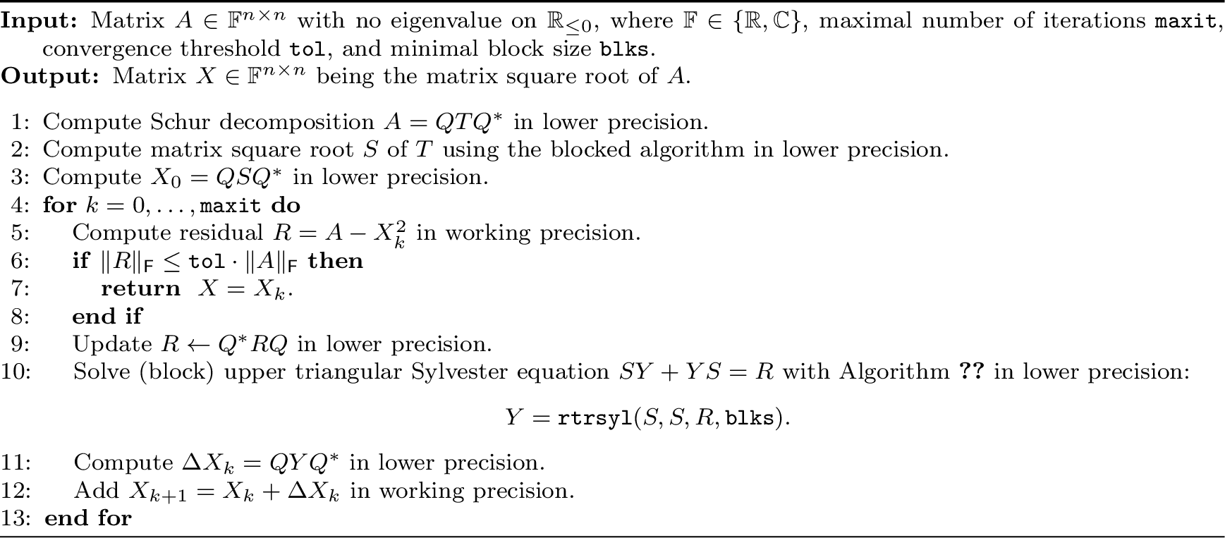
We use the Schur algorithm [1] carried out in lower precision to compute \(X_{0}\). As discussed in Section 1, it starts with computing a Schur decomposition \(A=QTQ^{*}\), where \(T\) is upper triangular and \(Q\) is unitary. The square root \(T^{1/2}\) is then also upper triangular and is computed using the blocked method described in Section 2.2.1 below. Finally, \(X_{0}\) is obtained from the matrix product \(X_{0}=QT^{1/2}Q^{*}\).
A common technique in the Newton method is to freeze the Jacobian throughout the iteration. In the context of our framework above, it means that we freeze \(\hat{X}=X_{0}\) in the correction equation 2 used in Step 3 of our framework as \[X_{0}\cdot\Delta X_{k}+\Delta X_{k}\cdot X_{0}=R_{k}.\] Reusing the Schur decomposition \(X_{0}=QT^{1/2}Q^{*}\) allows us to rewrite this equation as \[\label{eq:triangsylv} S\cdot Y+Y\cdot S={R},\tag{3}\] with \(S=T^{1/2}\), \(\Delta X_{k}=QYQ^{*}\), and the updated right-hand side \(R\gets Q^{*}R_{k}Q\). Because \(S\) has all its eigenvalues in the open right-half complex plane, 3 is uniquely solvable. The triangular structure of \(S\) allows one to solve 3 in \(\mathcal{O}(n^{3})\) operations using a back-substitution procedure. In Section 2.2.2, we will discuss how this can be carried out efficiently with a blocked algorithm.
2.2 Blocked algorithms↩︎
To enhance the performance of our algorithm, we use blocked algorithms to compute the square root of a triangular matrix and solve upper triangular Sylvester equations of the form 3 .
2.2.1 Blocked algorithm for computing square roots of upper triangular matrices↩︎
The standard method for computing the matrix square root \(S=T^{1/2}\) of an upper triangular matrix \(T\) is the following back-substitution technique [1]:
Compute the diagonal entries \(s_{i,i}=t_{i,i}^{1/2}\) for \(i=1,\dotsc,n\);
Compute the other nonzero entries by column. For \(j=2:n\), \(i=j-1:-1:1\), update \[\label{eq:subst} s_{i,j}=\frac{t_{i,j}-\sum_{k=i+1}^{j-1}s_{i,k}s_{k,j}}{s_{i,i}+s_{j,j}}.\tag{4}\]
In [24], Deadman, Higham, and Ralha proposed different blocked algorithms for this procedure. In particular, the block method partitions \(T\) in blocks of roughly equal size. It then carries out the back-substitution technique above on these blocks. For the diagonal blocks, square roots of (small) upper triangular matrices are computed using the technique above. The off-diagonal blocks are computed in (block) column order, solving (small) Sylvester equations instead of 4 . Additionally, [24] proposed a block recursion method, which recursively partitions \(T\) into two-by-two block matrices, but our preliminary numerical experiments reveal little to no performance advantage in our computational setting.
When matrix \(A\) is real, a real Schur decomposition \(A=QTQ^{\top}\) is used, where \(Q\) becomes a real orthogonal matrix and \(T\) is quasi-upper triangular, with \(1\times1\) and \(2\times2\) blocks on the diagonal. The real Schur decomposition is cheaper than the complex Schur decomposition, and only minor changes need to be made to the implementation thereafter. In particular, when performing a block partition, no \(2\times2\) blocks are cut. To simplify the description, we will focus on using the complex Schur form in the following sections.
2.2.2 Block recursion for solving triangular Sylvester equations↩︎
To solve the triangular Sylvester equation 3 in step 3 of our framework, we will make use of the block recursion technique by Jonsson and Kågström [25], [26]. Applied to 3 , this technique starts by partitioning the involved matrices as follows (where \(\tilde{S}=S\)): \[\label{eq:partition} S=\begin{bmatrix}S_{1,1} & S_{1,2} \\ 0 & S_{2,2}\end{bmatrix},\quad \tilde{S}=\begin{bmatrix}\tilde{S}_{1,1} & \tilde{S}_{1,2} \\ 0 & \tilde{S}_{2,2}\end{bmatrix},\quad Y=\begin{bmatrix}Y_{1,1} & Y_{1,2} \\ Y_{2,1} & Y_{2,2}\end{bmatrix},\quad R=\begin{bmatrix} R_{1,1} & R_{1,2} \\ R_{2,1} & R_{2,2}\end{bmatrix},\tag{5}\] such that the diagonal blocks are of size roughly \(n/2\). Then \(SY+Y\tilde{S}=R\) becomes \[\begin{align} S_{1,1}Y_{1,1}+Y_{1,1}\tilde{S}_{1,1} & =R_{1,1}-S_{1,2}Y_{2,1},\\ S_{1,1}Y_{1,2}+Y_{1,2}\tilde{S}_{2,2} & =R_{1,2}-S_{1,2}Y_{2,2}-Y_{1,1}\tilde{S}_{1,2},\\ S_{2,2}Y_{2,1}+Y_{2,1}\tilde{S}_{1,1} & =R_{2,1},\\ S_{2,2}Y_{2,2}+Y_{2,2}\tilde{S}_{2,2} & =R_{2,2}-Y_{2,1}\tilde{S}_{1,2}. \end{align}\]
This reduces the original equation to \(4\) smaller triangular Sylvester equations, which are solved recursively until the matrix sizes are sufficiently small, when the standard Bartels–Stewart method is used. The resulting procedure is outlined in Algorithm 1. Numerical experiments [27] show that the block recursion algorithm offers significant speedup compared with applying the standard Bartels–Stewart method to the original Sylvester equation.
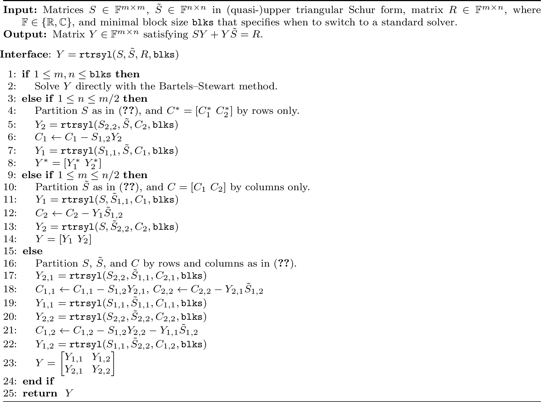
Even though 3 is a particular Sylvester equation with \(\tilde{S}=S\), Algorithm 1 is presented for solving a general triangular Sylvester equation because in lower levels of recursion the Sylvester equations are no longer in that particular form.
2.3 Main algorithms↩︎
Combining the techniques from Sections 2.1 and 2.2 with our framework leads to Algorithm 2, one of the main algorithms proposed in this work.
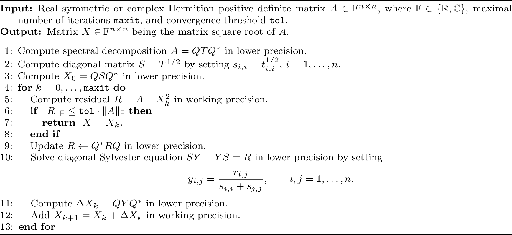
A special case of particular practical importance is the computation of matrix square roots of symmetric, or Hermitian, positive definite matrices. In this setting, the Schur decomposition reduces to the spectral decomposition. Additionally, operations such as computing the square root of a triangular matrix and solving triangular Sylvester equations reduce to computing scalar square roots and solving diagonal Sylvester equations, both of which are straightforward. The resulting simplified procedure is summarized in Algorithm 3.
3 Convergence and accuracy analysis↩︎
In this section, we perform a convergence and accuracy analysis of our mixed precision algorithms for computing matrix square roots. For simplicity, we focus our analysis on real matrices as the analysis for complex matrices is very similar. In Section 3.1, we analyse convergence in exact arithmetic and prove that the iterative refinement converges at least linearly to the matrix square root if the Schur algorithm provides a sufficiently close approximation. In Sections 3.2 and 3.3, we analyse the effect of rounding errors. This turns out to be significantly simpler for the symmetric positive definite case, for which we establish forward stability of Algorithm 3 under some mild conditions. Parts of the analysis carry over to Algorithm 2 for general matrices.
In this section, we use \(\mathop{\mathrm{f{}l}}(\cdot)\) and \(\mathop{\mathrm{f{}l}}_{l}(\cdot)\) to denote computed values in working and lower precision, respectively. Letting \(\boldsymbol{u}\) and \(\boldsymbol{u}_{l}\) denote the corresponding unit roundoffs, we follow the notation from [28] and set \[\label{eq:gamma} \gamma_{n}=\frac{n\boldsymbol{u}}{1-n\boldsymbol{u}},\qquad \gamma_{n}^{l}=\frac{n\boldsymbol{u}_{l}}{1-n\boldsymbol{u}_{l}}.\tag{6}\] Throughout this section, it is tacitly assumed that all these quantities are well defined. For example, when writing \(\gamma_{n}^{l}\), it is assumed that \(n\boldsymbol{u}_{l}<1\).
3.1 Convergence analysis↩︎
To establish convergence of the iterative refinement process in Algorithms 2 and 3 to the matrix square root \(X=A^{1/2}\), we derive relations between the iteration errors in exact arithmetic. It is assumed that the iteration is started by some approximation \(X_{0}\), e.g., the one returned by the Schur algorithm in lower precision. Let \(B_{X_{0}}=I_{n}\otimes X_{0}+X_{0}^{\top}\otimes I_{n}\). Then each iteration in Algorithms 2 and 3 can be compactly written as \[\label{eq:vec} \mathop{\mathrm{vec}}(X_{k+1})=\mathop{\mathrm{vec}}(X_{k})+B_{X_{0}}^{-1}\cdot\mathop{\mathrm{vec}}(A-X_{k}^{2}).\tag{7}\] By the Newton–Kantorovich theorem [29], this iteration converges if \[\lVert B_{X_{0}}^{-1}\rVert_{2}\cdot\bigl\lVert B_{X_{0}}^{-1} \cdot\mathop{\mathrm{vec}}(A-X_{0}^{2})\bigr\rVert_{2}<\frac{1}{4}.\] Letting \(E_{k}=X_{k}-X\) denote the iteration error, this condition can be expressed as \[\label{eq:suff-condition} \lVert B_{X_{0}}^{-1}\rVert_{2}\cdot \bigl\lVert\mathop{\mathrm{vec}}(E_{0})-B_{X_{0}}^{-1}\cdot\mathop{\mathrm{vec}}(E_{0}^{2})\bigr\rVert_{2}<\frac{1}{4}.\tag{8}\] Let \(\mu=2\lVert B_{X_{0}}^{-1}\rVert_{2}\cdot\lVert E_{0}\rVert_{\mathsf F}\). Note that \[4\lVert B_{X_{0}}^{-1}\rVert_{2}\cdot\bigl\lVert\mathop{\mathrm{vec}}(E_{0})-B_{X_{0}}^{-1} \cdot\mathop{\mathrm{vec}}(E_{0}^{2})\bigr\rVert_{2}\leq4\lVert B_{X_{0}}^{-1}\rVert_{2}\lVert E_{0}\rVert_{\mathsf F} +4\lVert B_{X_{0}}^{-1}\rVert_{2}^{2}\lVert E_{0}\rVert_{\mathsf F}^{2}=2\mu+\mu^{2}.\] Therefore if \(\mu<\sqrt{2}-1\), condition 8 holds, and hence iteration 7 converges. In fact, this convergence condition can be further weakened. This is implied by the following theorem, which covers a more general form of \(B\) needed later.
Theorem 1. With the notation introduced above, let \(Z\in\mathbb{R}^{n\times n}\) be such that \(B_{Z}=I_{n}\otimes Z+Z^{\top}\otimes I_{n}\) is invertible and define \(E_{Z}=Z-X\). Then the error \(E_{k}=X_{k}-X\) of the sequence \(\{X_{k}\}\) generated by 7 with such a choice of \(B_{Z}\) satisfies \[\lVert E_{k+1}\rVert_{\mathsf F}\leq 2\lVert B_{Z}^{-1}\rVert_{2}\lVert E_{Z}\rVert_{\mathsf F} \lVert E_{k}\rVert_{\mathsf F}+\lVert B_{Z}^{-1}\rVert_{2}\lVert E_{k}\rVert_{\mathsf F}^{2}.\] Assuming \[\rho_{0}=\lVert B_{Z}^{-1}\rVert_{2}\bigl(2\lVert E_{Z}\rVert_{\mathsf F}+\lVert E_{0}\rVert_{\mathsf F}\bigr)<1,\] it holds that \(\lVert E_{k+1}\rVert_{\mathsf F}\leq\rho_{0}\lVert E_{k}\rVert_{\mathsf F}\), that is, the error converges at least linearly with rate \(\rho_{0}\).
Proof. Note that \[A-X_{k}^{2}=X^{2}-X_{k}^{2} =\frac{1}{2}\bigl[(X+X_{k})(X-X_{k})+(X-X_{k})(X+X_{k})\bigr].\] Define \(e_{k}=-\mathop{\mathrm{vec}}(E_{k})\) as the vectorized iteration error. Then \[\begin{align} e_{k+1} & =\mathop{\mathrm{vec}}(X-X_{k+1})=\mathop{\mathrm{vec}}(X-X_{k})-B_{Z}^{-1}\cdot\mathop{\mathrm{vec}}(A-X_{k}^{2})\\ & =e_{k}-\frac{1}{2}\,B_{Z}^{-1}\cdot\mathop{\mathrm{vec}} \bigl[(X+X_{k})(X-X_{k})+(X-X_{k})(X+X_{k})\bigr]\\ & =e_{k}-\frac{1}{2}\,B_{Z}^{-1}\cdot\bigl[(I_{n}\otimes(X+X_{k})) \mathop{\mathrm{vec}}(X-X_{k})+((X+X_{k})^{\top}\otimes I_{n})\mathop{\mathrm{vec}}(X-X_{k})\bigr]\\ & =\frac{1}{2}\,B_{Z}^{-1}\cdot\bigl[2B_{Z}-I_{n}\otimes(X+X_{k}) -(X+X_{k})^{\top}\otimes I_{n}\bigr]e_{k}\\ & =\frac{1}{2}\,B_{Z}^{-1}\cdot\bigl[I_{n}\otimes(2Z-X-X_{k}) +(2Z-X-X_{k})^{\top}\otimes I_{n}\bigr]e_{k}. \end{align}\] Noting that \(2Z-X-X_{k}=2E_{Z}-E_{k}\), it follows that \[\begin{align} \lVert E_{k+1}\rVert_{\mathsf F} & =\lVert e_{k+1}\rVert_{2} \leq\frac{1}{2}\,\lVert B_{Z}^{-1}\rVert_{2}\cdot\Bigl\lVert\bigl[I_{n}\otimes (2E_{Z}-E_{k})+(2E_{Z}-E_{k})^{\top}\otimes I_{n}\bigr]e_{k}\Bigr\rVert_{2}\\ & =\frac{1}{2}\,\lVert B_{Z}^{-1}\rVert_{2}\cdot\Bigl\lVert \bigl[(2E_{Z}-E_{k})E_{k}+E_{k}(2E_{Z}-E_{k})\bigr]\Bigr\rVert_{\mathsf F}\\ & \leq\lVert B_{Z}^{-1}\rVert_{2}\cdot\lVert E_{k}\rVert_{\mathsf F}\cdot \bigl(\lVert E_{k}\rVert_{\mathsf F}+2\lVert E_{Z}\rVert_{\mathsf F}\bigr). \end{align}\] This shows the first part of the statement. If \(\rho_{0}<1\), it can be shown by induction that \(\lVert E_{k}\rVert_{\mathsf F}\leq\lVert E_{0}\rVert_{\mathsf F}\). This implies the second part of the statement: \(\lVert E_{k+1}\rVert_{\mathsf F}\leq\rho_{0}\lVert E_{k}\rVert_{\mathsf F}\). ◻
3.2 Accuracy analysis for symmetric positive definite matrices↩︎
In this section, we analyse the effect of rounding errors in Algorithm 3 for a symmetric positive definite matrix \(A\). Specifically, we provide a convergence condition and a bound on the limiting accuracy of Algorithm 3 in Theorem 4.
The first step of Algorithm 3 is to compute the spectral decomposition \(A=QTQ^{\top}\). To simplify the analysis, we assume that the standard symmetric QR algorithm is used for this purpose with a constant number of QR iterations per eigenvalue. Then the results from [30] and [28] suggest that the factor \(\hat{Q}\) and the diagonal factor \(\hat{T}\) computed in lower precision satisfy \[\label{eq:assump-Q} A+E=\hat{Q}\hat{T}\hat{Q}^{\top},\tag{9}\] where \(\lVert\hat{Q}^{\top}\hat{Q}-I_{n}\rVert_{2}\leq\gamma_{\mathsf{eig}}(n,\boldsymbol{u}_{l})\), and \(E\) is symmetric with \(\lVert E\rVert_{2}\leq\gamma_{\mathsf{eig}}(n,\boldsymbol{u}_{l})\,\lVert A\rVert_{2}\). Here, \[\label{eq:tgamma} \gamma_{\mathsf{eig}}(n,\boldsymbol{u}_{l})=\frac{cn^{2}\boldsymbol{u}_{l}}{1-cn^{2}\boldsymbol{u}_{l}},\tag{10}\] where \(c\) is a positive constant independent of \(n\), \(\boldsymbol{u}_{l}\), and \(A\). In the following, we tacitly assume that this error bound is well defined, i.e., \(cn^{2}\boldsymbol{u}_{l}<1\) and holds true. We write \(\gamma_{\mathsf{eig}}\equiv\gamma_{\mathsf{eig}}(n,\boldsymbol{u}_{l})\) for simplicity.
The next theorem provides an upper bound for the rounding error effected by the lower precision Schur algorithm, i.e., lines 1–3 of Algorithm 3.
Theorem 2. Recall \(\gamma_{n}^{l}\) from 6 , \(\gamma_{\mathsf{eig}}\) from 10 , and assume that \(\gamma_{\mathsf{eig}}\leq\sqrt{5}-2\). For a symmetric positive definite matrix \(A\), if \(\gamma_{\mathsf{eig}}\cdot\kappa_{2}(A) \leq1/4\), the Schur algorithm in lines 1–3 of Algorithm 3 carried out in lower precision returns a matrix \(\hat{X}_{0}\) that satisfies \[\lVert\hat{X}_{0}-A^{1/2}\rVert_{\mathsf F}\leq2n^{1/2}(1+2n^{1/2}\,\gamma_{2n+1}^{l}) \gamma_{\mathsf{eig}}\cdot\lVert A^{-1}\rVert_{2}^{1/2}\lVert A\rVert_{\mathsf F} +2n^{1/2}\,\gamma_{2n+1}^{l}\cdot\lVert A^{1/2}\rVert_{\mathsf F}.\]
Proof. From \(\lVert\hat{Q}^{\top}\hat{Q}-I_{n}\rVert_{2}\leq\gamma_{\mathsf{eig}}\), we see that \(\lVert\hat{Q}\rVert_{2}^{2}\leq1+\gamma_{\mathsf{eig}}\) and \(\lVert\hat{Q}^{-1}\rVert_{2}^{2}\leq1/(1-\gamma_{\mathsf{eig}})\). Thus \[\label{eq:norm-T} \lVert\hat{T}\rVert_{2}=\lVert\hat{Q}^{-1}(A+E)\hat{Q}^{-\top}\rVert_{2}\leq\lVert\hat{Q}^{-1}\rVert_{2}^{2} \cdot\lVert A+E\rVert_{2}\leq\frac{1}{1-\gamma_{\mathsf{eig}}}\cdot\lVert A+E\rVert_{2}.\tag{11}\]
Note that \(\hat{T}\) is diagonal and positive definite, and, hence, the square root \(\hat{S}=\hat{T}^{1/2}\) is diagonal and positive definite as well, with the diagonal entries computed through \(\hat{s}_{i,i}=\mathop{\mathrm{f{}l}}_{l}\bigl(\hat{t}_{i,i}^{1/2}\bigr)\). By the Wilkinson model [28], there exists a \(\delta_{i}\) such that \[\hat{s}_{i,i}=\hat{t}_{i,i}^{1/2}(1+\delta_{i}),\qquad \lvert\delta_{i}\rvert\leq\boldsymbol{u}_{l},\quad 1\leq i\leq n.\] Hence there exists a diagonal matrix \(H=\mathop{\mathrm{diag}}(\delta_{i})\) such that \[\hat{S}=\hat{T}^{1/2}(I_{n}+H),\qquad\lVert H\rVert_{2}\leq\boldsymbol{u}_{l}.\]
In transforming \(\hat{X}_{0}=\mathop{\mathrm{f{}l}}_{l}(\hat{Q}\hat{S}\hat{Q}^{\top})\), there exists a matrix \(F\) such that \[\hat{X}_{0}=\hat{Q}\hat{S}\hat{Q}^{\top}+F,\] where the componentwise error bound \(\lvert F\rvert\leq \gamma_{2n}^{l}\lvert\hat{Q}\rvert\lvert\hat{S}\rvert\lvert\hat{Q}^{\top}\rvert\) in [28] can be used to imply that \[\lVert F\rVert_{\mathsf F}\leq\gamma_{2n}^{l}(1+\boldsymbol{u}_{l})(1+\gamma_{\mathsf{eig}}) \cdot n^{1/2}\cdot\lVert\hat{T}^{1/2}\rVert_{\mathsf F}.\]
Note that \[\label{eq:X0} \hat{X}_{0}-A^{1/2}=\hat{Q}\hat{S}\hat{Q}^{\top}+F-A^{1/2} =\hat{Q}\hat{T}^{1/2}\hat{Q}^{\top}+\hat{Q}\hat{T}^{1/2}H\hat{Q}^{\top}+F-A^{1/2}.\tag{12}\] Let \(\hat{Q}^{\top}\hat{Q}=I_{n}+J\), with \(\lVert J\rVert_{2}\leq\gamma_{\mathsf{eig}}\). We can now choose \(G\) such that \[\label{eq:error-G} (A+E+G)^{1/2}=\hat{Q}\hat{T}^{1/2}\hat{Q}^{\top},\tag{13}\] where by squaring both sides of 13 , \[G=\hat{Q}\hat{T}^{1/2}(I_{n}+J)\hat{T}^{1/2}\hat{Q}^{\top}-A-E =\hat{Q}\hat{T}^{1/2}J\hat{T}^{1/2}\hat{Q}^{\top}.\] Since \(0\leq\gamma_{\mathsf{eig}}\leq\sqrt{5}-2\), \((1+\gamma_{\mathsf{eig}})^{2}\leq2(1-\gamma_{\mathsf{eig}})\). As \(\lVert E\rVert_{2}\leq\gamma_{\mathsf{eig}}\,\lVert A\rVert_{2}\), we have \[\lVert G\rVert_{2}\leq\lVert\hat{Q}\rVert_{2}^{2}\lVert J\rVert_{2}\lVert\hat{T}\rVert_{2}\leq \frac{\gamma_{\mathsf{eig}}(1+\gamma_{\mathsf{eig}})}{1-\gamma_{\mathsf{eig}}}\lVert A+E\rVert_{2}\leq \frac{\gamma_{\mathsf{eig}}(1+\gamma_{\mathsf{eig}})^{2}}{1-\gamma_{\mathsf{eig}}}\lVert A\rVert_{2}\leq2\gamma_{\mathsf{eig}}\,\lVert A\rVert_{2}.\] Then \(\lVert E+G\rVert_{2}\leq3\gamma_{\mathsf{eig}}\,\lVert A\rVert_{2}\), and \(\lVert E+G\rVert_{\mathsf F}\leq n^{1/2} \lVert E+G\rVert_{2}\leq3n^{1/2}\gamma_{\mathsf{eig}}\,\lVert A\rVert_{2}\leq3n^{1/2}\gamma_{\mathsf{eig}}\,\lVert A\rVert_{\mathsf F}\). It follows from \(\lVert E+G\rVert_{2}\leq3\gamma_{\mathsf{eig}}\,\lVert A\rVert_{2}\leq3/4\cdot\lVert A^{-1}\rVert_{2} ^{-1}=3/4\cdot\lambda_{\min}(A)\) that \(A+E+G\) is symmetric positive definite. Then by [1], \[\begin{align} \lVert(A+E+G)^{1/2}-A^{1/2}\rVert_{\mathsf F} & \leq\frac{\lVert E+G\rVert_{\mathsf F}}{\lambda_{\min}^{1/2}(A)+\lambda_{\min}^{1/2}(A+E+G)}\\ & \leq\frac{\lVert E+G\rVert_{\mathsf F}}{\lambda_{\min}^{1/2}(A)+(\lambda_{\min}(A) -\lVert E+G\rVert_{2})^{1/2}}\leq2n^{1/2}\gamma_{\mathsf{eig}}\cdot\lVert A^{-1}\rVert_{2}^{1/2}\lVert A\rVert_{\mathsf F}. \end{align}\]
Similarly to 11 , since \(\hat{T}^{1/2}=\hat{Q}^{-1} (A+E+G)^{1/2}\hat{Q}^{-\top}\), we see that \(\lVert\hat{T}^{1/2}\rVert_{\mathsf F} \leq\lVert(A+E+G)^{1/2}\rVert_{\mathsf F}/(1-\gamma_{\mathsf{eig}})\). This leads to \[\lVert\hat{Q}\hat{T}^{1/2}H\hat{Q}^{\top}\rVert_{\mathsf F}\leq\frac{\boldsymbol{u}_{l}(1+\gamma_{\mathsf{eig}})}{1-\gamma_{\mathsf{eig}}}\lVert(A+E+G)^{1/2}\rVert_{\mathsf F}\] and \[\lVert F\rVert_{\mathsf F}\leq\frac{\gamma_{2n}^{l}(1+\boldsymbol{u}_{l})(1+\gamma_{\mathsf{eig}})}{1-\gamma_{\mathsf{eig}}}\cdot n^{1/2}\cdot\lVert(A+E+G)^{1/2}\rVert_{\mathsf F}.\] Therefore from 12 , as \(1+\gamma_{\mathsf{eig}}\leq2(1-\gamma_{\mathsf{eig}})\), \[\begin{align} \lVert\hat{X}_{0}-A^{1/2}\rVert_{\mathsf F} & \leq\lVert(A+E+G)^{1/2}-A^{1/2}\rVert_{\mathsf F} +\lVert\hat{Q}\hat{T}^{1/2}H\hat{Q}^{\top}\rVert_{\mathsf F}+\lVert F\rVert_{\mathsf F}\\ & \leq\lVert(A+E+G)^{1/2}-A^{1/2}\rVert_{\mathsf F}+n^{1/2}\,\gamma_{2n+1}^{l}\cdot \frac{1+\gamma_{\mathsf{eig}}}{1-\gamma_{\mathsf{eig}}}\cdot\lVert(A+E+G)^{1/2}\rVert_{\mathsf F}\\ & \leq(1+2n^{1/2}\,\gamma_{2n+1}^{l})\cdot\lVert(A+E+G)^{1/2} -A^{1/2}\rVert_{\mathsf F}+2n^{1/2}\,\gamma_{2n+1}^{l}\cdot\lVert A^{1/2}\rVert_{\mathsf F}\\ & \leq2n^{1/2}(1+2n^{1/2}\,\gamma_{2n+1}^{l})\gamma_{\mathsf{eig}}\cdot\lVert A^{-1}\rVert_{2} ^{1/2}\lVert A\rVert_{\mathsf F}+2n^{1/2}\,\gamma_{2n+1}^{l}\cdot\lVert A^{1/2}\rVert_{\mathsf F}. \end{align}\] ◻
We then consider the iterative refinement process in lines 4–13 of Algorithm 3. Define \(\tilde{X}_{0}=\hat{Q}\hat{S}\hat{Q}^{\top}\), where the factor \(\hat{Q}\) and diagonal factor \(\hat{S}\) from Theorem 2 are the ones returned by the Schur algorithm in lower precision and are later used in iterative refinement.
In Theorem 3, we shall derive the relation between the errors \(\{E_{k}\}\) in each iterative refinement step, combining both the iteration errors bounded by Theorem 1 and additional rounding errors during iterative refinement.
Theorem 3. Recall \(\gamma_{n}, \gamma_{n}^{l}\) from 6 and \(\gamma_{\mathsf{eig}}\) from 10 , and assume that \(\gamma_{\mathsf{eig}}\leq\sqrt{5}-2\). Consider a symmetric positive definite matrix \(A\) with \(\gamma_{\mathsf{eig}}\cdot \kappa_{2}(A)<1\), and recall that \(\hat{X}_{0}\) and \(\{\hat{X}_{k}\}\) are the matrices produced by the Schur algorithm and iterative refinement in Algorithm 3, respectively, carried out in lower/working precision. Recall \(X=A^{1/2}\) and \(\tilde{X}_{0}\) defined before, and let \(B_{\tilde{X}_{0}}=I_{n}\otimes\tilde{X}_{0} +\tilde{X}_{0}^{\top}\otimes I_{n}\). Then the errors \(E_{k}=\hat{X}_{k}-X\) satisfy the recursion \[\lVert E_{k+1}\rVert_{\mathsf F}\leq\nu\lVert E_{k}\rVert_{\mathsf F}+\beta\lVert E_{k}\rVert_{\mathsf F}^{2}+\xi_{k},\] where \[\nu=2\bigl\lVert B_{\tilde{X}_{0}}^{-1}\bigr\rVert_{2} \bigl(\lVert\tilde{X}_{0}-X\rVert_{\mathsf F}+2\epsilon_{l}\lVert X\rVert_{\mathsf F}\bigr), \qquad\beta=(1+2\epsilon_{l})\,\bigl\lVert B_{\tilde{X}_{0}}^{-1}\bigr\rVert_{2},\] with \(\epsilon_{l}=\gamma_{n^{1/2}(4n+3)}^{l} +4\gamma_{\mathsf{eig}}\cdot\kappa_{2}(B_{\tilde{X}_{0}})\), and \[\xi_{k}=2\gamma_{n+1}(1+\epsilon_{l})\,\bigl\lVert B_{\tilde{X}_{0}}^{-1}\bigr\rVert_{2}\cdot (\lVert A\rVert_{\mathsf F}+\lVert\hat{X}_{k}\rVert_{\mathsf F}^{2})+\gamma_{1}\lVert\hat{X}_{k+1}\rVert_{\mathsf F}.\]
Proof. The first step in each iterative refinement loop is to compute the residual in working precision. Let \(R_{k}=A-\hat{X}_{k}^{2}\). Suppose \(\hat{P}_{k}=\mathop{\mathrm{f{}l}}(R_{k})=\mathop{\mathrm{f{}l}}(A-\hat{X}_{k}^{2})\). Then there exists a \(\Delta P_{k}\) such that \[\hat{P}_{k}=R_{k}+\Delta P_{k},\qquad \lVert\Delta P_{k}\rVert_{\mathsf F}\leq\gamma_{n+1}(\lVert A\rVert_{\mathsf F}+\lVert\hat{X}_{k}\rVert_{\mathsf F}^{2}).\] The error bound can be derived from the matrix multiplication error bounds in [28]. This is then followed by converting \(\hat{P}_{k}\) to lower precision: \(\hat{R}_{k}=\mathop{\mathrm{f{}l}}_{l}(\hat{P}_{k})=\hat{P}_{k}+\Delta F_{k}\), with \(\lVert\Delta F_{k}\rVert_{\mathsf F}\leq\boldsymbol{u}_{l}\,\lVert\hat{P}_{k}\rVert_{\mathsf F}\). Setting \(\Delta R_{k}=\Delta P_{k}+\Delta F_{k}\), we obtain \[\hat{R}_{k}=R_{k}+\Delta P_{k}+\Delta F_{k}=R_{k}+\Delta R_{k},\] where \[\lVert\Delta R_{k}\rVert_{\mathsf F}\leq\lVert\Delta P_{k}\rVert_{\mathsf F} +\lVert\Delta F_{k}\rVert_{\mathsf F}\leq\boldsymbol{u}_{l}\lVert R_{k}\rVert_{\mathsf F} +(1+\boldsymbol{u}_{l})\gamma_{n+1}(\lVert A\rVert_{\mathsf F}+\lVert\hat{X}_{k}\rVert_{\mathsf F}^{2}).\] Therefore \[\lVert\hat{R}_{k}\rVert_{\mathsf F}\leq\lVert R_{k}\rVert_{\mathsf F} +\lVert\Delta R_{k}\rVert_{\mathsf F}\leq(1+\boldsymbol{u}_{l})\,\lVert R_{k}\rVert_{\mathsf F} +(1+\boldsymbol{u}_{l})\gamma_{n+1}(\lVert A\rVert_{\mathsf F}+\lVert\hat{X}_{k}\rVert_{\mathsf F}^{2}).\]
The next step consists of solving a (diagonal) Sylvester equation. When forming the right-hand side \(\hat{Q}^{\top}\hat{R}_{k}\hat{Q}\), similarly to the proof of Theorem 2, the componentwise error bound in [28] can be used to imply that there exists a \(\delta R_{k}\) that satisfies \[\mathop{\mathrm{f{}l}}_{l}(\hat{Q}^{\top}\hat{R}_{k}\hat{Q}) =\hat{Q}^{\top}\hat{R}_{k}\hat{Q}+\delta R_{k},\qquad\lVert\delta R_{k}\rVert_{\mathsf F} \leq n^{1/2}\,\gamma_{2n}^{l}\cdot\lVert\hat{Q}\rVert_{2}^{2}\lVert\hat{R}_{k}\rVert_{\mathsf F}.\]
Note that the assumption \(\gamma_{\mathsf{eig}}\cdot\kappa_{2}(A)<1\) implies that the computed diagonal square root \(\hat{S}\) is positive definite and, hence, \(B_{\hat{S}}=I_{n}\otimes\hat{S}+\hat{S}\otimes I_{n}\) is invertible. Suppose that \(\bar{Y}_{k}\) is the exact solution to \(\hat{S}Y_{k} +Y_{k}\hat{S}=\hat{Q}^{\top}\hat{R}_{k}\hat{Q}\), and that \(\hat{Y}_{k}\) is the computed solution (in lower precision) to \(\hat{S}Y_{k}+Y_{k}\hat{S} =\mathop{\mathrm{f{}l}}_{l}(\hat{Q}^{\top}\hat{R}_{k}\hat{Q})\), respectively. By [28] and the Wilkinson model, as there are two floating-point operations for computing each element, \[\begin{align} \lVert\hat{Y_{k}}-\bar{Y}_{k}\rVert_{\mathsf F} & \leq\lVert B_{\hat{S}}^{-1}\rVert_{2}\cdot\bigl(\gamma^l_{2}\,\lVert\hat{Q} ^{\top}\hat{R}_{k}\hat{Q}+\delta R_{k}\rVert_{\mathsf F}+\lVert\delta R_{k}\rVert_{\mathsf F}\bigr)\\ & \leq n^{1/2}\,(\gamma_{2}^{l}(1+\gamma_{2n}^{l})+\gamma_{2n}^{l}) \cdot\lVert B_{\hat{S}}^{-1}\rVert_{2}\lVert\hat{Q}\rVert_{2}^{2}\lVert\hat{R}_{k}\rVert_{\mathsf F}\\ & \leq n^{1/2}\,\gamma_{2n+2}^{l}\cdot\lVert B_{\hat{S}}^{-1}\rVert_{2} \lVert\hat{Q}\rVert_{2}^{2}\lVert\hat{R}_{k}\rVert_{\mathsf F}. \end{align}\]
Similarly in forming \(\hat{Q}\hat{Y}\hat{Q}^{\top}\), by [28], there exists a \(\Delta Y_{k}\) such that \[\Delta\hat{X}_{k}=\mathop{\mathrm{f{}l}}_{l}(\hat{Q}\hat{Y}_{k}\hat{Q}^{\top}) =\hat{Q}\hat{Y}_{k}\hat{Q}^{\top}+\Delta Y_{k},\qquad\lVert\Delta Y_{k}\rVert_{\mathsf F} \leq n^{1/2}\,\gamma_{2n}^{l}\cdot\lVert\hat{Q}\rVert_{2}^{2}\lVert\hat{Y}_{k}\rVert_{\mathsf F}.\] Denote \(\Delta\bar{X}_{k}=\hat{Q}\bar{Y}_{k}\hat{Q}^{\top}\). Noting \(\lVert\bar{Y}_{k}\rVert_{\mathsf F}\leq\lVert B_{\hat{S}}^{-1}\rVert_{2} \lVert\hat{Q}\rVert_{2}^{2}\lVert\hat{R}_{k}\rVert_{\mathsf F}\), we have \[\begin{align} \lVert\Delta\hat{X}_{k}-\Delta\bar{X}_{k}\rVert_{\mathsf F} & \leq\lVert\hat{Q}\hat{Y}_{k} \hat{Q}^{\top}-\hat{Q}\bar{Y}_{k}\hat{Q}^{\top}\rVert_{\mathsf F}+\lVert\Delta Y_{k}\rVert_{\mathsf F}\notag\\ & \leq(1+\gamma_{\mathsf{eig}})\,\lVert\hat{Y_{k}}-\bar{Y}_{k}\rVert_{\mathsf F} +n^{1/2}\,\gamma_{2n}^{l}(1+\gamma_{\mathsf{eig}})\cdot \bigl(\lVert\hat{Y_{k}}-\bar{Y}_{k}\rVert_{\mathsf F}+\lVert\bar{Y}_{k}\rVert_{\mathsf F}\bigr)\notag\\ & \leq(1+n^{1/2}\,\gamma_{2n}^{l})(1+\gamma_{\mathsf{eig}})\cdot \lVert\hat{Y_{k}}-\bar{Y}_{k}\rVert_{\mathsf F}+n^{1/2}\,\gamma_{2n}^{l} (1+\gamma_{\mathsf{eig}})\cdot\lVert\bar{Y}_{k}\rVert_{\mathsf F}\notag\\ & \leq\gamma_{n^{1/2}(4n+2)}^{l}\,(1+\gamma_{\mathsf{eig}})^{2}\cdot \lVert B_{\hat{S}}^{-1}\rVert_{2}\lVert\hat{R}_{k}\rVert_{\mathsf F}\label{eq:bound-spd-1}. \end{align}\tag{14}\]
Suppose \(\Delta\check{X}_{k}\) is the exact solution to \(\tilde{X}_{0}\Delta X_{k}+\Delta X_{k}\tilde{X}_{0}=\hat{R}_{k}\). Define \(\mathcal{L}(X)=\tilde{X}_0X+X\tilde{X}_0\). Then \(\Delta\check{X}_{k}=\mathcal{L}^{-1}(\hat{R}_{k})\). Let \(\hat{Q}^{\top}\hat{Q}=I+J\), \(\hat{Q}\hat{Q}^{\top}=I+K\), with \(\lVert J\rVert_{2}=\lVert K\rVert_{2}\leq\gamma_{\mathsf{eig}}\). Then \[\begin{align} \mathcal{L}(\Delta\bar{X}_{k}) & = \hat{Q}\hat{S}\hat{Q}^{\top}\hat{Q}\bar{Y}_{k}\hat{Q}^{\top} +\hat{Q}\bar{Y}_{k}\hat{Q}^{\top}\hat{Q}\hat{S}\hat{Q}^{\top}\\ & =\hat{Q}(\hat{S}\bar{Y}_{k}+\bar{Y}_{k}\hat{S})\hat{Q}^{\top} +\hat{Q}(\hat{S}J\bar{Y}_{k}+\bar{Y}_{k}J\hat{S})\hat{Q}^{\top}\\ & =\hat{Q}\hat{Q}^{\top}\hat{R}_{k}\hat{Q}\hat{Q}^{\top} +\hat{Q}(\hat{S}J\bar{Y}_{k}+\bar{Y}_{k}J\hat{S})\hat{Q}^{\top}\\ & =\hat{R}_{k}+K\hat{R}_{k}+\hat{R}_{k}K+K\hat{R}_{k}K +\hat{Q}(\hat{S}J\bar{Y}_{k}+\bar{Y}_{k}J\hat{S})\hat{Q}^{\top}. \end{align}\] Recall that \(\lVert\bar{Y}_{k}\rVert_{\mathsf F}\leq\lVert B_{\hat{S}}^{-1}\rVert_{2} \lVert\hat{Q}\rVert_{2}^{2}\lVert\hat{R}_{k}\rVert_{\mathsf F}\). Hence \[\begin{align} \lVert\mathcal{L}(\Delta\bar{X}_{k})-\hat{R}_{k}\rVert_{\mathsf F} & \leq(2\lVert K\rVert_{2}+\lVert K\rVert_{2}^{2})\,\lVert\hat{R}_{k}\rVert_{\mathsf F} +2\lVert\hat{Q}\rVert_{2}^{2}\lVert\hat{S}\rVert_{2}\lVert J\rVert_{2}\lVert\bar{Y}_{k}\rVert_{\mathsf F}\\ & \leq\bigl(2\gamma_{\mathsf{eig}}+\gamma_{\mathsf{eig}}^{2}+2\gamma_{\mathsf{eig}}(1+\gamma_{\mathsf{eig}})^{2}\, \lVert B_{\hat{S}}^{-1}\rVert_{2}\lVert\hat{S}\rVert_{2}\bigr)\cdot\lVert\hat{R}_{k}\rVert_{\mathsf F}. \end{align}\]
Note that \(\tilde{X}_{0}=\hat{Q}\hat{S}\hat{Q}^{\top}\) is similar to \(\hat{S}^{1/2}\hat{Q}^{\top}\hat{Q}\hat{S}^{1/2}\). Hence \[\lambda_{\min}(\tilde{X}_{0})=\lambda_{\min}(\hat{S}^{1/2}\hat{Q} ^{\top}\hat{Q}\hat{S}^{1/2})\leq(1+\gamma_{\mathsf{eig}})\,\lambda_{\min}(\hat{S}).\] As \(B_{\tilde{X}_{0}}=I_{n}\otimes\tilde{X}_{0} +\tilde{X}_{0}^{\top}\otimes I_{n}\), it follows that \[\lVert B_{\hat{S}}^{-1}\rVert_{2}=\frac{1}{\lambda_{\min}(B_{\hat{S}})} =\frac{1}{2\lambda_{\min}(\hat{S})}\leq\frac{1+\gamma_{\mathsf{eig}}}{2\lambda_{\min} (\tilde{X}_{0})}=\frac{1+\gamma_{\mathsf{eig}}}{\lambda_{\min}(B_{\tilde{X}_{0}})} =(1+\gamma_{\mathsf{eig}})\lVert B_{\tilde{X}_{0}}^{-1}\rVert_{2}.\] Hence similarly to 11 , \[1\leq\kappa_{2}(\hat{S})=2\lVert B_{\hat{S}}^{-1}\rVert_{2}\lVert\hat{S}\rVert_{2} \leq2(1+\gamma_{\mathsf{eig}}) \lVert B_{\tilde{X}_{0}}^{-1}\rVert_{2}\cdot\frac{\lVert\tilde{X}_{0}\rVert_{2}}{1-\gamma_{\mathsf{eig}}} \leq\frac{1+\gamma_{\mathsf{eig}}}{1-\gamma_{\mathsf{eig}}}\cdot\kappa_{2}(B_{\tilde{X}_{0}}).\]
As \(\Delta\check{X}_{k}-\Delta\bar{X}_{k}=\mathcal{L}^{-1} \bigl(\hat{R}_{k}-\mathcal{L}(\Delta\bar{X}_{k})\bigr)\), and \(3\gamma_{\mathsf{eig}}+\gamma_{\mathsf{eig}}^{2}<1\), by [28], \[\begin{align} \lVert\Delta\check{X}_{k}-\Delta\bar{X}_{k}\rVert_{\mathsf F} & \leq\lVert B_{\tilde{X}_{0}} ^{-1}\rVert_{2}\cdot\lVert\mathcal{L}(\Delta\bar{X}_{k})-\hat{R}_{k}\rVert_{\mathsf F}\notag\\ & \leq\bigl(2\gamma_{\mathsf{eig}}+\gamma_{\mathsf{eig}}^{2}+\gamma_{\mathsf{eig}}(1+\gamma_{\mathsf{eig}})^{2}\,\kappa_{2} (\hat{S})\bigr)\cdot\lVert B_{\tilde{X}_{0}}^{-1}\rVert_{2}\lVert\hat{R}_{k}\rVert_{\mathsf F}\notag\\ & \leq(3\gamma_{\mathsf{eig}}+3\gamma_{\mathsf{eig}}^{2}+\gamma_{\mathsf{eig}}^{3})\cdot\kappa_{2}(\hat{S}) \cdot\lVert B_{\tilde{X}_{0}}^{-1}\rVert_{2}\lVert\hat{R}_{k}\rVert_{\mathsf F}\notag\\ & \leq\frac{4\gamma_{\mathsf{eig}}(1+\gamma_{\mathsf{eig}})}{1-\gamma_{\mathsf{eig}}}\cdot\kappa_{2} (B_{\tilde{X}_{0}})\cdot\lVert B_{\tilde{X}_{0}}^{-1}\rVert_{2}\lVert\hat{R}_{k}\rVert_{\mathsf F} \label{eq:bound-spd-2} \end{align}\tag{15}\]
Suppose \(\Delta\tilde{X}_{k}\) is the exact solution to \(\tilde{X}_{0}\Delta X_{k}+\Delta X_{k}\tilde{X}_{0}=R_{k}\). Then \[\label{eq:bound-spd-3} \lVert\Delta\tilde{X}_{k}-\Delta\check{X}_{k}\rVert_{\mathsf F}\leq \lVert B_{\tilde{X}_{0}}^{-1}\rVert_{2}\cdot\lVert R_{k}-\hat{R}_{k}\rVert_{\mathsf F} =\lVert B_{\tilde{X}_{0}}^{-1}\rVert_{2}\lVert\Delta R_{k}\rVert_{\mathsf F}.\tag{16}\]
The final updating step in working precision can be expressed as \[\hat{X}_{k+1}=\mathop{\mathrm{f{}l}}(\hat{X}_{k}+\Delta\hat{X}_{k}) =\hat{X}_{k}+\Delta\hat{X}_{k}+\delta\hat{X}_{k},\qquad \lVert\delta\hat{X}_{k}\rVert_{\mathsf F}\leq\gamma_{1}\lVert\hat{X}_{k+1}\rVert_{\mathsf F}.\] This is equivalent to \[\hat{X}_{k+1}=\hat{X}_{k}+\Delta\tilde{X}_{k}+(\Delta\check{X}_{k} -\Delta\tilde{X}_{k})+(\Delta\bar{X}_{k}-\Delta\check{X}_{k}) +(\Delta\hat{X}_{k}-\Delta\bar{X}_{k})+\delta\hat{X}_{k}.\]
As \(\gamma_{\mathsf{eig}}\leq(1+\gamma_{\mathsf{eig}})(1-\gamma_{\mathsf{eig}})\), the rounding error \(G_{k}=\hat{X}_{k+1}-\hat{X}_{k}-\Delta\tilde{X}_{k}\), by 14 , 15 , and 16 , satisfies \[\begin{align} \lVert G_{k}\rVert_{\mathsf F} & \leq\lVert\Delta\tilde{X}_{k}-\Delta\check{X}_{k}\rVert_{\mathsf F} +\lVert\Delta\bar{X}_{k}-\Delta\check{X}_{k}\rVert_{\mathsf F} +\lVert\Delta\hat{X}_{k}-\Delta\bar{X}_{k}\rVert_{\mathsf F}+\lVert\delta\hat{X}_{k}\rVert_{\mathsf F}\\ & \leq\lVert B_{\tilde{X}_{0}}^{-1}\rVert_{2}\,\bigl(\lVert\Delta R_{k}\rVert_{\mathsf F} +\bigl(\gamma_{n^{1/2}(4n+2)}^{l}(1+\gamma_{\mathsf{eig}})^{3}+\frac{4\gamma_{\mathsf{eig}} (1+\gamma_{\mathsf{eig}})}{1-\gamma_{\mathsf{eig}}}\kappa_{2}(B_{\tilde{X}_{0}})\bigr) \lVert\hat{R}_{k}\rVert_{\mathsf F}\bigr)+\gamma_{1}\lVert\hat{X}_{k+1}\rVert_{\mathsf F}\\ & \leq\frac{(1+\gamma_{\mathsf{eig}})^{2}}{1-\gamma_{\mathsf{eig}}}\cdot\lVert B_{\tilde{X}_{0}}^{-1}\rVert_{2} \cdot\bigl(\epsilon_{l}\,\lVert R_{k}\rVert_{\mathsf F}+\gamma_{n+1}(1+\epsilon_{l}) (\lVert A\rVert_{\mathsf F}+\lVert\hat{X}_{k}\rVert_{\mathsf F}^{2})\bigr)+\gamma_{1}\lVert\hat{X}_{k+1}\rVert_{\mathsf F}. \end{align}\]
Note that \[\lVert R_{k}\rVert_{\mathsf F}=\lVert\hat{X}_{k}^{2}-X^{2}\rVert_{\mathsf F}=\lVert XE_{k} +E_{k}\hat{X}_{k}\rVert_{\mathsf F}\leq(\lVert X\rVert_{\mathsf F}+\lVert\hat{X}_{k}\rVert_{\mathsf F})\lVert E_{k}\rVert_{\mathsf F} \leq2\lVert X\rVert_{\mathsf F}\lVert E_{k}\rVert_{\mathsf F}+\lVert E_{k}\rVert_{\mathsf F}^{2}.\] As \(0\leq\gamma_{\mathsf{eig}}\leq\sqrt{5}-2\), \((1+\gamma_{\mathsf{eig}})^{2}\leq2(1-\gamma_{\mathsf{eig}})\). Therefore, \[\label{eq:G} \lVert G_{k}\rVert_{\mathsf F}\leq4\epsilon_{l}\,\lVert B_{\tilde{X}_{0}}^{-1}\rVert_{2} \lVert X\rVert_{\mathsf F}\lVert E_{k}\rVert_{\mathsf F} +2\epsilon_{l}\,\lVert B_{\tilde{X}_{0}}^{-1}\rVert_{2}\lVert E_{k}\rVert_{\mathsf F}^{2}+\xi_{k}.\tag{17}\]
Recall that \(\hat{X}_{k+1}=(\hat{X}_{k}+\Delta\tilde{X}_{k})+G_{k}\). Applying Theorem 1 with \(Z=\tilde{X}_{0}\) gives \[\lVert(\hat{X}_{k}+\Delta\tilde{X}_{k})-X\rVert_{\mathsf F}\leq 2\lVert B_{\tilde{X}_{0}}^{-1}\rVert_{2}\cdot\lVert\tilde{X}_{0}-X\rVert_{\mathsf F}\cdot \lVert E_{k}\rVert_{\mathsf F}+\lVert B_{\tilde{X}_{0}}^{-1}\rVert_{2}\cdot\lVert E_{k}\rVert_{\mathsf F}^{2}.\] Combining this with 17 , we obtain \[\begin{align} \lVert E_{k+1}\rVert_{\mathsf F} & \leq 2\lVert B_{\tilde{X}_{0}}^{-1}\rVert_{2}\cdot\lVert\tilde{X}_{0}-X\rVert_{\mathsf F}\cdot\lVert E_{k}\rVert_{\mathsf F} +\lVert B_{\tilde{X}_{0}}^{-1}\rVert_{2}\cdot\lVert E_{k}\rVert_{\mathsf F}^{2}+\lVert G_{k}\rVert_{\mathsf F}\\ & \leq2\lVert B_{\tilde{X}_{0}}^{-1}\rVert_{2}\cdot\bigl(\lVert\tilde{X}_{0}-X\rVert_{\mathsf F} +2\epsilon_{l}\lVert X\rVert_{\mathsf F}\bigr)\cdot\lVert E_{k}\rVert_{\mathsf F}+(1+2\epsilon_{l})\, \lVert B_{\tilde{X}_{0}}^{-1}\rVert_{2}\cdot\lVert E_{k}\rVert_{\mathsf F}^{2}+\xi_{k}. \end{align}\] This proves the claimed recursion. ◻
The framework of the proof is similar to those of previous works, where we sequentially analyse the computational procedures and then use the triangle inequality to derive a forward error relation. The complexity of the proof is due to the fact that we do not assume the orthogonality of \(\hat{Q}\) but instead utilize a parameter \(\gamma_{\mathsf{eig}}\), which is more rigorous. The analysis in Theorems 2 and 3 relies on \(\gamma_{\mathsf{eig}}<1\). The stronger requirement \(\gamma_{\mathsf{eig}}\leq\sqrt{5}-2\) is made primarily to simplify the analysis. For a slightly larger \(\gamma_{\mathsf{eig}}\), there is still a similar result, though certain constants will be larger.
In Theorem 3, we utilize \(\hat{X}_{0}\) and \(\tilde{X}_{0}=\hat{Q}\hat{S}\hat{Q}^{\top}\) in coherence with the procedures in Algorithm 3. Specifically, \(\hat{X}_{0}\) is employed as the first iterate of the computed matrices \(\{\hat{X}_{k}\}\), and factors \(\hat{Q}\) and \(\hat{S}\) (which collectively form \(\tilde{X}_{0}\)) are used to solve the correction equation. Both \(\hat{X}_{0}\) and \(\tilde{X}_{0}\) can be seen as different approximations of \(X_{0}\) in finite arithmetic.
To turn the recursive inequality of Theorem 3 into an explicit bound, we will make use of the following lemma.
Lemma 1. Consider the nonnegative scalar sequence \(\{x_{k}\}\): \(x_{k+1}=\alpha x_{k} +\theta x_{k}^{2}+\zeta\), where \(\alpha\), \(\theta\), \(\zeta>0\), \(\alpha<1\), and the discriminant \(\Delta=(1-\alpha)^{2}-4\theta\zeta>0\). Let \(0<x_{L}<x_{R}\) be the solutions to \[x=\alpha x+\theta x^{2}+\zeta.\] If \(0\leq x_{0}<x_{R}\), the sequence \(\{x_{k}\}\) converges to \(x_{L}\) at least linearly with \[\lvert x_{k}-x_{L}\rvert\leq\rho^{k}\lvert x_{0}-x_{L}\rvert,\] where \(\rho=\max\bigl(\theta(x_{0}+x_{L})+\alpha, 1-\sqrt{\Delta}\,\bigr)<1\).
Proof. Let \(\delta_{k}=x_{k}-x_{L}\). Then \[\delta_{k+1}=x_{k+1}-x_{L}=\alpha(x_{k}-x_{L})+\theta(x_{k}^{2}-x_{L}^{2}) =(\alpha+\theta(x_{k}+x_{L}))\,\delta_{k}.\] By induction it is easy to show that \(x_{k}<x_{R}\) for all \(k\geq0\). Let \(\lambda_{k}=\alpha+\theta(x_{k}+x_{L})>0\), where \[\lambda_{k}<\alpha+\theta(x_{R}+x_{L}) =\alpha+\theta\cdot\frac{1-\alpha}{\theta}=1.\] Define \(\rho:=\sup\nolimits_{j\geq 0}\lambda_{j}\). Then \(\rho\leq 1\). Using \(\lvert\delta_{k+1}\rvert=\lambda_{k}\lvert\delta_{k}\rvert\), we have \(\lvert\delta_{k}\rvert\leq\rho^{k}\lvert\delta_{0}\rvert\).
1.3
If \(x_{L}\leq x_{0}<x_{R}\), \(\{x_{k}\}\) is decreasing. In this case \(\rho=\alpha+\theta(x_{0}+x_{L})\).
If \(0\leq x_{0}<x_{L}\), \(\{x_{k}\}\) is increasing. In this case \(\rho=\alpha+2\theta x_{L}=1-\sqrt{(1-\alpha)^{2}-4\theta\zeta}\).
Either case, \(\rho=\max\bigl(\theta(x_{0}+x_{L})+\alpha, 1-\sqrt{(1-\alpha)^{2}-4\theta\zeta}\,\bigr)<1\) as claimed. ◻
From Lemma 1, we see that if \(0\leq x_{0}\leq(1-\alpha)/2\theta<x_{R}\), for \(k\geq0\), \[\begin{align} x_{k} \leq x_{L}+\rho^{k}\lvert x_{0}-x_{L}\rvert & =\frac{1-\alpha-\sqrt{\Delta}}{2\theta}+\rho^{k}\lvert x_{0}-x_{L}\rvert\notag\\ & =\frac{2\zeta}{1-\alpha+\sqrt{\Delta}}+\rho^{k}\lvert x_{0}-x_{L}\rvert \leq\frac{2\zeta}{1-\alpha}+\rho^{k}\lvert x_{0}-x_{L}\rvert\label{eq:lemma-scalar}. \end{align}\tag{18}\] Now, assume that the computed iterates \(\{\hat{X}_{k}\}\) remain bounded, i.e., \(M=\sup_{k\geq0}\lVert\hat{X}_{k}\rVert_{\mathsf F}/\lVert X\rVert_{\mathsf F}<+\infty\). Define \[\epsilon:=4\gamma_{n+1}(1+M^{2})\,\lVert B_{\tilde{X}_{0}}^{-1}\rVert_{2} \cdot\lVert X\rVert_{\mathsf F}+\gamma_{1}M<+\infty.\] Then if \(\epsilon_{l}\leq1\), for \(k\geq0\), \[\xi_{k}=2\gamma_{n+1}(1+\epsilon_{l})\,\bigl\lVert B_{\tilde{X}_{0}}^{-1}\bigr\rVert_{2} \cdot(\lVert X^{2}\rVert_{\mathsf F}+\lVert\hat{X}_{k}\rVert_{\mathsf F}^{2}) +\gamma_{1}\lVert\hat{X}_{k+1}\rVert_{\mathsf F}\leq\epsilon\cdot\lVert X\rVert_{\mathsf F}.\]
Let \(\alpha=\nu\), \(\theta=\beta\), and \(\zeta=\epsilon\cdot\lVert X\rVert_{\mathsf F}\), where \(\nu\), \(\beta\) are defined in Theorem 3 and \(\epsilon\) is defined above. Then from Theorem 3, we see that sequence \(\bigl\{\lVert E_{k}\rVert_{\mathsf F}\bigr\}\) is no larger than the sequence in Lemma 1 with \(\alpha\), \(\theta\), and \(\zeta\). Hence by 18 , if \(\Delta=(1-\nu)^{2}-4\beta\epsilon\cdot \lVert X\rVert_{\mathsf F}>0\), \(\nu<1\), and \(\lVert E_{0}\rVert_{\mathsf F}\leq(1-\nu)/2\beta\), then \[\label{eq:limit} \frac{\lVert E_{k}\rVert_{\mathsf F}}{\lVert X\rVert_{\mathsf F}}\leq\frac{2\epsilon}{1-\nu} +\rho^{k}\cdot\frac{\lvert x_{0}-x_{L}\rvert}{\lVert X\rVert_{\mathsf F}},\tag{19}\] where \(x_{0}=\lVert E_{0}\rVert_{\mathsf F}\), \(x_{L}=\bigl(1-\nu-\sqrt{\Delta}\,\bigr)/2\beta\), and \(\rho=\max\bigl(\beta(x_{0}+x_{L})+\nu,1-\sqrt{\Delta}\,\bigr)<1\).
Theorem 3 and Lemma 1 together give a sufficient condition for iterative refinement to achieve a forward error on the level of working precision. We summarize a simplified version in the following theorem.
Theorem 4. Recall \(\gamma_{n}\), \(\gamma_{n}^{l}\) from 6 and \(\gamma_{\mathsf{eig}}\) from 10 . For symmetric positive definite matrix \(A\), recall that \(\hat{X}_{0}\) is the matrix computed by the Schur algorithm in lines 1–3 of Algorithm 3, \(X=A^{1/2}\) and \(\tilde{X}_{0}\) defined before Theorem 3. Let \(B_{\tilde{X}_{0}}=I_{n}\otimes\tilde{X}_{0} +\tilde{X}_{0}^{\top}\otimes I_{n}\). Assume that matrices \(\{\hat{X}_{k}\}\) returned in each iterative refinement step are bounded, i.e., \(M=\sup_{k\geq0}\lVert\hat{X}_{k}\rVert_{\mathsf F}/\lVert X\rVert_{\mathsf F}<+\infty\), and define \[\epsilon:=4\gamma_{n+1}(1+M^{2})\, \lVert B_{\tilde{X}_{0}}^{-1}\rVert_{2}\cdot\lVert X\rVert_{\mathsf F}+\gamma_{1}M.\] If \(A\) is well-conditioned such that \[n^{1/2}\,\gamma_{\mathsf{eig}}\cdot\lVert A^{-1}\rVert_{2}\lVert A\rVert_{\mathsf F}\leq\frac{1}{52},\quad \epsilon_{l}\cdot\lVert A^{-1/2}\rVert_{2}\lVert A^{1/2}\rVert_{\mathsf F}\leq\frac{1}{12}, \quad\epsilon\cdot\lVert A^{-1/2}\rVert_{2}\lVert A^{1/2}\rVert_{\mathsf F}<\frac{3}{32},\] where \(\epsilon_{l}=\gamma_{n^{1/2}(4n+3)}^{l}+4\gamma_{\mathsf{eig}}\cdot\kappa_{2} (B_{\tilde{X}_{0}})\), then \(\{\hat{X}_{k}\}\) converges, up to the limiting accuracy \(4\epsilon\), to the (principal) square root \(X\) at least linearly. Specifically, it holds that \[\frac{\lVert X-\hat{X}_{k}\rVert_{\mathsf F}}{\lVert X\rVert_{\mathsf F}}\leq4\epsilon+\alpha\rho^{k},\] where \(\alpha\geq0\), \(0\leq\rho<1\) are constants.
Proof. Recall \(E_{0}=\hat{X}_{0}-X\) and set \(\tilde{E}_{0}=\tilde{X}_{0}-X\). As the conditions of Theorem 2 are fulfilled, and \(2n^{1/2}\,\gamma_{2n+1}^{l}\leq\epsilon_{l}\leq1/12\), \[\begin{align} \lVert E_{0}\rVert_{\mathsf F} & \leq2n^{1/2}(1+2n^{1/2}\,\gamma_{2n+1}^{l})\gamma_{\mathsf{eig}} \cdot\lVert A^{-1}\rVert_{2} ^{1/2}\lVert A\rVert_{\mathsf F}+2n^{1/2}\,\gamma_{2n+1}^{l}\cdot\lVert A^{1/2}\rVert_{\mathsf F}\notag\\ & \leq\Bigl(\frac{1}{24}+\frac{1}{12}\Bigr)\,\lVert A^{-1}\rVert_{2}^{-1/2} \leq\frac{1}{8}\,\lVert A^{-1}\rVert_{2}^{-1/2}\label{eq:E0}. \end{align}\tag{20}\] From 12 , we see that \(\lVert\tilde{X}_{0}-X\rVert_{\mathsf F}\) is also bounded by the bound in Theorem 2, and thus \[\lVert\tilde{X}_{0}-X\rVert_{\mathsf F}\leq\frac{1}{8}\lVert A^{-1}\rVert_{2}^{-1/2}.\]
Denote \(B_{X}=I_{n}\otimes X+X^{\top}\otimes I_{n}\). Then \(\lambda_{\min}(B_{X})=2\lambda_{\min}(X)=2\cdot\lambda_{\min}^{1/2}(A)\). Hence \(\lVert B_{X}^{-1}\rVert_{2}=1/2\cdot\lambda_{\min}^{-1/2}(A) =1/2\cdot\lVert A^{-1}\rVert_{2}^{1/2}\). Note that \[\lVert B_{X}^{-1}\rVert_{2}\lVert B_{\tilde{X}_{0}}-B_{X}\rVert_{2} =\lVert B_{X}^{-1}\rVert_{2}\lVert I_{n}\otimes(\tilde{X}_{0}-X)+(\tilde{X}_{0}-X)^{\top} \otimes I_{n}\rVert_{2}\leq2\lVert B_{X}^{-1}\rVert_{2}\lVert\tilde{X}_{0}-X\rVert_{\mathsf F}\leq\frac{1}{8}.\] By [30], as \(B_{\tilde{X}_{0}}^{-1} =(I_{n}+B_{X}^{-1}(B_{\tilde{X}_{0}}-B_{X}))^{-1}B_{X}^{-1}\), \[\lVert B_{\tilde{X}_{0}}^{-1}\rVert_{2}\leq\frac{\lVert B_{X}^{-1}\rVert_{2}}{1-\lVert B_{X}^{-1}\rVert_{2}\lVert B_{\tilde{X}_{0}}-B_{X}\rVert_{2}} \leq\frac{4}{7}\,\lVert A^{-1}\rVert_{2}^{1/2}.\]
As the conditions of Theorem 3 are fulfilled, and \(\epsilon_{l}\leq1/12\), \[\begin{align} 2\beta\,\lVert E_{0}\rVert_{\mathsf F}+\nu & =2(1+2\epsilon_{l})\, \lVert B_{\tilde{X}_{0}}^{-1}\rVert_{2}\lVert E_{0}\rVert_{\mathsf F}+2\lVert B_{\tilde{X}_{0}}^{-1}\rVert_{2} \bigl(\lVert\tilde{X}_{0}-X\rVert_{\mathsf F}+2\epsilon_{l}\,\lVert X\rVert_{\mathsf F}\bigr)\\ & \leq \frac{1}{2} (1+\epsilon_{l})\,\lVert B_{\tilde{X}_{0}}^{-1}\rVert_{2} \lVert A^{-1}\rVert_{2}^{-1/2}+4\epsilon_{l}\,\lVert B_{\tilde{X}_{0}}^{-1}\rVert_{2} \lVert X\rVert_{\mathsf F}\leq\frac{13}{42}+\frac{4}{21}=\frac{1}{2}, \end{align}\] and \[\beta\epsilon\cdot\lVert X\rVert_{\mathsf F}=(1+2\epsilon_{l})\,\epsilon \cdot\lVert B_{\tilde{X}_{0}}^{-1}\rVert_{2}\lVert X\rVert_{\mathsf F}\leq\frac{2}{3}\,\epsilon\cdot \lVert A^{-1}\rVert_{2}^{1/2}\lVert A^{1/2}\rVert_{\mathsf F}<\frac{1}{16}.\] Then \((1-\nu)^{2}\geq1/4>4\beta\epsilon\cdot\lVert X\rVert_{\mathsf F}\). In other words, \(\nu\leq1/2<1\), \(\Delta>0\), and \(2\beta\,\lVert E_{0}\rVert_{\mathsf F}+\nu\leq1/2\). Hence \(\lVert E_{0}\rVert_{\mathsf F}\leq(1-\nu)/2\beta\). From 19 we see that \(\hat{X}_{k}\) converges to \(X\) at least linearly with \[\frac{\lVert X-\hat{X}_{k}\rVert_{\mathsf F}}{\lVert X\rVert_{\mathsf F}}\leq\frac{2\epsilon}{1-\nu}+\rho^{k} \cdot\frac{\lvert x_{0}-x_{L}\rvert}{\lVert X\rVert_{\mathsf F}}\leq4\epsilon+\alpha\rho^{k},\] where \(\alpha\geq0\), \(0\leq\rho<1\) are constants as in 19 . ◻
The boundedness assumption on \(\{\hat{X}_{k}\}\) is mild. Note that \(\lVert\hat{X}_{k}\rVert_{\mathsf F}\leq\lVert X\rVert_{\mathsf F}+\lVert E_{k}\rVert_{\mathsf F}\). Applying this relation to Theorem 3, one obtains a scalar sequence for \(\lVert E_{k}\rVert_{\mathsf F}\). Consequently, if \(\lVert E_{0}\rVert_{\mathsf F}\) lies in the attraction interval of that sequence, \(\{E_{k}\}\) is uniformly bounded, and so is \(\{\hat{X}_{k}\}\).
Higham derived in [1] the condition number of matrix square roots for symmetric positive definite matrices, and presented in [1] a backward error estimate of the solution by the fixed precision Schur algorithm. Combining these results with Theorem 4, it is implied that our upper bound \(\epsilon\) roughly matches the forward error bound of matrix square roots computed by the fixed precision Schur algorithm.
Note that with regard to machine precisions, \(\epsilon=\mathcal{O}(\boldsymbol{u})\). Theorem 4 shows that for symmetric positive definite matrices, if they are well-conditioned, Algorithm 3 converges to the matrix square root at least linearly with an error no greater than \(4\epsilon\), which is approximately at the same magnitude as the unit roundoff of the working precision. Furthermore, asymptotically, \[\nu=\mathcal{O}\bigl(\gamma_{n^{2}}^{l}\cdot (\lVert A^{-1}\rVert_{2}\lVert A\rVert_{\mathsf F}+\lVert A^{-1/2}\rVert_{2}\lVert A^{1/2}\rVert_{\mathsf F})\bigr), \qquad\beta=\mathcal{O}\bigl(\lVert A^{-1/2}\rVert_{2}\bigr).\] Thus if \(A\) is well-conditioned and the lower machine precision is not excessively low, the discriminant \((1-\nu)^{2} -4\beta\epsilon\cdot\lVert\hat{X}\rVert_{\mathsf F}\) is close to \(1\). As \(x_{0}\), \(x_{L}\), and \(\nu\) are close to \(0\), the rate of descent \(\rho\) is thus close to \(0\). This implies a fast linear convergence rate. The rate of descent \(\rho\) may grow larger as \(A\) becomes more ill-conditioned.
3.3 Accuracy analysis for general matrices↩︎
In this section, we analyse the effect of rounding errors in Algorithm 2 for a general matrix \(A\). The spectral decomposition in Section 3.2 becomes the Schur decomposition, and computing the square root of a diagonal matrix turns into computing the square root of a triangular matrix. Because of these changes, it is much more difficult to derive the forward error of the computed approximation of the Schur algorithm in lines 1–3 of Algorithm 2, as in [1]; and no literature has presented an upper bound for this forward error to the best of our knowledge. Hence in this section, we mainly focus on the convergence condition of the iterative refinement process in lines 4–13 of Algorithm 2 in floating-point arithmetic.
We first make an assumption concerning the solution of Sylvester equations. For this purpose, let us recall that \(\hat{X}_{0}\) is the approximate matrix square root returned by the Schur algorithm and \[\tilde{X}_{0}=\hat{Q}\hat{S}\hat{Q}^{\top},\qquad \hat{X}_{0}=\mathop{\mathrm{f{}l}}_{l}(\tilde{X}_{0}),\qquad\tilde{E}_{0}=\tilde{X}_{0}-X.\]
Assumption 1. Let \(B_{\tilde{X}_{0}}=I_{n}\otimes\tilde{X}_{0}+\tilde{X}_{0}^{\top} \otimes I_{n}\) be invertible and \(\tilde{K}\) denote the exact solution of the Sylvester equation \(\hat{X}_{0}\cdot\tilde{K} +\tilde{K}\cdot\hat{X}_{0}=R\) for arbitrary \(R\in\mathbb{R}^{n\times n}\). Let \(\hat{K}\) denote the solution computed in lower precision by the Sylvester solver used in Algorithm 2. Then it is assumed that there exists a constant \(h\equiv h(n,\boldsymbol{u}_{l}, \hat{X}_{0})\), independent of \(\hat{K}\), \(\tilde{K}\) and \(R\), such that \[\lVert\hat{K}-\tilde{K}\rVert_{\mathsf F}\leq h\cdot\lVert\tilde{K}\rVert_{\mathsf F}.\]
Higham has provided some insight into \(h\); see specifically equations (16.9) and (16.28) in [28]. Under Assumption 1, the analysis in Theorem 3 carries over to the general matrix case, with the lower precision error analysis for the Sylvester solve replaced by the bound in Assumption 1. The resulting error recursion is summarized in the following theorem.
Theorem 5. Consider a general matrix \(A\), and recall that \(\hat{X}_{0}\) and \(\{\hat{X}_{k}\}\) are the matrices produced by the Schur algorithm and iterative refinement of Algorithm 2, respectively, carried out in lower/working precision. Let \(X=A^{1/2}\) and \(\tilde{X}_{0}\), \(B_{\tilde{X}_{0}}\) be defined as above. Assume that \(B_{\tilde{X}_{0}}\) is invertible and that Assumption 1 holds. Then the errors \(E_{k}=\hat{X}_{k}-X\) satisfy the recursion \[\lVert E_{k+1}\rVert_{\mathsf F}\leq\nu\lVert E_{k}\rVert_{\mathsf F}+\beta\lVert E_{k}\rVert_{\mathsf F}^{2}+\xi_{k},\] where \[\nu=2\lVert B_{\tilde{X}_{0}}^{-1}\rVert_{2}\cdot\bigl(\lVert\tilde{X}_{0}-X\rVert_{\mathsf F} +h(1+\boldsymbol{u}_{l})\,\lVert X\rVert_{\mathsf F}\bigr),\qquad \beta=(1+h(1+\boldsymbol{u}_{l}))\,\lVert B_{\tilde{X}_{0}}^{-1}\rVert_{2},\] and \[\xi_{k}=h(1+\boldsymbol{u}_{l})\gamma_{n+1}\,\lVert B_{\tilde{X}_{0}}^{-1}\rVert_{2}\cdot (\lVert A\rVert_{\mathsf F}+\lVert\hat{X}_{k}\rVert_{\mathsf F}^{2})+\gamma_{1}\lVert\hat{X}_{k+1}\rVert_{\mathsf F}.\]
Proof. The proof is similar to and follows directly from the proof of Theorem 3; the only significant change is that the estimates for the diagonal Sylvester solver, namely 14 –15 , are replaced with Assumption [assumption:forward] applied to the correction equation. ◻
The conditions of Lemma 3.5 can be fulfilled when \(\tilde{X}_{0}\) is sufficiently close to \(X\), the actual initial iterate \(\hat{X}_{0}\) lies in the corresponding attraction region, and the computed iterates remain bounded. Under these conditions, one may conclude that the iterative refinement process converges — up to an error of order \(\boldsymbol{u}\) — to the matrix square root. This suggests that we have reason to believe that Algorithm 2 can attain working precision accuracy for sufficiently well-conditioned problems and sufficiently stable Sylvester solvers.
4 Matrix \(p\)th roots↩︎
In this section, we briefly extend our algorithmic framework to matrix \(p\)th roots [1], whose computation shares many similarities with that of matrix square roots. Given a matrix \(A\in\mathbb{C}^{n\times n}\) with no eigenvalues on the non-positive real axis \(\mathbb{R}_{\leq 0}\) and integer \(p\geq2\), the (principal) matrix \(p\)th root \(A^{1/p}\) of \(A\) is the unique matrix \(X\in\mathbb{C}^{n\times n}\) such that \(X^{p}=A\) and all eigenvalues of \(X\) lie in the cone region of \(\{z\in\mathbb{C}\backslash\{0\}:-\pi/p<\arg z<\pi/p\}\).
Similarly to Section 2, for the computation of matrix \(p\)th roots, given an approximation \(X_{0}\), the corrected matrix \(X_{0}+\Delta X\) ideally satisfies \((X_{0}+\Delta X)^{p}=A\). Neglecting the higher powers of \(\Delta X\), we derive the correction equation \[\label{eq:pth-correction} \sum_{i=1}^{p}X_{0}^{p-i}\cdot\Delta X\cdot X_{0}^{i-1}=R,\tag{21}\] which is a generalized matrix Sylvester equation. Under the stated assumptions on \(A\), the Fréchet differentiability of matrix \(p\)th roots implies that this equation has a unique solution for \(X_{0}\) sufficiently close to \(X\).
The mixed precision algorithm framework based on the approximate Newton method is similarly presented as follows:
1.3
Compute an initial approximation \(X_{0}\) of the matrix \(p\)th root of \(A\) in lower precision and set \(k\gets 0\);
Compute the residual \(R_{k}=A-X_{k}^{p}\) in working precision;
Compute \(\Delta X_{k}\) by solving a correction equation of the form 21 in lower precision;
Add \(X_{k+1}\gets X_{k}+\Delta X_{k}\) in working precision and update \(k\gets k+1\).
Repeat steps 2–4 until the residual \(\lVert R_{k}\rVert_{\mathsf F}\) is sufficiently small.
The Schur algorithm for matrix \(p\)th roots in [1] is used in Step 1 of this framework, which follows a similar routine as the Schur algorithm for matrix square roots.
In Step 3, a block recursion algorithm for solving generalized triangular Sylvester equations 21 as in Algorithm 1 can be derived. We take \(p=3\) as an example to demonstrate this recursion scheme. Consider the generalized Sylvester equation \[\label{eq:3rd-order} S^{2}Y+SY\tilde{S}+Y\tilde{S}^{2}=R,\tag{22}\] where \(S\) and \(\tilde{S}\) are block upper triangular. Initially \(S=\tilde{S}\), but these matrices become different for sub-problems arising during the recursion. Suppose that \(S\), \(\tilde{S}\), \(R\), and \(Y\) are partitioned into 5 such that the diagonal blocks are of size roughly \(n/2\). Then 22 becomes \[\begin{align} S_{1,1}^{2}Y_{1,1}+S_{1,1}Y_{1,1}\tilde{S}_{1,1}+Y_{1,1}\tilde{S}_{1,1}^{2} ={}&R_{1,1}-(S_{1,1}S_{1,2}+S_{1,2}S_{2,2})Y_{2,1} -S_{1,2}Y_{2,1}\cdot\tilde{S}_{1,1},\\ S_{1,1}^{2}Y_{1,2}+S_{1,1}Y_{1,2}\tilde{S}_{2,2}+Y_{1,2}\tilde{S}_{2,2}^{2} ={}&R_{1,2}-(S_{1,1}S_{1,2}+S_{1,2}S_{2,2})Y_{2,2} -S_{1,2}Y_{2,2}\tilde{S}_{2,2}\\ &-Y_{1,1}(\tilde{S}_{1,1}\tilde{S}_{1,2}+\tilde{S}_{1,2}\tilde{S}_{2,2}) -(S_{1,1}Y_{1,1}+S_{1,2}Y_{2,1})\tilde{S}_{1,2},\\ S_{2,2}^{2}Y_{2,1}+S_{2,2}Y_{2,1}\tilde{S}_{1,1}+Y_{2,1}\tilde{S}_{1,1}^{2} ={}&R_{2,1},\\ S_{2,2}^{2}Y_{2,2}+S_{2,2}Y_{2,2}\tilde{S}_{2,2}+Y_{2,2}\tilde{S}_{2,2}^{2} ={}&R_{2,2}-Y_{2,1}(\tilde{S}_{1,1}\tilde{S}_{1,2} +\tilde{S}_{1,2}\tilde{S}_{2,2})-S_{2,2}Y_{2,1}\tilde{S}_{1,2}. \end{align}\]
This reduces the original equation to four smaller generalized triangular Sylvester equations, which are solved recursively until the matrix sizes are sufficiently small and a variant of the standard Bartels–Stewart method [22] is used. When \(p\) grows larger, the mathematical presentation of the block recursion becomes more complicated and the computational cost is expected to grow significantly.
5 Numerical experiments↩︎
In this section, we conduct some numerical experiments of our mixed precision algorithms for computing matrix square roots. In our tests, we employ IEEE single precision as the lower precision and IEEE double precision as the working precision.
The test matrices are generated in the form in Table 1. Note that test matrix \(A\) is shifted so that its real eigenvalues are strictly positive and safe from \(0\). In test set VII, \(H_{n}\) denotes the Hilbert matrix. Algorithm 2 is implemented for the nonsymmetric matrices, and Algorithm 3 is reserved for the symmetric matrices.
| Test set | Matrix type | Generation | Matrix size \(n\) |
|---|---|---|---|
| I | Nonsymmetric | \(A_{i,j}\sim U(0,1)\), i.i.d. plus shift | 2048 |
| II | Nonsymmetric | \(A_{i,j}\sim N(0,1)\), i.i.d. plus shift | 2048 |
| III | Nonsymmetric | \(A_{i,j}\sim U(0,1)\), i.i.d. plus shift | 4096 |
| IV | Nonsymmetric | \(A_{i,j}\sim N(0,1)\), i.i.d. plus shift | 4096 |
| V | Symmetric | \(A_{i,j}\sim U(0,1)\), \(i\geq j\), i.i.d. plus shift | 4096 |
| VI | Symmetric | \(A_{i,j}\sim N(0,1)\), \(i\geq j\), i.i.d. plus shift | 4096 |
| VII | Symmetric | \(A=H_{n}+\tau I_{n}\), \(\tau=10^{-6}\) | 1024 |
All experiments are performed on a Linux server equipped with two sixteen-core Intel Xeon Gold 6226R 2.90 GHz CPUs with 1024 GB of main memory. The algorithms are implemented in LAPACK (version 3.11.0) linked with OpenBLAS library (version 0.3.26). When employing a lower precision, it is often necessary to apply appropriate scaling to prevent overflow during the conversion of data from a higher precision to a lower precision in practice. The block size in Algorithm 2 is chosen as \(\mathtt{blks}=32\). The convergence threshold is chosen as \(\mathtt{tol}=10^{-12}\).
5.1 Accuracy tests↩︎
We measure two terms, one relative residual and one relative error: \[\epsilon_{\mathtt{residual}}=\frac{\lVert\hat{X}^2-A\rVert_{\mathsf F}}{\lVert A\rVert_{\mathsf F}},\qquad \epsilon_{\mathtt{error}}=\frac{\lVert\hat{X}-A^{1/2}\rVert_{\mathsf F}}{\lVert A^{1/2}\rVert_{\mathsf F}}.\] The output of the double precision Schur algorithm is regarded as the ground truth of \(A^{1/2}\).
In accuracy tests, we nullify the stopping criterion in order to observe the relative residuals and errors in each iterative refinement step. The measured terms are shown in Figure 4 in the \(y\)-axis, while the \(x\)-axis displays the number of iterative refinement loops.
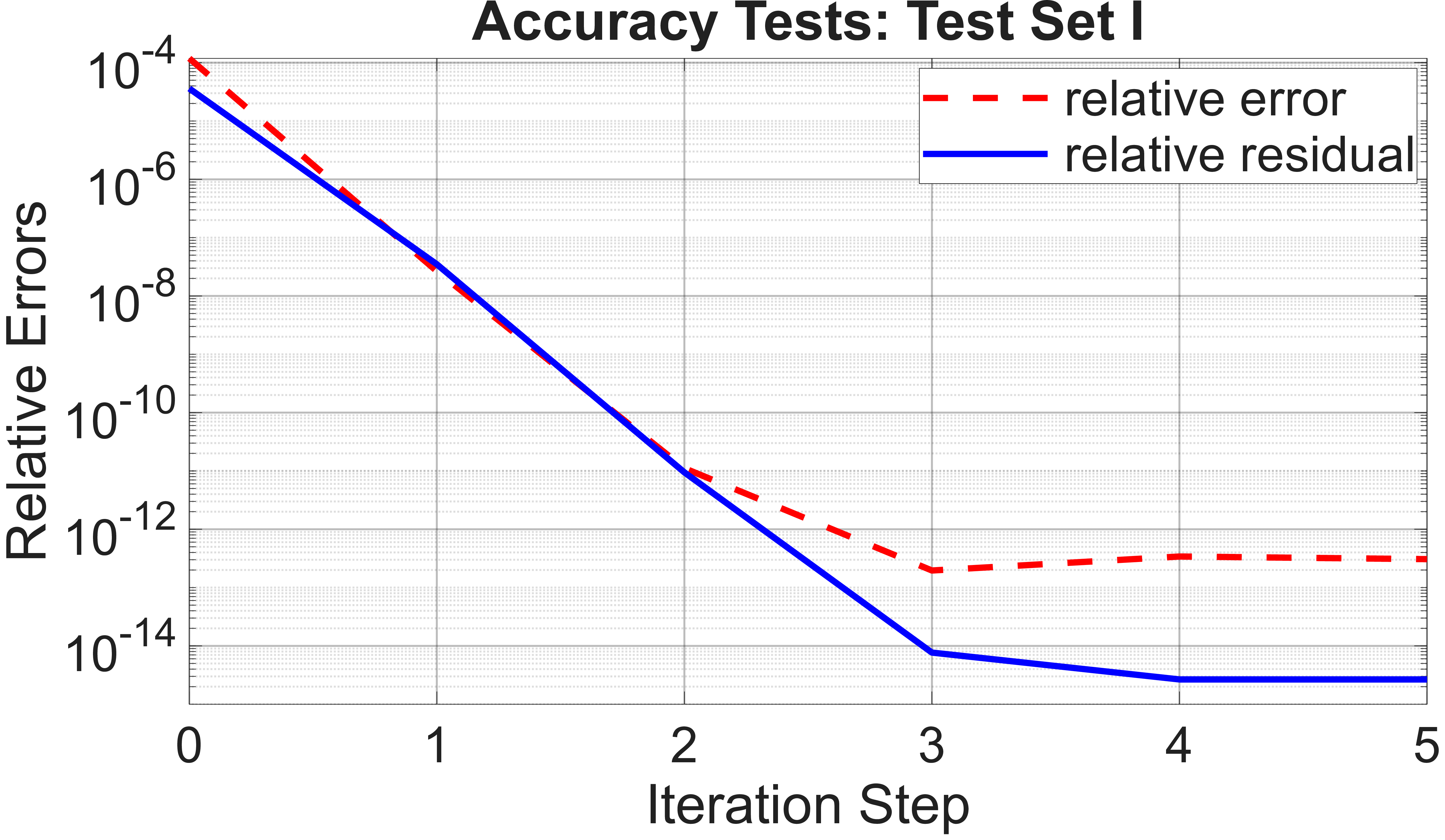
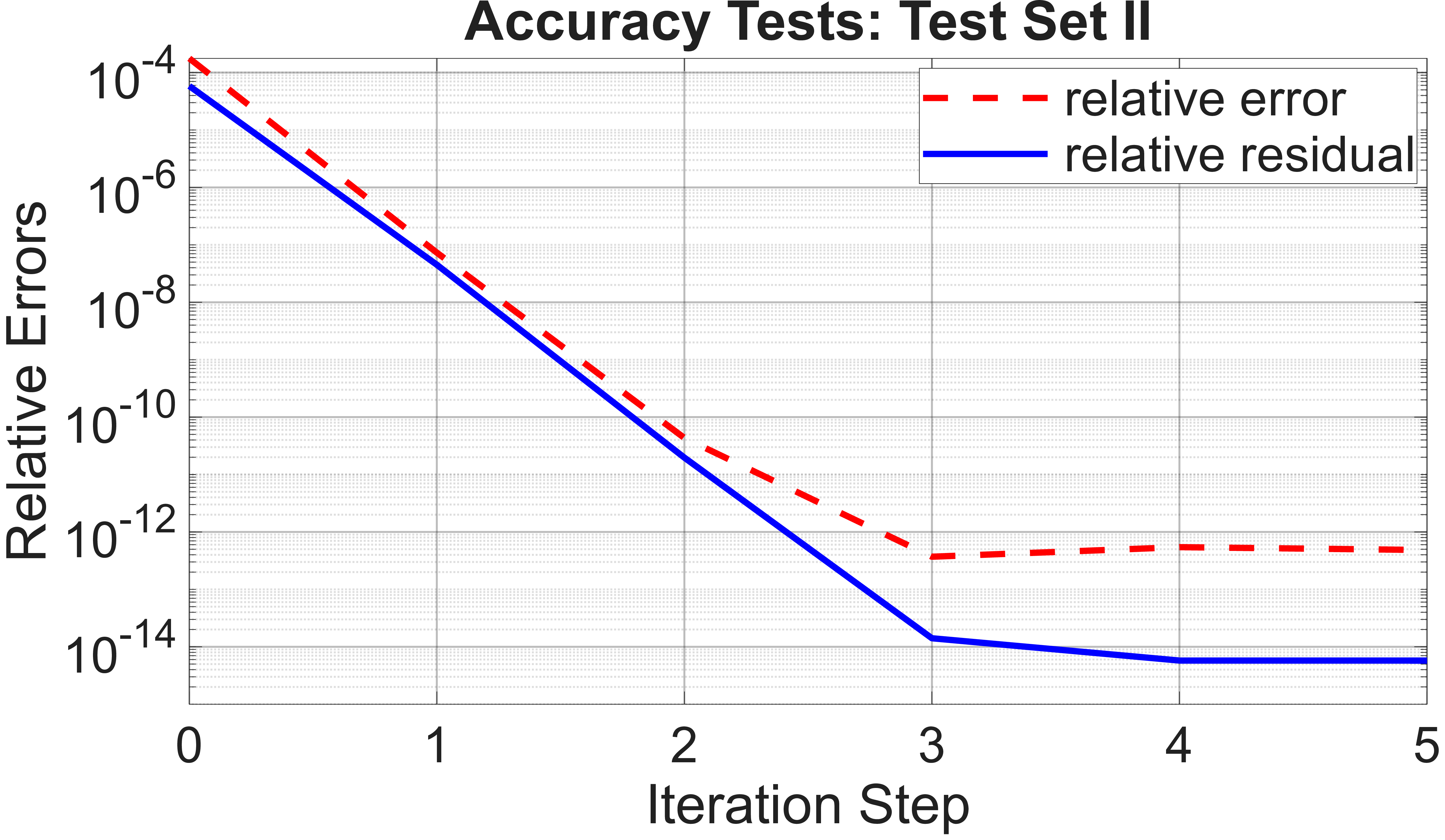
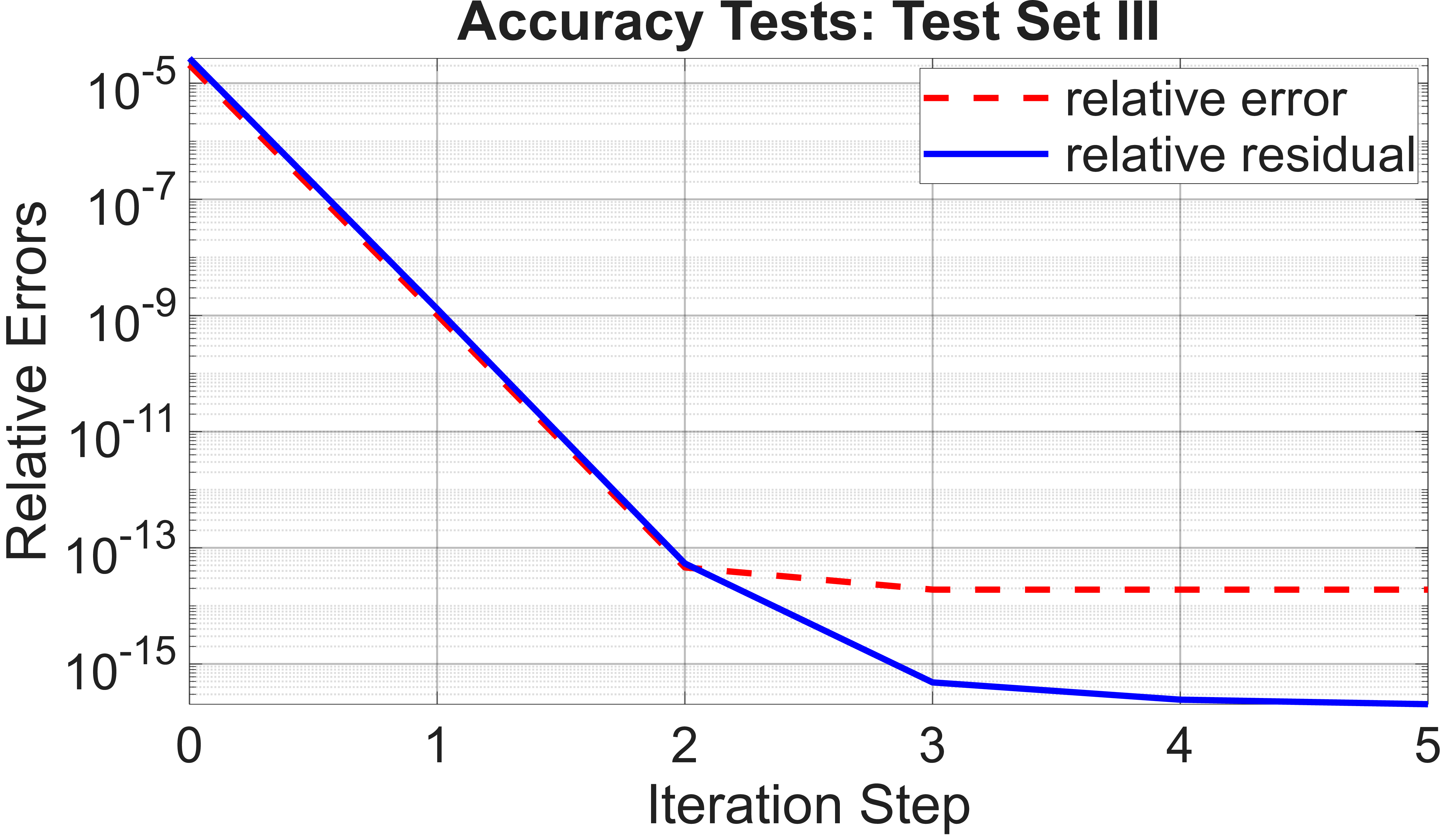

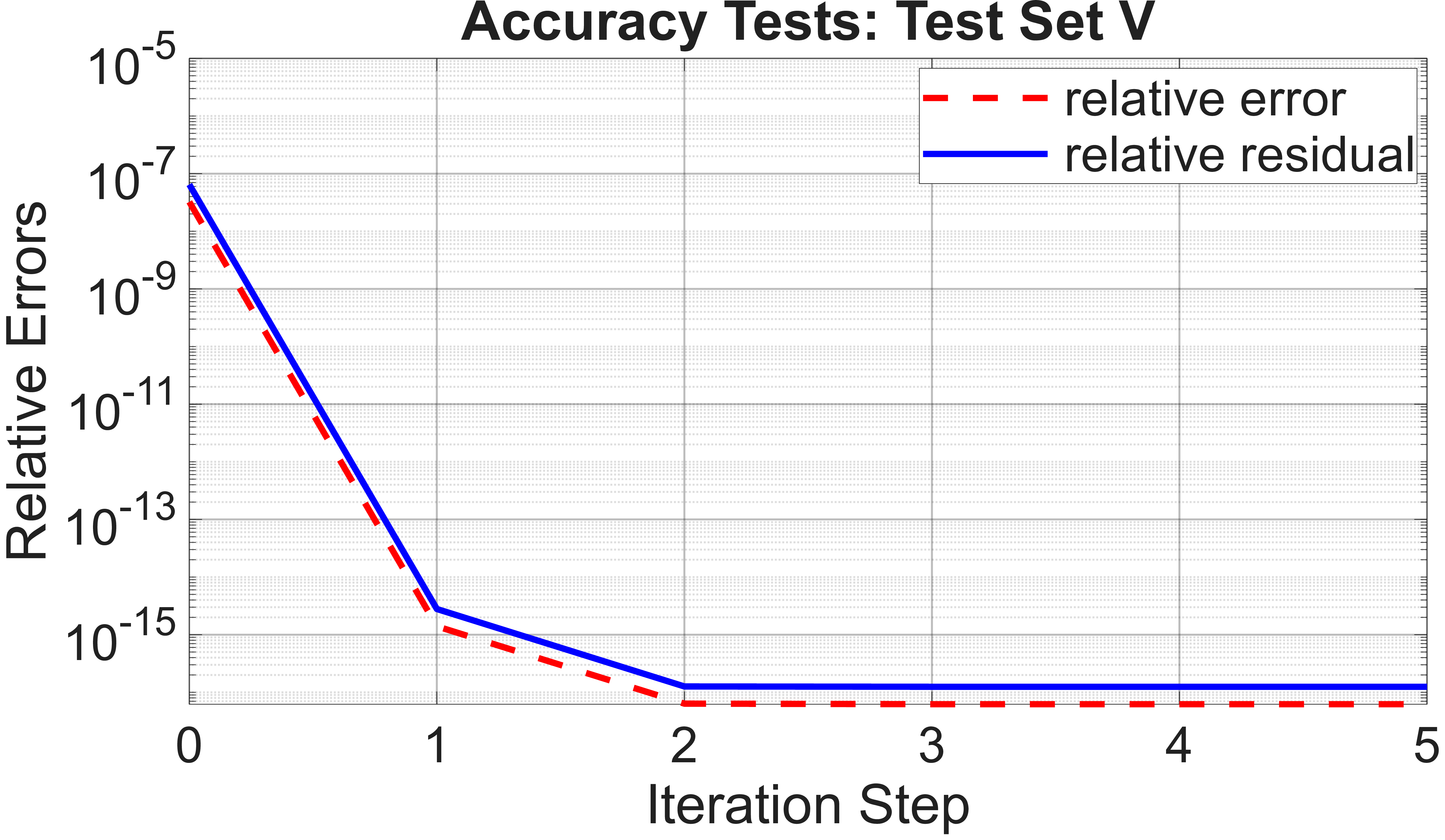
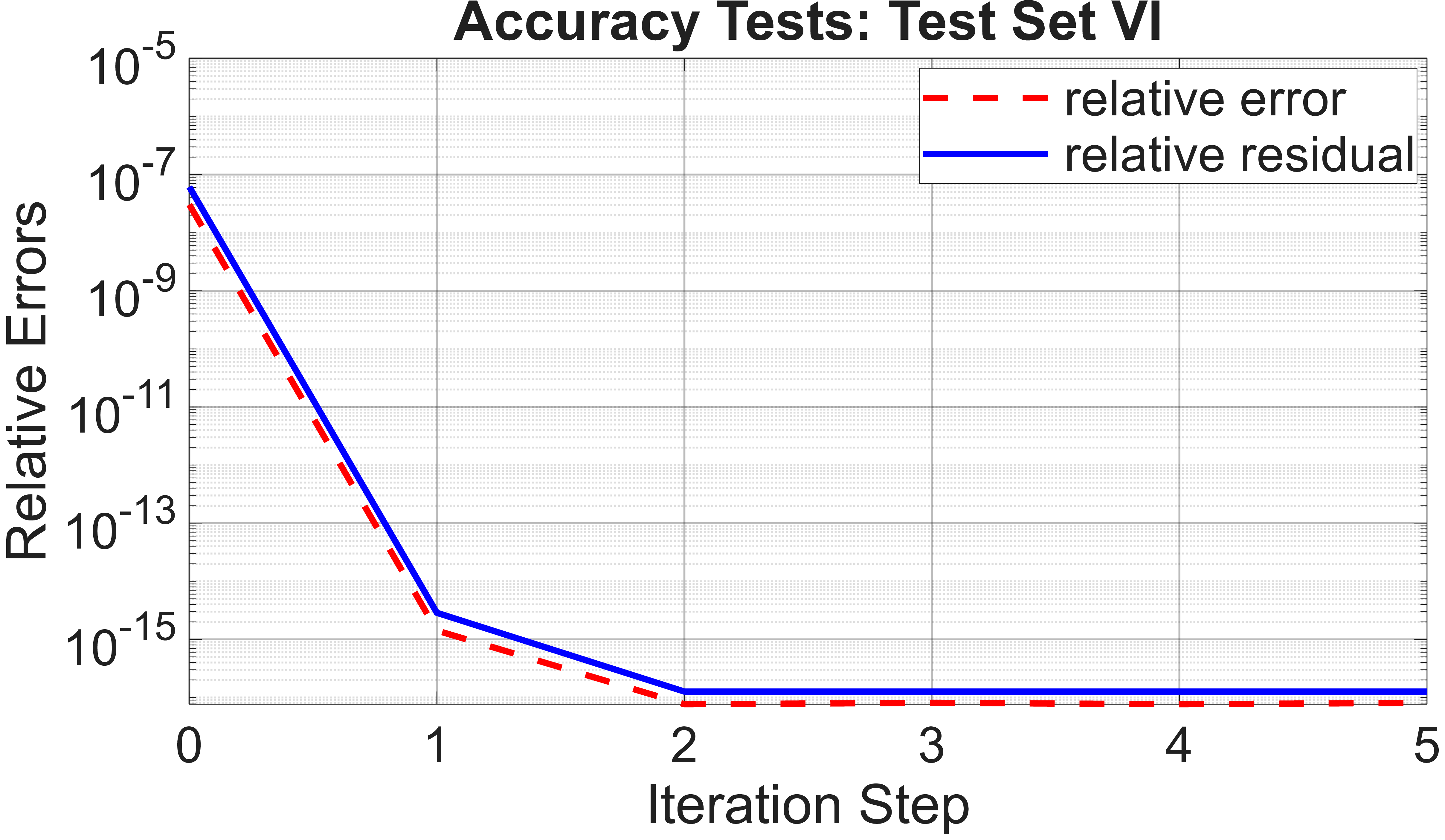
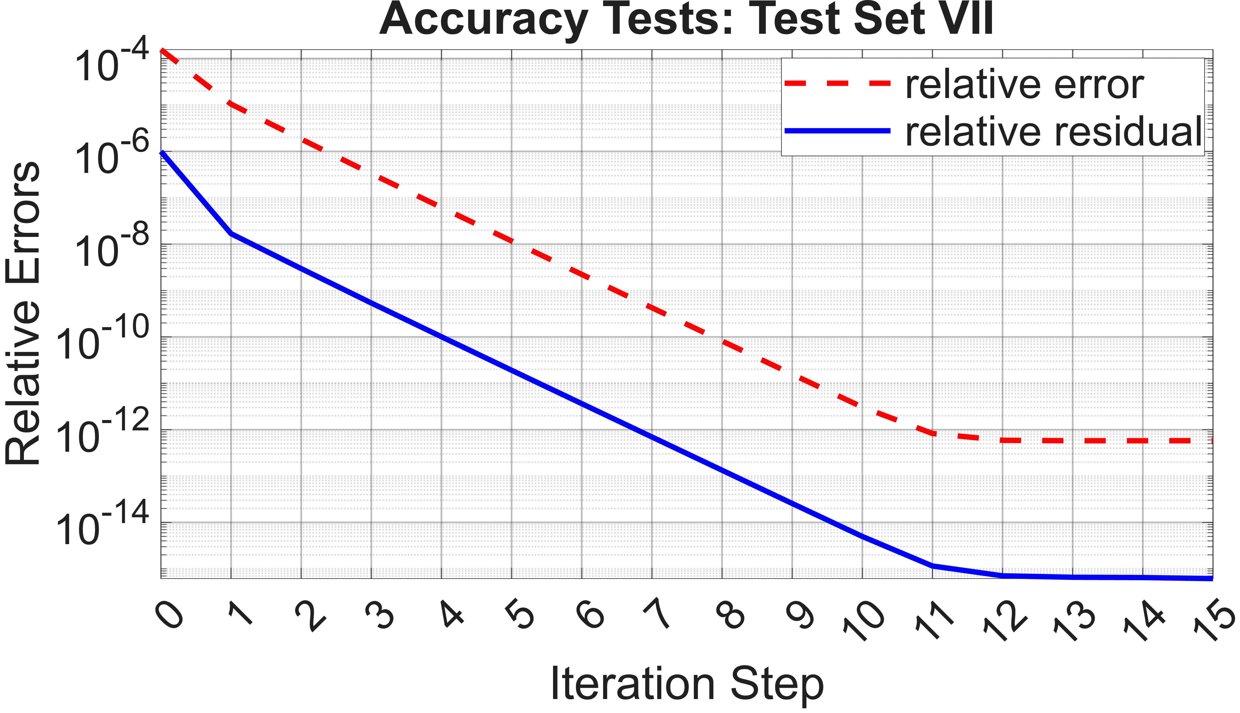
Figure 4: Relative residuals and errors of Algorithms 2 and 3 for computing matrix square roots in mixed precision, with single precision employed as lower precision and double precision employed as working precision. The relative residual is displayed in the solid line, and the relative error is displayed in the dashed line..
From Figure 4, we see that if the matrix is not too ill-conditioned, it only takes 1–3 steps of iterative refinement to reach double precision accuracy. For the highly ill-conditioned Hilbert matrix with a regularization term, our mixed precision algorithm still converges, although it takes around 11–12 steps of iterative refinement. Furthermore, if the regularization factor \(\tau\) is smaller than \(10^{-7}\), it diverges in our tests.
5.2 Performance tests↩︎
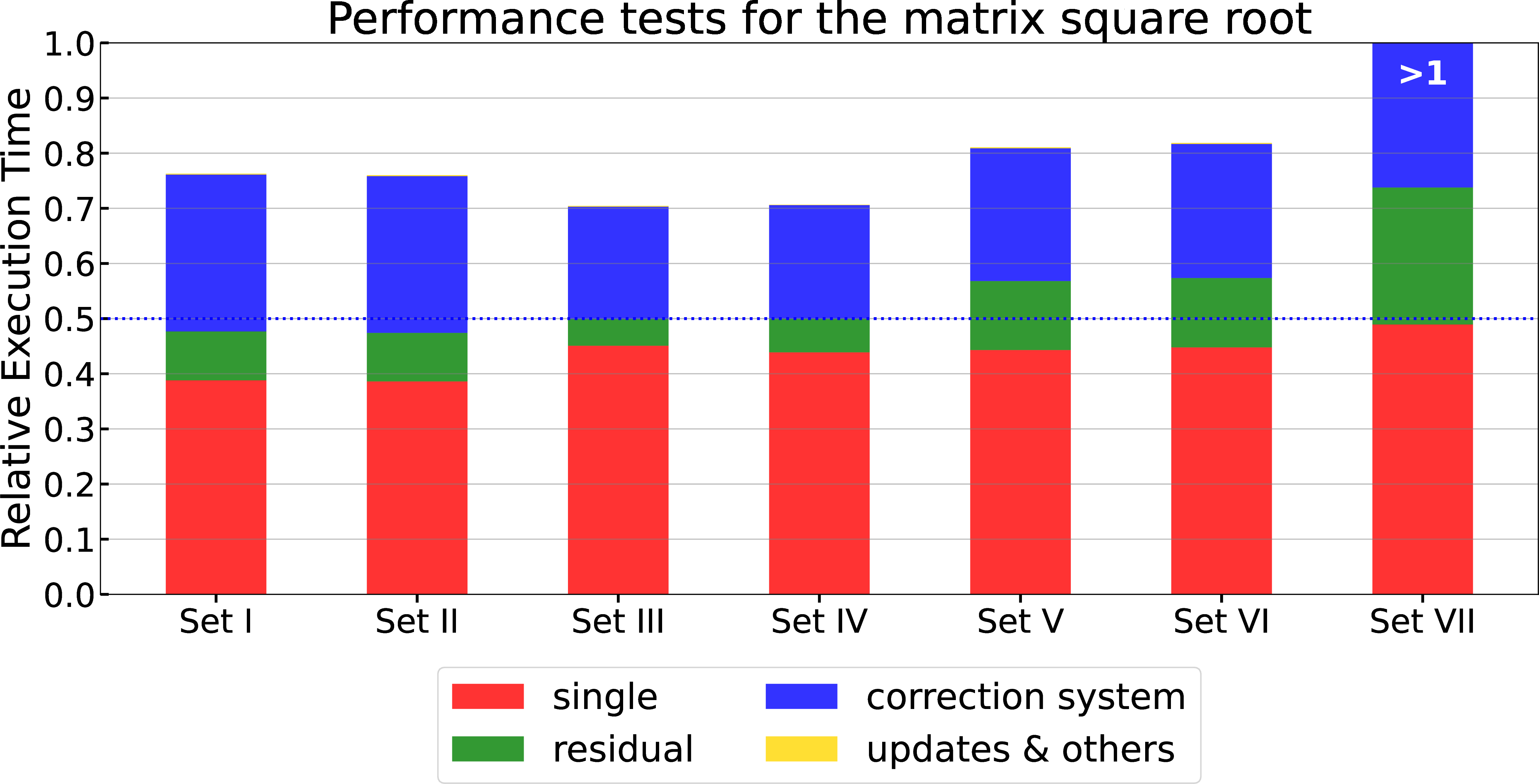
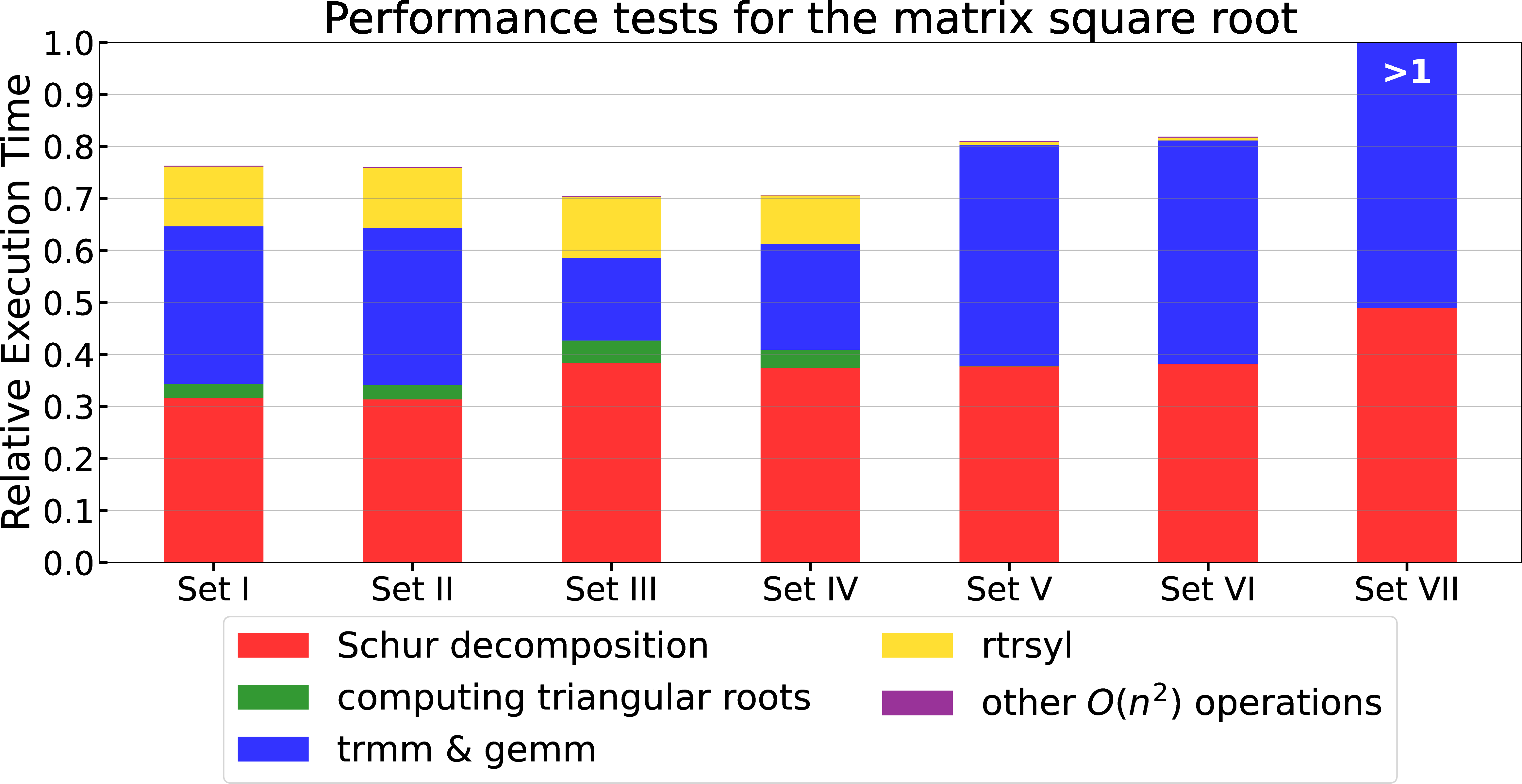
We further test the algorithm performance for the seven sets of matrices. The results are shown in Figures 5 and 6.
In each plot, we record the relative execution time, i.e., the ratio of the wall clock time of the mixed precision solver over that of the double precision Schur algorithm. In Figure 5, we employ labels ‘single’, ‘residual’, ‘correction system’, and ‘updates & others’ to represent the different phases in Algorithms 2 and 3, respectively: computing the initial approximation by the Schur algorithm in single precision, computing the residual in iterative refinement, solving the correction system in iterative refinement, and adding the correction matrix in iterative refinement along with other \(\mathcal{O}(n^{2})\) operations.
In Figure 6, we summarize the execution time by the types of matrix operations in Algorithms 2 and 3. We use labels ‘Schur decomposition’, ‘computing triangular roots’, ‘trmm & gemm’, ‘rtrsyl’, and ‘other \(\mathcal{O}(n^{2})\) operations’ to represent different matrix operations in our algorithms. The results show that the Schur decomposition costs over \(20\)–\(30\) times more than a matrix–matrix multiplication in the same precision, which implies that it is indeed the primary cost and performance impact factor.
For most test matrices, our mixed precision algorithms offer around \(20\%\)–\(30\%\) time savings compared to the fixed (double) precision Schur algorithm, which constitutes a speedup around \(1.2\times\)–\(1.43\times\). For Hilbert matrix with a regularization of \(10^{-6}\), the iterative refinement process is very expensive, and our mixed precision algorithm does not offer any performance gain.
6 Conclusions↩︎
In this paper, we propose a novel mixed precision algorithm for computing matrix square roots. We derive a framework that combines Schur decomposition with iterative refinement to elevate a lower precision approximation to the working precision level. To enhance performance, we incorporate strategies such as reusing Schur factors to obtain an approximate Newton iteration and applying block recursion to solve Sylvester equations. Based on these discussions, we present mixed precision algorithms for computing square roots of both general and symmetric/Hermitian positive definite matrices, as well as an extension to matrix \(p\)th roots.
Convergence analysis demonstrates that our mixed precision algorithms converge at least linearly to the matrix square root when using exact arithmetic. When taking rounding errors into account, we establish that our algorithm for symmetric or Hermitian positive definite matrices recovers an error on the order of the working precision unit-roundoff under mild conditions. We also discuss the generalization of this result to general matrices. Preliminary numerical experiments indicate that our algorithm frequently reduces execution time at a rate of approximately 20–30% compared to the fixed (working) precision Schur algorithm on x86-64 architectures.
Acknowledgement↩︎
The authors thank Yuji Nakatsukasa and Nian Shao for helpful discussions.
References↩︎
University of Manchester, 2022.
School of Data Science, Fudan University, Shanghai 200433, China (, )↩︎
Institute of Mathematics, EPF Lausanne, 1015 Lausanne, Switzerland ()↩︎
Shanghai Key Laboratory for Contemporary Applied Mathematics, Fudan University, Shanghai 200433, China↩︎
Bowen Gao and Meiyue Shao are partially supported by National Key R&D Program of China under Grant No. 2023YFB3001603. Bowen Gao completed part of the work during his visit in EPFL.↩︎