A Fourier-Aware Projection-Based Periodic Parareal Method for Time-Periodic Problems
July 14, 2026
Abstract
Time-periodic problems arise when the desired solution is a periodic steady state rather than a transient trajectory. The periodic parareal algorithm with a periodic coarse problem (PP-PC) is a periodicity-preserving parallel-in-time approach for such problems. Projection-based correction can accelerate convergence of both parareal and PP-PC. In this paper, we propose a Fourier-aware construction of projection spaces and a new correction scheme to further accelerate the convergence of projection-based PP-PC. We develop a convergence analysis of projection-based PP-PC with the discrepancy-based correction scheme for general nonlinear time-periodic problems. For an arbitrary orthogonal projection, we derive a local one-step convergence estimate controlled by the unresolved error and explicit nonlinear contributions. A temporal Fourier decomposition bounds the unresolved error by a tail–leak quantity, which is small when dominant error modes are selected and their coefficients are captured by the projection space. For linear problems, the nonlinear contributions vanish, yielding a globally valid one-step tail–leak convergence estimate under weaker assumptions. Experiments on linear and nonlinear problems show that Fourier-aware PP-PC requires fewer outer iterations than Krylov-enhanced PP-PC. For the linear problems, the errors track the tail–leak bound. For the nonlinear problems, the experiments quantify the unresolved-error and explicit nonlinear contributions in the local one-step estimate and show that the evaluated tail–leak estimate follows the observed decay.
time-periodic problems, parallel-in-time integration, projection-based PP-PC, Fourier-aware projection spaces
65L20, 65L70, 65Y05
1 Introduction↩︎
Time-periodic problems arise naturally in computational models with periodic forcing or cyclic operation, where the quantity of interest is a periodic steady state rather than a transient trajectory. Examples include eddy-current simulations, cyclic chemical processes, and fluid–structure interaction models [1]–[4]. A typical finite-dimensional formulation seeks a function \(\mathbf{u}:\left[0,T\right]\to\mathbb{R}^d\) such that \[\label{eq:intro-periodic-problem} \mathbf{u}'\left(t\right) = \mathbf{f}\left(\mathbf{u}\left(t\right),t\right), \qquad t\in \left[0,T\right], \qquad \mathbf{u}\left(0\right)=\mathbf{u}\left(T\right),\tag{1}\] where \(\mathbf{f}:\mathbb{R}^d\times\mathbb{R}\to\mathbb{R}^d\) satisfies \(\mathbf{f}(\mathbf{x},t+T)=\mathbf{f}(\mathbf{x},t)\) for all \((\mathbf{x},t)\in\mathbb{R}^d\times\mathbb{R}\).
The periodic condition in 1 has been treated by several classes of numerical methods. Frequency-domain formulations exploit periodicity directly, from the classical Galerkin analysis of [5] to harmonic-balance methods for periodic flows [6]. Multigrid methods solve the periodicity-constrained space-time system for time-periodic parabolic problems [7], and waveform-relaxation methods provide an iterative alternative [8]. Shooting and Newton–Picard methods compute periodic states as fixed points of the period map [9], [10].
In large-scale time-domain simulations, spatial parallelism eventually saturates, leaving sequential time propagation as the bottleneck. This has motivated parallel-in-time algorithms that introduce concurrency across time subintervals. Representative parallel-in-time approaches include block boundary-value methods, parareal, PFASST, multigrid-reduction-in-time, and all-at-once time-domain preconditioning methods [11]–[15]; see [16] for a survey. The parareal algorithm realizes this idea through an iterative fine–coarse correction. At each iteration, the fine propagator is applied independently on the time subintervals, and the coarse propagator updates the solution values at the coarse time points. The original parareal method was introduced by Lions, Maday, and Turinici for initial-value problems [17]; see also [18] for its convergence analysis. For time-periodic problems, the periodic condition must be incorporated into the parareal iteration. Gander, Jiang, Song, and Zhang introduced and analyzed a periodic variant [19]: the periodic parareal algorithm with a periodic coarse problem (PP-PC). PP-PC preserves periodicity on the coarse time points at every iteration. However, the PP-PC iteration may converge slowly for oscillatory or wave-like dynamics.
Projection-based correction has been widely used to improve the convergence of parallel-in-time methods. An early time-decomposed framework for implicit parallel-in-time integration was introduced in [20]. Projection has also been used to stabilize parareal iterations for first- and second-order hyperbolic systems [21]. For initial-value problems, the Krylov-enhanced parareal method of [22] improves the iteration through projection. The Krylov-enhanced PP-PC method of [23] extends the Krylov subspace correction to PP-PC, the periodic form of parareal, for time-periodic problems. In these projection-based parareal methods, the projection space determines how fine and coarse propagation are combined, so its choice affects the convergence behavior of the iteration.
In this paper, we introduce a Fourier-aware projection-based PP-PC method, which combines a new correction scheme with a new construction of the projection space. The scheme is discrepancy-based and differs from that of Krylov-enhanced PP-PC. For the projection space, Krylov-enhanced PP-PC uses the full solution-snapshot space, built from the computed solution values over one period. However, Fourier techniques are widely used to exploit temporal structure in time-dependent and time-periodic solvers [14], [24]–[26]. We develop a Fourier-aware construction of the projection space that exploits this structure. The construction represents coarse-time histories in the Fourier basis associated with the coarse-time index. A mode-selection rule specifies which temporal modes to retain. The corresponding modal components are then combined into a mixed Fourier space, which serves as the projection space.
We analyze the convergence of projection-based PP-PC with the discrepancy-based correction scheme for general nonlinear time-periodic problems. The starting point is a local one-step error estimate that holds for a discrepancy-form propagator and an arbitrary projection space, under local smoothness, nondegeneracy, and smallness assumptions. The estimate shows that the error after one iteration is bounded in terms of the unresolved error and two explicit nonlinear contributions. When this unresolved part is represented in temporal Fourier modes, it is bounded by a tail from modes not selected together with a leak from selected modes not fully captured by the projection space. The tail and the leak are both small when the selected set contains the error’s dominant temporal modes and the projection space captures their modal coefficients. Our main result (1) is a Fourier-aware one-step estimate in which the tail–leak form enters the unresolved-error term and the nonlinear remainder, while the base-state term remains unchanged. For linear time-periodic problems, the nonlinear terms vanish; under weaker assumptions, the estimates then reduce exactly to global bounds with the same constants: a general-projection estimate and a tail–leak estimate.
The rest of this paper is organized as follows. 2 recalls PP-PC and presents its projection-based framework. 3 introduces Fourier-aware projection-based PP-PC, its discrepancy-based correction scheme, and its mixed Fourier space. 4 develops the local nonlinear estimate, the Fourier-aware results, and the linear corollaries. 5 reports experiments on two linear and two nonlinear time-periodic problems, and 6 concludes the paper.
2 PP-PC and a framework for its projection-based variants↩︎
In this section we first recall PP-PC and present projection-based PP-PC as a general framework. Then we show that Krylov-enhanced PP-PC is an instance of this framework; our own instance is developed in 3.
2.1 Periodic parareal with a periodic coarse problem↩︎
We begin by recalling the original PP-PC method. Let \[0=T_0<T_1<\cdots<T_N=T, \qquad T_n=n\Delta T,\qquad \Delta T=T/N .\] The points \(T_n\) and the intervals \(\left[T_n,T_{n+1}\right]\) are called the coarse time points and coarse time intervals, respectively. The solution values at the coarse time points are called the interface values. They are vectors in a real finite-dimensional state space, denoted by \(\mathbb{R}^d\). At iteration \(k\) the interface values are \[\mathbf{U}^k = \left(\mathbf{U}_0^k,\ldots,\mathbf{U}_{N-1}^k\right) \in\left(\mathbb{R}^d\right)^N .\] The periodic condition identifies the endpoint value with the initial value: \[\mathbf{U}_N^k=\mathbf{U}_0^k .\]
The PP-PC method is built from a fine propagator and a coarse propagator on each coarse time interval. For \(0\le n<N\) and \(\mathbf{x}\in\mathbb{R}^d\), let \[\mathcal{F}\left(T_{n+1},T_n,\mathbf{x}\right), \qquad \mathcal{G}\left(T_{n+1},T_n,\mathbf{x}\right)\] denote the corresponding fine and coarse propagator values over \(\left[T_n,T_{n+1}\right]\), respectively, starting from the state \(\mathbf{x}\) at \(T_n\). More precisely, if \(\mathbf{u}\left(\cdot;T_n,\mathbf{x}\right)\) denotes the solution of the underlying evolution problem satisfying \(\mathbf{u}\left(T_n;T_n,\mathbf{x}\right)=\mathbf{x}\), then \(\mathcal{F}\left(T_{n+1},T_n,\mathbf{x}\right)\) gives an accurate approximation of \(\mathbf{u}\left(T_{n+1};T_n,\mathbf{x}\right)\). The coarse propagator \(\mathcal{G}\left(T_{n+1},T_n,\mathbf{x}\right)\) gives a less accurate but less expensive approximation of the same state. When no ambiguity arises, we write \[\mathcal{F}_n\left(\mathbf{x}\right):=\mathcal{F}\left(T_{n+1},T_n,\mathbf{x}\right), \qquad \mathcal{G}_n\left(\mathbf{x}\right):=\mathcal{G}\left(T_{n+1},T_n,\mathbf{x}\right).\]
The PP-PC iteration [19] computes \(\mathbf{U}^{k+1}\) from \(\mathbf{U}^k\) by \[\label{eq:pppc-expanded} \begin{align} \mathbf{U}_0^{k+1} &= \mathcal{F}_{N-1}\left(\mathbf{U}_{N-1}^k\right) + \mathcal{G}_{N-1}\left(\mathbf{U}_{N-1}^{k+1}\right) - \mathcal{G}_{N-1}\left(\mathbf{U}_{N-1}^k\right),\\ \mathbf{U}_{n+1}^{k+1} &= \mathcal{F}_n\left(\mathbf{U}_n^k\right) + \mathcal{G}_n\left(\mathbf{U}_n^{k+1}\right) - \mathcal{G}_n\left(\mathbf{U}_n^k\right), \qquad n=0,\ldots,N-2 . \end{align}\tag{2}\] Once \(\mathbf{U}^k\) is known, the fine and coarse propagator evaluations at \(\mathbf{U}_n^k\) are available. These fine propagator evaluations are independent across the coarse time intervals and can therefore be performed in parallel. The new values \(\mathbf{U}_n^{k+1}\) remain coupled through the terms \(\mathcal{G}_n\left(\mathbf{U}_n^{k+1}\right)\). The first equation closes the cycle by coupling \(\mathbf{U}_0^{k+1}\) to \(\mathbf{U}_{N-1}^{k+1}\). This coupled solve is the periodic coarse problem in PP-PC.
2.2 A framework for projection-based PP-PC↩︎
In PP-PC the correction in 2 is carried by the coarse propagator \(\mathcal{G}_n\). Projection-based PP-PC generalizes this step. At iteration \(k\) it constructs a projection space \(\mathcal{V}^k\subset\mathbb{R}^d\), with orthogonal projection \(P^k\) onto it, and replaces \(\mathcal{G}_n\) in the correction by a projection-based propagator \(\mathcal{X}_{P^k,n}\). It computes \(\mathbf{U}^{k+1}\) from the coupled periodic problem \[\label{eq:projection-corrected-pppc} \begin{align} \mathbf{U}_0^{k+1} &= \mathcal{F}_{N-1}\left(\mathbf{U}_{N-1}^k\right) + \mathcal{X}_{P^k,N-1}\left(\mathbf{U}_{N-1}^{k+1}\right) - \mathcal{X}_{P^k,N-1}\left(\mathbf{U}_{N-1}^k\right),\\ \mathbf{U}_{n+1}^{k+1} &= \mathcal{F}_n\left(\mathbf{U}_n^k\right) + \mathcal{X}_{P^k,n}\left(\mathbf{U}_n^{k+1}\right) - \mathcal{X}_{P^k,n}\left(\mathbf{U}_n^k\right), \qquad n=0,\ldots,N-2 . \end{align}\tag{3}\] Taking \(\mathcal{X}_{P,n}=\mathcal{G}_n\) recovers PP-PC 2 . The framework leaves two ingredients to be specified: the projection space \(\mathcal{V}^k\) and the projection-based propagator \(\mathcal{X}_{P^k,n}\). Different choices give different methods, while the structure of the iteration is unchanged. Once \(P^k\) and \(\mathcal{X}_{P^k,n}\) are fixed, the values \(\mathcal{F}_n(\mathbf{U}_n^k)\) and \(\mathcal{X}_{P^k,n}(\mathbf{U}_n^k)\) at the known iterate are independent across the coarse intervals and are computed in parallel; the new values \(\mathbf{U}_n^{k+1}\) remain coupled only through \(\mathcal{X}_{P^k,n}(\mathbf{U}_n^{k+1})\), and the first equation closes the cycle. 1 summarizes the framework.
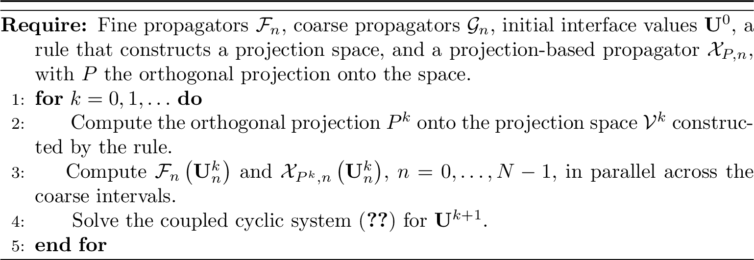
Krylov-enhanced PP-PC [23] is an instance of this framework. For initial-value problems, the Krylov-enhanced parareal method [22] accelerates parareal by a projection built from solution snapshots; the periodic version applies the same idea to PP-PC. Its projection space is the full solution-snapshot space \[\label{eq:krylov-snapshot-space} \mathcal{V}_{\rm K}^k := \mathop{\mathrm{span}}\left\{\,\mathbf{U}_n^j:\;0\le j\le k,\;0\le n<N\,\right\},\tag{4}\] which in the present periodic notation collects all interface values available up to iteration \(k\). Let \(P_{\rm K}^k\) be the orthogonal projection onto \(\mathcal{V}_{\rm K}^k\) and set \(Q_{\rm K}^k:=I-P_{\rm K}^k\), where \(I\) is the identity matrix on \(\mathbb{R}^d\). Its projection-based propagator is the split form \[\label{eq:krylov-enhanced-propagator} \mathcal{K}_{{\rm K},n}^k\left(\mathbf{x}\right) := \mathcal{F}_n\left(P_{\rm K}^k\mathbf{x}\right) + \mathcal{G}_n\left(Q_{\rm K}^k\mathbf{x}\right),\tag{5}\] which applies the fine propagator on the snapshot space and the coarse propagator on its complement. Krylov-enhanced PP-PC is therefore 1 with the projection space of step [line:gen-proj] set to the snapshot space \(\mathcal{V}_{\rm K}^k\) and the projection-based propagator of step [line:gen-solve] to the split form \(\mathcal{K}_{{\rm K},n}^k\); equivalently, the iteration 3 with \(\mathcal{X}_{P^k,n}=\mathcal{K}_{{\rm K},n}^k\).
3 Fourier-aware projection-based PP-PC↩︎
Under the framework of 2.2, our method makes two new choices: a discrepancy-based correction scheme and a Fourier-aware projection space. This correction scheme is realized by the discrepancy-form propagator, the precise object we define first.
Definition 1 (Discrepancy-form propagator). Let \(P:\mathbb{R}^d\to\mathbb{R}^d\) be an arbitrary orthogonal projection. For \(0\le n<N\), the fine–coarse discrepancy on the coarse time interval \(\left[T_n,T_{n+1}\right]\) is defined by \[\label{eq:discrepancy-map} \mathcal{D}_n\left(\mathbf{x}\right):=\mathcal{F}_n\left(\mathbf{x}\right)-\mathcal{G}_n\left(\mathbf{x}\right),\qquad{(1)}\] and the discrepancy-form propagator associated with \(P\) is defined by \[\label{eq:discrepancy-form-propagator} \mathcal{H}_{P,n}\left(\mathbf{x}\right) := \mathcal{G}_n\left(\mathbf{x}\right)+\mathcal{D}_n\left(P\mathbf{x}\right) = \mathcal{G}_n\left(\mathbf{x}\right) +\mathcal{F}_n\left(P\mathbf{x}\right) -\mathcal{G}_n\left(P\mathbf{x}\right).\qquad{(2)}\]
The propagator \(\mathcal{H}_{P,n}\) is not a coarse propagator. It adds to the coarse value \(\mathcal{G}_n(\mathbf{x})\) the fine–coarse discrepancy evaluated at the projected state \(P\mathbf{x}\); projection-based PP-PC with this propagator is 3 with \(\mathcal{X}_{P^k,n}=\mathcal{H}_{P^k,n}\).
The remaining choice is the projection space, the central algorithmic issue in projection-based PP-PC. Because the discrepancy-form propagator applies fine–coarse information only to the projected component, a projection space is useful to the extent that it captures the components that the iteration still has to correct. For time-periodic problems these components have temporal structure that the discrete Fourier transform (DFT) in the coarse-time index makes explicit.
At iteration \(k\), the interface values \[\mathbf{U}^k = \left(\mathbf{U}_0^k,\ldots,\mathbf{U}_{N-1}^k\right)\] form the solution history over one period. Its temporal Fourier coefficients are \[\label{eq:temporal-fourier-coefficients} \widehat{\mathbf{U}}_\ell^k = \frac{1}{\sqrt N} \sum_{n=0}^{N-1} \mathbf{U}_n^k \exp\left(-2\pi \imath\ell n/N\right), \qquad \ell=0,\ldots,N-1.\tag{6}\] The same transform applies to any coarse-time history. Here \(\imath\) is the imaginary unit. The index \(\ell\) represents a temporal Fourier mode, with phase increment \(2\pi\ell/N\) on the coarse time grid. For low positive indices the corresponding physical angular frequency is \(2\pi\ell/T\); indices near \(N\) represent the negative frequencies \(2\pi(\ell-N)/T\). The coefficient \(\widehat{\mathbf{U}}_\ell^k\) is the content of the solution history in that mode. For notational simplicity we identify a mode with its index \(\ell\), so that a set of temporal Fourier modes is a subset of \(\{0,\ldots,N-1\}\).
The mode \(\ell=0\) is the mean component over the period. Modes with small positive indices describe slowly varying components on the cyclic coarse time grid. Thus the coefficients \(\widehat{\mathbf{U}}_\ell^k\) describe how the solution history is distributed among temporal frequencies of the periodic iteration. Truncated Fourier representations have proved effective in several time-periodic applications [1], [6]. The construction exploits temporal concentration when it is present: a mode-selection rule first chooses the temporally relevant modes (3.1), and the projection space is then built from the modal components of the solution and the fine–coarse discrepancy histories at the selected modes (3.2).
3.1 Selection of temporal modes↩︎
The Fourier-aware construction first chooses a selected temporal mode set. At iteration \(k\), the selected temporal mode set is denoted by \[\mathcal{I}^k\subset\left\{0,\ldots,N-1\right\}.\] When only a few temporal modes carry significant content, the construction aims to retain those modes. Convergence may degrade if the selected set omits a mode carrying a significant part of the current error. The two choices below correspond to two practical regimes:
The fixed choice applies when the dominant temporal frequencies of the response are known in advance. It then uses the same prescribed mode set at every iteration, \[\mathcal{I}^k=\mathcal{I}_{\mathrm{fix}}\quad\text{for all } k, \qquad \mathcal{I}_{\mathrm{fix}}\subset\left\{0,\ldots,N-1\right\},\] with \(\mathcal{I}_{\mathrm{fix}}\) the modes at those frequencies. It is appropriate when the periodic response is dominated by low temporal frequencies, for which we take \(\mathcal{I}_{\mathrm{fix}}\) to be the symmetric low-frequency band \[\label{eq:low-frequency-band} \mathcal{I}_L = \left\{0,1,\ldots,L\right\}\cup\left\{N-L,\ldots,N-1\right\}, \qquad 1\le L<N/2 .\tag{7}\] This band retains the mean mode and the first \(L\) positive temporal frequencies together with their negative-frequency counterparts.
The adaptive increment-energy choice applies when the dominant temporal frequencies are not known in advance, or change during the iteration. It uses the current iteration increment. For \(k\ge 1\), set \[\Delta \mathbf{U}_n^k = \mathbf{U}_n^k-\mathbf{U}_n^{k-1}.\] Let \(\widehat{\Delta\mathbf{U}}_\ell^k\) be its temporal Fourier coefficients and define \[\label{eq:increment-energy} a_\ell^k = \left\|\widehat{\Delta\mathbf{U}}_\ell^k\right\|_2^2, \qquad \ell=0,\ldots,N-1.\tag{8}\] Since the histories are real, \(a_\ell^k=a_{(N-\ell)\bmod N}^k\), so the energies are properties of the conjugate groups \(\{\ell,(N-\ell)\bmod N\}\). The adaptive rule ranks these groups by their combined energy and retains the \(M\) highest-ranked groups, where \(M\) is a prescribed number. The mode \(\ell=0\) is self-conjugate, as is \(\ell=N/2\) when \(N\) is even, so the selected set \(\mathcal{I}^k\) contains at most \(2M\) modes. For \(k=0\) no increment is available; we set \(\mathcal{I}^0=\emptyset\), so the first update reduces to the PP-PC step. The increment estimates the iteration error: for a contracting iteration, \(\Delta\mathbf{U}^k\) is dominated by the error still to be removed, so its leading temporal modes follow those of the error. This link is heuristic: for a noncontracting or oscillatory iteration the temporal spectrum of \(\Delta\mathbf{U}^k\) need not match that of the error, and the adequacy of the selection is assessed a posteriori in 5.
3.2 Construction of the Fourier-aware projection space↩︎
A selected mode affects the correction only through its modal components in the projection space. The construction of the projection space is guided by the role of \(P\) in the projection-based PP-PC update 3 and in the discrepancy-form propagator ?? . For an orthogonal projection \(P\) and the current solution history \(\mathbf{U}^k\), define the correction source \[\mathbf{c}_{n+1}^k\left(P\right) := \mathcal{F}_n\left(\mathbf{U}_n^k\right) - \mathcal{H}_{P,n}\left(\mathbf{U}_n^k\right), \qquad n=0,\ldots,N-1 .\] By the definition of \(\mathcal{H}_{P,n}\), this source is \[\mathbf{c}_{n+1}^k\left(P\right) = \mathcal{D}_n\left(\mathbf{U}_n^k\right) - \mathcal{D}_n\left(P\mathbf{U}_n^k\right).\] With the discrepancy-form propagator, the projection-based PP-PC step is the cyclic system—its operator matrix understood rowwise, as made precise below— \[\label{eq:cyclic-system} \begin{bmatrix} I& 0 & \cdots & -\mathcal{H}_{P,N-1}\left(\cdot\right)\\ -\mathcal{H}_{P,0}\left(\cdot\right) & I& & 0\\ \vdots & \ddots & \ddots & \vdots\\ 0 & \cdots & -\mathcal{H}_{P,N-2}\left(\cdot\right) & I \end{bmatrix} \begin{bmatrix} \mathbf{U}_0^{k+1}\\ \mathbf{U}_1^{k+1}\\ \vdots\\ \mathbf{U}_{N-1}^{k+1} \end{bmatrix} = \begin{bmatrix} \mathbf{c}_N^k\left(P\right)\\ \mathbf{c}_1^k\left(P\right)\\ \vdots\\ \mathbf{c}_{N-1}^k\left(P\right) \end{bmatrix}.\tag{9}\] We refer to the operator on the left-hand side as the cyclic operator associated with \(\mathcal{H}_{P,n}\), and denote it by \(\mathcal{C}_P\). Throughout, indices of histories are read modulo \(N\), so that \(\mathcal{C}_P\) acts rowwise as \(\left(\mathcal{C}_P\mathbf{w}\right)_{n+1}=\mathbf{w}_{n+1}-\mathcal{H}_{P,n}(\mathbf{w}_n)\), \(n=0,\ldots,N-1\). The projection acts at the states where the discrepancy-form propagator is evaluated and in the correction source \(\mathbf{c}_{n+1}^k\left(P\right)\); the projection space should therefore be informed by both the solution and the fine–coarse discrepancy histories:
The solution histories contain those evaluation states \(\mathbf{U}_n^m\); their selected modal components identify state-space directions associated with the retained temporal content of the periodic iterates.
The discrepancy histories contain the correction directions \(\mathbf{d}_n^m=\mathcal{D}_n\left(\mathbf{U}_n^m\right)\); since \(\mathbf{c}_{n+1}^k\left(P\right)\) compares \(\mathcal{D}_n\left(\mathbf{U}_n^k\right)\) with \(\mathcal{D}_n\left(P\mathbf{U}_n^k\right)\), they identify the discrepancy components the projection should capture.
The projection space is therefore built from both histories. The one-step estimate in 4 contains a projection-dependent source contribution obtained by applying a local fine–coarse discrepancy bound to the unresolved part of the current error. A cyclic stability factor also enters the estimate, together with two additional contributions in the nonlinear case.
For each \(0\le m\le k\) and \(\ell=0,\ldots,N-1\), the solution history \(\mathbf{U}^m\) and the fine–coarse discrepancy history \(\mathbf{d}^m\) have temporal Fourier coefficients \[\label{eq:solution-discrepancy-dft} \widehat{\mathbf{U}}_\ell^m = \frac{1}{\sqrt N}\sum_{n=0}^{N-1}\mathbf{U}_n^m \exp\left(-2\pi\imath\ell n/N\right), \quad \widehat{\mathbf{d}}_\ell^m = \frac{1}{\sqrt N}\sum_{n=0}^{N-1}\mathbf{d}_n^m \exp\left(-2\pi\imath\ell n/N\right).\tag{10}\] These coefficients are complex in general, whereas the projection space is a subspace of \(\mathbb{R}^d\); we therefore take their real and imaginary parts, omitting any that vanish. The selected modal components of the solution history span the solution-generated Fourier space \[\label{eq:solution-generated-fourier-space} \mathcal{V}_{\rm sol}^k\left(\mathcal{I}^k\right) := \mathop{\mathrm{span}}\left\{ \operatorname{Re}\widehat{\mathbf{U}}_\ell^m, \operatorname{Im}\widehat{\mathbf{U}}_\ell^m: \ell\in\mathcal{I}^k,\;0\le m\le k \right\}\tag{11}\] and those of the fine–coarse discrepancy history span the discrepancy-generated Fourier space \[\label{eq:discrepancy-generated-fourier-space} \mathcal{V}_{\rm disc}^k\left(\mathcal{I}^k\right) := \mathop{\mathrm{span}}\left\{ \operatorname{Re}\widehat{\mathbf{d}}_\ell^m, \operatorname{Im}\widehat{\mathbf{d}}_\ell^m: \ell\in\mathcal{I}^k,\;0\le m\le k \right\}.\tag{12}\] The Fourier-aware projection space is their sum, the mixed Fourier space \[\label{eq:mixed-fourier-projection-space} \mathcal{V}_{\rm mix}^k\left(\mathcal{I}^k\right) := \mathcal{V}_{\rm sol}^k\left(\mathcal{I}^k\right) + \mathcal{V}_{\rm disc}^k\left(\mathcal{I}^k\right).\tag{13}\] It is the smallest subspace containing both, so a single projection \(P\) onto \(\mathcal{V}_{\rm mix}^k\left(\mathcal{I}^k\right)\) captures the selected modal components of the evaluation states and of the discrepancy directions entering the correction source.
Remark 1. Since the DFT 6 is an invertible linear transform in the coarse-time index and the histories are real, the real span of \(\{\operatorname{Re}\widehat{\mathbf{U}}_\ell^m, \operatorname{Im}\widehat{\mathbf{U}}_\ell^m:0\le\ell<N\}\) equals the span of \(\{\mathbf{U}_n^m:0\le n<N\}\) for each \(m\). With all temporal modes selected, the solution-generated Fourier space is therefore exactly the full solution-snapshot space: \(\mathcal{V}_{\rm sol}^k(\{0,\ldots,N-1\})=\mathcal{V}_{\rm K}^k\).
3.3 The Fourier-aware projection-based PP-PC algorithm↩︎
We now combine these ingredients into Fourier-aware projection-based PP-PC. At each iteration \(k\), choose the selected temporal mode set \(\mathcal{I}^k\) by one of the rules in 3.1. The projection space is the mixed Fourier space \(\mathcal{V}_{\rm mix}^k\left(\mathcal{I}^k\right)\) of 13 , and \(P_{\mathcal{I}^k}\) is the orthogonal projection onto it. The Fourier-aware projection-based PP-PC update is the periodic solve 3 with the discrepancy-form propagator and \(P^k=P_{\mathcal{I}^k}\), namely \[\label{eq:fourier-aware-pppc} \begin{align} \mathbf{U}_0^{k+1} &= \mathcal{F}_{N-1}\left(\mathbf{U}_{N-1}^k\right) + \mathcal{H}_{P_{\mathcal{I}^k},N-1}\left(\mathbf{U}_{N-1}^{k+1}\right) - \mathcal{H}_{P_{\mathcal{I}^k},N-1}\left(\mathbf{U}_{N-1}^k\right),\\ \mathbf{U}_{n+1}^{k+1} &= \mathcal{F}_n\left(\mathbf{U}_n^k\right) + \mathcal{H}_{P_{\mathcal{I}^k},n}\left(\mathbf{U}_n^{k+1}\right) - \mathcal{H}_{P_{\mathcal{I}^k},n}\left(\mathbf{U}_n^k\right), \qquad n=0,\ldots,N-2 . \end{align}\tag{14}\] 2 summarizes the procedure. Its main parameter is the band width \(L\) of the fixed rule or the mode count \(M\) of the adaptive rule; the experimental values are given in 5. In an implementation, past Fourier coefficients are stored, so only those of the newly generated solution and fine–coarse discrepancy histories are computed at iteration \(k\).
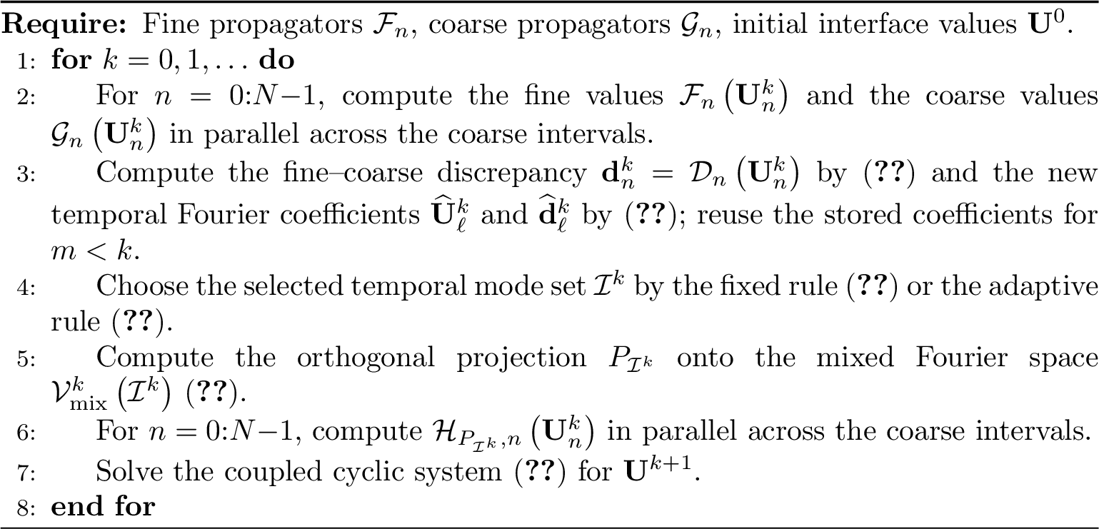
The discrepancy-form propagator \(\mathcal{H}_{P,n}(\mathbf{x})=\mathcal{G}_n(\mathbf{x})+\mathcal{D}_n(P\mathbf{x})\) evaluates the fine propagator at the projected state \(P\mathbf{x}\). In the corrected update 14 this evaluation falls on the next iterate \(\mathbf{U}^{k+1}\), the unknown of the cyclic system 9 , so the cost of the correction depends on how that system is solved. For affine \(\mathcal{F}_n\) and \(\mathcal{G}_n\) the cyclic system is linear. Its operator is assembled from the fine propagator applied to the projection basis, and the correction is a single linear solve with no further fine propagations; the fine propagator is otherwise evaluated only at the current iterate \(\mathbf{U}^k\), in parallel across the coarse intervals as in the original PP-PC.
Remark 2 (Distinction from Krylov-enhanced PP-PC). Fourier-aware PP-PC and Krylov-enhanced PP-PC are two instances of the projection-based framework 1; they fix its two free ingredients—the projection space of step [line:gen-proj] and the projection-based propagator of step [line:gen-solve]—differently. For the projection space, Fourier-aware PP-PC builds the mixed Fourier space \(\mathcal{V}_{\rm mix}^k\left(\mathcal{I}^k\right)\) 13 , whereas Krylov-enhanced PP-PC uses the full solution-snapshot space \(\mathcal{V}_{\rm K}^k\) 4 . For the propagator, the difference is more fundamental and independent of the space choice: Krylov-enhanced PP-PC uses the split-form propagator \[\mathcal{F}_n\left(P\mathbf{x}\right) + \mathcal{G}_n\left(\left(I-P\right)\mathbf{x}\right),\] whereas Fourier-aware PP-PC uses the discrepancy-form propagator \[\mathcal{H}_{P,n}\left(\mathbf{x}\right) = \mathcal{G}_n\left(\mathbf{x}\right) + \left(\mathcal{F}_n-\mathcal{G}_n\right)\left(P\mathbf{x}\right).\] In the affine case the two forms differ only by a constant: if \(\mathcal{G}_n\) is affine, then for every \(\mathbf{x}\) \[\mathcal{H}_{P,n}(\mathbf{x})-\mathcal{F}_n(P\mathbf{x})-\mathcal{G}_n\left(\left(I-P\right)\mathbf{x}\right) = \mathcal{G}_n(\mathbf{x})-\mathcal{G}_n(P\mathbf{x})-\mathcal{G}_n\left(\left(I-P\right)\mathbf{x}\right) = -\mathcal{G}_n(\mathbf{0}),\] and this constant cancels between the two evaluations of the propagator in the update 14 , so the corresponding iterations produce identical iterates; the distinction is therefore active only in the nonlinear regime.
4 Error and convergence analysis↩︎
This section analyzes the error and convergence of projection-based PP-PC with our discrepancy-based correction scheme, realized by the discrepancy-form propagator ?? . The analysis considers the general nonlinear time-periodic problem \[\label{eq:nonlinear-periodic-problem} \mathbf{u}'(t)=\mathbf{f}(\mathbf{u}(t),t), \qquad t\in[0,T], \qquad \mathbf{u}(0)=\mathbf{u}(T),\tag{15}\] where \(\mathbf{f}(\mathbf{x},t+T)=\mathbf{f}(\mathbf{x},t)\) for all \(\mathbf{x}\) in a domain containing the states considered below.
Throughout, \(\mathrm D\) denotes the Jacobian of a map with respect to the state, the subscript \(\mathbf{u}\) marking the partial Jacobian of \(\mathbf{f}(\mathbf{u},t)\) in its state argument; \(\mathbf{f}\) and \(\mathrm D_{\mathbf{u}}\mathbf{f}\) are assumed continuous in \((\mathbf{u},t)\). Let \(\mathbf{u}^\star_{\mathrm c}\) denote a \(T\)-periodic solution, assumed to exist; the subscript marks the continuous-time solution. Linearizing 15 about \(\mathbf{u}^\star_{\mathrm c}\) gives the variational equation \[\label{eq:floquet-variational} \dot{\mathbf{v}}=A_\star(t)\,\mathbf{v}, \qquad A_\star(t):=\mathrm D_{\mathbf{u}}\mathbf{f}\!\left(\mathbf{u}^\star_{\mathrm c}(t),t\right),\tag{16}\] a linear system with \(T\)-periodic coefficients. Let its fundamental matrix \(\Phi\) satisfy \(\dot{\Phi}=A_\star\Phi\) and \(\Phi(0)=I\). Then \(\mathbf{v}(T)=\Phi(T)\mathbf{v}(0)\), where \(\Phi(T)\) is the monodromy matrix, whose eigenvalues are the Floquet multipliers [10], [27], [28].
Assumption 1 (Nondegenerate periodic solution). The periodic solution \(\mathbf{u}^\star_{\mathrm c}\) is nondegenerate: no Floquet multiplier equals \(1\), equivalently the variational equation has no nontrivial \(T\)-periodic solution.
Define the period map \(\varphi_T(\mathbf{x}):=\mathbf{u}(T;\mathbf{x})\), where \(\mathbf{u}(0;\mathbf{x})=\mathbf{x}\). Since \(\mathrm D\varphi_T(\mathbf{u}^\star_{\mathrm c}(0))=\Phi(T)\) and \(I-\Phi(T)\) is invertible by 1, the implicit function theorem implies that \(\mathbf{u}^\star_{\mathrm c}(0)\) is locally unique among the fixed points of \(\varphi_T\). If the fine period map \(\Phi_{\mathcal{F}}:=\mathcal{F}_{N-1}\circ\cdots\circ\mathcal{F}_0\) converges to \(\varphi_T\) in \(C^1\) near \(\mathbf{u}^\star_{\mathrm c}(0)\), then for sufficiently small fine steps \(\Phi_{\mathcal{F}}\) has a locally unique fixed point \(\mathbf{u}_0^\star\) near \(\mathbf{u}^\star_{\mathrm c}(0)\). This fixed point is nondegenerate: \(I-\mathrm D\Phi_{\mathcal{F}}(\mathbf{u}_0^\star)\) is invertible. We thus define the fine periodic reference \[\label{eq:fine-periodic-reference} \mathbf{u}^\star = \left(\mathbf{u}_0^\star,\ldots,\mathbf{u}_{N-1}^\star\right) \in \left(\mathbb{R}^d\right)^N,\tag{17}\] by the fine-propagator interface equations \[\label{eq:fine-periodic-reference-interface} \mathbf{u}_{n+1}^\star=\mathcal{F}_n\left(\mathbf{u}_n^\star\right), \qquad n=0,\ldots,N-1, \qquad \mathbf{u}_N^\star=\mathbf{u}_0^\star .\tag{18}\] The preceding argument gives a sufficient condition for the existence of this discrete reference. The estimates below assume its existence and measure the iteration error of \(\mathbf{U}^k\) relative to it. The error at the coarse time points is \[\mathbf{e}_n^k:=\mathbf{u}_n^\star-\mathbf{U}_n^k, \qquad n=0,\ldots,N-1,\] its maximum-in-time size is \[E_\infty^k:=\max_{0\le n<N}\left\lVert \mathbf{e}_n^k \right\rVert_2 ,\] and the error history is \[\mathbf{e}^k:=\left(\mathbf{e}_0^k,\ldots,\mathbf{e}_{N-1}^k\right) \in\left(\mathbb{R}^d\right)^N .\] On histories \(\mathbf{w}=(\mathbf{w}_0,\ldots,\mathbf{w}_{N-1})\in(\mathbb{R}^d)^N\) we use the maximum-in-time norm and the operator norm it induces, \[\left\lVert \mathbf{w} \right\rVert_\infty:=\max_{0\le n<N}\left\lVert \mathbf{w}_n \right\rVert_2 , \qquad \left\lVert S \right\rVert_{\infty\to\infty}:=\sup_{\mathbf{w}\neq\mathbf{0}}\frac{\left\lVert S\mathbf{w} \right\rVert_\infty}{\left\lVert \mathbf{w} \right\rVert_\infty} ,\] so that \(E_\infty^k=\left\lVert \mathbf{e}^k \right\rVert_\infty\). History indices are taken modulo \(N\); in particular, \(\mathbf{U}_N^{k+1}=\mathbf{U}_0^{k+1}\), \(\mathbf{u}_N^\star=\mathbf{u}_0^\star\), and \(\mathbf{e}_N^{k+1}=\mathbf{e}_0^{k+1}\). For one projection-based PP-PC update, fix an arbitrary projection space \(\mathcal{V}\subset\mathbb{R}^d\), let \(P\) be its orthogonal projection, and set \(Q:=I-P\). We call \(Q\mathbf{w}=(Q\mathbf{w}_0,\ldots,Q\mathbf{w}_{N-1})\in(\mathbb{R}^d)^N\) the unresolved part of \(\mathbf{w}\). The local one-step estimate uses three assumptions.
Assumption 2 (Local nonlinear region). Fix an iteration index \(k\) and write \(P:=P^k\). There exists a convex set \(\mathcal{B}_k\subset\mathbb{R}^d\) such that, for all \(n=0,\ldots,N-1\) and \(s\in[0,1]\), \[\mathbf{U}_n^k+s\mathbf{e}_n^k\in\mathcal{B}_k, \qquad P(\mathbf{U}_n^k+s\mathbf{e}_n^k)\in\mathcal{B}_k, \qquad \mathbf{u}_n^\star,\mathbf{U}_n^{k+1}\in\mathcal{B}_k .\] We also assume that \(\mathcal{H}_{P,n}\) is well defined on \(\mathcal{B}_k\).
Assumption 3 (Local nondegeneracy). Under 2, each \(\mathcal{H}_{P^k,n}\) is continuously differentiable on an open neighborhood of \(\mathcal{B}_k\). The linearized cyclic operator \(\widehat{\mathcal{C}}_{P^k}\), obtained by linearizing the cyclic operator \(\mathcal{C}_{P^k}\) of 9 at \(\mathbf{u}^\star\), acts on a periodic history \(\mathbf{w}\) by \[\left(\widehat{\mathcal{C}}_{P^k}\mathbf{w}\right)_{n+1} := \mathbf{w}_{n+1} - \mathrm D\mathcal{H}_{P^k,n}(\mathbf{u}_n^\star)\mathbf{w}_n, \quad n=0,\ldots,N-1, \quad \mathbf{w}_N=\mathbf{w}_0 .\] The matrix \[\widehat M_{P^k}:=\mathrm D\mathcal{H}_{P^k,N-1}(\mathbf{u}_{N-1}^\star)\cdots \mathrm D\mathcal{H}_{P^k,0}(\mathbf{u}_0^\star)\] is the monodromy of the linearized cyclic system. We assume this linearization is nondegenerate: \(1\notin\sigma(\widehat M_{P^k})\). By the cyclic recurrence, this is equivalent to the invertibility of \(\widehat{\mathcal{C}}_{P^k}\). We set \[\label{eq:nonlinear-Gamma-definition} \widehat\Gamma_k:=\left\lVert \widehat{\mathcal{C}}_{P^k}^{-1} \right\rVert_{\infty\to\infty}.\qquad{(3)}\] This condition concerns the linearization of \(\mathcal{H}_{P^k,n}\) at the fine reference and is not implied by 1.
Assumption 4 (Local smoothness). Under the setting of 2, suppose that each \(\mathcal{D}_n\) is continuously Fréchet differentiable on an open neighborhood of \(\mathcal{B}_k\). There exist constants \(\mu_k\ge 0\) and \(\nu_k\ge 0\) such that, for all \(\mathbf{x},\mathbf{y}\in\mathcal{B}_k\) and \(n=0,\ldots,N-1\), \[\label{eq:nonlinear-discrepancy-smoothness} \left\lVert \mathrm D\mathcal{D}_n(\mathbf{x}) \right\rVert_2\le \mu_k, \qquad \left\lVert \mathrm D\mathcal{D}_n(\mathbf{x})-\mathrm D\mathcal{D}_n(\mathbf{y}) \right\rVert_2 \le \nu_k\left\lVert \mathbf{x}-\mathbf{y} \right\rVert_2 .\qquad{(4)}\] Suppose in addition that the projection-based propagators \(\mathcal{H}_{P,n}\) have Lipschitz Jacobians on \(\mathcal{B}_k\): for some constant \(\kappa_k\ge0\), \[\label{eq:nonlinear-corrected-curvature} \left\lVert \mathrm D\mathcal{H}_{P,n}(\mathbf{x})-\mathrm D\mathcal{H}_{P,n}(\mathbf{y}) \right\rVert_2 \le \kappa_k\left\lVert \mathbf{x}-\mathbf{y} \right\rVert_2, \qquad \mathbf{x},\mathbf{y}\in\mathcal{B}_k .\qquad{(5)}\] The constants \(\mu_k\), \(\nu_k\), \(\kappa_k\) are associated with the local set \(\mathcal{B}_k\), which itself depends on the iterate and the projection through 2.
The following additional assumption is used only in the contractive special case discussed in 5.
Assumption 5 (Coarse-propagator contraction). There exists a constant \(L_G>0\), independent of the coarse time interval index \(n\) and of \(\Delta T\), such that the coarse propagator satisfies the uniform contraction bound \[\left\lVert \mathcal{G}_n\left(\mathbf{x}\right)-\mathcal{G}_n\left(\mathbf{y}\right) \right\rVert_2 \le \frac{1}{1+L_G\Delta T}\left\lVert \mathbf{x}-\mathbf{y} \right\rVert_2,\] for \(n=0,\ldots,N-1\) and all \(\mathbf{x},\mathbf{y}\in\mathbb{R}^d\).
4.1 Projection-dependent one-step analysis↩︎
For one update of 3 using the discrepancy-form propagator with \(P^k=P\), define the unresolved fine–coarse discrepancy \[\label{eq:nonlinear-unresolved-correction} \mathcal{R}_{P,n}(\mathbf{x}) := \mathcal{F}_n(\mathbf{x})-\mathcal{H}_{P,n}(\mathbf{x}) = \mathcal{D}_n(\mathbf{x})-\mathcal{D}_n(P\mathbf{x}).\tag{19}\] If \(E_\infty^k>0\), define the unresolved-error ratio \(\theta_Q^k(P)\) and the projected-error ratio \(\theta_P^k(P)\) by \[\theta_Q^k(P) := \frac{\max_{0\le n<N}\left\lVert Q\mathbf{e}_n^k \right\rVert_2}{E_\infty^k}, \qquad \theta_P^k(P) := \frac{\max_{0\le n<N}\left\lVert P\mathbf{e}_n^k \right\rVert_2}{E_\infty^k},\] and define the base-state weight by \[U_k^\perp(P) := \max_{0\le n<N}\left\lVert Q\mathbf{U}_n^k \right\rVert_2 .\] The next lemma combines these quantities in the projection-dependent factor \(\rho_k(P)\).
Lemma 1 (Projection-dependent local one-step convergence estimate). For the nonlinear problem 15 , let \(\mathbf{u}^\star\) be the fine periodic reference in 17 . Suppose that [ass:local-nonlinear-neighborhood,ass:local-nonlinear-nondegeneracy,ass:local-discrepancy-smoothness] hold at iteration \(k\) for the orthogonal projection \(P\). Assume also that, for some \(R>0\), the update \(\mathbf{U}^{k+1}\) satisfies \(E_\infty^{k+1}\le R\) and the smallness condition \[\label{eq:nonlinear-smallness} \tfrac12\widehat\Gamma_k\kappa_kR<1.\qquad{(6)}\] If \(E_\infty^k=0\), then \(E_\infty^{k+1}=0\). If \(E_\infty^k>0\), then the projection-based PP-PC update 3 using the discrepancy-form propagator with \(P^k=P\) satisfies \[\label{eq:local-nonlinear-projection-estimate} E_\infty^{k+1} \le \rho_k(P)E_\infty^k,\qquad{(7)}\] where \[\label{eq:local-nonlinear-one-step-factor} \rho_k(P) := \frac{\widehat\Gamma_k}{1-\tfrac12\widehat\Gamma_k\kappa_kR} \left[ \mu_k\theta_Q^k(P) + \nu_kU_k^\perp(P)\theta_P^k(P) + \frac{\nu_k}{2} \theta_Q^k(P)\theta_P^k(P)E_\infty^k \right].\qquad{(8)}\]
Proof. By the update 3 using the discrepancy-form propagator with \(P^k=P\), the iterate \(\mathbf{U}^{k+1}\) satisfies \[\mathbf{U}_{n+1}^{k+1} = \mathcal{F}_n(\mathbf{U}_n^k) + \mathcal{H}_{P,n}(\mathbf{U}_n^{k+1}) - \mathcal{H}_{P,n}(\mathbf{U}_n^k), \qquad n=0,\ldots,N-1 .\] For \(n=N-1\), the equality is interpreted with \(\mathbf{U}_N^{k+1}=\mathbf{U}_0^{k+1}\) and \(\mathbf{u}_N^\star=\mathbf{u}_0^\star\), so that \(\mathbf{e}_N^{k+1}=\mathbf{e}_0^{k+1}\). Subtracting this identity from 18 and using \[\mathcal{F}_n(\mathbf{x}) = \mathcal{H}_{P,n}(\mathbf{x})+\mathcal{R}_{P,n}(\mathbf{x}),\] we obtain \[\label{eq:nonlinear-corrected-error-equation} \mathbf{e}_{n+1}^{k+1} = \bigl[ \mathcal{H}_{P,n}(\mathbf{u}_n^\star) - \mathcal{H}_{P,n}(\mathbf{U}_n^{k+1}) \bigr] + \bigl[ \mathcal{R}_{P,n}(\mathbf{u}_n^\star) - \mathcal{R}_{P,n}(\mathbf{U}_n^k) \bigr] .\tag{20}\] By 3 each \(\mathcal{H}_{P,n}\) is differentiable; writing \(\mathbf{U}_n^{k+1}=\mathbf{u}_n^\star-\mathbf{e}_n^{k+1}\), a Taylor expansion at the reference with the curvature bound ?? gives \[\label{eq:nonlinear-first-bracket-linearization} \mathcal{H}_{P,n}(\mathbf{u}_n^\star)-\mathcal{H}_{P,n}(\mathbf{U}_n^{k+1}) = \mathrm D\mathcal{H}_{P,n}(\mathbf{u}_n^\star)\,\mathbf{e}_n^{k+1}+\boldsymbol{\eta}_n, \qquad \left\lVert \boldsymbol{\eta}_n \right\rVert_2\le\frac{\kappa_k}{2}\left\lVert \mathbf{e}_n^{k+1} \right\rVert_2^2 .\tag{21}\] It remains to estimate \(\mathcal{R}_{P,n}(\mathbf{u}_n^\star)-\mathcal{R}_{P,n}(\mathbf{U}_n^k)\). Write \(\mathbf{U}=\mathbf{U}_n^k\), \(\mathbf{e}=\mathbf{e}_n^k\), and \(\mathcal{D}=\mathcal{D}_n\). For \(s\in[0,1]\), set \[\mathbf{z}_s:=\mathbf{U}+s\mathbf{e}, \qquad \boldsymbol{\zeta}_s:=P\mathbf{z}_s .\] Thus \(\boldsymbol{\zeta}_s=P\mathbf{U}+sP\mathbf{e}\). By 2, both paths lie in \(\mathcal{B}_k\). Using \[\mathcal{R}_{P,n}(\mathbf{x}) = \mathcal{D}_n(\mathbf{x})-\mathcal{D}_n(P\mathbf{x})\] and the fundamental theorem of calculus along the two paths, \[\begin{align} \mathcal{R}_{P,n}(\mathbf{u}_n^\star)-\mathcal{R}_{P,n}(\mathbf{U}_n^k) &= \int_0^1 \left[ \mathrm D\mathcal{D}(\mathbf{z}_s)\mathbf{e} - \mathrm D\mathcal{D}(\boldsymbol{\zeta}_s)P\mathbf{e} \right]ds \\ &= \int_0^1 \mathrm D\mathcal{D}(\mathbf{z}_s)Q\mathbf{e}\,ds + \int_0^1 \left[ \mathrm D\mathcal{D}(\mathbf{z}_s)-\mathrm D\mathcal{D}(\boldsymbol{\zeta}_s) \right] P\mathbf{e}\,ds . \end{align}\] The first integral is bounded by \(\mu_k\left\lVert Q\mathbf{e}_n^k \right\rVert_2\). For the second one, ?? gives \[\left\lVert \mathrm D\mathcal{D}(\mathbf{z}_s)-\mathrm D\mathcal{D}(\boldsymbol{\zeta}_s) \right\rVert_2 \le \nu_k\left\lVert \mathbf{z}_s-\boldsymbol{\zeta}_s \right\rVert_2 .\] Moreover, \(\mathbf{z}_s-\boldsymbol{\zeta}_s = Q\mathbf{U}_n^k+sQ\mathbf{e}_n^k\). Therefore \[\int_0^1\left\lVert \mathbf{z}_s-\boldsymbol{\zeta}_s \right\rVert_2\,ds \le \left\lVert Q\mathbf{U}_n^k \right\rVert_2 + \frac{1}{2}\left\lVert Q\mathbf{e}_n^k \right\rVert_2 .\] Hence integration in \(s\) gives \[\label{eq:nonlinear-unresolved-bound} \left\lVert \mathcal{R}_{P,n}(\mathbf{u}_n^\star)-\mathcal{R}_{P,n}(\mathbf{U}_n^k) \right\rVert_2 \le \mu_k\left\lVert Q\mathbf{e}_n^k \right\rVert_2 + \nu_k\left\lVert Q\mathbf{U}_n^k \right\rVert_2 \left\lVert P\mathbf{e}_n^k \right\rVert_2 + \frac{\nu_k}{2} \left\lVert Q\mathbf{e}_n^k \right\rVert_2 \left\lVert P\mathbf{e}_n^k \right\rVert_2 .\tag{22}\] Substituting 21 into 20 shows that the error history \(\mathbf{e}^{k+1}\) solves the cyclic system \[\widehat{\mathcal{C}}_{P^k}\,\mathbf{e}^{k+1}=\mathbf{s}^k+\boldsymbol{\eta}, \qquad \mathbf{s}_{n+1}^k:=\mathcal{R}_{P,n}(\mathbf{u}_n^\star)-\mathcal{R}_{P,n}(\mathbf{U}_n^k),\] with indices modulo \(N\). Here \(\mathbf{s}^k\) is the unresolved source history. The history \(\boldsymbol{\eta}\) has blocks \((\boldsymbol{\eta})_{n+1}:=\boldsymbol{\eta}_n\), with \(\boldsymbol{\eta}_n\) from 21 . By the same equation, \(\left\lVert \boldsymbol{\eta} \right\rVert_\infty\le\tfrac{\kappa_k}{2}\left(E_\infty^{k+1}\right)^2\). Since \(\widehat{\mathcal{C}}_{P^k}\) is invertible, \[E_\infty^{k+1} \le \widehat\Gamma_k\left( \left\lVert \mathbf{s}^k \right\rVert_\infty+\tfrac{\kappa_k}{2}\left(E_\infty^{k+1}\right)^2 \right),\] while 22 , maximized over \(n\), bounds the unresolved source by \[\begin{align} \left\lVert \mathbf{s}^k \right\rVert_\infty \le{}& \mu_k\max_{0\le n<N}\left\lVert Q\mathbf{e}_n^k \right\rVert_2 +\nu_kU_k^\perp(P)\max_{0\le n<N}\left\lVert P\mathbf{e}_n^k \right\rVert_2\\ &+\frac{\nu_k}{2}\max_{0\le n<N}\left\lVert Q\mathbf{e}_n^k \right\rVert_2\max_{0\le n<N}\left\lVert P\mathbf{e}_n^k \right\rVert_2 . \end{align}\] If \(E_\infty^k=0\), then \(\mathbf{s}^k=\mathbf{0}\), so \(E_\infty^{k+1}\le\tfrac12\widehat\Gamma_k\kappa_kR\,E_\infty^{k+1}\) by \(E_\infty^{k+1}\le R\), and the smallness condition ?? forces \(E_\infty^{k+1}=0\). Otherwise, using \(\left(E_\infty^{k+1}\right)^2\le R\,E_\infty^{k+1}\) and ?? , \[\left(1-\tfrac12\widehat\Gamma_k\kappa_kR\right)E_\infty^{k+1} \le \widehat\Gamma_k\left\lVert \mathbf{s}^k \right\rVert_\infty;\] dividing by \(E_\infty^k\) and using the definitions of \(\theta_Q^k(P)\), \(\theta_P^k(P)\), and \(U_k^\perp(P)\) gives ?? . ◻
Remark 3. The factor \(\rho_k(P)\) is the nonlinear counterpart of the one-step PP-PC factor in [19]. It may vary with \(k\) because both the projection and the local constants may change. The three bracketed contributions in ?? are the unresolved-error term \(\mu_k\theta_Q^k(P)\), the base-state term \(\nu_kU_k^\perp(P)\theta_P^k(P)\), and the discrepancy-curvature remainder \(\tfrac{\nu_k}{2}\theta_Q^k(P)\theta_P^k(P)E_\infty^k\). If \(P=0\), then \[\theta_Q^k(0)=1,\qquad \theta_P^k(0)=0,\qquad \rho_k(0)= \frac{\widehat\Gamma_k\mu_k}{1-\tfrac12\widehat\Gamma_k\kappa_kR},\] the local linearized analogue of the discrepancy-Lipschitz PP-PC factor. If \(P=I\), then \(\theta_Q^k(I)=U_k^\perp(I)=0\), so \(\rho_k(I)=0\), consistently with \(\mathcal{H}_{I,n}=\mathcal{F}_n\).
Remark 4. The local assumptions are tailored to the discrepancy form, which evaluates \(\mathcal{G}_n\) at \(\mathbf{x}\) and \(\mathcal{D}_n\) at \(P\mathbf{x}\), both covered by \(\mathcal{B}_k\). The split form 5 additionally evaluates \(\mathcal{G}_n\) at \(Q\mathbf{x}\), which need not belong to \(\mathcal{B}_k\) and would require regularity at those additional states. Since the fine propagator enters only through \(\mathcal{D}_n\), no contraction of it is required.
Remark 5. Coarse-propagator contraction together with a small discrepancy is sufficient for the nondegeneracy condition in 3. Indeed, [ass:propagator-contraction,ass:local-discrepancy-smoothness] give \[\mathrm D\mathcal{H}_{P,n}(\mathbf{u}_n^\star) = \mathrm D\mathcal{G}_n(\mathbf{u}_n^\star) + \mathrm D\mathcal{D}_n(P\mathbf{u}_n^\star)P, \qquad \left\lVert \mathrm D\mathcal{H}_{P,n}(\mathbf{u}_n^\star) \right\rVert_2 \le \alpha_k:=\frac{1}{1+L_G\Delta T}+\mu_k ,\] since \(P\mathbf{u}_n^\star\in\mathcal{B}_k\) (2 with \(s=1\)) and \(P\) is nonexpansive. If \(\alpha_k<1\), a Neumann-series argument gives \(\widehat\Gamma_k\le(1-\alpha_k)^{-1}\), and 1 yields \[\label{eq:local-nonlinear-contraction-factor} E_\infty^{k+1} \le \rho_k^{\alpha}(P)E_\infty^k, \rho_k^{\alpha}(P) := \frac{\mu_k\theta_Q^k(P)+\nu_kU_k^\perp(P)\theta_P^k(P) +\tfrac{\nu_k}{2}\theta_Q^k(P)\theta_P^k(P)E_\infty^k}{(1-\alpha_k)-\tfrac12\kappa_kR},\qquad{(9)}\] provided \(\tfrac12\kappa_kR<1-\alpha_k\), which also implies ?? .
When the discrepancy admits the local expansion \(\mathcal{D}_n(\mathbf{x})=\boldsymbol{\psi}_{n,p+1}(\mathbf{x})(\Delta T)^{p+1} +\mathbf{r}_n(\mathbf{x})\), with \(p\ge1\) the order of the coarse propagator and, uniformly in \(n\), \(\boldsymbol{\psi}_{n,p+1}\) bounded in \(C^{1,1}\) and \(\mathbf{r}_n=O((\Delta T)^{p+2})\) in the \(C^{1,1}\) sense, one has \(\mu_k,\nu_k=O((\Delta T)^{p+1})\). If, in addition, \(\mathcal{G}_n(\mathbf{x})=\mathbf{x}+\Delta T\,\mathbf{g}_n(\mathbf{x}) +O(\Delta T^2)\) in \(C^{1,1}\), with \(\mathbf{g}_n\) uniformly bounded in \(C^{1,1}\), then \(\kappa_k=O(\Delta T)\) and \(\widehat\Gamma_k=O(1/\Delta T)\). Hence \(\tfrac12\widehat\Gamma_k\kappa_kR=O(R)\). For a fixed sufficiently small \(R\), the smallness factor \(\tfrac12\widehat\Gamma_k\kappa_kR\) remains uniformly below 1 under refinement. Moreover, \(\rho_k(P)=O((\Delta T)^p)\), provided \(E_\infty^k\) and \(U_k^\perp(P)\) remain bounded under refinement.
The linear time-periodic problem \[\label{eq:linear-periodic-problem} \mathbf{u}'(t)=A(t)\mathbf{u}(t)+\mathbf{g}(t), \qquad t\in[0,T], \qquad \mathbf{u}(0)=\mathbf{u}(T),\tag{23}\] where \(A(t)\in\mathbb{R}^{d\times d}\) and \(\mathbf{g}(t)\in\mathbb{R}^d\) are \(T\)-periodic, is the special case of 15 for which the fine and coarse propagators are affine maps of the initial state on each coarse time interval \([T_n,T_{n+1}]\), as holds for standard fixed-step integrators.
For this special case, the local smoothness conditions become global and their constants simplify. The discrepancy \(\mathcal{D}_n\) and the projection-based propagator \(\mathcal{H}_{P,n}\) have constant Jacobians, and one may take \(\mathcal{B}_k=\mathbb{R}^d\). Writing \(F_n\) and \(G_n\) for the linear parts of \(\mathcal{F}_n\) and \(\mathcal{G}_n\), the projection-based propagator has the linear part \(F_nP+G_nQ\); the constants of 4 reduce to \(\mu_k=\max_{0\le n<N}\left\lVert F_n-G_n \right\rVert_2\) and \(\nu_k=\kappa_k=0\), and the smallness condition ?? is vacuous. The cyclic operator \(\mathcal{C}_P\) is now affine, and its linearization \(\widehat{\mathcal{C}}_P\) no longer depends on the base state: it is the block-cyclic matrix with diagonal blocks \(I\) and cyclic subdiagonal blocks \(-(F_nP+G_nQ)\). The affine shifts cancel when two histories are subtracted, so the error history solves the linear system \[\widehat{\mathcal{C}}_P\,\mathbf{e}^{k+1} = \bigl((F_n-G_n)\,Q\mathbf{e}_n^k\bigr)_{n+1},\] with indices modulo \(N\). The update exists uniquely whenever \(\widehat{\mathcal{C}}_P\) is invertible. In this affine setting, the following assumption on the fine–coarse discrepancy \(\mathcal{D}_n\) replaces both the local nonlinear region and local smoothness assumptions ([ass:local-nonlinear-neighborhood,ass:local-discrepancy-smoothness]):
Assumption 6 (Fine–coarse discrepancy Lipschitz bound). There exists a constant \(C_D>0\), independent of \(n\) and \(\Delta T\), such that the fine–coarse discrepancy \(\mathcal{D}_n=\mathcal{F}_n-\mathcal{G}_n\) satisfies \[\label{eq:discrepancy-lipschitz-bound} \left\lVert \mathcal{D}_n\left(\mathbf{x}\right)-\mathcal{D}_n\left(\mathbf{y}\right) \right\rVert_2 \le C_D\left(\Delta T\right)^{p+1} \left\lVert \mathbf{x}-\mathbf{y} \right\rVert_2, \quad \mathbf{x},\mathbf{y}\in\mathbb{R}^d,\quad n=0,\ldots,N-1 ,\qquad{(10)}\] where \(\Delta T\) is the coarse time interval length and \(p\) is the order of the coarse propagator.
Under 6, \(\mu_k\le C_D\left(\Delta T\right)^{p+1}\), and the one-step factor of 1 reduces to \(\rho_k(P)=\widehat\Gamma_k\mu_k\theta_Q^k(P)\); the admissible radius \(R\) may be taken as any bound on \(E_\infty^{k+1}\) (such a bound exists under the assumed invertibility) and drops out of the estimate since \(\nu_k=\kappa_k=0\). For an arbitrary orthogonal projection, 1 records the resulting global estimate.
Corollary 1 (General-projection linear convergence estimate). For the linear time-periodic problem 23 , assume that the fine and coarse propagators \(\mathcal{F}_n\) and \(\mathcal{G}_n\) are affine and that 6 holds. Let \(P\) be an arbitrary orthogonal projection, set \(Q:=I-P\), and let \(\widehat{\mathcal{C}}_P\) be the linearized cyclic operator: the block-cyclic matrix with diagonal blocks \(I\) and cyclic subdiagonal blocks \(-(F_nP+G_nQ)\), with \(F_n\) and \(G_n\) the linear parts of \(\mathcal{F}_n\) and \(\mathcal{G}_n\). Suppose \(\widehat{\mathcal{C}}_P\) is invertible and let \[\label{eq:linear-Gamma-definition} \Gamma := \left\lVert \widehat{\mathcal{C}}_P^{-1} \right\rVert_{\infty\to\infty} .\qquad{(11)}\] Then the error of the projection-based PP-PC update 3 using the discrepancy-form propagator with \(P^k=P\) satisfies \[\label{eq:projection-level-linear-estimate} E_\infty^{k+1} \le \Gamma\,C_D\left(\Delta T\right)^{p+1} \max_{0\le n<N}\left\lVert Q\mathbf{e}_n^k \right\rVert_2 .\qquad{(12)}\]
Proof. Since the propagators are affine, the projection-based PP-PC update is an affine cyclic system whose linear part is \(\widehat{\mathcal{C}}_P\); as \(\widehat{\mathcal{C}}_P\) is invertible, the update has a unique solution \(\mathbf{U}^{k+1}\). Written rowwise, with \(\mathbf{U}_N^{k+1}=\mathbf{U}_0^{k+1}\) at \(n=N-1\), \[\mathbf{U}_{n+1}^{k+1} = \mathcal{F}_n(\mathbf{U}_n^k) + \mathcal{H}_{P,n}(\mathbf{U}_n^{k+1}) - \mathcal{H}_{P,n}(\mathbf{U}_n^k), \qquad n=0,\ldots,N-1 .\] Since \(\mathbf{u}_{n+1}^\star=\mathcal{F}_n(\mathbf{u}_n^\star)\), subtracting this update from the fine periodic reference equation gives \[\label{eq:linear-error-identity-propagator} \begin{align} \mathbf{e}_{n+1}^{k+1} &= \left[ \mathcal{H}_{P,n}(\mathbf{u}_n^\star) - \mathcal{H}_{P,n}(\mathbf{U}_n^{k+1}) \right] \\ &\quad+ \left[ \mathcal{F}_n(\mathbf{u}_n^\star)-\mathcal{H}_{P,n}(\mathbf{u}_n^\star) \right] - \left[ \mathcal{F}_n(\mathbf{U}_n^k)-\mathcal{H}_{P,n}(\mathbf{U}_n^k) \right] . \end{align}\tag{24}\] Writing \(H_{P,n}:=F_nP+G_nQ\) for the linear part of \(\mathcal{H}_{P,n}\), the first bracket equals \(H_{P,n}\mathbf{e}_n^{k+1}\). The remaining brackets are \(\mathcal{R}_{P,n}(\mathbf{u}_n^\star)-\mathcal{R}_{P,n}(\mathbf{U}_n^k)\). Since \(\mathcal{F}_n(\mathbf{x})-\mathcal{H}_{P,n}(\mathbf{x})=\mathcal{D}_n(\mathbf{x})-\mathcal{D}_n(P\mathbf{x})\) and the affine shifts cancel, this difference depends only on \(Q\mathbf{e}_n^k\): \[\begin{align} &\bigl[\mathcal{F}_n(\mathbf{u}_n^\star)-\mathcal{H}_{P,n}(\mathbf{u}_n^\star)\bigr] - \bigl[\mathcal{F}_n(\mathbf{U}_n^k)-\mathcal{H}_{P,n}(\mathbf{U}_n^k)\bigr] \\ ={}& \mathcal{D}_n(Q\mathbf{u}_n^\star)-\mathcal{D}_n(Q\mathbf{U}_n^k). \end{align}\] With indices understood modulo \(N\), define \(\mathbf{s}_{n+1}:=\mathcal{D}_n(Q\mathbf{u}_n^\star)-\mathcal{D}_n(Q\mathbf{U}_n^k)\). Then ?? gives \(\left\lVert \mathbf{s}_{n+1} \right\rVert_2\le C_D\left(\Delta T\right)^{p+1} \left\lVert Q\mathbf{e}_n^k \right\rVert_2\). Thus 24 reads \[\mathbf{e}_{n+1}^{k+1} = H_{P,n}\mathbf{e}_n^{k+1} +\mathbf{s}_{n+1}, \qquad n=0,\ldots,N-1,\] with \(\mathbf{e}_N^{k+1}=\mathbf{e}_0^{k+1}\). These \(N\) relations are the linear system \(\widehat{\mathcal{C}}_P\mathbf{e}^{k+1}=\mathbf{s}\), with \(\widehat{\mathcal{C}}_P\) the linearized cyclic operator of the statement. Since \(\widehat{\mathcal{C}}_P\) is invertible, \[E_\infty^{k+1} = \max_{0\le n<N}\left\lVert \mathbf{e}_n^{k+1} \right\rVert_2 \le \Gamma\max_{0\le n<N}\left\lVert \mathbf{s}_{n+1} \right\rVert_2 \le \Gamma\,C_D\left(\Delta T\right)^{p+1} \max_{0\le n<N}\left\lVert Q\mathbf{e}_n^k \right\rVert_2 ,\] which is ?? . ◻
The projection enters the next-step error bound ?? through two quantities: the cyclic stability factor \(\Gamma\) and the unresolved-error norm \(\max_{0\le n<N}\left\lVert Q\mathbf{e}_n^k \right\rVert_2\).
4.2 Fourier-aware convergence↩︎
The unresolved-error quantity \(\left\lVert Q\mathbf{e}^k \right\rVert_\infty\) enters the projection-dependent factor \(\rho_k(P)\) in ?? through \(\theta_Q^k(P)\) and appears directly in the linear estimate ?? . To bound this quantity, consider a coarse-time history \(\mathbf{w}=(\mathbf{w}_0,\ldots,\mathbf{w}_{N-1})\in(\mathbb{R}^d)^N\) with temporal Fourier coefficients \(\widehat{\mathbf{w}}_\ell\) defined by 6 . For an orthogonal projection \(P\) we use the same symbol for its complex-linear extension to \(\mathbb{C}^d\), \(P(\mathbf{a}+\imath\mathbf{b}):=P\mathbf{a}+\imath P\mathbf{b}\), and the Euclidean norm on \(\mathbb{C}^d\) is \(\left\lVert \mathbf{a}+\imath\mathbf{b} \right\rVert_2^2=\left\lVert \mathbf{a} \right\rVert_2^2+\left\lVert \mathbf{b} \right\rVert_2^2\). For a selected temporal mode set \(\mathcal{I}\), define the tail and the selected-mode leak by \[\label{eq:linear-tail-definition} \operatorname{Tail}_{\mathcal{I}}(\mathbf{w}):=\sum_{\ell\notin\mathcal{I}}\left\lVert \widehat{\mathbf{w}}_\ell \right\rVert_2, \qquad \operatorname{Leak}_{\mathcal{I}}^{P}(\mathbf{w}):=\sum_{\ell\in\mathcal{I}}\left\lVert (I-P)\widehat{\mathbf{w}}_\ell \right\rVert_2 .\tag{25}\] The corresponding maximum-in-time estimate for the unresolved part \(Q\mathbf{w}\) of a history is stated next.
Lemma 2 (Tail–leak bound for the unresolved part of a history). Let \(\mathcal{I}\subset\{0,\ldots,N-1\}\) be a selected temporal mode set, and let \(P\) be an orthogonal projection with complement \(Q:=I-P\). Then, for every history \(\mathbf{w}\in(\mathbb{R}^d)^N\), \[\label{eq:tail-leak-projected-history} \max_{0\le n<N} \left\lVert Q\mathbf{w}_n \right\rVert_2 \le \frac{1}{\sqrt N} \left( \operatorname{Tail}_{\mathcal{I}}(\mathbf{w}) + \operatorname{Leak}_{\mathcal{I}}^{P}(\mathbf{w}) \right).\qquad{(13)}\]
Proof. For each \(n=0,\ldots,N-1\), applying \(Q\) to the inverse of the DFT 6 gives \[Q\mathbf{w}_n = \frac{1}{\sqrt N} \sum_{\ell=0}^{N-1} Q\widehat{\mathbf{w}}_\ell \exp(2\pi\imath\ell n/N).\] Since \(\left|\exp(2\pi\imath\ell n/N)\right|=1\), the triangle inequality and the split of the sum into \(\ell\notin\mathcal{I}\) and \(\ell\in\mathcal{I}\) yield \[\left\lVert Q\mathbf{w}_n \right\rVert_2 \le \frac{1}{\sqrt N} \left( \sum_{\ell\notin\mathcal{I}} \left\lVert Q\widehat{\mathbf{w}}_\ell \right\rVert_2 + \sum_{\ell\in\mathcal{I}} \left\lVert Q\widehat{\mathbf{w}}_\ell \right\rVert_2 \right) \le \frac{1}{\sqrt N} \left( \operatorname{Tail}_{\mathcal{I}}(\mathbf{w}) + \operatorname{Leak}_{\mathcal{I}}^{P}(\mathbf{w}) \right).\] Here nonexpansiveness of \(Q\) bounds the first sum by \(\operatorname{Tail}_{\mathcal{I}}(\mathbf{w})\), while the second sum equals \(\operatorname{Leak}_{\mathcal{I}}^{P}(\mathbf{w})\). Taking the maximum over \(n\) completes the proof. ◻
For the Fourier-aware projection, let \(\mathcal{I}^k\) be the selected temporal mode set and let \(P_{\mathcal{I}^k}\) be the orthogonal projection onto the mixed Fourier space \(\mathcal{V}_{\rm mix}^k(\mathcal{I}^k)\). If \(E_\infty^k>0\), define the Fourier tail–leak ratio \(\Theta_Q^k\) and the projected-error ratio \(\Theta_P^k\) by \[\label{eq:fourier-aware-ratios} \Theta_Q^k := \frac{ \operatorname{Tail}_{\mathcal{I}^k}(\mathbf{e}^k) + \operatorname{Leak}_{\mathcal{I}^k}^{P_{\mathcal{I}^k}}(\mathbf{e}^k) }{ \sqrt N\,E_\infty^k }, \qquad \Theta_P^k:=\theta_P^k(P_{\mathcal{I}^k}).\tag{26}\] 2 gives \(\theta_Q^k(P_{\mathcal{I}^k})\le\Theta_Q^k\).
The next result combines 1 with 2.
Theorem 1 (Fourier-aware local convergence estimate). For the nonlinear problem 15 , let \(\mathbf{u}^\star\) be the fine periodic reference in 17 , fix an iteration \(k\), and let \(P^k=P_{\mathcal{I}^k}\) be the Fourier-aware projection, with complement \(Q^k:=I-P^k\). Suppose that [ass:local-nonlinear-neighborhood,ass:local-nonlinear-nondegeneracy,ass:local-discrepancy-smoothness] hold for iteration \(k\) and the projection \(P=P^k\), that for some \(R>0\) the update \(\mathbf{U}^{k+1}\) of 14 satisfies \(E_\infty^{k+1}\le R\), and that the smallness condition ?? holds. If \(E_\infty^k=0\), then \(E_\infty^{k+1}=0\). If \(E_\infty^k>0\), then \[\label{eq:local-nonlinear-tail-leak-estimate} E_\infty^{k+1} \le \rho_{k,\mathrm{F}}E_\infty^k,\qquad{(14)}\] where \[\label{eq:local-nonlinear-fourier-factor} \rho_{k,\mathrm{F}} := \frac{\widehat\Gamma_k}{1-\tfrac12\widehat\Gamma_k\kappa_kR} \left[ \mu_k\Theta_Q^k + \nu_kU_k^\perp(P_{\mathcal{I}^k})\Theta_P^k + \frac{\nu_k}{2} \Theta_Q^k\Theta_P^kE_\infty^k \right].\qquad{(15)}\]
Proof. 1 applies with \(P=P^k\) and gives \(E_\infty^{k+1}=0\) when \(E_\infty^k=0\), and otherwise \(E_\infty^{k+1}\le\rho_k(P^k)E_\infty^k\) with the factor ?? . By definition \(\theta_P^k(P^k)=\Theta_P^k\), while 2 applied to \(\mathbf{w}=\mathbf{e}^k\) gives \(\theta_Q^k(P^k)\le\Theta_Q^k\). Since all coefficients multiplying these ratios in \(\rho_k(P^k)\) are nonnegative, \(\rho_k(P^k)\le\rho_{k,\mathrm{F}}\), and ?? follows from ?? . ◻
The factor \(\rho_{k,\mathrm F}\) in ?? contains three bracketed contributions. Through \(\Theta_Q^k\), the Fourier tail and leak control the unresolved-error term \(\mu_k\Theta_Q^k\); the base-state term \(\nu_kU_k^\perp(P_{\mathcal{I}^k})\Theta_P^k\) and discrepancy-curvature remainder \(\tfrac{\nu_k}{2}\Theta_Q^k\Theta_P^kE_\infty^k\) are the two nonlinear bracketed contributions. When each \(\mathcal{D}_n\) is affine, one may take \(\nu_k=0\), so only \(\mu_k\Theta_Q^k\) remains among these three bracketed contributions, as in the linear tail–leak estimate in 2. Since \(\Theta_Q^k\) and \(\Theta_P^k\) depend on the unknown error, they are a posteriori diagnostics. The factor \(\rho_{k,\mathrm F}\) may vary with \(k\) and need not be less than one; hence 1 gives a one-step estimate and does not by itself imply a uniform contraction.
Corollary 2 (Linear tail–leak convergence estimate). For the linear time-periodic problem 23 , assume that the fine and coarse propagators \(\mathcal{F}_n\) and \(\mathcal{G}_n\) are affine and that 6 holds. At iteration \(k\), let \(\mathcal{I}^k\) be the selected temporal mode set and let \(P_{\mathcal{I}^k}\) be the orthogonal projection onto the mixed Fourier space \(\mathcal{V}_{\rm mix}^k(\mathcal{I}^k)\) of 3. Suppose the linearized cyclic operator \(\widehat{\mathcal{C}}_{P_{\mathcal{I}^k}}\) of 1 is invertible, and set \(\Gamma_k:=\left\lVert \widehat{\mathcal{C}}_{P_{\mathcal{I}^k}}^{-1} \right\rVert_{\infty\to\infty}\). Then the Fourier-aware projection-based PP-PC update satisfies \[\label{eq:linear-tail-leak-estimate} E_\infty^{k+1} \le \frac{\Gamma_k\,C_D\left(\Delta T\right)^{p+1}}{\sqrt N} \left( \operatorname{Tail}_{\mathcal{I}^k}(\mathbf{e}^k) + \operatorname{Leak}_{\mathcal{I}^k}^{P_{\mathcal{I}^k}}(\mathbf{e}^k) \right).\qquad{(16)}\]
Proof. 2, applied with \(\mathbf{w}=\mathbf{e}^k\) and \(P=P_{\mathcal{I}^k}\), bounds the unresolved-error term in ?? ; ?? follows. ◻
This estimate separates temporal-mode selection from projection-space choice. Selecting all temporal modes gives \(\operatorname{Tail}_{\mathcal{I}^k}(\mathbf{e}^k)=0\). The equality \(\operatorname{Leak}_{\mathcal{I}^k}^{P_{\mathcal{I}^k}}(\mathbf{e}^k)=0\) holds if and only if the projection space contains both \(\operatorname{Re}\widehat{\mathbf{e}}_\ell^k\) and \(\operatorname{Im}\widehat{\mathbf{e}}_\ell^k\) for every \(\ell\in\mathcal{I}^k\). The solution-generated space \(\mathcal{V}_{\rm sol}^k(\mathcal{I}^k)\) alone need not contain these error coefficients. The source \(\mathcal{R}_{P,n}(\mathbf{u}_n^\star)-\mathcal{R}_{P,n}(\mathbf{U}_n^k)\) in 20 motivates enriching the projection space by \(\mathcal{V}_{\rm disc}^k(\mathcal{I}^k)\).
5 Numerical experiments↩︎
In this section, we present numerical experiments for Fourier-aware projection-based PP-PC (2; Fourier-aware PP-PC for short). The experiments serve three purposes:
to compare the outer-iteration convergence and projection-space dimensions of the proposed iteration with PP-PC [19] and Krylov-enhanced PP-PC [23] on two linear and two nonlinear time-periodic problems;
to evaluate the linear tail–leak estimate of 2 and illustrate, with frozen projection spaces, the roles of the unresolved-error norm and cyclic stability factor in 1;
to diagnose the three unweighted projection-dependent factors that enter the nonlinear one-step numerator in 1 and to evaluate the nonlinear tail–leak estimate of 1 using diagnostic estimates of the local constants.
Relative to the fine periodic reference \(\mathbf{u}^\star\) of 4, the reported error is \(E_\infty^k=\max_{0\le n<N} \left\lVert \mathbf{u}_n^\star-\mathbf{U}_n^k \right\rVert_2\). Each run starts from the periodic coarse solution \(\mathbf{U}^0\) and uses the problem-specific outer-iteration budget \(K\). All periodic solves are direct in the linear tests and use damped Newton shooting in the nonlinear tests, with a full-period residual tolerance of \(10^{-13}\). Newton Jacobians are assembled by forward differences with componentwise steps \(10^{-7}\max\{1,|x_j|\}\). All experiments were carried out in MATLAB R2024a on a laptop with an Intel Core i5-13500H CPU at 3.19 GHz and 32 GB RAM.
5.1 Linear problems↩︎
Both problems have period \(T=1\) and homogeneous Dirichlet conditions on \(x\in(0,1)\). We use second-order centered differences with \(\Delta x=1/32\); the first-order wave and realified Schrödinger systems both have dimension \(d=62\). On each coarse time interval, \(\mathcal{F}\) uses \(32\) Crank–Nicolson steps and \(\mathcal{G}\) one backward Euler step.
The wave problem is \[\label{eq:numerics-wave} \partial_{tt}u=\partial_{xx}u+f(x,t), \qquad f(x,t)=-\left(4\pi^2x(x-1)+2\right)\sin(2\pi t),\tag{27}\] for which a time-periodic solution is \(u(x,t)=x(x-1)\sin(2\pi t)\). We use \(N=16\), \(K=8\), and the fixed mode set \(\mathcal{I}_1=\{0,1,N-1\}\), which contains the known frequency pair. At \(T=1\), periodic even spatial modes make the continuous problem degenerate, while the odd-mode forcing admits the displayed solution. The discrete fine period map is nevertheless nondegenerate: the semidiscrete frequency closest to \(2\pi\) is \(64\sin(\pi/32)\approx6.273\ne2\pi\), and its nearest multiplier is about \(10^{-2}\) from \(1\).
The forced Schrödinger problem is \[\label{eq:numerics-schrodinger} \imath\,\partial_t\psi=-\partial_{xx}\psi+f(x,t),\tag{28}\] with periodic solution \[\psi(x,t) = \phi_1(x)e^{2\pi\imath t} +0.35\,\phi_2(x)e^{-4\pi\imath t},\] where \(\phi_1(x)=x(1-x)\) and \(\phi_2(x)=x(1-x)(1+0.25\sin\pi x)\). Writing \(\psi_h\) for its grid samples and \(L_h\) for the centered-difference Laplacian, we set \(f_h=\imath\,\dot{\psi}_h+L_h\psi_h\), so that \(\psi_h\) solves the semi-discrete system exactly. We use \(N=64\), \(K=16\), and, treating the frequencies as unknown, apply the adaptive increment-energy rule of 3.1 with a budget of five conjugate groups (\(\lvert\mathcal{I}^k\rvert\le10\)).
5.1.0.1 Convergence comparison
[fig:linear-convergence,tab:linear-summary] show that Fourier-aware PP-PC reaches \(E_\infty^k\le10^{-10}\) first: at \(k=8\) for the wave problem and \(k=3\) for the Schrödinger problem, versus \(k=15\) and \(k=8\) for Krylov-enhanced PP-PC; PP-PC reaches neither threshold within the respective budgets. The wave panel extends to \(k=15\) for the later Krylov crossing; the Schrödinger panel stops at \(k=7\). The table gives each nominal run’s final error, threshold iteration, maximal dimension, and mode count. A dash marks no threshold hit within \(K\) or no Fourier selection, as appropriate. Both projection spaces use the same relative singular-value tolerance \(10^{-12}\).
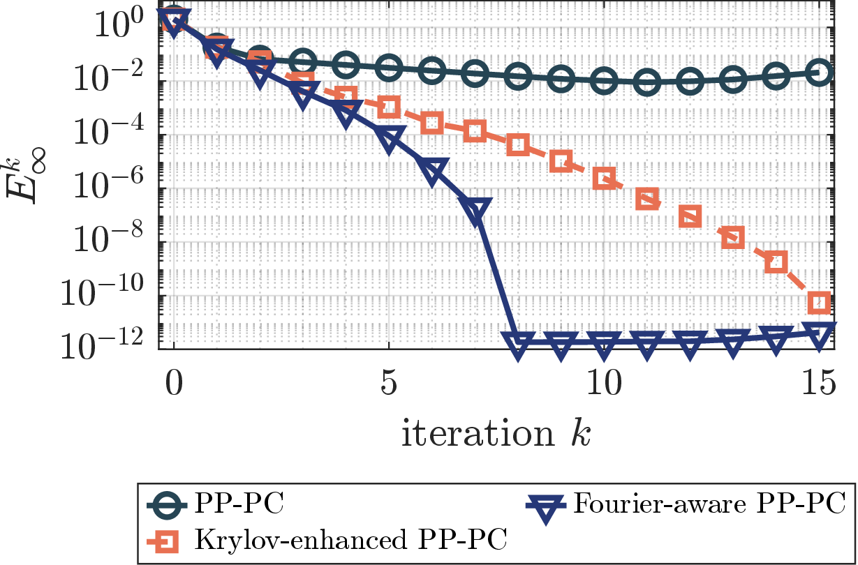
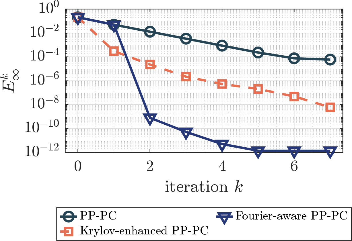
Figure 3: Error histories \(E_\infty^k\) of PP-PC, Krylov-enhanced PP-PC, and Fourier-aware PP-PC for the wave problem 27 (left, shown through \(k=15\)) and the forced Schrödinger problem 28 (right, shown through \(k=7\))..
| Problem | Method | \(E_\infty^{K}\) | \(E_\infty^k\le10^{-10}\) | \(\max_k\dim\) | \(|\mathcal I^k|\) |
|---|---|---|---|---|---|
| Wave \((K=8)\) | PP-PC | 1.5e-02 | – | 0 | – |
| Krylov-enhanced PP-PC | 4.2e-05 | – | 16 | – | |
| Fourier-aware PP-PC | 1.8e-12 | 8 | 32 | 3 | |
| Schrödinger \((K=16)\) | PP-PC | 4.4e-04 | – | 0 | – |
| Krylov-enhanced PP-PC | 1.0e-13 | 8 | 32 | – | |
| Fourier-aware PP-PC | 1.4e-12 | 3 | 30 | \(\le\)10 |
5.1.0.2 Evaluation of the tail–leak estimate
We evaluate 2 along the Fourier-aware iterations. For its cyclic factor \(\Gamma_k=\left\lVert \widehat{\mathcal{C}}_{P_{\mathcal{I}^k}}^{-1} \right\rVert_{\infty\to\infty}\), we use the computable block-row majorant \[\label{eq:block-row-majorant} \Gamma_k\le\overline{\Gamma}_k:=\max_{0\le n<N}\sum_{m=0}^{N-1} \left\lVert \bigl(\widehat{\mathcal{C}}_{P_{\mathcal{I}^k}}^{-1}\bigr)_{nm} \right\rVert_2.\tag{29}\] At the fixed discretization, the affine discrepancy has uniform Lipschitz constant \(\delta_{FG}:=\max_n\left\lVert F_n-G_n \right\rVert_2\), where \(F_n\) and \(G_n\) are the linear parts of \(\mathcal{F}_n\) and \(\mathcal{G}_n\). Applying the estimate with these computable quantities gives \[\label{eq:numerics-evaluated-bound} B_{k+1} := \overline{\Gamma}_k\,\delta_{FG}\, \frac{\operatorname{Tail}_{\mathcal{I}^k}\left(\mathbf{e}^k\right) +\operatorname{Leak}_{\mathcal{I}^k}^{P_{\mathcal{I}^k}}\left(\mathbf{e}^k\right)}{\sqrt N}.\tag{30}\] Thus \(E_\infty^{k+1}\le B_{k+1}\) in exact arithmetic. The tail and leak use the measured error history \(\mathbf{e}^k\), so \(B_{k+1}\) is a posteriori. The estimate therefore applies to the Crank–Nicolson wave propagator without a fine-propagator contraction assumption.
| Fourier-aware | Krylov-enhanced | ||||||
|---|---|---|---|---|---|---|---|
| 3-6(lr)7-8 Problem | \(k\) | \(\Tail\) | \(\Leak\) | \(B_{k+1}\) | \(E_\infty^{k+1}\) | \(\Tail\) | \(\Leak\) |
| Wave | 0 | 4.4e-13 | 3.8e-01 | 4.9e+02 | 1.5e-01 | 0 | 8.0e-01 |
| 2 | 5.0e-13 | 3.2e-03 | 7.0e+01 | 4.1e-03 | 0 | 1.6e-02 | |
| 4 | 1.1e-12 | 2.7e-05 | 1.6e+00 | 9.0e-05 | 0 | 1.2e-03 | |
| 6 | 9.0e-12 | 2.5e-08 | 1.1e-03 | 1.8e-07 | 0 | 8.6e-05 | |
| 7 | 8.5e-12 | 7.5e-12 | 4.4e-07 | 1.8e-12 | 0 | 2.1e-05 | |
| Schrödinger | 0 | 2.3e+00 | 0 | 1.1e+01 | 5.0e-02 | 0 | 2.8e-03 |
| 1 | 2.0e-13 | 7.8e-09 | 3.7e-07 | 7.9e-10 | 0 | 2.3e-04 | |
| 2 | 1.6e-13 | 4.5e-10 | 2.1e-08 | 5.2e-11 | 0 | 2.3e-05 | |
| 3 | 1.6e-13 | 3.6e-11 | 1.7e-09 | 5.0e-12 | 0 | 5.3e-06 | |
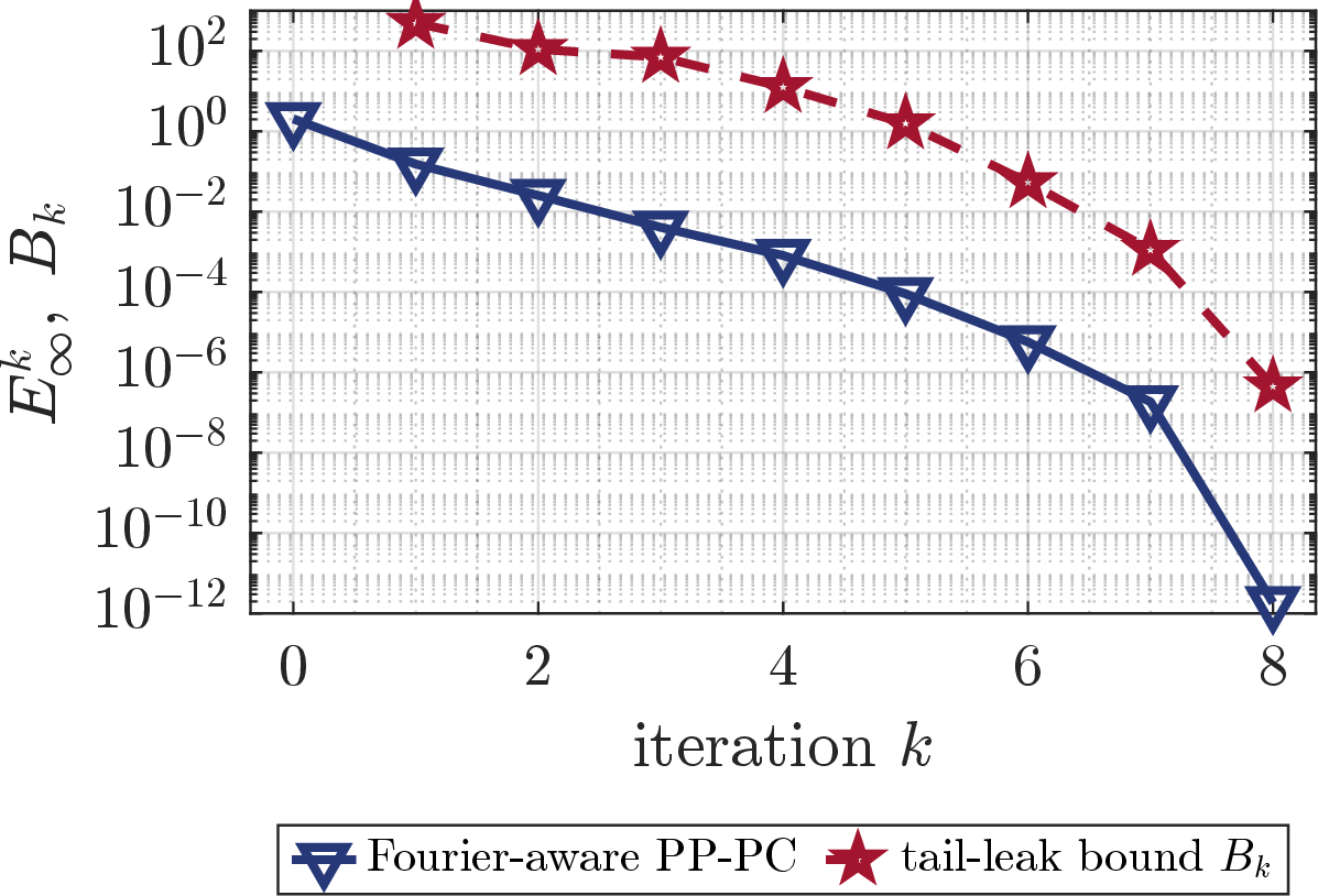
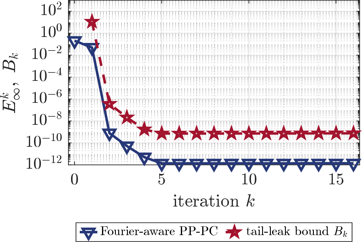
Figure 4: Measured error \(E_\infty^k\) of the Fourier-aware iterations and the evaluated tail–leak bound \(B_k\) of 30 for the wave (left) and Schrödinger (right) problems; \(B_0\) is not defined..
[tab:linear-tail-leak,fig:linear-bound] show that \(B_k\) lies above \(E_\infty^k\) at every computed step and follows the initial error decay. The bound is not sharp, remaining roughly two to five orders above the measured error. The prefactor \(\overline{\Gamma}_k\delta_{FG}\) contributes to this slack. The block-row majorant \(\overline{\Gamma}_k\) ranges over \(8\times10^1\)–\(4\times10^3\) for the wave problem and \(3\times10^1\)–\(3\times10^2\) for the Schrödinger problem, while \(\delta_{FG}\approx63\) and \(1.2\), respectively. The larger wave values of \(\overline{\Gamma}_k\) are consistent with its near-resonant discretization.
The tail and leak columns separate the two contributions to the unresolved-error bound. For the fixed-band wave problem, the Fourier-aware tail stays at roundoff level and the leak decays. For the adaptive Schrödinger problem, \(\mathcal{I}^0\) is empty, so all initial error modes contribute to the tail. After the first selection, the tail falls to roundoff level and the leak decays. For comparison, the table also reports Krylov-enhanced diagnostics in the all-mode representation of 1; its diagnostic tail is zero, but its leak need not be. Thus a small tail alone does not make the tail–leak bound small.
5.1.0.3 A posteriori test of projection dependence
For a fixed \(P\), 1 identifies two projection-dependent quantities in the next-step error bound: the unresolved-error norm \(\max_{0\le n<N}\left\lVert Q\mathbf{e}_n^k \right\rVert_2\), with \(Q=I-P\), and the cyclic stability factor \(\Gamma\) associated with \(\widehat{\mathcal{C}}_P\). To examine these quantities a posteriori, we use two frozen projection spaces. We construct \(P_F\) from the mixed Fourier space and \(P_K\) from the solution-snapshot space, using their respective histories through the same iteration \(k_\ast\). For each problem, \(k_\ast\) is the first iteration at which Fourier-aware PP-PC satisfies \(E_\infty^{k_\ast}\le10^{-10}\). We restart the same discrepancy-form update 3 from \(\mathbf{U}^0\) with each projection fixed, so only \(P\) differs. 3 reports \(\max_n\left\lVert Q\mathbf{e}_n^0 \right\rVert_2\), the corresponding block-row majorant \(\overline{\Gamma}(P)\) obtained from 29 , and \(E_\infty^1\); 5 shows the subsequent fixed-projection histories.
| Problem | Projection | \(\max_n\norm{Q\mathbf e_n^0}_2\) | \(\overline\Gamma(P)\) | \(E_\infty^1\) |
|---|---|---|---|---|
| Wave | \(P_F\) | 1.8e-12 | 1.76e+03 | 1.8e-12 |
| \(P_K\) | 6.7e-07 | 2.41e+03 | 1.0e-05 | |
| Schrödinger | \(P_F\) | 2.8e-12 | 3.08e+02 | 4.4e-12 |
| \(P_K\) | 4.7e-07 | 3.08e+02 | 5.3e-07 |
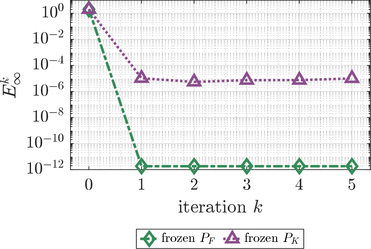
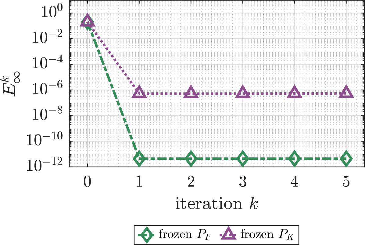
Figure 5: Error histories over five iterations after restarting projection-based PP-PC from \(\mathbf{U}^0\) with the discrepancy-form propagator and frozen projections \(P_F\) (mixed Fourier) and \(P_K\) (solution-snapshot) for the wave (left) and Schrödinger (right) problems..
Within each problem, the computed cyclic majorants are comparable, whereas the unresolved initial error for \(P_F\) is more than five orders of magnitude smaller than for \(P_K\). Consistently, \(P_F\) produces one-step errors of order \(10^{-12}\), while \(P_K\) produces errors of order \(10^{-5}\) and \(10^{-7}\) for the wave and Schrödinger problems, respectively. The subsequent fixed-projection histories preserve this separation. Within the evaluated estimate, the unresolved factor therefore provides the dominant separation between the two projections. Thus, in these tests, the reported Fourier-aware construction yields a more refined projection space for the error-relevant components.
5.2 Nonlinear problems↩︎
Both nonlinear problems have period \(T=1\) and periodic boundary conditions on \([0,1)\). We use second-order centered differences on \(32\) grid points (\(d=64\)), \(N=16\), and \(K=8\). The fine propagator is classical fourth-order Runge–Kutta with \(\delta t=1/512\). Writing the semi-discrete system as \(\mathbf{w}'=A\mathbf{w}+\mathbf{g}(\mathbf{w},t)\), the coarse propagator is an implicit–explicit (IMEX) Euler step [29], [30] \[\label{eq:numerics-semi-implicit} \mathcal{G}_n(\mathbf{w}) = \left(I-\Delta T\,A\right)^{-1} \left(\mathbf{w}+\Delta T\,\mathbf{g}(\mathbf{w},T_{n+1})\right), \qquad \Delta T=1/16.\tag{31}\] Thus the stiff linear part is implicit and the nonlinear part explicit, with one fixed-matrix solve per coarse step.
The first problem is the periodically forced Stuart–Landau reaction–diffusion system [31]. For \(w=p+\imath q\), \[\label{eq:numerics-stuart-landau} \begin{align} \partial_t w &= D\,\partial_{xx}w+(\lambda+\imath\omega)w -(1+\imath\beta)|w|^2w+f(x,t),\\ f(x,t) &= 0.5\left(\sin2\pi x+0.35\sin4\pi x\right)\cos2\pi t, \end{align}\tag{32}\] where \(D=0.05\), \(\lambda=0.5\), \(\omega=2\pi\), and \(\beta=1\).
The second problem is the periodically forced Brusselator [32], with \(a=1\), \(b=3\), \(D_1=10^{-2}\), \(D_2=5\times10^{-3}\), and the same forcing \(f\): \[\label{eq:numerics-brusselator} \begin{align} \partial_t u &= D_1\,\partial_{xx}u+a-(b+1)u+u^2v+f(x,t),\\ \partial_t v &= D_2\,\partial_{xx}v+bu-u^2v. \end{align}\tag{33}\] Although the forcing contains only the temporal frequency \(\ell=1\), the nonlinear terms generate higher harmonics. Both tests therefore use the fixed 7-mode band \(\mathcal{I}_3=\{0,1,2,3,N-3,N-2,N-1\}\).
The two problems exercise the two stability mechanisms evaluated below. For Stuart–Landau, the measured linearization of \(\mathcal{H}_{P^k,n}\) along the fine reference is contractive, so its evaluated bound uses the loop-gain specialization associated with 5. For the Brusselator, the corresponding linearization is noncontractive, so its evaluated bound uses the general cyclic-inverse form. The local nondegeneracy condition of 3 and the smallness condition ?? are examined below. The cyclic-inverse analysis therefore covers noncontractive settings in which the linearized cyclic operator remains invertible, beyond the contraction-based stability mechanism used in earlier quantitative nonlinear PP-PC estimates [19].
5.2.0.1 Convergence comparison
[fig:nonlinear-convergence,tab:nonlinear-summary] show that Fourier-aware PP-PC reaches \(E_\infty^k\le10^{-10}\) first, at \(k=2\) for Stuart–Landau and \(k=4\) for the Brusselator, and is the only method to do so in both tests within \(K=8\). Under the same rank-revealing procedure, its maximal projection-space dimension is smaller than that of Krylov-enhanced PP-PC in both tests. The panels show the histories through \(k=6\), while the table summarizes the complete \(K=8\) runs by their final errors, threshold iterations, maximal dimensions, and mode counts.
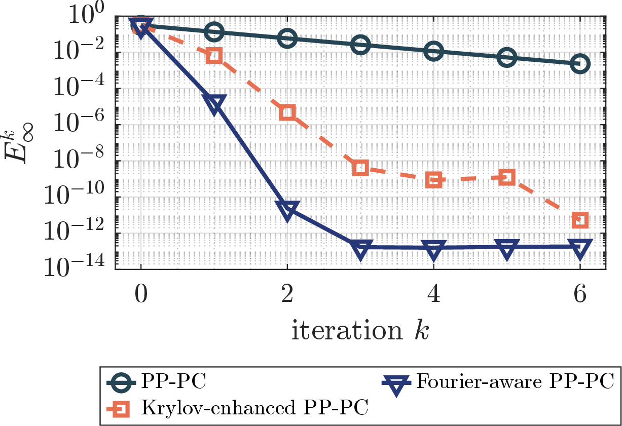
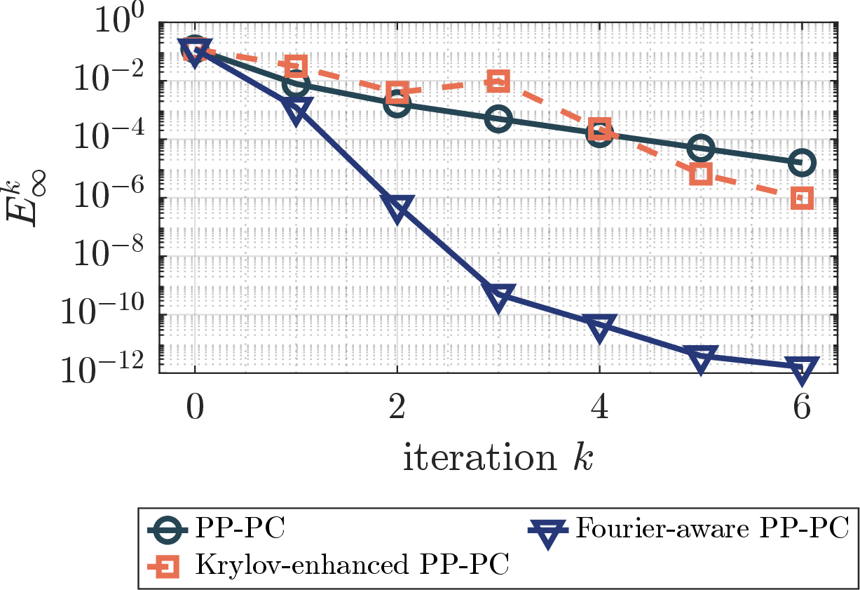
Figure 6: Error histories \(E_\infty^k\) of PP-PC, Krylov-enhanced PP-PC, and Fourier-aware PP-PC for the forced Stuart–Landau problem 32 (left) and the forced Brusselator problem 33 (right), shown through \(k=6\)..
| Problem | Method | \(E_\infty^{K}\) | \(E_\infty^k\le10^{-10}\) | \(\max_k\dim\) | \(|\mathcal I^k|\) |
|---|---|---|---|---|---|
| Stuart–Landau \((K=8)\) | PP-PC | 4.5e-04 | – | 0 | – |
| Krylov-enhanced PP-PC | 6.2e-13 | 6 | 23 | – | |
| Fourier-aware PP-PC | 1.8e-13 | 2 | 17 | 7 | |
| Brusselator \((K=8)\) | PP-PC | 1.7e-06 | – | 0 | – |
| Krylov-enhanced PP-PC | 4.1e-09 | – | 51 | – | |
| Fourier-aware PP-PC | 2.9e-13 | 4 | 36 | 7 |
5.2.0.2 Projection-level decomposition of the local one-step factor
For \(P=P_{\mathcal{I}^k}\), set \(Q=I-P_{\mathcal{I}^k}\) and define \(m_Q^k:=\max_{0\le n<N}\left\lVert Q\mathbf{e}_n^k \right\rVert_2\) and \(m_P^k:=\max_{0\le n<N}\left\lVert P_{\mathcal{I}^k}\mathbf{e}_n^k \right\rVert_2\); abbreviate \(U_k^\perp:=U_k^\perp(P_{\mathcal{I}^k})\). For the Fourier-aware projection, these definitions and 2 give \[\begin{align} m_Q^k &=E_\infty^k\theta_Q^k(P_{\mathcal{I}^k}) \le \widetilde{m}_Q^k :=\frac{\operatorname{Tail}_{\mathcal{I}^k}(\mathbf{e}^k) +\operatorname{Leak}_{\mathcal{I}^k}^{P_{\mathcal{I}^k}}(\mathbf{e}^k)}{\sqrt N} =E_\infty^k\Theta_Q^k,\\ m_P^k&=E_\infty^k\Theta_P^k. \end{align}\] Thus, after multiplication by \(E_\infty^k\), the factor in 1 has the three numerator contributions \[\mu_k\,m_Q^k, \qquad \nu_k\,U_k^\perp m_P^k, \qquad \frac{\nu_k}{2}m_Q^k m_P^k.\] 5 reports this majorant, the three unweighted factors, and the resulting \(E_\infty^{k+1}\).
In both problems, \(m_Q^k\) is the largest unweighted factor. The measured weights preserve this dominance. The discrepancy-curvature factor \(m_Q^km_P^k\) is smaller and quadratic in the error, while \(U_k^\perp m_P^k\) is negligible. Over the reported steps, \(\Theta_Q^k=\widetilde{m}_Q^k/E_\infty^k\le4.93\times10^{-2}\), so the normalized tail–leak sum is small. Since \(\widetilde{m}_Q^k\) majorizes the dominant unresolved factor, these data provide a posteriori evidence that a small tail together with a small leak is associated with the observed rapid next-step decay; the complete estimate is evaluated below.
5.2.0.3 Evaluation of the nonlinear tail–leak estimate
Thus 1 replaces \(m_Q^k\) by its tail–leak majorant \(\widetilde{m}_Q^k\) in the unresolved-error and discrepancy-curvature contributions, while leaving the base-state contribution unchanged.
| Problem | \(k\) | \(E_\infty^k\) | \(\widetilde m_Q^k\) | \(m_Q^k\) | \(U_k^\perp m_P^k\) | \(m_Q^k m_P^k\) | \(E_\infty^{k+1}\) |
|---|---|---|---|---|---|---|---|
| Stuart–Landau | 0 | 3.1e-01 | 6.8e-05 | 6.7e-05 | 4.9e-11 | 2.1e-05 | 1.8e-05 |
| 1 | 1.8e-05 | 6.2e-10 | 1.6e-10 | 7.5e-17 | 2.8e-15 | 2.4e-11 | |
| 2 | 2.4e-11 | 1.2e-12 | 9.4e-13 | 2.1e-23 | 2.2e-23 | 1.7e-13 | |
| Brusselator | 0 | 1.2e-01 | 3.5e-03 | 3.4e-03 | 1.2e-09 | 4.2e-04 | 1.2e-03 |
| 1 | 1.2e-03 | 1.5e-06 | 1.4e-06 | 7.0e-12 | 1.8e-09 | 5.4e-07 | |
| 2 | 5.4e-07 | 2.2e-09 | 2.0e-09 | 2.7e-17 | 1.1e-15 | 4.9e-10 |
The corresponding diagnostic weighted sum is \[\mathcal{S}_{k,\mathrm F} :=\hat{\mu}\,\widetilde{m}_Q^k +\hat{\nu}\,U_k^\perp m_P^k +\frac{\hat{\nu}}{2}\widetilde{m}_Q^k m_P^k.\]
For Stuart–Landau, the computed finite-difference (FD) reference-Jacobian norm \[\hat{\alpha}_k :=\max_n\left\lVert J_{\mathcal{H}_{P_{\mathcal{I}^k},n}}^{\rm FD} (\mathbf{u}_n^\star) \right\rVert_2 \approx0.956<1,\] giving the loop-gain specialization \[\label{eq:numerics-estimated-nl-bound} B_{k+1,\mathrm F}^{\mathrm{nl}} :=\frac{\mathcal{S}_{k,\mathrm F}}{(1-\hat{\alpha}_k)-\tfrac12\hat{\kappa}_kR}.\tag{34}\] For the Brusselator, whose reference linearization is noncontractive, we use the general cyclic-inverse form \[\label{eq:numerics-nk-nl-bound} B_{k+1,\mathrm F}^{\mathrm{nl}} :=\frac{\overline{\widehat\Gamma}_k}{1-\tfrac12\overline{\widehat\Gamma}_k\hat{\kappa}_kR} \mathcal{S}_{k,\mathrm F}.\tag{35}\]
Here \(\overline{\widehat\Gamma}_k\) is defined analogously by the block-row formula in 29 , using the assembled finite-difference cyclic matrix. With exact Jacobians, the same construction majorizes \(\widehat\Gamma_k=\left\lVert \widehat{\mathcal{C}}_{P_{\mathcal{I}^k}}^{-1} \right\rVert_{\infty\to\infty}\); the prefactor is increasing in this norm while its denominator is positive, so the majorization preserves the exact bound.
We take \(R=E_\infty^0\). The Stuart–Landau denominator is positive, while for the Brusselator \(\overline{\widehat\Gamma}_k\in[62,66]\) and \(\tfrac12\overline{\widehat\Gamma}_k\hat{\kappa}_kR \in[0.50,0.66]\); moreover, \(E_\infty^{k+1}\le R\) holds throughout both runs. All diagnostic Jacobians use central differences with step \(10^{-6}(1+\left\lVert \mathbf{x} \right\rVert_\infty)\). Those at \(\mathbf{u}^\star\) give \(\hat{\alpha}_k\) and the cyclic matrix used to form \(\overline{\widehat\Gamma}_k\), while \(\hat{\mu}\) maximizes discrepancy-Jacobian norms at \(\mathbf{u}^\star\) and \(\mathbf{U}^0\). The estimate \(\hat{\nu}\) uses Jacobian difference quotients between these two histories and along two directions generated with seed \(0\) and scaled to radius \(E_\infty^0\) at each time point; the same directional sampling of the Jacobians of \(\mathcal{H}_{P_{\mathcal{I}^k},n}\) gives the sampled curvature \(\hat{\kappa}_k\). These finite-difference and sampled quantities are diagnostic estimates rather than certified bounds for the exact local constants.
7 shows that both evaluated estimates lie above the realized errors and follow their decay. Relative to the projection-level estimate, the tail–leak majorization adds, over the evaluated iterations, at most factors \(3.97\) and \(1.45\) for Stuart–Landau and the Brusselator, respectively. Thus 5 isolates the local projection mechanism, while 7 evaluates the corresponding Fourier tail–leak estimate of 1, including the noncontractive regime.
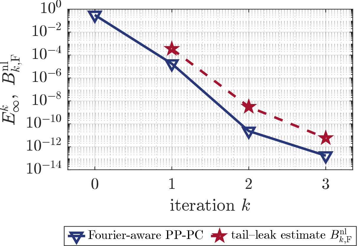
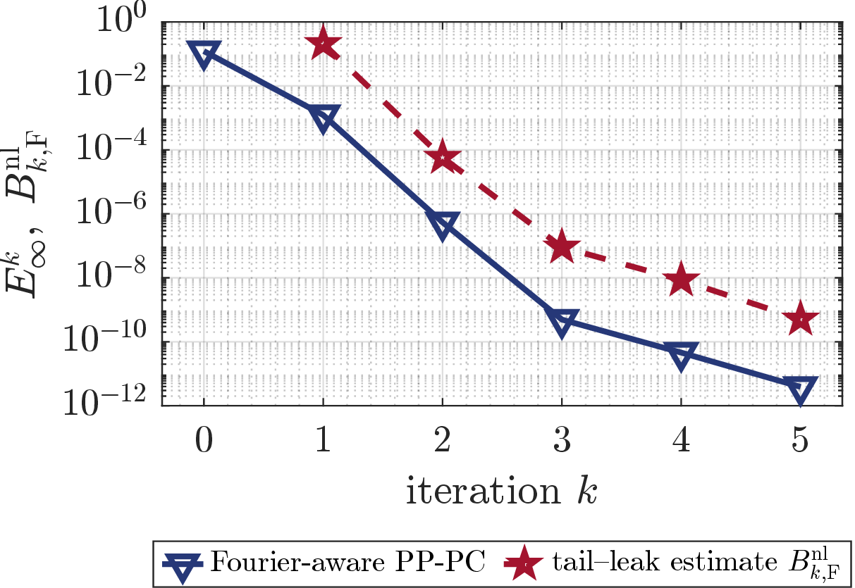
Figure 7: Measured errors \(E_\infty^k\) and evaluated nonlinear tail–leak estimates \(B_{k,\mathrm F}^{\mathrm{nl}}\) of 1. Left: the loop-gain specialization 34 for Stuart–Landau. Right: the cyclic-inverse form 35 for the Brusselator. The value \(B_{0,\mathrm F}^{\mathrm{nl}}\) is not defined..
5.3 Summary and discussion↩︎
[tab:linear-summary,tab:nonlinear-summary] show that Fourier-aware PP-PC reaches \(E_\infty^k\le10^{-10}\) in the fewest outer iterations in all four examples. Its maximal projection-space dimension is smaller than that of Krylov-enhanced PP-PC in three examples. For the wave problem it is larger, but the tolerance is reached at \(k=8\) rather than \(k=15\) (3). The frozen-projection experiment illustrates the dependence on \(P\) in 1: at the same history depth, the mixed Fourier spaces leave smaller unresolved errors and produce smaller one-step errors under comparable computed cyclic majorants (3 5).
For the linear problems, the measured tail–leak quantities and evaluated bound are consistent with 2 (2 4). For the nonlinear problems, 5 identifies \(m_Q^k\) as the largest unweighted projection-level factor. Over the reported steps, \(\Theta_Q^k\le4.93\times10^{-2}\). 7 evaluates the nonlinear tail–leak estimate using diagnostic estimates of the local constants for the Stuart–Landau and Brusselator cases, whose computed finite-difference reference linearizations are contractive and noncontractive, respectively. Taken together, these results indicate that the mixed Fourier construction yields a more refined projection space in the reported tests: it is better aligned with error-relevant directions but not always smaller.
6 Conclusion and future work↩︎
We introduced Fourier-aware projection-based PP-PC, a projection-based periodic parareal method that combines a discrepancy-based correction scheme with a Fourier-aware projection space. We developed a convergence analysis for general nonlinear time-periodic problems, in which a temporal tail–leak bound controls both the unresolved-error term and the nonlinear remainder in a local one-step estimate, and showed that the linear case reduces to global bounds under weaker assumptions. We demonstrated on linear and nonlinear problems that Fourier-aware PP-PC converges faster than Krylov-enhanced PP-PC, with the measured errors consistent with the analysis.
Our comparisons measure outer-iteration convergence, as in [19], [23]. Since the corrected periodic solve is more expensive per iteration than the coarse solve of the original PP-PC, a work-normalized timing study and dedicated fast solvers for it are subjects of further study.
Acknowledgments↩︎
This work was supported by the National Key R&D Program of China under Grant Nos. 2020YFA0711900 and 2020YFA0711902. During the preparation of this manuscript, the authors used OpenAI’s ChatGPT to improve its readability and assist with the design of code for the numerical experiments. The authors assume responsibility for all content.
References↩︎
School of Mathematical Sciences, Fudan University, Shanghai, China (, , , ).↩︎