SinCoTrap: A High-Order Locally Corrected Trapezoidal Rule for Periodic Singular Integrals in Arbitrary Dimensions
July 14, 2026
Abstract
We present SinCoTrap (Singularity-Corrected Trapezoidal Rule), a high-order locally corrected trapezoidal method for periodic singular integrals in arbitrary dimension \(d\) with kernel \(|\boldsymbol{x}|^{-s}\), \(0<s<d\). The scheme preserves the uniform tensor grid and modifies only a fixed, small stencil of weights near the singularity. For a correction order \(p\), the resulting quadrature attains the error rate \(O(h^{2p+2+d-s})\). We derive explicit, mesh-independent limiting correction weights via analytic continuation of a special generalization of the Riemann zeta function, yielding rapidly computable formulas that can be pretabulated for each \((d,s,p)\). This makes SinCoTrap both efficient in application and robust for high-order accuracy across a broad class of periodic singular integrals.
1 Introduction↩︎
Singular integrals frequently arise in numerical analysis and scientific computing in many applications. Accurate evaluation of these integrals is essential for reliable computation of physical quantities, but the presence of singularities poses significant challenges for standard quadrature methods. Specifically, we focus on singular integrals in arbitrary dimension \(d\) that takes the form \[I[\varphi\cdot \sigma] = \int_V \varphi(\boldsymbol{x}) \sigma(\boldsymbol{x}) \mathrm{d}\boldsymbol{x}, \quad \sigma(\boldsymbol{x}) = \frac{1}{|\boldsymbol{x}- \boldsymbol{x}_0|^{s}}, \quad \boldsymbol{x}\in \mathbb{R}^d,\] where \(\sigma(\boldsymbol{x})\) is a singular function with an isolated singularity at \(\boldsymbol{x}_0 \in \mathrm{Int}(V)\) for \(0 < s < d\), \(\varphi(\boldsymbol{x})\) is a smooth function, and the entire integrand \(\varphi(\boldsymbol{x})\sigma(\boldsymbol{x})\) is smooth except at the singular points and is periodic with unit cell \(V\). Equivalently, \(\varphi\cdot\sigma\) defines a \(C^{\infty}\) function on the punctured torus.
Various approaches have been developed for singular quadrature to address the challenges posed by singularities, which can be broadly classified into three categories: (1) Singularity cancellation [1], where a change of variables (such as to spherical coordinates) cancels the singularity via the Jacobian, allowing standard quadrature rules to be applied to the resulting regular integral; (2) Singularity subtraction [2], [3], where the singular component is subtracted from the integrand and integrated separately by introducing an auxiliary function that closely approximates the singular behavior, while the regular part is handled numerically; and (3) Singularity correction [4]–[6], where the quadrature weights are modified to account for the effect of the singularity and achieve high-order accuracy.
Our focus in this work is on the third category, specifically on singularity correction methods for trapezoidal rule. The trapezoidal rule is a simple, stable, and widely used quadrature method, celebrated for its super-algebraic convergence for smooth periodic functions [7]. Its accuracy deteriorates when either periodicity or smoothness is lost: a smooth non-periodic integrand creates boundary error, which can be corrected by endpoint or near-boundary modifications, whereas a periodic integrand with an isolated singularity, as in the present work, creates a local singularity error. In both cases, one modifies only a small number of quadrature weights while retaining the underlying uniform grid. The resulting correction weights can be precomputed for a given boundary behavior or singularity type and reused for a broad class of problems.
The pioneering corrected trapezoidal rule was introduced by Rokhlin [6] for one-dimensional endpoint singularities. The central concept of the method involves adding local correction terms to analytically cancel the leading-order terms of the quadrature error of the trapezoidal rule. The correction weights are computed by solving a linear system, constructed by requiring that the corrected rule integrate exactly over the monomials, up to a desired degree, multiplying the singular function. However, the practical utility of this approach is limited because achieving high-order accuracy requires correction weights whose magnitude grows rapidly, leading to numerical instability.
Subsequent work by Kapur and Rokhlin [4] extended this approach by introducing additional quadrature nodes outside the integration interval. This strategy yielded smaller correction weights and enabled higher-order accuracy. Furthermore, they derived a mesh-size-independent rule by computing the asymptotic limit of the weights as \(h\rightarrow 0\), enhancing its practical utility, though explicit closed-form expressions for these limiting weights were not provided. The principal drawbacks of this scheme are its requirement for function evaluations outside the domain, which can be problematic or undefined, and the difficulties involved in computing the asymptotic weights.
To address these issues, Marin et al. [5] introduced an alternative approach using a compactly supported smooth window function \(g(\boldsymbol{x})\). By multiplying the singular function by \(g(\boldsymbol{x})\), the singularity is localized and the effect of boundary errors are annihilated, thereby simplifying the computation of the correction weights. For one-dimensional singular kernels of the form \(\sigma(\boldsymbol{x})=|\boldsymbol{x}|^s\) with \(s > -1\), they derived an explicit formula for the converged weights, revealing a connection to the Riemann zeta function. The method was also extended to two dimensions for the singular kernel \(\sigma(\boldsymbol{x})=1/|\boldsymbol{x}|\), although a closed-form expression for the converged weights remained elusive. Later work by Jiang and Li [8] improved the two-dimensional scheme by proving the non-singularity of the underlying linear system for solving the correction weights and employing Richardson extrapolation to compute the weights numerically. Besides, Wu and Martinsson [9] found an implicit formula for the two-dimensional weights, connecting them to the higher-order parametric derivatives of the Epstein zeta function.
In this work, motivated by the need to accelerate the convergence of thermodynamic limit of exchange energy in electronic structure calculations [10], [11] without increasing computational cost, we extend the one dimensional high-order, singularity-corrected trapezoidal rules for singular functions in [5] to arbitrary dimensions. Our contributions are twofold. First, we provide a rigorous analysis of the corrected trapezoidal rule’s construction in a multi-dimensional setting. Second, we derive simple and explicit formulas for the correction weights via analytic continuation, which enable their efficient and accurate computation, thereby significantly enhancing the method’s practical utility.
Beyond exchange energy calculations in electronic structure theory, singularity corrected trapezoidal rules find broad applications across scientific and engineering disciplines. For example, the evaluation of surface singular integrals in boundary integral equations in 2D [12], [13] and 3D [9], [14], [15]; the numerical discretization of the fractional Laplacian in non-local Fokker-Planck equations in 2D [8]; the computation of Coulomb potentials in 3D [16]; and the evaluation of integral operators in Lippmann-Schwinger equations for scattering problems [17].
The rest of this paper is organized as follows. 2 details the algorithm for the singularity-corrected trapezoidal rule in arbitrary dimensions, including the explicit construction of the correction weights. 3 provides a theoretical analysis of the method’s convergence, establishing guarantees for its high-order accuracy. 4 discusses extensions of the method to parallelotope domains and anisotropic types of singularities. Numerical results in 5 validate the theoretical analysis and demonstrate the algorithm’s practical performance. Finally, 6 offers concluding remarks, while the Appendix collects supporting proofs and technical derivations.
2 Singularity corrected trapezoidal rule↩︎
This section presents a systematic framework for constructing a locally corrected trapezoidal rule that handles isolated singularities in arbitrary dimensions. We begin by establishing the necessary notation and motivating the design of the local correction procedure. Subsequently, we provide a complete description of the algorithm, including explicit constructions for the correction weights. For clarity, extended proofs and technical derivations are deferred to the appendix.
Setup and notations↩︎
In this paper, we denote integer lattice points with bold letters (e.g., \(\boldsymbol{i}\in\mathbb{Z}^d\)). Furthermore, we use Greek letters, such as \(\boldsymbol{\alpha}= (\alpha_1, \ldots, \alpha_d) \in \mathbb{N}^d\), to represent nonnegative integer lattice points, which frequently serve as multi-indices in Taylor expansions. The distinction between general integer points \(\boldsymbol{i}\) and nonnegative multi-indices \(\boldsymbol{\alpha}\) will be clear from context. For vector \(\boldsymbol{i}=(i_1,\ldots,i_d) \in \mathbb{R}^d\), different norms for vectors are defined as follows: \[| \boldsymbol{i} |_\infty := \max(|i_1|, \cdots, |i_d|), \quad | \boldsymbol{i} |_1 := |i_1| + \cdots + |i_d|, \quad |\boldsymbol{i}| := \left(|i_1|^2 + \cdots + |i_d|^2\right)^{1/2}.\]
By translation, we assume the isolated singularity is located at the origin and consider \[I[\varphi\cdot \sigma] = \int_V \varphi(\boldsymbol{x})\sigma(\boldsymbol{x})\,\mathrm{d}\boldsymbol{x}, \qquad \sigma(\boldsymbol{x}) = \frac{1}{|\boldsymbol{x}|^{s}}, \qquad 0 < s < d,\] where \(\varphi\) is smooth, \(\varphi\cdot\sigma\) is smooth except at the singular points and periodic with unit cell \(V=[-a,a]^d\) for some \(a>0\).
We discretize \(V\) by a uniform tensor-product grid. Let \(N\in\mathbb{N}_{+}\) and set mesh size \(h=a/N\). For lattice indices \(\boldsymbol{i}=(i_1,\ldots,i_d)\in\mathbb{Z}^d\), define grid points \[\boldsymbol{x}_{\boldsymbol{i}} := \boldsymbol{i}h, \qquad \mathcal{X}:= \{\boldsymbol{x}_{\boldsymbol{i}} : | \boldsymbol{i} |_\infty\le N\}.\] The set \(\mathcal{X}\) contains the origin and is symmetric in the sense that \(\boldsymbol{x}_{\boldsymbol{i}}\in\mathcal{X}\) implies \(-\boldsymbol{x}_{\boldsymbol{i}}\in\mathcal{X}\).
Finally, we denote by \(T_h^0[f]\) the punctured trapezoidal rule (excluding the origin). It is convenient to write it in the tensor-product form 3 \[T_h^0[f] := h^d \sum_{0 < | \boldsymbol{i} |_\infty \leq N} c_{\boldsymbol{i}}\, f(\boldsymbol{x}_{\boldsymbol{i}}), \qquad c_{\boldsymbol{i}} := 2^{-m(\boldsymbol{i})}, \quad m(\boldsymbol{i}):=\#\{j: |i_j|=N\}.\] Thus \(c_{\boldsymbol{i}}=1\) for interior points, and each boundary coordinate contributes a factor \(1/2\) (e.g., in three dimensions: face/edge/corner weights \(1/2\), \(1/4\), \(1/8\)).
2.1 Motivation↩︎
For smooth periodic integrands, the trapezoidal rule converges super-algebraically [7]. However, in our setting, the integrand satisfies smooth periodic boundary condition but has an isolated singularity at the origin, which limits the convergence of the standard rule. The goal of singularity correction is to restore high-order accuracy by modifying only a small number of quadrature weights near the singular point.
2.1.0.1 Step 1: extract the singularity effect.
Note that the boundary coordinates in the trapezoidal rule involve more complicated weights, in order to simplify the analysis and focus on the singularity, we introduce a smooth radial cutoff function \[\label{eq:boundary95cutoff} \eta(\boldsymbol{x}) = \eta(|\boldsymbol{x}|) = \begin{cases} 1, & |\boldsymbol{x}|\leq \frac{a}{4},\\ 0, & |\boldsymbol{x}|\geq \frac{a}{2}. \end{cases}\tag{1}\] This cutoff separates the local singularity effect and the boundary contribution, which makes the singular correction independent of the particular quadrature treatment [4], [18] used near the boundary for more general boundary conditions.
Using the cutoff function \(\eta(\boldsymbol{x})\), we split: \[I[\varphi\cdot\sigma] = \int_V \varphi(\boldsymbol{x})\sigma(\boldsymbol{x})\left(1-\eta(\boldsymbol{x})\right)\mathrm{d}\boldsymbol{x} + \int_V \varphi(\boldsymbol{x})\sigma(\boldsymbol{x})\,\eta(\boldsymbol{x})\mathrm{d}\boldsymbol{x}.\] The first integrand agrees with the original integrand near \(\partial V\) and is smooth periodic; hence its trapezoidal error is super-algebraically small. The second term is supported strictly inside \(V\) and contains the singularity at the origin. Therefore, by introducing \(\phi=\varphi\eta\), it suffices to focus on integrals of the form \[I[\phi\cdot\sigma] = \int_V \phi(\boldsymbol{x})\sigma(\boldsymbol{x})\,\mathrm{d}\boldsymbol{x},\] where \(\phi\) is smooth and compactly supported in \(V\).
2.1.0.2 Step 2: local Taylor surrogate and the correction term.
The difficulty is that \(\phi(\boldsymbol{x})\sigma(\boldsymbol{x})\) is singular at \(\boldsymbol{x}=0\). To isolate the leading singular behavior and improve the smoothness of the integrand, fix an order \(p\in\mathbb{N}\) and introduce a localized Taylor surrogate. Let \(P_{\phi}\) be the Taylor polynomial of \(\phi\) at \(\boldsymbol{x}=0\) of degree \(2p+1\), \[P_{\phi}(\boldsymbol{x}) := \sum_{| \boldsymbol{\alpha} |_1=0}^{2p+1} \frac{\partial^{\boldsymbol{\alpha}}\phi(0)}{\boldsymbol{\alpha}!}\,\boldsymbol{x}^{\boldsymbol{\alpha}},\] and choose a radial localized window function \(g\in C_c^{\infty}(V)\) such that \[\label{eq:localized95function95g} g(\boldsymbol{x})=g(|\boldsymbol{x}|),\qquad g(0)=1,\qquad \partial^{\boldsymbol{\alpha}}g(0)=0, \quad 1\leq | \boldsymbol{\alpha} |_1\leq 2p+1.\tag{2}\] Define \(\tilde{\phi}(\boldsymbol{x}):=P_{\phi}(\boldsymbol{x})g(\boldsymbol{x})\). Then \(\phi-\tilde{\phi}\) is compactly supported in \(V\) and vanishes to order \(2p+1\) at the origin: \[\partial^{\boldsymbol{\alpha}}\bigl(\phi-\tilde{\phi}\bigr)(0)=0, \quad 0\leq | \boldsymbol{\alpha} |_1\leq 2p+1,\] so that \((\phi-\tilde{\phi})(\boldsymbol{x})=O(|\boldsymbol{x}|^{2p+2})\) near the origin. Hence \((\phi-\tilde{\phi})(\boldsymbol{x})\sigma(\boldsymbol{x})=O(|\boldsymbol{x}|^{2p+2-s})\), which has a weakened singularity compared with \(\phi(\boldsymbol{x})\sigma(\boldsymbol{x})\). This suggests the decomposition \[\begin{align} I[\phi\cdot\sigma] &= I[(\phi-\tilde{\phi})\cdot\sigma] + I[\tilde{\phi}\cdot\sigma] \\ &= T_h^0[\phi\cdot\sigma] + (I-T_h^0)[(\phi-\tilde{\phi})\cdot\sigma] + \bigl(I[\tilde{\phi}\cdot\sigma]-T_h^0[\tilde{\phi}\cdot\sigma]\bigr). \end{align}\] The remaining task is to approximate the last difference \(I[\tilde{\phi}\cdot\sigma]-T_h^0[\tilde{\phi}\cdot\sigma]\) by a local correction supported on a fixed stencil near \(\boldsymbol{x}=0\).
2.1.0.3 Step 3: moment matching and a linear system.
Motivated by Step 2, we approximate the local defect \(I[\tilde{\phi}\cdot\sigma]-T_h^0[\tilde{\phi}\cdot\sigma]\) by a correction supported on a small stencil \(\mathcal{X}_p\subset\mathbb{Z}^d\): \[I[\tilde{\phi}\cdot \sigma] - T_h^0[\tilde{\phi}\cdot \sigma] = a(h) \sum_{\boldsymbol{i}\in \mathcal{X}_p} w_{\boldsymbol{i}}^h \, \tilde{\phi}(\boldsymbol{i}h),\] where \(a(h)\) is a scaling factor and \(\{w_{\boldsymbol{i}}^h\}\) are correction weights. Since \(\tilde{\phi}=P_\phi g\), this requirement is enforced by matching the trapezoidal defect on localized monomials. That is, for all multi-indices \(\boldsymbol{\alpha}\) with \(0\le | \boldsymbol{\alpha} |_1\le 2p+1\), we impose \[\label{eq:weight95equation} \int_V g(\boldsymbol{x})\sigma(\boldsymbol{x})\boldsymbol{x}^{\boldsymbol{\alpha}}\,\mathrm{d}\boldsymbol{x} = T_h^0[g\cdot\sigma\cdot \boldsymbol{x}^{\boldsymbol{\alpha}}] + a(h) \sum_{\boldsymbol{i}\in\mathcal{X}_p} w_{\boldsymbol{i}}^h\,(\boldsymbol{i}h)^{\boldsymbol{\alpha}}\,g(\boldsymbol{i}h).\tag{3}\] This gives a finite linear system for the unknowns \(\{w_{\boldsymbol{i}}^h\}\). Because \(g(\boldsymbol{x})\) and \(\sigma(\boldsymbol{x})\) are radial, and because the domain, grid, and stencil are symmetric, the moment conditions associated with odd monomials are automatically satisfied. Thus the system reduces to even moments and can be made square by a suitable choice of \(\mathcal{X}_p\), together with symmetry conditions on the weights.
In practice we will avoid constructing \(P_\phi g\) or evaluating derivatives of \(\phi\). Thus, the resulting corrected trapezoidal rule is defined by applying the same local correction to the original function \(\phi\): \[T_h^0[\phi\cdot\sigma] + a(h)\sum_{\boldsymbol{i}\in\mathcal{X}_p} w_{\boldsymbol{i}}^h\,\phi(\boldsymbol{i}h).\]
Finally, letting \(h\to 0\) yields converged weights \(w_{\boldsymbol{i}}=\lim_{h\to 0^+} w_{\boldsymbol{i}}^h\) that are independent of \(h\) (and, in fact, independent of the particular choice of \(g\) within the above class). We highlight that these converged weights give the same approximation order as the \(h\)-dependent weights, while being more practical to compute and apply.
2.2 Linear system for the correction weights↩︎
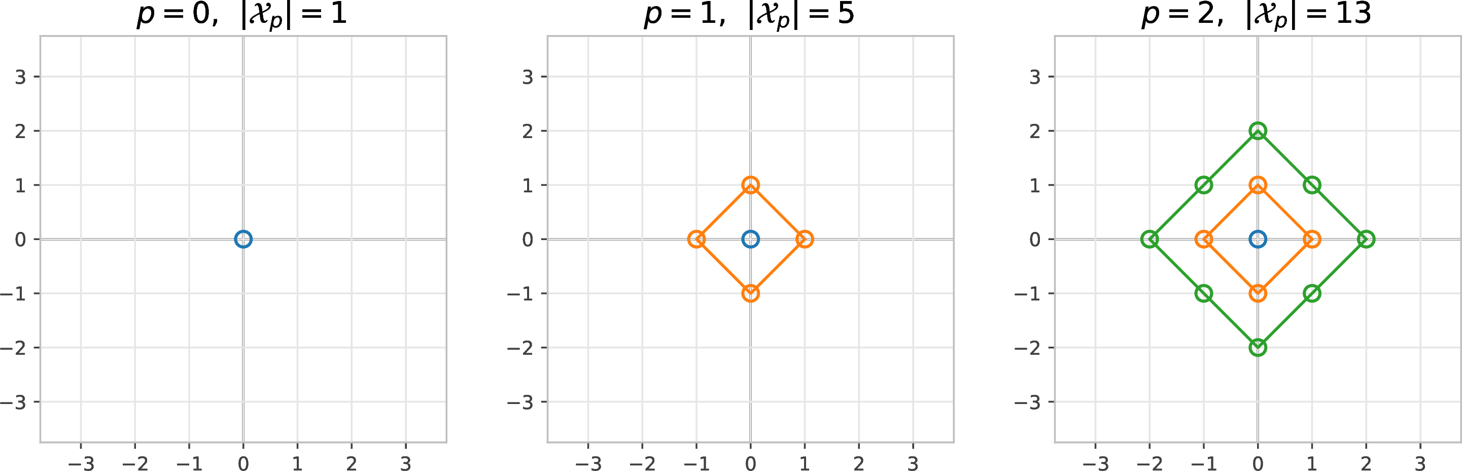
We now derive the concrete linear system for the correction weights. In this paper, we adopt the correction stencil \(\mathcal{X}_p\) with \(p \in \mathbb{N}\) defined as \[\mathcal{X}_p = \left\{ \boldsymbol{i}\in \mathbb{Z}^d \, : \, 0 \leq | \boldsymbol{i} |_1 \leq p \right\}.\] This is a natural choice for the radial singular kernel \(1/|\boldsymbol{x}|^s\), though other stencils are possible. For illustration, we visualize these stencils for \(d=2\) and \(p=0, 1, 2\) in 1.
Given the radial symmetry of both the singular kernel and the localized function \(g(\boldsymbol{x})\), and the symmetry of the integral domain \(V\) and grid points \(\mathcal{X}\), we enforce symmetry of the weights under independent sign flips of each coordinate. For \(\boldsymbol{\beta}=(\beta_1, \beta_2, \ldots, \beta_d) \in\mathbb{N}^d\), define the sign-orbit \[\mathcal{G}_{\boldsymbol{\beta}} := \left\{ (\pm \beta_1, \pm \beta_2, \ldots, \pm \beta_d) \in \mathbb{Z}^d \right\}.\] We then impose the symmetry constraint \[\label{eq:symmetric95condition} w_{\boldsymbol{i}}^h = w_{\boldsymbol{\beta}}^h, \quad \text{for } \boldsymbol{i}\in \mathcal{G}_{\boldsymbol{\beta}}, \, \, 0 \leq | \boldsymbol{\beta} |_1 \leq p.\tag{4}\] Under the symmetry of weights, all moment constraints in 3 associated with odd monomials vanish automatically, so it suffices to consider even moments only: \[\label{eq:weight95equation95even} \int_V g(\boldsymbol{x}) \sigma(\boldsymbol{x}) \boldsymbol{x}^{2\boldsymbol{\alpha}} \mathrm{d}\boldsymbol{x}= T^0_h[g \cdot \sigma \cdot \boldsymbol{x}^{2\boldsymbol{\alpha}}] + a(h) \sum_{0 \leq | \boldsymbol{\beta} |_1 \leq p} w_{\boldsymbol{\beta}}^h \sum_{\boldsymbol{i}\in \mathcal{G}_{\boldsymbol{\beta}}} (\boldsymbol{i}h)^{2\boldsymbol{\alpha}} \, g(\boldsymbol{i}h), \quad 0 \leq | \boldsymbol{\alpha} |_1 \leq p.\tag{5}\] At this time, the number of equations in 5 is equal to the number of distinct unknowns \(w_{\boldsymbol{\beta}}^h\), which we denote by \(N_w\).
Remark 1. The symmetry 4 can be strengthened further (e.g., grouping points with the same Euclidean distance to the origin) to reduce the number of unknowns. Such additional reductions must be paired with a compatible set of moment conditions to keep the linear system nonsingular.
Scaling factor. For the homogeneous kernel \(\sigma(\boldsymbol{x})=|\boldsymbol{x}|^{-s}\), the scaling factor \(a(h)\) is determined by matching orders of \(h\) at both sides of 5 . Applying the change variables \(\boldsymbol{x}=h\boldsymbol{y}\) we have \[\begin{align} &\quad \int_V g(\boldsymbol{x}) \sigma(\boldsymbol{x}) \boldsymbol{x}^{2\boldsymbol{\alpha}} \mathrm{d}\boldsymbol{x}- T^0_h[g \cdot \sigma \cdot \boldsymbol{x}^{2\boldsymbol{\alpha}}] \\ & = h^{d+2| \boldsymbol{\alpha} |_1-s} \Big( \int_{|\boldsymbol{x}|_{\infty}\leq N} g(\boldsymbol{x}h)\sigma(\boldsymbol{x}) \boldsymbol{x}^{2\boldsymbol{\alpha}} \mathrm{d}\boldsymbol{x}- \sum_{0 < | \boldsymbol{i} |_\infty \leq N} g(\boldsymbol{i}h) \sigma(\boldsymbol{i}) \boldsymbol{i}^{2\boldsymbol{\alpha}} \Big), \end{align}\] where \(N=a/h\). Therefore, we take the scaling factor as \[a(h) = h^{d-s}.\]
Matrix form. To recast 5 in matrix form, order the moment indices as \[\left\{ \boldsymbol{\alpha}\in \mathbb{N}^d \, : \, 0 \leq | \boldsymbol{\alpha} |_1 \leq p \right\} = \left\{ \boldsymbol{\alpha}_1, \boldsymbol{\alpha}_2, \ldots, \boldsymbol{\alpha}_{N_w} \right\}.\] Besides, order the sign-orbit representatives as \(\boldsymbol{\beta}_1,\ldots,\boldsymbol{\beta}_{N_w}\) in the same sequential order, where \(\boldsymbol{\beta}_k\in\mathbb{N}^d\) and \(0\leq| \boldsymbol{\beta}_k |_1\leq p\). Then the linear system 5 can be rewritten as \[\sum_{k=1}^{N_w} w_{\boldsymbol{\beta}_k}^h \sum_{\boldsymbol{i}\in \mathcal{G}_{\boldsymbol{\beta}_k}} \boldsymbol{i}^{2\boldsymbol{\alpha}_j} \, g(\boldsymbol{i}h) = \int_{\mathbb{R}^d} g(\boldsymbol{x}h) \sigma(\boldsymbol{x}) \boldsymbol{x}^{2\boldsymbol{\alpha}_j} \mathrm{d}\boldsymbol{x} - \sum_{| \boldsymbol{i} |_\infty=1}^{\infty} g(\boldsymbol{i}h) \sigma(\boldsymbol{i}) \boldsymbol{i}^{2\boldsymbol{\alpha}_j} := b_j^h,\] for \(j=1, \ldots, N_w\), where we have used that \(g(\boldsymbol{x})\) is compactly supported. Since \(g(\boldsymbol{i}h)\) takes the same value on each orbit \(\mathcal{G}_{\boldsymbol{\beta}_k}\), we introduce the matrix notations \[\label{eq:matrix95of95zeta} (A)_{jk} = \sum_{\boldsymbol{i}\in \mathcal{G}_{\boldsymbol{\beta}_k}} \boldsymbol{i}^{2\boldsymbol{\alpha}_j} \quad \text{and} \quad (G^h)_{jk}=g(\boldsymbol{\beta}_k h) \delta_{jk},\tag{6}\] for \(j, k=1, \ldots, N_w\), where \(\delta_{jk}\) is the Kronecker delta notation and \(G^h\) is diagonal. Thus, we can express the linear system in matrix form as \[\label{eq:weight95linear95system} A G^h w^h = b^h,\tag{7}\] where \(w^h\) and \(b^h\) are the weight vector and the right-hand-side vector, respectively.
The well-posedness of the moment-matching system rests on the invertibility of the coefficient matrix \(A\), which depends only on the chosen stencil and the monomials used in the moment conditions.
Lemma 1 (Invertibility of the coefficient matrix). The coefficient matrix \(A\) defined in 6 is nonsingular.
Since \(g(0)=1\), the diagonal matrix \(G^h\) satisfies \(G^h\to I\) as \(h\to 0^+\). Thus the limiting weights are determined by the \(h\)-independent system \(Aw=b\), once the limit of the right-hand side \(b^h\) is understood. This is the focus of the next section.
2.3 Converged correction weights↩︎
We now pass to the limit \(h\to 0^+\) in the weight system 7 . Recall that \(A\) is independent of \(h\), while \(G^h\to I\) as \(h\to 0^+\). Thus the key step is to understand the asymptotic behavior (and then the limit) of the right-hand side vector \(b^h\). This section has two goals: (i) justify the existence and convergence rate of the limiting weights \(w\), and (ii) evaluate the limiting right-hand side \(\lim_{h \to 0^+} b^h\) via analytic continuation. Proofs of technical claims are deferred to the appendix.
For the first part, we have the following results on the convergence order of the right-hand side \(b^h\) and the correction weights \(w^h\) with respect to \(h\).
Lemma 2 (Convergence order of RHS). Let \(p \in \mathbb{N}\). Assume \(g(\boldsymbol{x})\in C_c^{\infty}(\mathbb{R}^d)\) satisfies \[\partial^{\boldsymbol{\beta}} g(0) = 0, \quad \text{for } 1 \leq | \boldsymbol{\beta} |_1 \leq 2p+1.\] Given multi-index \(\boldsymbol{\alpha}\in \mathbb{N}^d\) such that \(0 \leq | \boldsymbol{\alpha} |_1 \leq p\), let \(s\in \mathbb{C}\) lie in the strip \(0 < \mathrm{Re}(s) < d + 2| \boldsymbol{\alpha} |_1\). Then for \(h > 0\) sufficiently small we have \[\label{eq:error95order95rhs} \int_{\mathbb{R}^d} g(\boldsymbol{x}h) \frac{\boldsymbol{x}^{2\boldsymbol{\alpha}}}{|\boldsymbol{x}|^s} \mathrm{d}\boldsymbol{x} - \sum_{| \boldsymbol{i} |_\infty=1}^{\infty} g(\boldsymbol{i}h) \frac{\boldsymbol{i}^{2\boldsymbol{\alpha}}}{|\boldsymbol{i}|^s} = g(0)b_{\boldsymbol{\alpha}}(s) + O(h^{2p+2}),\qquad{(1)}\] where \(b_{\boldsymbol{\alpha}}(s)\) are constants independent of \(g(\boldsymbol{x})\) and \(h\).
We remark that in order to give an explicit formula of the right-hand side \(b_{\boldsymbol{\alpha}}(s)\) by analytic continuation, we extend the range of \(s\) to the strip \(0 < \mathrm{Re}(s) < d + 2| \boldsymbol{\alpha} |_1\) in 2.
Lemma 3 (Convergence order of weights). For corrected weights \(w_{\boldsymbol{i}}^h\) defined in 3 satisfying symmetric condition 4 and its limit \(w_{\boldsymbol{i}} = \lim_{h\rightarrow 0^+} w_{\boldsymbol{i}}^h\), we have \[\left| w_{\boldsymbol{i}}^h - w_{\boldsymbol{i}} \right| = O(h^{2p+2}), \quad 0 \leq | \boldsymbol{i} |_1 \leq p.\]
Proof. According to linear system 7 and the non-singularity in 1, we have \[w^h = (G^h)^{-1} A^{-1} b^h, \quad w = A^{-1} b.\] By the assumptions on \(g(\boldsymbol{x})\), Taylor’s theorem gives \[|g(\boldsymbol{\beta}h) - 1| = |g(\boldsymbol{\beta}h)-g(0)| \leq C|\boldsymbol{\beta}h|^{2p+2} \leq C h^{2p+2}, \qquad 0\leq | \boldsymbol{\beta} |_1\leq p.\] Hence \(\|I-G^h\|_2\leq Ch^{2p+2}\) and \((G^h)^{-1}\) is uniformly bounded for all sufficiently small \(h\). Moreover, 2 implies \(\|b^h-b\|_2\leq Ch^{2p+2}\). Since \(b\) is fixed, this also gives the uniform bound \(\|b^h\|_2\leq \|b\|_2+\|b^h-b\|_2\leq C\) for all sufficiently small \(h\). Therefore \[\begin{align} \|w^h - w\|_2 &= \| (G^h)^{-1} A^{-1} b^h - A^{-1} b \|_2 = \| (G^h)^{-1} (I - G^h) A^{-1} b^h + A^{-1} (b^h - b) \|_2 \\ &\leq \|(G^h)^{-1}\|_2 \|I - G^h\|_2 \|A^{-1}\|_2 \|b^h\|_2 + \|A^{-1}\|_2 \|b^h - b\|_2 leq C h^{2p+2}, \end{align}\] which yields the stated componentwise bound. ◻
For the second part, we compute the limit of right-hand side \(b^h\) as \(h\rightarrow 0^+\) explicitly. Inspired by the computation of lattice sums and Wigner limit for the electron sums in chemistry [19], we derive an explicit expression of the limit of \(b^h\) by means of analytic continuation.
To make the analytic continuation between different regions clear, we introduce the following notation.
Definition 1 (Analytic continuation operator). Let \(D_1\) be a non-empty domain in \(\mathbb{C}\), let \(D_2\subset\mathbb{C}\) be a non-empty set, and let \(\Omega\subset\mathbb{C}\) be a connected open set such that \(D_1\cup D_2\subset\Omega\). For an analytic function \(f^{D_1}\) on \(D_1\), suppose there exists an analytic function \(F\) on \(\Omega\) such that \(F=f^{D_1}\) on \(D_1\). The analytic continuation operator from \(D_1\) to \(D_2\) is then defined by restricting \(F\) to \(D_2\): \[\mathcal{A}_{D_1}^{D_2}[f^{D_1}](z) := F(z), \quad z \in D_2.\] We also denote the restriction over \(D_2\) by \(f^{D_2}\).
Remark 2. The operator \(\mathcal{A}_{D_1}^{D_2}\) is defined only when such an analytic continuation exists. The sets \(D_1\) and \(D_2\) need not overlap, and uniqueness follows from the identity theorem on the connected open set \(\Omega\). For an analytic pair \((f, D)\), we write \(f^{D}(z)\) when we wish to emphasize the domain of analyticity; otherwise we simply write \(f(z)\).
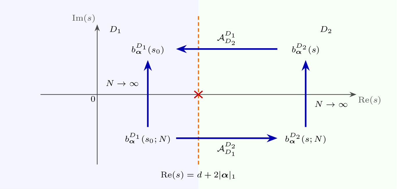
To compute the limit of \(b^h_{\boldsymbol{\alpha}}\) as \(h\rightarrow 0^+\) for a given \(\boldsymbol{\alpha}\in \mathbb{N}^d\), we introduce two sets in the complex plane \(\mathbb{C}\). For brevity, set \[s_{\boldsymbol{\alpha}}:=d+2| \boldsymbol{\alpha} |_1.\] We define \[\begin{align} D_1 &= \left\{ s \in \mathbb{C}\, : \, 0 < \mathrm{Re}(s) < s_{\boldsymbol{\alpha}} \right\}, \\ D_2 &= \left\{ s \in \mathbb{C}\, : \, s_{\boldsymbol{\alpha}} \leq \mathrm{Re}(s) < s_{\boldsymbol{\alpha}} + 1 \right\} \setminus \{s_{\boldsymbol{\alpha}}\}. \end{align}\] Their union \[D_1\cup D_2 = \left\{s\in\mathbb{C}:0<\mathrm{Re}(s)<s_{\boldsymbol{\alpha}}+1\right\} \setminus \{s_{\boldsymbol{\alpha}}\}\] is the connected open set through which the analytic continuation is performed.
By 2, the limit of \(b^h_{\boldsymbol{\alpha}}\) as \(h\to0^+\) exists. Since this limit is unique, it can be identified along any sequence \(h\to0^+\). We choose the admissible mesh sizes \(h=a/N\) and let \(N\to\infty\), which gives \[\label{eq:def95b95alpha} b_{\boldsymbol{\alpha}}^{D_1}(s) = \lim_{N\rightarrow \infty} \left( \int_{\mathbb{R}^d} g(\boldsymbol{x}\frac{a}{N}) \frac{\boldsymbol{x}^{2\boldsymbol{\alpha}}}{|\boldsymbol{x}|^s} \mathrm{d}\boldsymbol{x} - \sum_{| \boldsymbol{i} |_\infty=1}^{\infty} g(\boldsymbol{i}\frac{a}{N}) \frac{\boldsymbol{i}^{2\boldsymbol{\alpha}}}{|\boldsymbol{i}|^s} \right), \quad s \in D_1.\tag{8}\] To examine this limit, since \(\operatorname{supp}(g)\subset[-a,a]^d\), we introduce the partial expressions \[u_N^{D_1}(s) := \int_{\mathbb{R}^d} g(\boldsymbol{x}\frac{a}{N}) \frac{\boldsymbol{x}^{2\boldsymbol{\alpha}}}{|\boldsymbol{x}|^s} \mathrm{d}\boldsymbol{x}, \quad v_N^{D_1}(s) := \sum_{| \boldsymbol{i} |_\infty=1}^{N} g(\boldsymbol{i}\frac{a}{N}) \frac{\boldsymbol{i}^{2\boldsymbol{\alpha}}}{|\boldsymbol{i}|^s}.\] A key observation is that, for any fixed \(N\), the integral \(u_N^{D_1}(s)\) converges only for \(\mathrm{Re}(s) < d + 2| \boldsymbol{\alpha} |_1\), whereas the summation \(v_N^{D_1}(s)\) is well-defined for all \(s\in D_1 \cup D_2\).
Lemma 4. The function \[b_{\boldsymbol{\alpha}}^{D_1}(s) = \lim_{N\rightarrow \infty} \left( \left[u_N^{D_1} - v_N^{D_1}\right](s) \right)\] is analytic on \(D_1\).
Lemma 5. The function \(b_{\boldsymbol{\alpha}}^{D_1}(s)\) possesses an analytic continuation over \(D_1 \cup D_2\) and we have \[b_{\boldsymbol{\alpha}}^{D_2}(s) := \mathcal{A}_{D_1}^{D_2}\left[b_{\boldsymbol{\alpha}}^{D_1}\right](s) = \mathcal{A}_{D_1}^{D_2} \left[ \lim_{N\rightarrow \infty} \left( u_N^{D_1} - v_N^{D_1} \right) \right] (s) = \lim_{N\rightarrow \infty} \left( \mathcal{A}_{D_1}^{D_2} \left[u_N^{D_1} - v_N^{D_1}\right](s) \right).\]
Moreover, we introduce another domain \(D_3 \subseteq D_2\) that removes the line \(\{s \in \mathbb{C}: \mathrm{Re}(s) = s_{\boldsymbol{\alpha}}\}\), defined as \[D_3 = \left\{ s \in \mathbb{C}\, : \, s_{\boldsymbol{\alpha}} < \mathrm{Re}(s) < s_{\boldsymbol{\alpha}} + 1 \right\}.\] The purpose of introducing \(D_3\) is to avoid the line containing the pole, so that we have a simple expression of \(b^{D_3}_{\boldsymbol{\alpha}}(s)\) over \(D_3\) (such an expression is only well-defined on \(D_3\)).
Lemma 6. For \(s \in D_3\), there is \[b_{\boldsymbol{\alpha}}^{D_3}(s) = \lim_{N\rightarrow\infty} \left( \mathcal{A}_{D_1}^{D_3}[u_N^{D_1}](s) - \mathcal{A}_{D_1}^{D_3}[v_N^{D_1}](s) \right) = - \lim_{N\rightarrow\infty} \mathcal{A}_{D_1}^{D_3}[v_N^{D_1}](s) = - \sum_{| \boldsymbol{i} |_\infty=1}^{\infty} \frac{\boldsymbol{i}^{2\boldsymbol{\alpha}}}{|\boldsymbol{i}|^s}.\]
Corollary 1. For \(s \in D_1\), there is \[b_{\boldsymbol{\alpha}}^{D_1}(s) = \mathcal{A}_{D_3}^{D_1}[b_{\boldsymbol{\alpha}}^{D_3}](s) = \mathcal{A}_{D_3}^{D_1} \left[ -\sum_{| \boldsymbol{i} |_\infty=1}^{\infty} \frac{\boldsymbol{i}^{2\boldsymbol{\alpha}}}{|\boldsymbol{i}|^s} \right](s).\]
For ease of understanding, we illustrate the above analytic-continuation procedure at a point \(s_0\in D_1\cap\mathbb{R}\) in 2.
In order to compute the corrected weights, we will derive an explicit expression of \(b_{\boldsymbol{\alpha}}^{D_1}(s)\), which is a generalized zeta function (up to sign). Define \[Z_{2\boldsymbol{\alpha}}(s) := \sum_{\boldsymbol{n}\in \mathbb{Z}^{d} \setminus \{\boldsymbol{0}\}} \frac{\boldsymbol{n}^{2\boldsymbol{\alpha}}}{|\boldsymbol{n}|^s}, \quad \mathrm{Re}(s) > d+2| \boldsymbol{\alpha} |_1.\] In one dimensional scenario, it happens to be \(2\zeta(s-2| \boldsymbol{\alpha} |_1)\), where \(\zeta(s)\) is the well-known Riemann zeta function. In higher dimension, the case \(\boldsymbol{\alpha}=\boldsymbol{0}\) reduces to the Epstein zeta function [20]–[22], which has a meromorphic continuation to the whole complex plane \(\mathbb{C}\) with the only simple pole \(s=d\). Following the idea of Riemann, we derive a functional equation for \(Z_{2\boldsymbol{\alpha}}(s)\) that yields its meromorphic continuation and a rapidly convergent series representation for numerical evaluation.
Theorem 1. For generalized zeta function defined as \[Z_{2\boldsymbol{\alpha}}(s) := \sum_{\boldsymbol{n}\in \mathbb{Z}^{d} \setminus \{\boldsymbol{0}\}} \frac{\boldsymbol{n}^{2\boldsymbol{\alpha}}}{|\boldsymbol{n}|^s}, \quad \mathrm{Re}(s) > d+2| \boldsymbol{\alpha} |_1,\] it has a meromorphic continuation to the whole complex plane \(\mathbb{C}\) with the only simple pole at \(s=d+2| \boldsymbol{\alpha} |_1\), and satisfies the functional equation \[\label{eq:zeta95func95equation} \begin{align} \frac{\Gamma(s/2)}{\pi^{s/2}} Z_{2\boldsymbol{\alpha}}(s) &= \left(-\frac{1}{4\pi}\right)^{| \boldsymbol{\alpha} |_1} \frac{2H_{2\boldsymbol{\alpha}}(0)}{s - d - 2| \boldsymbol{\alpha} |_1} - \frac{2\delta_{0, \boldsymbol{\alpha}}}{s} + \sum_{\boldsymbol{n}\in \mathbb{Z}^d \setminus \{\boldsymbol{0}\}} \boldsymbol{n}^{2\boldsymbol{\alpha}} \int_{1}^{\infty} \mathrm{e}^{-|\boldsymbol{n}|^2\pi t} \, t^{\frac{s}{2} -1} \mathrm{d}t \\ &\quad + \left(-\frac{1}{4\pi}\right)^{| \boldsymbol{\alpha} |_1} \sum_{\boldsymbol{k}\in \mathbb{Z}^d \setminus \{\boldsymbol{0}\}} \int_{1}^{\infty} \mathrm{e}^{-|\boldsymbol{k}|^2 \pi t} H_{2\boldsymbol{\alpha}}(\sqrt{\pi t} \, \boldsymbol{k}) \, t^{\frac{d + 2 | \boldsymbol{\alpha} |_1 - s}{2} - 1} \mathrm{d}t, \end{align}\qquad{(2)}\] where \(H_{2\boldsymbol{\alpha}}(\boldsymbol{x})\) is the multivariate Hermite polynomial in order \(2\boldsymbol{\alpha}\) defined in 2.
For numerical evaluation, it is useful to rewrite the integral terms in ?? using the upper incomplete Gamma function \[\Gamma(s, x) := \int_x^{\infty} t^{s-1} \mathrm{e}^{-t} \,\mathrm{d}t, \quad \text{for } s\in\mathbb{C}, \, x>0.\] For \(s\in\mathbb{C}\) and \(x>0\), the change of variables \(u=tx\) gives \[\int_{1}^{\infty} t^{s - 1} \mathrm{e}^{-tx} \mathrm{d}t = \frac{1}{x^s} \, \Gamma(s, x).\] Applying this identity to the first integral series in ?? yields \[\label{eq:zeta95series95n} \begin{align} \sum_{| \boldsymbol{n} |_\infty=1}^{\infty} \boldsymbol{n}^{2\boldsymbol{\alpha}} \int_{1}^{\infty} \mathrm{e}^{-|\boldsymbol{n}|^2\pi t} \, t^{\frac{s}{2} -1} \,\mathrm{d}t &= \sum_{| \boldsymbol{n} |_\infty=1}^{\infty} \boldsymbol{n}^{2\boldsymbol{\alpha}} \frac{1}{|\boldsymbol{n}|^s \pi^{s/2}} \Gamma(\frac{s}{2}, |\boldsymbol{n}|^2 \pi) \\ &= \frac{1}{\pi^{s/2}} \sum_{| \boldsymbol{n} |_\infty=1}^{\infty} \left(\frac{\boldsymbol{n}}{|\boldsymbol{n}|}\right)^{2\boldsymbol{\alpha}} \frac{1}{|\boldsymbol{n}|^{s-2| \boldsymbol{\alpha} |_1}} \Gamma(\frac{s}{2}, |\boldsymbol{n}|^2 \pi). \end{align}\tag{9}\] For the second integral series, we first expand \(H_{2\boldsymbol{\alpha}}(\boldsymbol{x}) = \sum_{0 \leq | \boldsymbol{\beta} |_1 \leq 2| \boldsymbol{\alpha} |_1} c_{\boldsymbol{\beta}} \boldsymbol{x}^{\boldsymbol{\beta}}\) and then apply the same identity of incomplete Gamma function term by term. This gives \[\begin{gather} \label{eq:zeta95series95k} \sum_{| \boldsymbol{k} |_\infty=1}^{\infty} \int_{1}^{\infty} \mathrm{e}^{-|\boldsymbol{k}|^2 \pi t} H_{2\boldsymbol{\alpha}}(\sqrt{\pi t} \, \boldsymbol{k}) \, t^{\frac{d+2| \boldsymbol{\alpha} |_1-s}{2} - 1} \,\mathrm{d}t \\ = \pi^{\frac{s-d-2| \boldsymbol{\alpha} |_1}{2}} \sum_{0 \leq | \boldsymbol{\beta} |_1 \leq 2| \boldsymbol{\alpha} |_1} c_{\boldsymbol{\beta}} \sum_{| \boldsymbol{k} |_\infty=1}^{\infty} \left( \frac{\boldsymbol{k}}{|\boldsymbol{k}|} \right)^{\boldsymbol{\beta}} \frac{1}{|\boldsymbol{k}|^{d+2| \boldsymbol{\alpha} |_1-s}} \Gamma\!\left(\frac{| \boldsymbol{\beta} |_1+d +2| \boldsymbol{\alpha} |_1 -s}{2}, |\boldsymbol{k}|^2 \pi\right). \end{gather}\tag{10}\]
The series in representations 9 and 10 are rapidly convergent because the incomplete Gamma factors decay exponentially in the lattice index. The following tail estimate quantifies this decay and can be used to choose a finite summation cutoff.
Corollary 2. Given \(a, b \in \mathbb{R}\), for \(N \in \mathbb{N}\) such that \(\pi N^2 \geq \max\left\{a, 1, \frac{2a+b+d}{2}\right\}\), we have \[\sum_{| \boldsymbol{n} |_\infty=N+1}^{\infty} |\boldsymbol{n}|^{b} \, \Gamma(a, |\boldsymbol{n}|^2 \pi) \leq 3^{d-1} \, d^{1 + \max\{0, b/2\}} \, \pi^a \cdot N^{2a+b+d} \mathrm{e}^{-\pi N^2}.\]
Proof. This is a special case of 18. ◻
In practice, this bound is used to choose the truncation range needed for a prescribed accuracy. To reduce roundoff error when summing the series, one may use Kahan summation [23]. Finally, because the linear system for the correction weights can become ill-conditioned for large \(p\), it is preferable to solve it either symbolically or using high-precision arithmetic.
2.4 The SinCoTrap quadrature rule↩︎
We now summarize the quadrature rule obtained from the preceding construction. Fix a correction order \(p\in\mathbb{N}\) and the correction stencil \[\mathcal{X}_p=\{\boldsymbol{i}\in\mathbb{Z}^d:0\leq| \boldsymbol{i} |_1\leq p\}.\] The converged correction weights \(w\) are determined by the linear system \[Aw=b,\] where for \(\boldsymbol{\alpha}, \boldsymbol{\beta}\in\mathbb{N}^d\) such that \(0\leq| \boldsymbol{\alpha} |_1, | \boldsymbol{\beta} |_1\leq p\), \[A_{\boldsymbol{\alpha},\boldsymbol{\beta}} = \sum_{\boldsymbol{i}\in\mathcal{G}_{\boldsymbol{\beta}}}\boldsymbol{i}^{2\boldsymbol{\alpha}}, \qquad b_{\boldsymbol{\alpha}}(s) = -Z_{2\boldsymbol{\alpha}}(s).\] Here \(\mathcal{G}_{\boldsymbol{\beta}} = \left\{ (\pm \beta_1, \pm \beta_2, \ldots, \pm \beta_d) \in \mathbb{Z}^d \right\}\). The weights are then extended to all \(\boldsymbol{i}\in\mathcal{X}_p\) by \(w_{\boldsymbol{i}}=w_{\boldsymbol{\beta}}\) for \(\boldsymbol{i}\in\mathcal{G}_{\boldsymbol{\beta}}\).
For \(h=a/N\), the SinCoTrap rule for \(\sigma(\boldsymbol{x})=|\boldsymbol{x}|^{-s}\) is defined as \[\label{eq:sincotrap95compact} Q^p_h[\phi \cdot \sigma] := T^0_h[\phi \cdot \sigma] + \mathcal{C}_{h}^p[\phi], \qquad \mathcal{C}_{h}^p[\phi] := h^{d-s} \sum_{\boldsymbol{i}\in \mathcal{X}_p} w_{\boldsymbol{i}}\,\phi(\boldsymbol{i}h),\tag{11}\] where \(\mathcal{C}_{h}^p[\cdot]\) is the correction operator for the singularity.
3 Convergence order analysis↩︎
This section establishes the convergence rate of the singularity corrected trapezoidal rule for singular kernel \(\sigma(\boldsymbol{x})=|\boldsymbol{x}|^{-s}\) with \(0<s<d\).
Lemma 7 (Odd-moment cancellation). Let \(g(\boldsymbol{x})=g(|\boldsymbol{x}|)\) be smooth and compactly supported in \(V=[-a,a]^d\), and let \(\sigma(\boldsymbol{x})=|\boldsymbol{x}|^{-s}\) with \(0<s<d\). If a multi-index \(\boldsymbol{\alpha}\) has at least one odd component, then, for any correction order \(p\in\mathbb{N}\), the exact integral and the numerical quadrature vanish, \[I[g\cdot\sigma\cdot\boldsymbol{x}^{\boldsymbol{\alpha}}]=0, \qquad \text{and} \qquad Q_h^p[g\cdot\sigma\cdot\boldsymbol{x}^{\boldsymbol{\alpha}}]=0.\]
Proof. Without loss of generality, suppose that \(\alpha_1\) is odd. Since \(g\) and \(\sigma\) are radial, then we have \[\begin{align} I[g\cdot\sigma\cdot\boldsymbol{x}^{\boldsymbol{\alpha}}] &=\int_{[-a,a]^{d-1}}\int_0^a g(|\boldsymbol{x}|)\sigma(|\boldsymbol{x}|) \left[x_1^{\alpha_1}+(-x_1)^{\alpha_1}\right] \prod_{j=2}^d x_j^{\alpha_j}\,\mathrm{d}x_1\cdots\mathrm{d}x_d =0. \end{align}\] Similarly, using \(c_{(i_1,i_2,\ldots,i_d)}=c_{(-i_1,i_2,\ldots,i_d)}\), we obtain \[\begin{align} T_h^0[g\cdot\sigma\cdot\boldsymbol{x}^{\boldsymbol{\alpha}}] &=h^d\sum_{i_2=-N}^N\cdots\sum_{i_d=-N}^N \sum_{i_1=1}^N c_{\boldsymbol{i}}\,g(|\boldsymbol{i}h|)\sigma(|\boldsymbol{i}h|) \left[(i_1h)^{\alpha_1}+(-i_1h)^{\alpha_1}\right] \prod_{j=2}^d(i_jh)^{\alpha_j} =0. \end{align}\] For every sign-orbit \(\mathcal{G}_{\boldsymbol{\beta}}\), the symmetry condition 4 gives \[\sum_{\boldsymbol{i}\in\mathcal{G}_{\boldsymbol{\beta}}}(\boldsymbol{i}h)^{\boldsymbol{\alpha}} =\frac{1}{2}\sum_{\boldsymbol{i}\in\mathcal{G}_{\boldsymbol{\beta}}} \left[(\boldsymbol{i}h)^{\boldsymbol{\alpha}} +((-i_1,i_2,\ldots,i_d)h)^{\boldsymbol{\alpha}}\right]=0.\] Consequently, the correction \(\mathcal{C}_h^p[g\cdot\boldsymbol{x}^{\boldsymbol{\alpha}}]\) is zero and we conclude that \(Q_h^p[g\cdot\sigma\cdot\boldsymbol{x}^{\boldsymbol{\alpha}}]=0\). ◻
Now we state the main theorem regarding the convergence order of SinCoTrap for compactly supported singular integrals.
Theorem 2. Let \(V=[-a,a]^d\subseteq\mathbb{R}^d\) and consider \[I[\phi \cdot \sigma] = \int_{V} \phi(\boldsymbol{x})\sigma(\boldsymbol{x})\,\mathrm{d}\boldsymbol{x}, \qquad \sigma(\boldsymbol{x})=\frac{1}{|\boldsymbol{x}|^s}, \qquad 0<s<d,\] where \(\phi\) is smooth and compactly supported in \(V\). For a correction order \(p\in\mathbb{N}\), let \(Q_h^p[\cdot]\) be the SinCoTrap rule defined in 11 . Then, as \(h\to0^+\), \[I[\phi \cdot \sigma] = Q^p_h[\phi \cdot \sigma] + O(h^{2p+2+d-s}).\]
Proof. Let \(P_{\phi}(\boldsymbol{x})\) be the Taylor polynomial of \(\phi(\boldsymbol{x})\) at \(\boldsymbol{x}=0\) of degree \(2p+1\) and define the localized surrogate as \[\tilde{\phi}(\boldsymbol{x}) := P_{\phi}(\boldsymbol{x}) g(\boldsymbol{x}), \quad P_{\phi}(\boldsymbol{x}) := \sum_{| \boldsymbol{\alpha} |_1 = 0}^{2p+1} \frac{\partial^{\boldsymbol{\alpha}} \phi(0)}{\boldsymbol{\alpha}!} \boldsymbol{x}^{\boldsymbol{\alpha}},\] where \(g(\boldsymbol{x}) \in C_c^{\infty}(\mathbb{R}^d)\) is compactly supported in domain \(V\) such that \[g(\boldsymbol{x})=g(|\boldsymbol{x}|),\qquad g(0)=1,\qquad \partial^{\boldsymbol{\alpha}}g(0)=0, \quad 1\leq | \boldsymbol{\alpha} |_1\leq 2p+1.\] Decompose the quadrature error of the singular integral as: \[\begin{align} I[\phi \cdot \sigma] - Q_h^p[\phi \cdot \sigma] &= (I - T^0_h) [(\phi - \tilde{\phi}) \cdot \sigma] + \mathcal{C}_{h}^p[\tilde{\phi}- \phi] + (I - Q_h^p)[\tilde{\phi}\cdot \sigma] \\ &:= E_1 + E_2 + E_3. \end{align}\]
For \(E_1\), denote \(f:= \phi - \tilde{\phi}\), then by direct calculation we have \[\label{eq:diff95phi95tphi} f(0) = 0, \quad \partial^{\boldsymbol{\alpha}} f(0) = 0, \quad \text{for } 1 \leq | \boldsymbol{\alpha} |_1 \leq 2p+1.\tag{12}\] Thus, using the fact that \(f \in C^{\infty}_{\text{c}}(V)\), we can write \[\begin{align} E_1 = I[f\cdot \sigma] - T^0_h[f \cdot \sigma] &= \int_{[-a, a]^d} f(\boldsymbol{x}) \frac{1}{|\boldsymbol{x}|^s} \mathrm{d}\boldsymbol{x} - \sum_{| \boldsymbol{i} |_\infty=1}^N h^d f(\boldsymbol{i}h) \frac{1}{|\boldsymbol{i}h|^s} \\ &= h^{d-s} \Big( \int_{\mathbb{R}^d} f(\boldsymbol{x}h) \frac{1}{|\boldsymbol{x}|^s} \mathrm{d}\boldsymbol{x} - \sum_{| \boldsymbol{i} |_\infty=1}^{\infty} f(\boldsymbol{i}h) \frac{1}{|\boldsymbol{i}|^s} \Big) = O(h^{2p+2+d-s}), \end{align}\] where we used 2 with \(\boldsymbol{\alpha}=\boldsymbol{0}\) and \(f(0)=0\) in the last step.
For \(E_2\), note that Taylor’s theorem with 12 gives \(|\tilde{\phi}(\boldsymbol{x})-\phi(\boldsymbol{x})|\leq C|\boldsymbol{x}|^{2p+2}\) on \(V\), hence on the fixed stencil \(\mathcal{X}_p\) with bounded weights, we have \[|E_2| \leq h^{d-s}\sum_{\boldsymbol{i}\in\mathcal{X}_p} |w_{\boldsymbol{i}}|\,|\tilde{\phi}(\boldsymbol{i}h)-\phi(\boldsymbol{i}h)| \leq C h^{2p+2+d-s}.\]
For \(E_3\), expand \(\tilde{\phi}=P_\phi g\) and use 7 to drop the odd monomials we obtain \[(I-Q_h^p)[\tilde{\phi}\cdot\sigma] = \sum_{| \boldsymbol{\alpha} |_1=0}^{p}\frac{\partial^{2\boldsymbol{\alpha}}\phi(0)}{(2\boldsymbol{\alpha})!}\, (I-Q_h^p)[\boldsymbol{x}^{2\boldsymbol{\alpha}}g\cdot\sigma].\] For each even monomial above, according to the moment conditions 3 we have \[I[\boldsymbol{x}^{2\boldsymbol{\alpha}}g\cdot\sigma] - T_h^0[\boldsymbol{x}^{2\boldsymbol{\alpha}}g\cdot\sigma] = h^{d-s}\sum_{\boldsymbol{i}\in\mathcal{X}_p} w_{\boldsymbol{i}}^h\,(\boldsymbol{i}h)^{2\boldsymbol{\alpha}}g(\boldsymbol{i}h).\] On the other hand, the SinCoTrap rule \(Q_h^p\) uses the converged weights \(w_{\boldsymbol{i}}\), so \[(I-Q_h^p)[\boldsymbol{x}^{2\boldsymbol{\alpha}}g\cdot\sigma] = \left(I-T_h^0\right)[\boldsymbol{x}^{2\boldsymbol{\alpha}}g\cdot\sigma] - h^{d-s}\sum_{\boldsymbol{i}\in\mathcal{X}_p} w_{\boldsymbol{i}}\,(\boldsymbol{i}h)^{2\boldsymbol{\alpha}}g(\boldsymbol{i}h).\] Substituting the moment identity gives \[(I-Q_h^p)[\boldsymbol{x}^{2\boldsymbol{\alpha}}g\cdot\sigma] = h^{d-s}\sum_{\boldsymbol{i}\in\mathcal{X}_p} (w_{\boldsymbol{i}}^h-w_{\boldsymbol{i}})\,(\boldsymbol{i}h)^{2\boldsymbol{\alpha}}g(\boldsymbol{i}h).\] Thus, by 3 we have \[\begin{align} |E_3| \leq C h^{d-s} \sum_{| \boldsymbol{\alpha} |_1 = 0}^{p} \sum_{\boldsymbol{i}\in \mathcal{X}_p} \left|(\boldsymbol{i}h)^{2\boldsymbol{\alpha}} g(\boldsymbol{i}h)\right| \left| w_{\boldsymbol{i}}^h - w_{\boldsymbol{i}} \right| \leq C h^{2p+2+d-s}. \end{align}\]
Combining the three bounds yields the claim. ◻
Remark 3. The assumption that \(\phi\) is smooth is imposed only for convenience; the argument requires only finitely many derivatives. In particular, it suffices to assume that \(\phi\in C_c^{d+2p+3}(V)\) and to use the corresponding finite-regularity version of 2, obtained by applying Poisson summation to finitely differentiable, compactly supported functions. This regularity threshold is sufficient and may not be optimal.
Remark 4. Replacing \(w_{\boldsymbol{i}}\) by the non-converged weights \(w_{\boldsymbol{i}}^h\) removes the term \(E_3\) above, but \(E_1\) and \(E_2\) still scale like \(h^{2p+2+d-s}\), so the overall order remains unchanged.
Next we give the convergence rate for singular integrals satisfying the smooth periodic boundary conditions.
Corollary 3. Let \(V=[-a,a]^d\subseteq\mathbb{R}^d\) and consider \[I[\varphi\cdot \sigma] = \int_V \varphi(\boldsymbol{x})\sigma(\boldsymbol{x})\,\mathrm{d}\boldsymbol{x}, \qquad \sigma(\boldsymbol{x})=\frac{1}{|\boldsymbol{x}|^s}, \qquad 0<s<d,\] where \(\varphi(\boldsymbol{x})\) is smooth, \(\varphi(\boldsymbol{x})\sigma(\boldsymbol{x})\) is periodic on \(V\) and is smooth except at the singular points. For a correction order \(p\in\mathbb{N}\), let \(Q_h^p[\cdot]\) be the SinCoTrap rule defined in 11 . Then, as \(h\to0^+\), \[I[\varphi\cdot \sigma] = Q^p_h[\varphi\cdot \sigma] + O(h^{2p+2+d-s}).\]
Proof. Using the smooth cutoff \(\eta\) defined in 1 , we split the integral as \[I[\varphi\cdot \sigma] = I[\varphi\cdot \sigma \cdot \eta] + I[\varphi\cdot \sigma \cdot (1 - \eta)].\] For the first term, since \(\varphi(\boldsymbol{x})\eta(\boldsymbol{x})\) is smooth and compactly supported in \(V\), 2 implies \[I[\varphi\cdot \sigma \cdot \eta] = T^0_h[\varphi\cdot \sigma \cdot \eta] + \mathcal{C}_{h}^p[\varphi\cdot \eta] + O(h^{2p+2+d-s}).\] For the second term, since \(\varphi(\boldsymbol{x}) \sigma(\boldsymbol{x}) (1 - \eta(\boldsymbol{x}))\) is \(0\) at \(x=0\), the punctured trapezoidal rule is equivalent to the standard trapezoidal rule. Moreover, since \(\varphi(\boldsymbol{x}) \sigma(\boldsymbol{x}) (1 - \eta(\boldsymbol{x}))\) is smooth and periodic with respect to the domain \(V\), the Euler-Maclaurin formula yields \[I[\varphi\cdot \sigma \cdot (1 - \eta)] = T^0_h[\varphi\cdot \sigma \cdot (1 - \eta)] + O(h^{q}),\] for any \(q>0\). Finally, note that \(\mathcal{C}_{h}^p[\varphi\cdot \eta] = \mathcal{C}_{h}^p[\varphi]\) for \(h>0\) sufficient small, we have \[\begin{align} I[\varphi\cdot \sigma] &= T^0_h[\varphi\cdot \sigma \cdot \eta] + \mathcal{C}_{h}^p[\varphi\cdot \eta] + O(h^{2p+2+d-s}) + T^0_h[\varphi\cdot \sigma \cdot (1 - \eta)] + O(h^{q}) \\ &= T^0_h[\varphi\cdot \sigma] + \mathcal{C}_{h}^p[\varphi] + O(h^{2p+2+d-s}), \end{align}\] which completes the proof. ◻
4 Extensions↩︎
In this section, we present two extensions of the SinCoTrap. First, we extend the method to integrals with singular kernel \(1/|\boldsymbol{x}^\top B \boldsymbol{x}|^{s/2}\), where \(B\) is a symmetric positive definite matrix. Second, we extend the method to integrals over general bounded domains, specifically parallelotopes. We note that these two extensions are equivalent under a linear transformation and they find applications in electronic structure calculations for solids with parallelepiped-shaped unit cells.
4.1 Extension to anisotropic singular kernel↩︎
We begin with an anisotropic singular kernel induced by a symmetric positive definite matrix \(B \in \mathbb{R}^{d\times d}\). Consider \[I[\phi \cdot \sigma_B] = \int_{V} \phi(\boldsymbol{x}) \sigma_B(\boldsymbol{x}) \mathrm{d}\boldsymbol{x}, \quad \sigma_B(\boldsymbol{x}) = \frac{1}{|\boldsymbol{x}^\top B \boldsymbol{x}|^{s/2}} \quad 0 < s < d,\] where \(V=[-a, a]^d\), \(\phi(\boldsymbol{x})\) is smooth and compactly supported in \(V\). Since \(B\) is invertible, the only singular point of \(I[\phi \cdot \sigma_B]\) remains at \(\boldsymbol{x}=0\). For discretization, we employ the same uniform grid used for the isotropic kernel \(\sigma(\boldsymbol{x})=1/|\boldsymbol{x}|^s\).
4.1.0.1 Central symmetry and moment constraints.
Since the singular kernel is changed, the local correction weights must be recomputed accordingly. In contrast to the isotropic kernel \(|\boldsymbol{x}|^{-s}\), the anisotropic kernel \(\sigma_B(\boldsymbol{x})\) is generally not radially symmetric (unless \(B\) is a scalar multiple of the identity). It retains only central symmetry \[\sigma_B(-\boldsymbol{x})=\sigma_B(\boldsymbol{x}),\] since \(\boldsymbol{x}^\top B \boldsymbol{x}= (-\boldsymbol{x})^\top B (-\boldsymbol{x})\). This reduced symmetry affects both the design of the correction stencil \(\mathcal{X}_p\) and which moment constraints are automatically satisfied.
Following the moment-matching construction in 2, we again determine the correction weights by requiring exactness on localized monomials \(g(\boldsymbol{x})\sigma_B(\boldsymbol{x})\boldsymbol{x}^{\boldsymbol{\alpha}}\). Accordingly, we assume the correction stencil \(\mathcal{X}_p\subset\mathbb{Z}^d\) is centrally symmetric and contains the origin, i.e., \(\boldsymbol{i}\in\mathcal{X}_p\) implies \(-\boldsymbol{i}\in\mathcal{X}_p\) and \(0\in\mathcal{X}_p\), and we impose the same symmetry on the weights: \[w_{-\boldsymbol{i}}^h = w_{\boldsymbol{i}}^h.\] These weights are determined by enforcing, for \(0\le | \boldsymbol{\alpha} |_1\le 2p+1\), \[\int_V g(\boldsymbol{x})\sigma_B(\boldsymbol{x})\boldsymbol{x}^{\boldsymbol{\alpha}}\,\mathrm{d}\boldsymbol{x} = T^0_h[g \cdot \sigma_B \cdot \boldsymbol{x}^{\boldsymbol{\alpha}}] + a(h) \sum_{\boldsymbol{i}\in \mathcal{X}_p} w_{\boldsymbol{i}}^h \, (\boldsymbol{i}h)^{\boldsymbol{\alpha}} \, g(\boldsymbol{i}h).\] As in the isotropic case, we choose a radial localized function \(g\in C_c^{\infty}(V)\) such that \(g(0)=1\) and \(\partial^{\boldsymbol{\beta}}g(0)=0\) for \(1\leq | \boldsymbol{\beta} |_1\leq 2p+1\).
With only central symmetry, the automatic cancellation applies to monomials of odd total degree: if \(| \boldsymbol{\alpha} |_1\) is odd, then both the integral and the corrected rule vanish (see 8). In contrast, monomials with \(| \boldsymbol{\alpha} |_1\) even but with at least one odd component are not forced to vanish in general. Therefore, the moment-matching system must include all multi-indices with even total degree, \[| \boldsymbol{\alpha} |_1=2q,\quad \text{for } q=0,1,\ldots,p,\] which determines the number of independent constraints (and hence the number of independent weights).
4.1.0.2 Stencil choice and linear system.
As discussed above, in the anisotropic case the symmetry only forces cancellation of moments with odd total degree. Hence, to obtain a square moment-matching system we choose the stencil so that the number of independent weights matches the number of even-total-degree moment conditions, i.e., \(N_w\).
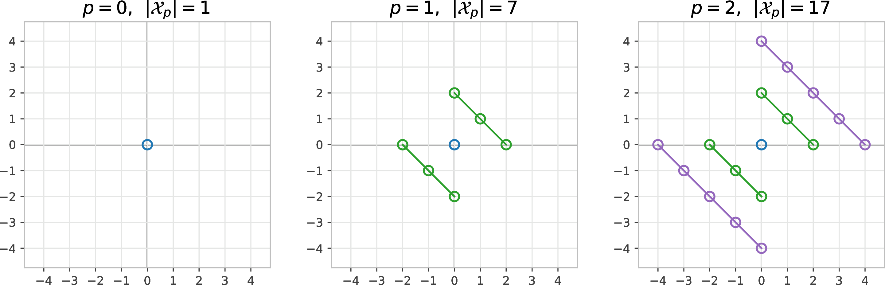
A convenient way is to take one representative in the nonnegative orthant for each multi-index of even total degree up to \(2p\) and then include its negative. Specifically, define \[\mathcal{X}_p := \mathcal{X}_p^{+} \cup \mathcal{X}_p^{-}, \qquad \mathcal{X}_p^+ := \left\{ \boldsymbol{\beta}\in \mathbb{N}^d : | \boldsymbol{\beta} |_1 \leq 2p,\;| \boldsymbol{\beta} |_1\;\text{even} \right\}, \qquad \mathcal{X}_p^- := -\mathcal{X}_p^+.\] Since every nonzero point in \(\mathcal{X}_p^+\) is paired with its negative in \(\mathcal{X}_p^-\), and conversely, thus the full stencil \(\mathcal{X}_p\) is centrally symmetric. We impose the central symmetry \(w_{-\boldsymbol{\beta}}^h=w_{\boldsymbol{\beta}}^h\), so the independent unknowns can be taken as \(\{w_{\boldsymbol{\beta}}^h\}_{\boldsymbol{\beta}\in\mathcal{X}_p^+}\). (Here the origin is included in \(\mathcal{X}_p^+\) and is not duplicated by the sign pairing.) For illustration, we plot the correction stencils \(\mathcal{X}_p\) for \(p=0,1,2\) in two dimensions in 3.
Remark 5. The stencil above is a simple and convenient choice but not unique. Any alternative stencil can be used provided that:
it is centrally symmetric and contains the origin;
the number of independent weights (after enforcing \(w_{-\boldsymbol{i}}^h=w_{\boldsymbol{i}}^h\)) matches the number of even-total-degree moment constraints, i.e., \(\#\mathcal{X}_p^+ = N_w\);
the resulting matrix for moment matching is nonsingular.
Now we derive the matrix form of the moment-matching system. The scaling factor remains \(a(h)=h^{d-s}\) by the same homogeneity argument as in 2. Order the even-total-degree moment indices as \(\boldsymbol{\alpha}_1,\ldots,\boldsymbol{\alpha}_{N_w}\) and the independent stencil nodes in \(\mathcal{X}_p^+\) as \(\boldsymbol{\beta}_1,\ldots,\boldsymbol{\beta}_{N_w}\) with the same ordering. Then the moment conditions become \[\sum_{k=1}^{N_w} w_{\boldsymbol{\beta}_k}^h \sum_{\boldsymbol{i}\in \{\boldsymbol{\beta}_k, -\boldsymbol{\beta}_k\}} \boldsymbol{i}^{\boldsymbol{\alpha}_j}\, g(\boldsymbol{i}h) = \int_{\mathbb{R}^d} g(\boldsymbol{x}h)\sigma_B(\boldsymbol{x})\boldsymbol{x}^{\boldsymbol{\alpha}_j}\,\mathrm{d}\boldsymbol{x} - \sum_{| \boldsymbol{i} |_\infty=1}^{\infty} g(\boldsymbol{i}h)\sigma_B(\boldsymbol{i})\boldsymbol{i}^{\boldsymbol{\alpha}_j} := b_j^h,\] for \(j=1,2,\ldots,N_w\). As in 2, it is convenient to introduce \[\label{eq:matrix95of95scaled95zeta} A_{jk} := \sum_{\boldsymbol{i}\in \{\boldsymbol{\beta}_k, -\boldsymbol{\beta}_k\}} \boldsymbol{i}^{\boldsymbol{\alpha}_j}, \qquad (G^h)_{jk} := g(\boldsymbol{\beta}_k h)\delta_{jk},\tag{13}\] Then the system becomes \[A G^h w^h = b^h.\]
Remark 6. It is tempting to reuse the sign-orbit (radial-symmetry) grouping from the isotropic case. However, once the constraint set includes a multi-index \(\boldsymbol{\alpha}\) with \(| \boldsymbol{\alpha} |_1\) even but with at least one odd component, the corresponding row in the coefficient matrix defined as \(A_{jk} := \sum_{\boldsymbol{i}\in \mathcal{G}_{\boldsymbol{\beta}_k}} \boldsymbol{i}^{\boldsymbol{\alpha}_j}\) becomes zero under sign-orbit summation, making the system singular and thus the right-hand side vector no longer lies in the spanned space of \(A\). This is precisely why we switch to a merely centrally symmetric stencil in the anisotropic setting.
In practice, for a given choice of stencil \(\mathcal{X}_p\), the nonsingularity of the resulting moment matrix \(A\) can be checked directly. Since every entry of \(A\) is an integer, \(\det(A)\in\mathbb{Z}\) as well, and it can therefore be computed exactly using integer arithmetic (thus avoiding roundoff issues). Although exact determinant computation has cost that grows rapidly with the matrix size, this check remains very fast for the moderate values of \(p\) used in practice.
4.1.0.3 Weight computation.
The limiting weights \(w_{\boldsymbol{i}}=\lim_{h\to 0^+} w_{\boldsymbol{i}}^h\) can be defined by passing to the limit \(h\to 0^+\), and the convergence analysis follows similarly to 2. Furthermore, the right-hand side can be evaluated using analytic continuation through a generalized zeta function associated with matrix \(B\).
Theorem 3. For any symmetric positive definite matrix \(B \in \mathbb{R}^{d\times d}\), define \[Z_{\boldsymbol{\alpha}}^B(s) := \sum_{\boldsymbol{n}\in \mathbb{Z}^{d} \setminus \{\boldsymbol{0}\}} \frac{\boldsymbol{n}^{\boldsymbol{\alpha}}}{(\boldsymbol{n}^\top B \boldsymbol{n})^{s/2}}, \quad \mathrm{Re}(s) > d + | \boldsymbol{\alpha} |_1,\] where \(| \boldsymbol{\alpha} |_1\) is an even number. Then \(Z_{\boldsymbol{\alpha}}^B(s)\) admits a meromorphic extension to the whole complex plane with at most a simple pole at \(s = d + | \boldsymbol{\alpha} |_1\). Further, it satisfies the functional equation as \[\begin{align} \frac{\Gamma(s/2)}{\pi^{s/2}} Z_{\boldsymbol{\alpha}}^B(s) &= |B|^{-\frac{1}{2}} \left(-\frac{1}{4\pi}\right)^{\frac{| \boldsymbol{\alpha} |_1}{2}} \frac{2H_{\boldsymbol{\alpha}}(0; B^{-1})}{s - d - | \boldsymbol{\alpha} |_1} - \frac{2\delta_{0, \boldsymbol{\alpha}}}{s} + \sum_{\boldsymbol{n}\in\mathbb{Z}^d \setminus \{\boldsymbol{0}\}} \boldsymbol{n}^{\boldsymbol{\alpha}} \int_{1}^{\infty} \mathrm{e}^{-\pi t \, \boldsymbol{n}^\top B \boldsymbol{n}} \, t^{\frac{s}{2} -1} \mathrm{d}t \\ &\quad + |B|^{-\frac{1}{2}} \left(-\frac{1}{4\pi}\right)^{\frac{| \boldsymbol{\alpha} |_1}{2}} \sum_{\boldsymbol{k}\in \mathbb{Z}^d \setminus \{\boldsymbol{0}\}} \int_{1}^{\infty} \mathrm{e}^{-\pi t \, \boldsymbol{k}^\top B^{-1} \boldsymbol{k}} H_{\boldsymbol{\alpha}}(\sqrt{\pi t} \, \boldsymbol{k}; B^{-1}) \, t^{\frac{d+| \boldsymbol{\alpha} |_1-s}{2} - 1} \mathrm{d}t, \end{align}\] where \(|B|\) is the determinant of \(B\) and \(H_{\boldsymbol{\alpha}}(x; B^{-1})\) is the multivariate Hermite polynomial with covariance matrix \(B^{-1}\) defined in 2.
For numerical evaluation, the two lattice series in the functional equation are evaluated by finite summation. As in the isotropic case, rewriting the integral terms with upper incomplete Gamma functions reveals exponential decay in the lattice index, and the corresponding tail bound determines a summation cutoff for a prescribed accuracy. The anisotropic estimate follows the same argument, and the detailed derivation is given in 11.
4.2 Extension to parallelotope domain↩︎
We now extend the SinCoTrap method to singular integrals over a general parallelotope with the isotropic kernel \(\sigma(\boldsymbol{x})=1/|\boldsymbol{x}|^s\). Let \(V_{\text{para}}\) be a parallelotope defined as \[\label{eq:def95parallelotope} V_{\text{para}}= \Big\{ \sum_{j=1}^d c_j \boldsymbol{v}_j \mid -1 \leq c_j \leq 1, j=1, \ldots, d \Big\},\tag{14}\] where \(\{\boldsymbol{v}_1, \ldots, \boldsymbol{v}_d\}\) are linearly independent vectors in \(\mathbb{R}^d\). Introduce a linear transformation \(\boldsymbol{x}= T \boldsymbol{y}\) such that \[[\boldsymbol{v}_1, \ldots, \boldsymbol{v}_d] = T \cdot a [\boldsymbol{e}_1, \ldots, \boldsymbol{e}_d] = T \cdot a I_d,\] where \(a>0\) and \(I_d\) is the \(d\)-by-\(d\) identity matrix, such a transformation maps the hypercube \([-a, a]^d\) to the parallelotope \(V_{\text{para}}\). Then we have \[\int_{V_{\text{para}}} \phi(\boldsymbol{x}) \frac{1}{|\boldsymbol{x}|^{s}} \mathrm{d}\boldsymbol{x} = |\det(T)| \int_{[-a, a]^d} \phi(T \boldsymbol{y}) \frac{1}{|\boldsymbol{y}^\top T^\top T \boldsymbol{y}|^{s/2}} \mathrm{d}\boldsymbol{y}.\] Thus, integration over a parallelotope with an isotropic kernel reduces to the cube integral with anisotropic kernel \(1/|\boldsymbol{y}^\top B\boldsymbol{y}|^{s/2}\) where \(B := T^\top T\). Conversely, given any symmetric positive definite matrix \(B\), one may choose \(T\) such that \(B=T^\top T\) (e.g., Cholesky factorization), to convert the cube integral with anisotropic kernel to an integral over parallelotope with isotropic kernel. Therefore, the two extensions are equivalent up to a linear change of variables.
For numerical computation, assume that each coordinate direction of the parallelotope is discretized with the same number of points \(2N+1\) with \(N \in \mathbb{N}\). We construct the grid on \(V_{\text{para}}\) by mapping the uniform grid on \([-a,a]^d\) through the linear transformation \(\boldsymbol{x}=T\boldsymbol{y}\). In particular, for \(\boldsymbol{y}_{\boldsymbol{i}}=\boldsymbol{i}h\) where \(h=a/N\), we define the corresponding points in \(V_{\text{para}}\) by \(\boldsymbol{x}_{\boldsymbol{i}}:=T\boldsymbol{y}_{\boldsymbol{i}}=T(\boldsymbol{i}h)\). The resulting quadrature rule is \[\label{eq:sincotrap95parallelotope} Q_{\text{para}}^p\!\left[\phi \cdot \frac{1}{|\boldsymbol{x}|^s}\right] = |\det(T)| \Bigl( h^d \sum_{0<| \boldsymbol{i} |_\infty\le N} c_{\boldsymbol{i}}\, \phi(\boldsymbol{x}_{\boldsymbol{i}}) \frac{1}{|\boldsymbol{x}_{\boldsymbol{i}}|^s} + h^{d-s} \sum_{\boldsymbol{i}\in\mathcal{X}_p} w_{\boldsymbol{i}}\, \phi(\boldsymbol{x}_{\boldsymbol{i}}) \Bigr),\tag{15}\] where \(c_{\boldsymbol{i}}\) are the standard coefficients of trapezoidal rule and \(\{w_{\boldsymbol{i}}\}\) are the converged SinCoTrap weights (computed once for the associated matrix \(B=T^\top T\) and parameters \(d,s,p\)).
4.3 Convergence analysis↩︎
Since the two extensions are equivalent via a linear transformation, we only present the convergence analysis for integral with singular kernel \(1/|\boldsymbol{x}^\top B \boldsymbol{x}|^{s/2}\) over the hypercube domain. The results and their proofs largely parallel to those for the isotropic case, though the anisotropy introduced by the matrix \(B\) entails more intricate notation and computations. Below, we state the main theorems, highlighting the essential modifications required to accommodate the anisotropic setting.
We begin with the basic cancellation property implied by central symmetry.
Lemma 8 (Odd total-degree cancellation). Given multi-index \(\boldsymbol{\alpha}\in \mathbb{N}^d\) with \(| \boldsymbol{\alpha} |_1\) being odd, and smooth radial function \(g(\boldsymbol{x})=g(|\boldsymbol{x}|)\) being compactly supported within \(V=[-a, a]^d\), if the correction stencil \(\mathcal{X}_p\) and weights \(\{w_{\boldsymbol{i}}\}\) satisfy central symmetry, i.e., \(\boldsymbol{i}\in\mathcal{X}_p\Rightarrow -\boldsymbol{i}\in\mathcal{X}_p\) and \(w_{-\boldsymbol{i}}=w_{\boldsymbol{i}}\), then for \(\sigma_B(\boldsymbol{x}) = |\boldsymbol{x}^\top B \boldsymbol{x}|^{-s/2}\), \[I[g \cdot \sigma_B \cdot \boldsymbol{x}^{\boldsymbol{\alpha}}] = 0, \qquad \text{and} \qquad Q_h^p[g \cdot \sigma_B \cdot \boldsymbol{x}^{\boldsymbol{\alpha}}] = 0.\]
Proof. Define \(F(\boldsymbol{x}):=g(\boldsymbol{x})\sigma_B(\boldsymbol{x})\boldsymbol{x}^{\boldsymbol{\alpha}}\). The radiality of \(g\) and the central symmetry of \(\sigma_B\) imply that \(g(-\boldsymbol{x})=g(\boldsymbol{x})\) and \(\sigma_B(-\boldsymbol{x})=\sigma_B(\boldsymbol{x})\). Moreover, since \(| \boldsymbol{\alpha} |_1\) is odd, \[(-\boldsymbol{x})^{\boldsymbol{\alpha}} =(-1)^{| \boldsymbol{\alpha} |_1}\boldsymbol{x}^{\boldsymbol{\alpha}} =-\boldsymbol{x}^{\boldsymbol{\alpha}}.\] Hence \(F(-\boldsymbol{x})=-F(\boldsymbol{x})\). Because \(V\) is centrally symmetric, \[I[g\cdot\sigma_B\cdot\boldsymbol{x}^{\boldsymbol{\alpha}}] = \int_V F(\boldsymbol{x})\,\mathrm{d}\boldsymbol{x} = \frac{1}{2}\int_V\bigl(F(\boldsymbol{x})+F(-\boldsymbol{x})\bigr)\,\mathrm{d}\boldsymbol{x} = 0.\] For the punctured trapezoidal sum, the index set \(\{\boldsymbol{i}\in\mathbb{Z}^d:0<| \boldsymbol{i} |_\infty\le N\}\) is centrally symmetric and \(c_{-\boldsymbol{i}}=c_{\boldsymbol{i}}\), hence terms cancel in pairs: \[T_h^0[g\cdot\sigma_B\cdot\boldsymbol{x}^{\boldsymbol{\alpha}}] = \frac{h^d}{2}\sum_{0<| \boldsymbol{i} |_\infty\le N} c_{\boldsymbol{i}}\Bigl(F(\boldsymbol{i}h)+F(-\boldsymbol{i}h)\Bigr)=0.\] Likewise, central symmetry of \(\mathcal{X}_p\) and \(w_{-\boldsymbol{i}}=w_{\boldsymbol{i}}\) gives \[h^{d-s}\sum_{\boldsymbol{i}\in\mathcal{X}_p} w_{\boldsymbol{i}}\,g(\boldsymbol{i}h)\,(\boldsymbol{i}h)^{\boldsymbol{\alpha}} = \frac{h^{d-s}}{2}\sum_{\boldsymbol{i}\in\mathcal{X}_p} w_{\boldsymbol{i}}\Bigl(g(\boldsymbol{i}h)(\boldsymbol{i}h)^{\boldsymbol{\alpha}}+g(-\boldsymbol{i}h)(-\boldsymbol{i}h)^{\boldsymbol{\alpha}}\Bigr)=0.\] Therefore \(Q_h^p[g\cdot\sigma_B\cdot\boldsymbol{x}^{\boldsymbol{\alpha}}]=0\). ◻
Theorem 4. Let \(V=[-a, a]^d \subseteq \mathbb{R}^d\) and consider the singular integral \[I[\phi \cdot \sigma_B] = \int_{V} \phi(\boldsymbol{x})\sigma_B(\boldsymbol{x})\,\mathrm{d}\boldsymbol{x}, \qquad \sigma_B(\boldsymbol{x}) = \frac{1}{|\boldsymbol{x}^\top B \boldsymbol{x}|^{s/2}}, \qquad 0 < s < d,\] where \(B\in\mathbb{R}^{d\times d}\) is symmetric positive definite and \(\phi\) is smooth. Assume that either \(\phi\) is compactly supported in \(V\) or \(\phi\cdot\sigma_B\) is periodic on \(V\) and is smooth expect at the singular points. Let \(Q_h^p\) be the singularity corrected trapezoidal rule constructed using the centrally symmetric stencil and the associated converged weights: \[Q^p_h[\phi \cdot \sigma_B] = T^0_h[\phi \cdot \sigma_B] + \mathcal{C}_{h}^p[\phi], \quad \mathcal{C}_{h}^p[\phi] = h^{d-s} \sum_{\boldsymbol{i}\in \mathcal{X}_p} w_{\boldsymbol{i}} \, \phi(\boldsymbol{i}h).\] Then as \(h\to0^+\) we have \[I[\phi \cdot \sigma_B] = Q^p_h[\phi \cdot \sigma_B] + O(h^{2p+2+d-s}).\]
Proof. The argument is similar to the proof of 2 after replacing \(\sigma(\boldsymbol{x})=|\boldsymbol{x}|^{-s}\) by \(\sigma_B(\boldsymbol{x})=|\boldsymbol{x}^\top B \boldsymbol{x}|^{-s/2}\). The only change is that the componentwise odd-moment cancellation (7) is replaced by the odd total-degree cancellation (8). ◻
5 Numerical results↩︎
This section validates the predicted convergence rate of SinCoTrap on a three-dimensional test from electronic structure calculations involving the singular kernel \(\sigma(\boldsymbol{x})=1/|\boldsymbol{x}|^{2}\) (\(d=3\), \(s=2\)), which arises in the computation of exchange energy. We report the relative error against a high-accuracy reference value and estimate rates from log–log slopes.
5.1 Example 1: isotropic cube↩︎
Consider the following singular integral over a cube domain \(V=[-2, 2]^3\): \[\int_{[-2, 2]^3} \phi(\boldsymbol{x}) \frac{1}{|\boldsymbol{x}|^2} \mathrm{d}\boldsymbol{x}, \quad \phi(\boldsymbol{x}) = \phi(|\boldsymbol{x}|) = \begin{cases} \exp(\frac{4}{|\boldsymbol{x}|^2 - 1}), & |\boldsymbol{x}| < 1, \\ 0, & |\boldsymbol{x}| \geq 1. \end{cases}\] \(\phi(\boldsymbol{x})\) is smooth and compactly supported in domain \(V\). Note that the singularity can be canceled by a spherical transformation, i.e., \[\label{eq:reference95value95example951} \int_{[-2, 2]^3} \phi(\boldsymbol{x}) \frac{1}{|\boldsymbol{x}|^2} \mathrm{d}\boldsymbol{x} = 4 \pi \int_{0}^1 \phi(r) \mathrm{d}r = 2 \pi \int_{-1}^1 \phi(r) \mathrm{d}r.\tag{16}\] Thus, we compute the reference value by a simple 1D trapezoidal rule with a very fine mesh.
As established in 2, SinCoTrap achieves a convergence rate of \(O(h^{2p+3})\) for \(d=3\), \(s=2\). Our numerical experiments employ correction orders \(p=0, 1, 2\) for a sequence of mesh sizes \(h\), with expected convergence rates of \(O(h^3)\), \(O(h^5)\), and \(O(h^7)\), respectively. After imposing the sign symmetry 4 , the corresponding numbers of independent correction weights are \(N_w=1,4,10\) for \(p=0,1,2\), respectively.
The left panel of 4 confirms the predicted convergence rates \(O(h^3)\), \(O(h^5)\), and \(O(h^7)\) for \(p=0,1,2\), respectively, whereas the uncorrected rule is only first-order accurate. These results demonstrate that SinCoTrap effectively compensates for the singularity and recovers the predicted high-order convergence using only a few correction weights localized near the singular point.
5.2 Example 2: parallelotope (anisotropic extension)↩︎
We consider the parallelotope \(V_{\text{para}}\) in \(\mathbb{R}^3\) defined by 14 with generating vectors \[\boldsymbol{v}_1 = \begin{pmatrix} 2 & 0 & 0 \end{pmatrix}^\top, \quad \boldsymbol{v}_2 = \begin{pmatrix} 0 & 2 & 0 \end{pmatrix}^\top, \quad \boldsymbol{v}_3 = \begin{pmatrix} 0 & 2\cos \frac{\pi}{3} & 2\sin \frac{\pi}{3} \end{pmatrix}^\top,\] and evaluate the singular integral \[\int_{V_{\text{para}}} \phi(\boldsymbol{x}) \frac{1}{|\boldsymbol{x}|^2} \mathrm{d}\boldsymbol{x}, \quad \phi(\boldsymbol{x}) = \phi(|\boldsymbol{x}|) = \begin{cases} \exp(\frac{4}{|\boldsymbol{x}|^2 - 1}), & |\boldsymbol{x}| < 1, \\ 0, & |\boldsymbol{x}| \geq 1, \end{cases}\] The support of \(\phi\) is contained in the unit ball, which lies inside \(V_{\text{para}}\). Thus, the reference value is obtained via a spherical transformation as in 16 . To discretize the integral and apply the quadrature rule 15 , we introduce the linear transformation \(\boldsymbol{x}=T\boldsymbol{y}\), where \((\boldsymbol{v}_1,\boldsymbol{v}_2,\boldsymbol{v}_3)=T(2I)\), which maps the reference cube \([-2,2]^3\) onto \(V_{\text{para}}\). We discretize each reference coordinate with \(2N+1\) points and parametric step size \(h=\frac{2}{N}\). Thus, the horizontal axis in the right panel of 4 represents the spacing \(h\) in the reference coordinates \(\boldsymbol{y}\); the corresponding physical grid increments are \(T(h\boldsymbol{e}_j)\).
For \(d=3\) and \(s=2\), 4 predicts an error of order \(O(h^{2p+3})\). We again use \(p=0,1,2\), for which the expected rates are \(O(h^3)\), \(O(h^5)\), and \(O(h^7)\), respectively. Because the transformed kernel is anisotropic, the moment system includes every multi-index of even total degree up to \(2p\). The corresponding numbers of independent correction weights are \(N_w=1,7,22\) for \(p=0,1,2\), respectively.
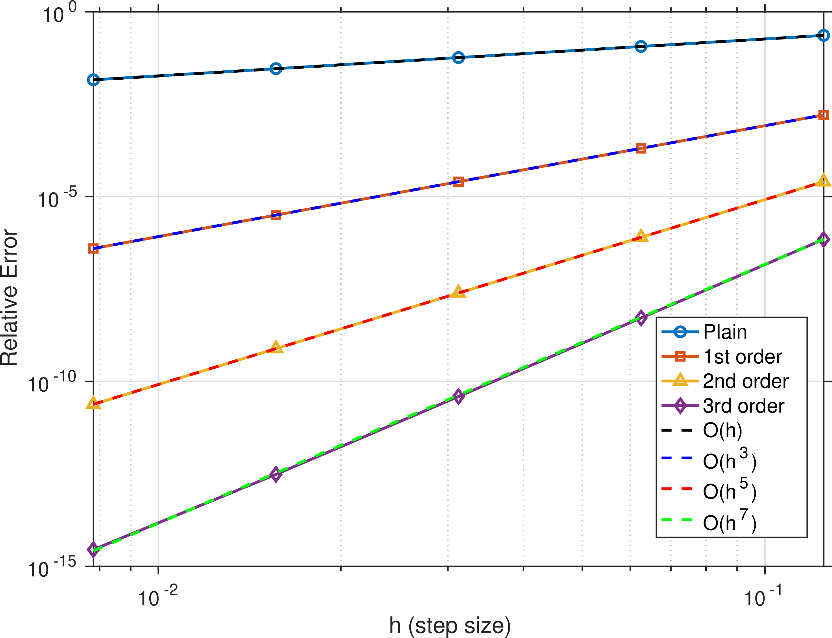
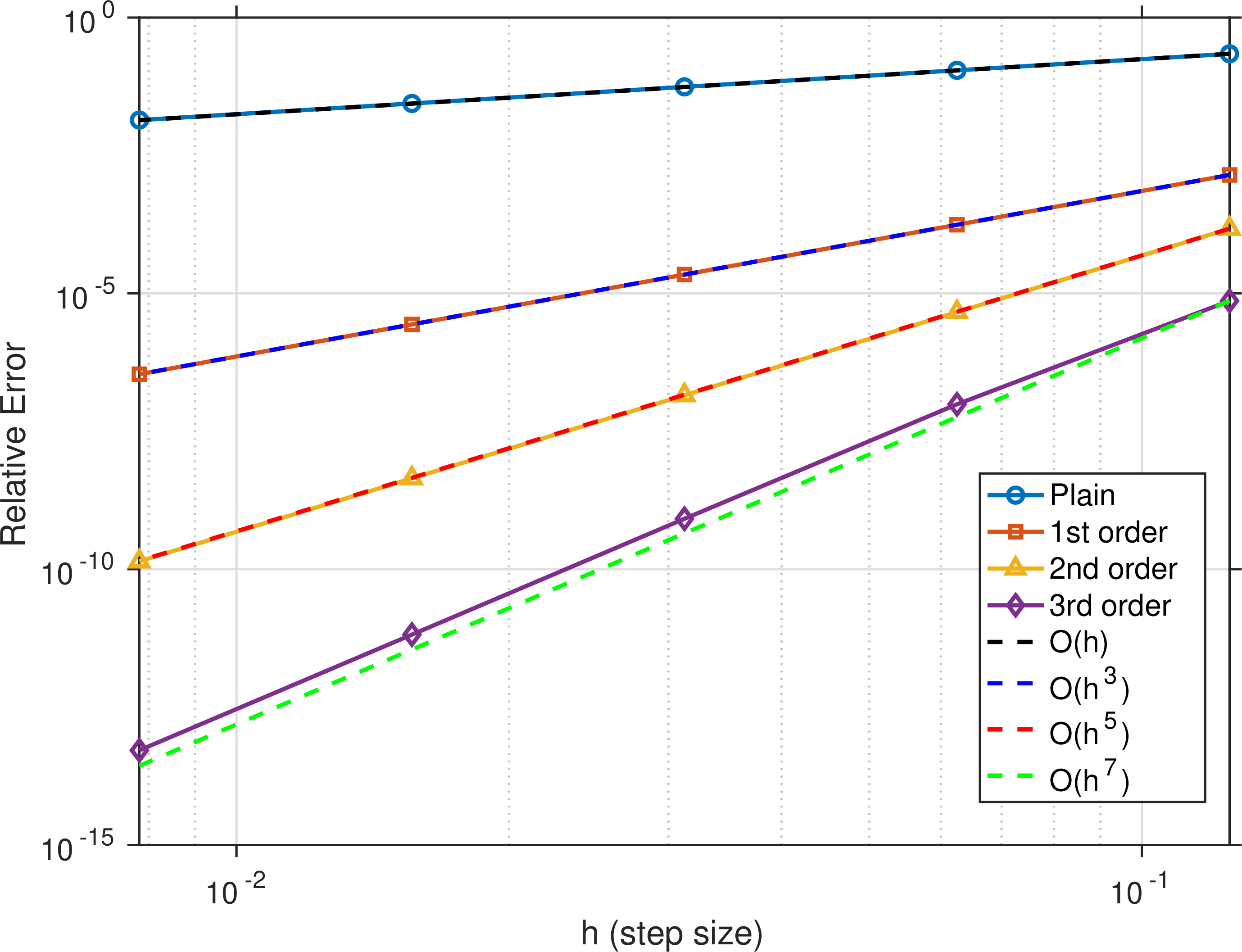
Figure 4: Convergence rates for SinCoTrap with (left) isotropic and (right) anisotropic singular kernels, demonstrating the expected \(O(h^{2p+3})\) scaling for \(p=0,1,2\) (here \(d=3\), \(s=2\)). In the legends, “1st order,” “2nd order,” and “3rd order” refer to the correction levels \(p=0,1,2\), respectively..
The right panel of 4 confirms the predicted convergence rates \(O(h^3)\), \(O(h^5)\), and \(O(h^7)\) for \(p=0,1,2\), respectively, whereas the uncorrected rule is only first-order accurate. Thus, in the anisotropic setting, SinCoTrap retains its designed high-order convergence using only a few correction weights localized near the singular point.
6 Conclusion and discussion↩︎
In this paper, we have developed a locally singularity corrected trapezoidal rule (SinCoTrap) for evaluating singular integrals in arbitrary dimensions, with rigorous theoretical analysis and an efficient computational scheme. Our method preserves the simplicity of the standard trapezoidal rule while achieving high-order accuracy through local corrections applied in a small neighborhood of the singularity. Both theoretical proofs and numerical experiments confirm the scheme’s effectiveness, demonstrating significantly improved convergence rates. A key insight of this work is the connection between the correction weights and generalized zeta functions, which elucidates the underlying mathematical structure of the method.
While our analysis assumes the integrand is either compactly supported or periodic, the quadrature rule can be applied to more general functions. In such cases, to maintain high-order accuracy, it must be combined with a boundary correction scheme [4], [18] for the trapezoidal rule.
Several directions for future research emerge from this work. First, extension to more general singular kernels beyond the power-law form \(1/|\boldsymbol{x}|^s\) would broaden the applicability of the method. Second, investigation of optimal stencil shapes and sizes for specific applications could further improve computational efficiency. Third, generalization to nearly singular integrals, where the singularity is close to but not within the integration domain, presents an interesting challenge. Finally, exploring applications in various scientific and engineering fields, such as computational chemistry, fluid dynamics and electromagnetics, could demonstrate the practical utility of the proposed quadrature scheme.
Appendices↩︎
This appendix contains the proofs and technical derivations deferred from the main text, including the convergence order analysis, proofs of the nonsingularity of the moment-matching matrices, properties of the right-hand sides of the moment-matching system, and a discussion of the generalized zeta functions.
7 Preliminaries for the Appendix↩︎
For reference, we fix the Fourier transform convention \[\mathcal{F}[f](\boldsymbol{\xi}) = \widehat{f}(\boldsymbol{\xi}) := \int_{\mathbb{R}^d} f(\boldsymbol{x})\, \mathrm{e}^{-2\pi\imath\,\boldsymbol{x}\cdot \boldsymbol{\xi}}\, \mathrm{d}\boldsymbol{x}.\] We will repeatedly use the Poisson summation formula, which connects lattice sums with Fourier series and is central to both the error analysis and the analytic continuation of the zeta functions.
Lemma 9 (Poisson summation [24]). Let \(f\) be a function in Schwartz space \(\mathcal{S}(\mathbb{R}^d)\). Then we have \[\sum_{\boldsymbol{i}\in \mathbb{Z}^d} f(\boldsymbol{i}) = \sum_{\boldsymbol{k}\in \mathbb{Z}^d} \widehat{f}(\boldsymbol{k}).\]
8 Proofs for convergence order analysis↩︎
Lemma 10. Given \(n\in\mathbb{N}_+\), define the \(\ell_\infty\)-shell \(S_n := \{\boldsymbol{k}\in\mathbb{Z}^d : | \boldsymbol{k} |_\infty=n\}\). Then the number of lattice points in \(S_n\) is 4 \[\#S_n = (2n+1)^d-(2n-1)^d \le 2d\,3^{d-1}\,n^{d-1}.\]
Proof. The number of lattice points \(\#S_n\) is the difference of number of lattice points in nested cubes, i.e., \[\#\{\boldsymbol{k}\in\mathbb{Z}^d:| \boldsymbol{k} |_\infty\le n\}=(2n+1)^d, \quad \#\{\boldsymbol{k}\in\mathbb{Z}^d:| \boldsymbol{k} |_\infty\le n-1\}=(2n-1)^d.\] For the upper bound, apply the mean value theorem to \(f(x)=x^d\) on the interval \((2n-1,2n+1)\), then there exists \(\xi\in(2n-1,2n+1)\) such that \[(2n+1)^d-(2n-1)^d = 2 f'(\xi) = 2d\,\xi^{d-1} \leq 2d(2n+1)^{d-1} \leq 2d\,3^{d-1}\,n^{d-1}.\] ◻
Lemma 11. For \(q\in \mathbb{N}\), \(s\in \mathbb{C}\setminus \{0\}\), \(\boldsymbol{\alpha}\in \mathbb{N}^d\) and \(0 \neq \boldsymbol{x}= (x_1, \ldots, x_d) \in \mathbb{R}^d\), we have \[\frac{\partial^q}{\partial x_j^q} \left( \frac{\boldsymbol{x}^{2\boldsymbol{\alpha}}}{|\boldsymbol{x}|^s} \right) = \frac{1}{|\boldsymbol{x}|^{q+s-2| \boldsymbol{\alpha} |_1}} P_{q, \boldsymbol{\alpha},j}\left( \frac{\boldsymbol{x}}{|\boldsymbol{x}|} \right), \quad j=1, \ldots, d,\] where \(P_{q, \boldsymbol{\alpha},j}(\boldsymbol{x})\) is a polynomial with degree \(\mathrm{deg} P_{q, \boldsymbol{\alpha},j} \leq q + 2| \boldsymbol{\alpha} |_1\) in variable \(\boldsymbol{x}\). Furthermore, the coefficients of \(P_{q, \boldsymbol{\alpha},j}(\boldsymbol{x})\) depend polynomially on the parameter \(s\).
Proof. Since \(|\boldsymbol{x}|>0\), for complex \(s\) we have \(|\boldsymbol{x}|^{-s}:=\exp(-s\log|\boldsymbol{x}|)\), where \(\log|\boldsymbol{x}|\) is real, so no choice of complex logarithm branch is involved. Differentiation with respect to the real variable \(x_j\) therefore gives \[\frac{\partial}{\partial x_j}|\boldsymbol{x}|^{-s} =-s x_j|\boldsymbol{x}|^{-s-2},\] which is the same formula as for real \(s\).
We complete the proof by induction on \(q\). For \(q=0\), \[\frac{\boldsymbol{x}^{2\boldsymbol{\alpha}}}{|\boldsymbol{x}|^s} = \frac{1}{|\boldsymbol{x}|^{s-2| \boldsymbol{\alpha} |_1}} \left( \frac{\boldsymbol{x}}{|\boldsymbol{x}|} \right)^{2\boldsymbol{\alpha}}, \quad P_{0, \boldsymbol{\alpha},j} (\boldsymbol{x}) = \boldsymbol{x}^{2\boldsymbol{\alpha}}.\] For the inductive step, we assume the result holds for \(q\) and differentiate again: \[\begin{align} \frac{\partial^{q+1}}{\partial x_j^{q+1}} \left( \frac{\boldsymbol{x}^{2\boldsymbol{\alpha}}}{|\boldsymbol{x}|^s} \right) &= \frac{\partial}{\partial x_j} \left( \frac{1}{|\boldsymbol{x}|^{s + q - 2| \boldsymbol{\alpha} |_1}} P_{q, \boldsymbol{\alpha},j}\left( \frac{\boldsymbol{x}}{|\boldsymbol{x}|} \right) \right) \\ &= \frac{-(s + q - 2| \boldsymbol{\alpha} |_1)}{|\boldsymbol{x}|^{s + q - 2| \boldsymbol{\alpha} |_1 + 1}} \, \frac{x_j}{|\boldsymbol{x}|} \, P_{q, \boldsymbol{\alpha},j}\left( \frac{\boldsymbol{x}}{|\boldsymbol{x}|} \right) \\ &\quad + \frac{1}{|\boldsymbol{x}|^{s + q - 2| \boldsymbol{\alpha} |_1}} \left[ P^{(j)}_{q, \boldsymbol{\alpha},j}\left(\frac{\boldsymbol{x}}{|\boldsymbol{x}|}\right) \left(\frac{1}{|\boldsymbol{x}|} - \frac{x_j^2}{|\boldsymbol{x}|^3} \right) - \sum_{l\neq j} P^{(l)}_{q, \boldsymbol{\alpha},j}\left(\frac{\boldsymbol{x}}{|\boldsymbol{x}|}\right) \frac{x_jx_l}{|\boldsymbol{x}|^3} \right] \\ &:= \frac{1}{|\boldsymbol{x}|^{s + q + 1 - 2| \boldsymbol{\alpha} |_1}} P_{q+1, \boldsymbol{\alpha},j}\left( \frac{\boldsymbol{x}}{|\boldsymbol{x}|} \right), \end{align}\] where \(P^{(l)}_{q,\boldsymbol{\alpha},j}(\boldsymbol{x})=\frac{\partial}{\partial x_l} P_{q,\boldsymbol{\alpha},j}(\boldsymbol{x})\) for \(l=1, \ldots,d\) are polynomials with \(\deg P^{(l)}_{q,\boldsymbol{\alpha},j} \leq \deg P_{q,\boldsymbol{\alpha},j} - 1\), and \[P_{q+1, \boldsymbol{\alpha},j}(\boldsymbol{x}) := -(s + q - 2| \boldsymbol{\alpha} |_1) x_j P_{q, \boldsymbol{\alpha},j}\left(\boldsymbol{x}\right) + P^{(j)}_{q, \boldsymbol{\alpha},j}\left(\boldsymbol{x}\right)\left(1 - x_j^2\right) - \sum_{l\neq j} P^{(l)}_{q, \boldsymbol{\alpha},j}\left(\boldsymbol{x}\right) x_j x_l\] is a polynomial with degree at most \(q + 2| \boldsymbol{\alpha} |_1 + 1\) in variable \(\boldsymbol{x}= (x_1, \ldots, x_d)\). ◻
Proof of 2. We begin by introducing a smooth cutoff function \(\eta(\boldsymbol{x}) \in C^{\infty}(\mathbb{R}^d)\) such that \[\label{eq:cutoff95rhs} \eta(\boldsymbol{x}) = \eta(|\boldsymbol{x}|), \quad \eta(\boldsymbol{x}) = \begin{cases} 0, & |\boldsymbol{x}| \leq \frac{1}{2}, \\ 1, & |\boldsymbol{x}| \geq 1. \end{cases}\tag{17}\] Then we rewrite the difference of the integral and summation as: \[\begin{align} & \quad \int_{\mathbb{R}^d} g(\boldsymbol{x}h) \frac{\boldsymbol{x}^{2\boldsymbol{\alpha}}}{|\boldsymbol{x}|^s} \,\mathrm{d}\boldsymbol{x} - \sum_{| \boldsymbol{i} |_\infty=1}^{\infty} g(\boldsymbol{i}h) \frac{\boldsymbol{i}^{2\boldsymbol{\alpha}}}{|\boldsymbol{i}|^s} \\ &= \int_{|\boldsymbol{x}| \leq 1} g(\boldsymbol{x}h) \frac{\boldsymbol{x}^{2\boldsymbol{\alpha}}}{|\boldsymbol{x}|^s} (1 - \eta(\boldsymbol{x})) \,\mathrm{d}\boldsymbol{x} + \left( \int_{\mathbb{R}^d} g(\boldsymbol{x}h) \frac{\boldsymbol{x}^{2\boldsymbol{\alpha}}}{|\boldsymbol{x}|^s} \eta(\boldsymbol{x}) \,\mathrm{d}\boldsymbol{x} - \sum_{| \boldsymbol{i} |_\infty=1}^{\infty} g(\boldsymbol{i}h) \frac{\boldsymbol{i}^{2\boldsymbol{\alpha}}}{|\boldsymbol{i}|^s} \eta(\boldsymbol{i}) \right) \\ &:= {\rm I} + {\rm II}. \end{align}\]
8.0.0.1 Estimate of \({\rm I}\).
Note that \(\partial^{\boldsymbol{\beta}} g(0) = 0\) for \(1 \leq | \boldsymbol{\beta} |_1 \leq 2p+1\). Moreover, for multi-index \(| \boldsymbol{\beta} |_1=2p+2\) and constant \(\theta \in [0, 1]\), \[\int_{|\boldsymbol{x}| \leq 1} \Big| \frac{\partial^{\boldsymbol{\beta}} g(\theta \boldsymbol{x}h)}{\boldsymbol{\beta}!} (\boldsymbol{x}h)^{\boldsymbol{\beta}} \frac{\boldsymbol{x}^{2\boldsymbol{\alpha}}}{|\boldsymbol{x}|^s} (1 - \eta(\boldsymbol{x})) \Big| \,\mathrm{d}\boldsymbol{x} \leq C h^{2p+2} \int_{|\boldsymbol{x}|\leq 1} |\boldsymbol{x}|^{2| \boldsymbol{\alpha} |_1 + 2p + 2 - \mathrm{Re}(s)} \,\mathrm{d}\boldsymbol{x} \leq C h^{2p+2},\] where \(0 < \mathrm{Re}(s) < d + 2| \boldsymbol{\alpha} |_1\) guarantees the convergence of the integral. Thus, the Taylor expansion of \(g(\boldsymbol{x} h)\) around \(\boldsymbol{x}=0\) gives \[{\rm I} = \int_{|\boldsymbol{x}| \leq 1} g(\boldsymbol{x}h) \frac{\boldsymbol{x}^{2\boldsymbol{\alpha}}}{|\boldsymbol{x}|^s} (1 - \eta(\boldsymbol{x})) \,\mathrm{d}\boldsymbol{x} = g(0) \int_{|\boldsymbol{x}|\leq 1} \frac{\boldsymbol{x}^{2\boldsymbol{\alpha}}}{|\boldsymbol{x}|^s} (1 - \eta(\boldsymbol{x})) \,\mathrm{d}\boldsymbol{x}+ O(h^{2p+2}).\]
8.0.0.2 Estimate of \({\rm II}\).
Define \[\label{eq:def95fh95rhs} f_h(\boldsymbol{x}) := g(\boldsymbol{x}h) \frac{\boldsymbol{x}^{2\boldsymbol{\alpha}}}{|\boldsymbol{x}|^s} \eta(\boldsymbol{x}),\tag{18}\] then \(f_h(0)=0\) and \(f_h \in C_c^{\infty}(\mathbb{R}^d)\) for \(h > 0\). Apply the Poisson summation formula in 9 we obtain \[\begin{align} {\rm II} = \int_{\mathbb{R}^d} f_h(\boldsymbol{x}) \,\mathrm{d}\boldsymbol{x}- \sum_{| \boldsymbol{i} |_\infty=1}^{\infty} f_h(\boldsymbol{i}) = \widehat{f_h}(0) - \sum_{| \boldsymbol{i} |_\infty=0}^{\infty} f_h(\boldsymbol{i}) = \widehat{f_h}(0) - \sum_{| \boldsymbol{k} |_\infty=0}^{\infty} \widehat{f_h}(\boldsymbol{k}) = - \sum_{| \boldsymbol{k} |_\infty=1}^{\infty} \widehat{f_h}(\boldsymbol{k}). \end{align}\]
Choose integer \[q = 2p+3+d+2| \boldsymbol{\alpha} |_1.\] For each \(\boldsymbol{k}\in \mathbb{Z}^d \setminus \{0\}\), let index \(j = j(\boldsymbol{k}) \in \text{argmax}_{\ell=1, \ldots, d} |k_{\ell}|\) and hence \(|k_j| = | \boldsymbol{k} |_\infty\). Then we have the following Fourier estimate for \(h>0\) sufficiently small, proved in 12 below: \[\widehat{f_h}(\boldsymbol{k}) = g(0)\frac{W(\boldsymbol{k})}{(2\pi k_j)^q} + R_h(\boldsymbol{k}), \qquad |R_h(\boldsymbol{k})|\le C h^{2p+2} \frac{1}{|k_j|^q}, \qquad |W(\boldsymbol{k})|\le C.\] Furthermore, for \(n\in \mathbb{N}_+\), let \(S_n := \{\boldsymbol{k}\in \mathbb{Z}^d : | \boldsymbol{k} |_\infty = n\}\), by 10 the number of elements in \(S_n\) satisfies \(\# S_n \leq C_d n^{d-1}\) for some constant \(C_d>0\) depending only on the dimension \(d\). Thus, whenever \(q > d\), we have \[\sum_{| \boldsymbol{k} |_\infty=1}^{\infty} \frac{1}{|k_j|^q} = \sum_{n=1}^{\infty} \sum_{\boldsymbol{k}\in S_n} \frac{1}{n^q} \leq C_d \sum_{n=1}^{\infty} \frac{1}{n^{q-d+1}} < \infty.\] Therefore, \[{\rm II} = - \sum_{| \boldsymbol{k} |_\infty=1}^{\infty} \widehat{f_h}(\boldsymbol{k}) = - g(0) \sum_{| \boldsymbol{k} |_\infty=1}^{\infty} \frac{W(\boldsymbol{k})}{(2\pi k_j)^q} + O(h^{2p+2}).\]
8.0.0.3 Conclusion.
Combining the estimates for \({\rm I}\) and \({\rm II}\) yields \[{\rm I} + {\rm II} = g(0)b_{\boldsymbol{\alpha}}(s) + O(h^{2p+2}), \quad b_{\boldsymbol{\alpha}}(s) := \int_{|\boldsymbol{x}|\le 1}\frac{\boldsymbol{x}^{2\boldsymbol{\alpha}}}{|\boldsymbol{x}|^s}(1-\eta(\boldsymbol{x}))\,\mathrm{d}\boldsymbol{x} - \sum_{| \boldsymbol{k} |_\infty=1}^{\infty} \frac{W(\boldsymbol{k})}{(2\pi k_j)^q}.\] ◻
Lemma 12. Let \(p\in\mathbb{N}\), \(\boldsymbol{\alpha}\in\mathbb{N}^d\) with \(0\leq| \boldsymbol{\alpha} |_1\leq p\), and \(s\in\mathbb{C}\) with \(0<\mathrm{Re}(s)<d+2| \boldsymbol{\alpha} |_1\). Assume that \(g\in C_c^{\infty}(\mathbb{R}^d)\) satisfies \[\partial^{\boldsymbol{\beta}}g(0)=0, \qquad 1\leq| \boldsymbol{\beta} |_1\leq 2p+1.\] Let \(\eta\) be the cutoff function defined in 17 , and let \(q\in\mathbb{N}\) satisfy \(q\geq 2p+3+d+2| \boldsymbol{\alpha} |_1\). For each \(\boldsymbol{k}\in\mathbb{Z}^d\setminus\{0\}\), choose any index \(j=j(\boldsymbol{k})\) in \(\text{argmax}_{\ell=1,\ldots,d}|k_\ell|\), so that \(|k_j|=| \boldsymbol{k} |_\infty\), and define \[W(\boldsymbol{k}) := (-\imath)^q \int_{\mathbb{R}^d} \partial^q_j \left( \frac{\boldsymbol{x}^{2\boldsymbol{\alpha}}}{|\boldsymbol{x}|^s} \eta(\boldsymbol{x}) \right) \mathrm{e}^{-2\pi \imath\, \boldsymbol{k}\cdot \boldsymbol{x}} \,\mathrm{d}\boldsymbol{x}.\] Then there exists a constant \(C>0\), independent of \(h\) and \(\boldsymbol{k}\), such that \(|W(\boldsymbol{k})|\leq C\) and, for all sufficiently small \(h>0\), the function \(f_h\) defined in 18 satisfies \[\widehat{f_h}(\boldsymbol{k}) = g(0)\frac{W(\boldsymbol{k})}{(2\pi k_j)^q} + R_h(\boldsymbol{k}), \qquad |R_h(\boldsymbol{k})|\le C h^{2p+2} \, \frac{1}{|k_j|^q}.\]
Proof. Since \(f_h\in C_c^{\infty}(\mathbb{R}^d)\), after integration by parts \(q\) times in the \(x_j\) variable we have \[\widehat{f_h}(\boldsymbol{k}) = \int_{\mathbb{R}^d} f_h(\boldsymbol{x})\, \mathrm{e}^{-2\pi \imath\, \boldsymbol{k}\cdot \boldsymbol{x}} \,\mathrm{d}\boldsymbol{x} = \left( \frac{1}{2\pi \imath k_j} \right)^q \int_{\mathbb{R}^d} \partial^q_j \left( g(\boldsymbol{x}h) \frac{\boldsymbol{x}^{2\boldsymbol{\alpha}}}{|\boldsymbol{x}|^s} \eta(\boldsymbol{x}) \right) \mathrm{e}^{-2\pi \imath\, \boldsymbol{k}\cdot \boldsymbol{x}} \,\mathrm{d}\boldsymbol{x}.\]
8.0.0.4 Bound of \(W(\boldsymbol{k})\).
By definition of \(W(\boldsymbol{k})\), note that \(\eta(\boldsymbol{x})=0\) for \(|\boldsymbol{x}|\leq \frac{1}{2}\) and \(\eta(\boldsymbol{x})=1\) for \(|\boldsymbol{x}|\geq 1\), we have \[|W(\boldsymbol{k})| \leq \int_{\mathbb{R}^d}\left|\partial_j^q\!\left(\frac{\boldsymbol{x}^{2\boldsymbol{\alpha}}}{|\boldsymbol{x}|^s}\eta(\boldsymbol{x})\right)\right|\,\mathrm{d}\boldsymbol{x} \leq \int_{\frac{1}{2} \leq |\boldsymbol{x}| \leq 1} \left|\partial_j^q\!\left(\frac{\boldsymbol{x}^{2\boldsymbol{\alpha}}}{|\boldsymbol{x}|^s}\eta(\boldsymbol{x})\right)\right|\,\mathrm{d}\boldsymbol{x} + \int_{|\boldsymbol{x}| \geq 1} \left|\partial_j^q\!\left(\frac{\boldsymbol{x}^{2\boldsymbol{\alpha}}}{|\boldsymbol{x}|^s}\right)\right|\,\mathrm{d}\boldsymbol{x}.\] On the annulus \(\{\frac{1}{2}\leq|\boldsymbol{x}|\leq1\}\), the integrand is smooth and hence integrable. For \(|\boldsymbol{x}|\geq1\), 11 and the boundedness of \(P_{q,\boldsymbol{\alpha},j}\) on the unit sphere imply \[\left|\partial_j^q\!\left(\frac{\boldsymbol{x}^{2\boldsymbol{\alpha}}}{|\boldsymbol{x}|^s}\right)\right| \leq C|\boldsymbol{x}|^{-q-\mathrm{Re}(s)+2| \boldsymbol{\alpha} |_1}, \qquad |\boldsymbol{x}|\geq1.\] Here \(C\) is chosen independently of \(j\), since \(j\in\{1,\ldots,d\}\). Consequently, \[\int_{|\boldsymbol{x}|\geq1} \left|\partial_j^q\!\left(\frac{\boldsymbol{x}^{2\boldsymbol{\alpha}}}{|\boldsymbol{x}|^s}\right)\right|\,\mathrm{d}\boldsymbol{x} \leq C\int_1^\infty r^{-q-\mathrm{Re}(s)+2| \boldsymbol{\alpha} |_1+d-1}\,\mathrm{d}r<\infty,\] because \(q+\mathrm{Re}(s)>d+2| \boldsymbol{\alpha} |_1\). Thus we have \(|W(\boldsymbol{k})|\leq C\).
8.0.0.5 Estimate of the remainder \(R_h(\boldsymbol{k})\).
Define \[\Delta_h(\boldsymbol{x}):=\bigl(g(h\boldsymbol{x})-g(0)\bigr)\eta(\boldsymbol{x})\frac{\boldsymbol{x}^{2\boldsymbol{\alpha}}}{|\boldsymbol{x}|^s}.\] Then \[\widehat{f_h}(\boldsymbol{k}) - g(0)\frac{W(\boldsymbol{k})}{(2\pi k_j)^q} = \left(\frac{1}{2\pi \imath k_j}\right)^q \int_{\mathbb{R}^d} \partial_j^q \Delta_h(\boldsymbol{x})\,\mathrm{e}^{-2\pi \imath\boldsymbol{k}\cdot \boldsymbol{x}}\,\mathrm{d}\boldsymbol{x} =: R_h(\boldsymbol{k}),\] and hence \[|R_h(\boldsymbol{k})| \le (2\pi)^{-q}|k_j|^{-q}\,\|\partial_j^q\Delta_h\|_{L^1(\mathbb{R}^d)}.\] It remains to show \(\|\partial_j^q\Delta_h\|_{L^1(\mathbb{R}^d)}\le Ch^{2p+2}\). Since \(\eta(\boldsymbol{x})=0\) for \(|\boldsymbol{x}|\le 1/2\), we only integrate over \(|\boldsymbol{x}|\ge 1/2\). Furthermore, fix \(R>0\) such that \(\operatorname{supp}(g(\boldsymbol{x}))\subset\{\boldsymbol{x}:|\boldsymbol{x}| < R\}\), so \(\operatorname{supp}(g(h\boldsymbol{x}))\subset\{\boldsymbol{x}:|\boldsymbol{x}| < R/h\}\).
By Leibniz’ rule, \[\partial_j^q \Delta_h(\boldsymbol{x}) = \sum_{m=0}^{q}\binom{q}{m}\, \partial_j^{m}\bigl(g(h\boldsymbol{x})-g(0)\bigr)\, \partial_j^{\,q-m}\!\left(\eta(\boldsymbol{x})\frac{\boldsymbol{x}^{2\boldsymbol{\alpha}}}{|\boldsymbol{x}|^s}\right).\] We prove \(\|\partial_j^q\Delta_h\|_{L^1(\mathbb{R}^d)}\le Ch^{2p+2}\) in three steps. We first give bounds for \(\partial_j^{m}(g(h\boldsymbol{x})-g(0))\) and \(\partial_j^{q-m}\!\left(\eta(\boldsymbol{x})\boldsymbol{x}^{2\boldsymbol{\alpha}}/|\boldsymbol{x}|^s\right)\), then combine these bounds to obtain the \(L^1\) estimate of \(\partial_j^q\Delta_h\).
8.0.0.6 Step 1: bounds for \(\partial_j^{m}(g(h\boldsymbol{x})-g(0))\).
Let \(m\in\{0,1,\ldots,q\}\). Since \(\partial^{\boldsymbol{\beta}}g(0)=0\) for \(1\le | \boldsymbol{\beta} |_1\le 2p+1\), Taylor’s theorem gives, for \(m=0\), we have \(|g(h\boldsymbol{x})-g(0)| \le C (h|\boldsymbol{x}|)^{2p+2}\); for \(m=1,\ldots,2p+1\), we have \[\left|\partial_j^m\bigl(g(h\boldsymbol{x})-g(0)\bigr)\right| = h^m |(\partial_j^m g)(h\boldsymbol{x}) - (\partial_j^m g)(0)| \le C h^m (h|\boldsymbol{x}|)^{2p+2-m} = C h^{2p+2}|\boldsymbol{x}|^{2p+2-m}.\] Further, for \(2p+2 \leq m \leq q\), the uniform boundedness of \(\partial_j^m g\) and the chain rule give \[\left|\partial_j^m\bigl(g(h\boldsymbol{x})-g(0)\bigr)\right| =h^m|(\partial_j^m g)(h\boldsymbol{x})|\leq Ch^m.\] Note that on the region \(\{|\boldsymbol{x}|\le R/h\}\), \(h|\boldsymbol{x}| \leq R\) implies \[h^m = h^{2p+2}(h|\boldsymbol{x}|)^{m-(2p+2)}|\boldsymbol{x}|^{2p+2-m} \le C_R h^{2p+2}|\boldsymbol{x}|^{2p+2-m}.\] Therefore, we conclude that for all \(m=0,1,\ldots,q\), \[\left|\partial_j^{m}\bigl(g(h\boldsymbol{x})-g(0)\bigr)\right| \le C h^{2p+2}|\boldsymbol{x}|^{2p+2-m}, \qquad \frac{1}{2}\le |\boldsymbol{x}|\le R/h.\]
8.0.0.7 Step 2: bounds for \(\partial_j^{q-m}\!\left(\eta(\boldsymbol{x})\boldsymbol{x}^{2\boldsymbol{\alpha}}/|\boldsymbol{x}|^s\right)\).
For \(|\boldsymbol{x}|\ge 1\), we have \(\eta(\boldsymbol{x})=1\) and thus 11, together with the boundedness of \(P_{q-m,\boldsymbol{\alpha},j}\) on the unit sphere, gives \[\left|\partial_j^{\,q-m}\!\left(\eta(\boldsymbol{x})\frac{\boldsymbol{x}^{2\boldsymbol{\alpha}}}{|\boldsymbol{x}|^s}\right)\right| = \left|\partial_j^{\,q-m}\!\left(\frac{\boldsymbol{x}^{2\boldsymbol{\alpha}}}{|\boldsymbol{x}|^s}\right)\right| \le C |\boldsymbol{x}|^{2| \boldsymbol{\alpha} |_1-\mathrm{Re}(s)-(q-m)},\qquad |\boldsymbol{x}|\ge 1,\] where \(C\) is chosen uniformly for \(m\in\{0,\ldots,q\}\) and \(j\in\{1,\ldots,d\}\). On the annulus \(\{1/2\le |\boldsymbol{x}|\le 1\}\), the function \(\eta(\boldsymbol{x})\boldsymbol{x}^{2\boldsymbol{\alpha}}/|\boldsymbol{x}|^s\) is smooth and the integral domain is bounded, hence \[\left|\partial_j^{\,q-m}\!\left(\eta(\boldsymbol{x})\frac{\boldsymbol{x}^{2\boldsymbol{\alpha}}}{|\boldsymbol{x}|^s}\right)\right| \leq C \leq C |\boldsymbol{x}|^{2| \boldsymbol{\alpha} |_1-\mathrm{Re}(s)-(q-m)}, \qquad \frac{1}{2}\le |\boldsymbol{x}|\le 1.\] Therefore, we obtain the uniform bound for \(\partial_j^{q-m}\!\left(\eta(\boldsymbol{x})\boldsymbol{x}^{2\boldsymbol{\alpha}}/|\boldsymbol{x}|^s\right)\) over \(|\boldsymbol{x}|\ge 1/2\).
8.0.0.8 Step 3: \(L^1\) estimate of \(\partial_j^q\Delta_h\).
For \(h > 0\) sufficiently small, we have \(R/h > 1\). Using Steps 1, 2 and splitting \(\mathbb{R}^d\) into \(\{\frac{1}{2} \leq |\boldsymbol{x}|\leq R/h\}\) and \(\{|\boldsymbol{x}| \geq R/h\}\), we obtain \[\begin{align} \left\| \partial^q_j \Delta_h \right\|_{L^1(\mathbb{R}^d)} = \left( \int_{\frac{1}{2} \leq |\boldsymbol{x}| \leq R/h} + \int_{|\boldsymbol{x}| \geq R/h} \right) \left| \partial^q_j \Delta_h(\boldsymbol{x}) \right| \mathrm{d}\boldsymbol{x} := T_1 + T_2. \end{align}\] For the first part, we have \[\begin{align} T_{1} &= \int_{\frac{1}{2} \leq |\boldsymbol{x}| \leq R/h} \Big| \sum_{m=0}^q \binom{q}{m}\, \partial_j^{m}\bigl(g(h\boldsymbol{x})-g(0)\bigr)\, \partial_j^{\,q-m}\!\left(\eta(\boldsymbol{x})\frac{\boldsymbol{x}^{2\boldsymbol{\alpha}}}{|\boldsymbol{x}|^s}\right) \Big| \, \mathrm{d}\boldsymbol{x}\\ &\le C h^{2p+2}\sum_{m=0}^{q}\binom{q}{m} \int_{\frac{1}{2} \le |\boldsymbol{x}|\le R/h} |\boldsymbol{x}|^{2p+2-m}\,|\boldsymbol{x}|^{2| \boldsymbol{\alpha} |_1-\mathrm{Re}(s)-(q-m)} \mathrm{d}\boldsymbol{x}\\ &\le C h^{2p+2} \int_{\frac{1}{2}}^{R/h} r^{2p+2+2| \boldsymbol{\alpha} |_1-\mathrm{Re}(s)-q+d-1}\,\mathrm{d}r \le C h^{2p+2}, \end{align}\] where the last inequality uses \(q\ge 2p+3+d+2| \boldsymbol{\alpha} |_1\), so the exponent of \(r\) is at most \(-2-\mathrm{Re}(s)<-2\).
For \(T_2\), note that \(g(h\boldsymbol{x})=0\) when \(|\boldsymbol{x}|\ge R/h\), hence \(\Delta_h(\boldsymbol{x})=-g(0)\eta(\boldsymbol{x})\boldsymbol{x}^{2\boldsymbol{\alpha}}/|\boldsymbol{x}|^s\) there, and since \(\eta(\boldsymbol{x})=1\) for \(|\boldsymbol{x}|\ge 1\) and \(R/h > 1\) for \(h>0\) sufficiently small, \[T_2 = |g(0)| \int_{|\boldsymbol{x}|\ge R/h}\left|\partial_j^q\left(\frac{\boldsymbol{x}^{2\boldsymbol{\alpha}}}{|\boldsymbol{x}|^s}\right)\right|\mathrm{d}\boldsymbol{x} \le C \int_{R/h}^{\infty} r^{-q-\mathrm{Re}(s)+2| \boldsymbol{\alpha} |_1+d-1}\,\mathrm{d}r \le C h^{2p+2}.\] Therefore \(\|\partial_j^q\Delta_h\|_{L^1(\mathbb{R}^d)}\le C h^{2p+2}\), which completes the proof. ◻
9 Proofs of non-singularity of moment-matching matrix↩︎
Proof of 1. Recall that \[A_{jk}=\sum_{\boldsymbol{i}\in\mathcal{G}_{\boldsymbol{\beta}_k}}\boldsymbol{i}^{2\boldsymbol{\alpha}_j}.\] Since the exponents are even, \(\boldsymbol{i}^{2\boldsymbol{\alpha}_j}\) is constant on the sign-orbit \(\mathcal{G}_{\boldsymbol{\beta}_k}\), hence \[A_{jk}=c(\boldsymbol{\beta}_k)\,\boldsymbol{\beta}_k^{2\boldsymbol{\alpha}_j},\qquad c(\boldsymbol{\beta}):=\#\mathcal{G}_{\boldsymbol{\beta}}=2^{r(\boldsymbol{\beta})},\,\, r(\boldsymbol{\beta}):=\#\{\ell:\beta_\ell\neq 0\}.\] Therefore \(A=MD\), where \(D=\mathrm{diag}(c(\boldsymbol{\beta}_k))\) has strictly positive diagonal entries and \[M_{jk}=\boldsymbol{\beta}_k^{2\boldsymbol{\alpha}_j}.\] Since \(D\) is invertible, it suffices to show that \(M\) is nonsingular.
For \(m\in\mathbb{N}\), define the even 1D polynomials \[q_m(x) := \prod_{r=0}^{m-1} (x^2-r^2) = x^2(x^2-1^2)\cdots(x^2-(m-1)^2), \qquad q_0(x):=1.\] and for \(\boldsymbol{\gamma}\in\mathbb{N}^d\) define the tensor-product polynomials \[Q_{\boldsymbol{\gamma}}(\boldsymbol{x}):=\prod_{\ell=1}^d q_{\gamma_\ell}(x_\ell) = \prod_{\ell=1}^d \prod_{r=0}^{\gamma_\ell-1} (x_\ell^2-r^2).\] For \(\boldsymbol{\beta}\in\mathbb{N}^d\), we have \(Q_{\boldsymbol{\gamma}}(\boldsymbol{\beta})=0\) whenever \(\beta_\ell<\gamma_\ell\) for some \(\ell\) (since then the factor with \(r=\beta_\ell\) appears and vanishes). In particular, \[Q_{\boldsymbol{\gamma}}(\boldsymbol{\beta})=0 \quad \text{unless } \boldsymbol{\gamma}\le \boldsymbol{\beta},\] where \(\boldsymbol{\gamma}\le \boldsymbol{\beta}\) means componentwise inequality. Moreover, for \(| \boldsymbol{\beta} |_1 > 0\), \[Q_{\boldsymbol{\beta}}(\boldsymbol{\beta}) =\prod_{\ell=1}^d\prod_{r=0}^{\beta_\ell-1}(\beta_\ell^2-r^2)\neq 0, \quad \text{and} \quad Q_{\boldsymbol{0}}(\boldsymbol{0}) = 1.\] Order the index set \(\{\boldsymbol{\gamma}\in\mathbb{N}^d:0\le | \boldsymbol{\gamma} |_1\le p\}\) by any linear extension of the partial order \(\boldsymbol{\gamma}\le\boldsymbol{\beta}\) (componentwise). Then the evaluation matrix \[E_{\boldsymbol{\gamma},\boldsymbol{\beta}}:=Q_{\boldsymbol{\gamma}}(\boldsymbol{\beta})\] is upper triangular with nonzero diagonal, hence \(E\) is invertible.
Now we express \(Q_{\boldsymbol{\gamma}}(\boldsymbol{x})\) in the monomial basis. Since \(q_m(x)\) is an even polynomial of degree \(2m\) with leading coefficient \(1\), it admits an expansion \[q_m(x)=\sum_{r=0}^{m}l_{m,r}\,x^{2r},\qquad l_{m,m}=1.\] Consequently, for every \(\boldsymbol{\gamma}\in\mathbb{N}^d\) we can expand the tensor product as \[Q_{\boldsymbol{\gamma}}(\boldsymbol{x}) =\prod_{\ell=1}^d\Bigl(\sum_{r=0}^{\gamma_\ell}l_{\gamma_\ell,r}\,x_\ell^{2r}\Bigr) =\sum_{\boldsymbol{\delta}\le \boldsymbol{\gamma}} L_{\boldsymbol{\gamma},\boldsymbol{\delta}}\,\boldsymbol{x}^{2\boldsymbol{\delta}}, \qquad L_{\boldsymbol{\gamma},\boldsymbol{\delta}}:=\prod_{\ell=1}^d l_{\gamma_\ell,\delta_\ell}.\] Specifically, we have \(L_{\boldsymbol{\gamma},\boldsymbol{\gamma}}=1\). Furthermore, we extend this notation by setting \(L_{\boldsymbol{\gamma},\boldsymbol{\delta}}=0\) whenever \(\delta_\ell>\gamma_\ell\) for at least one component \(\ell\). Under the same ordering for \(\{\boldsymbol{\gamma}\in\mathbb{N}^d:0\le | \boldsymbol{\gamma} |_1\le p\}\) as above, the matrix \(L=[L_{\boldsymbol{\gamma},\boldsymbol{\delta}}]\) is lower triangular with ones on the diagonal, hence invertible.
Evaluating the expansion at \(\boldsymbol{x}=\boldsymbol{\beta}\) yields \[Q_{\boldsymbol{\gamma}}(\boldsymbol{\beta})=\sum_{\boldsymbol{\delta}\le \boldsymbol{\gamma}} L_{\boldsymbol{\gamma},\boldsymbol{\delta}}\,\boldsymbol{\beta}^{2\boldsymbol{\delta}}.\] Stacking these identities for all \(\boldsymbol{\gamma},\boldsymbol{\beta}\) gives the matrix relation \[E = L M.\] Since \(E\) and \(L\) are invertible, then \(M\) is invertible. Therefore \(A=MD\) is invertible as well. ◻
10 Proofs for right-hand side of moment-matching system↩︎
We first introduce a lemma to verify the holomorphicity of an integral with respect to a complex parameter.
Lemma 13 (Holomorphic parameter integral). Let \(U\subset \mathbb{R}^d\) be measurable and let \(\Omega\subset \mathbb{C}\) be open. Suppose \(F:\Omega\times U\to \mathbb{C}\) is jointly measurable and satisfies:
For each fixed \(\boldsymbol{x}\in U\), the map \(z\mapsto F(z,\boldsymbol{x})\) is holomorphic on \(\Omega\).
For every compact set \(K\subset \Omega\), there exists \(M_K\in L^1(U)\) such that \(|F(z,\boldsymbol{x})|\le M_K(\boldsymbol{x})\) for all \(z\in K\) and \(\boldsymbol{x}\in U\).
Define \[f(z) := \int_U F(z,\boldsymbol{x})\,\mathrm{d}\boldsymbol{x}, \qquad z\in \Omega.\] Then \(f\) is holomorphic on \(\Omega\).
Proof. By dominated convergence, \(f\) is continuous on \(\Omega\). Let \(T\) be any triangle whose closure \(\overline{T}\) is contained in \(\Omega\). By assumption (2), there exists \(M\in L^1(U)\) such that \(|F(z,\boldsymbol{x})|\leq M(\boldsymbol{x})\) for \(z\in\overline{T}\). Hence Fubini’s theorem and Cauchy’s theorem give \[\int_{\partial T}f(z)\,\mathrm{d}z =\int_U\left(\int_{\partial T}F(z,\boldsymbol{x})\,\mathrm{d}z\right)\mathrm{d}\boldsymbol{x} =0.\] Thus \(f\) is holomorphic by Morera’s theorem. ◻
Proof of 4. Recall that in the proof of 2 we obtained \[\begin{align} b_{\boldsymbol{\alpha}}(s) &= \lim_{N\rightarrow \infty} \left( \int_{\mathbb{R}^d} g(\boldsymbol{x}\frac{a}{N}) \frac{\boldsymbol{x}^{2\boldsymbol{\alpha}}}{|\boldsymbol{x}|^s} \mathrm{d}\boldsymbol{x} - \sum_{| \boldsymbol{i} |_\infty=1}^{\infty} g(\boldsymbol{i}\frac{a}{N}) \frac{\boldsymbol{i}^{2\boldsymbol{\alpha}}}{|\boldsymbol{i}|^s} \right) \\ &= \int_{|\boldsymbol{x}|\le 1}\frac{\boldsymbol{x}^{2\boldsymbol{\alpha}}}{|\boldsymbol{x}|^s}(1-\eta(\boldsymbol{x}))\,\mathrm{d}\boldsymbol{x} - \sum_{| \boldsymbol{k} |_\infty=1}^{\infty}\frac{W(\boldsymbol{k};s)}{(2\pi k_j)^q} =: b_{\boldsymbol{\alpha}}^{(1)}(s) - b_{\boldsymbol{\alpha}}^{(2)}(s), \qquad s\in D_1, \end{align}\] where \(j=j(\boldsymbol{k})\in \text{argmax}_{\ell=1, \ldots, d} |k_{\ell}|\) and \(q = 2p+3+d+2| \boldsymbol{\alpha} |_1\) are chosen as in the proof of 2. We show that both \(b_{\boldsymbol{\alpha}}^{(1)}\) and \(b_{\boldsymbol{\alpha}}^{(2)}\) are holomorphic on \(D_1 = \left\{ s \in \mathbb{C}\, : \, 0 < \mathrm{Re}(s) < d+ 2| \boldsymbol{\alpha} |_1 \right\}\).
For the first term \(b_{\boldsymbol{\alpha}}^{(1)}(s)\), we split the integral as \[b_{\boldsymbol{\alpha}}^{(1)}(s) = \int_{\frac{1}{2}\le |\boldsymbol{x}|\le 1}\frac{\boldsymbol{x}^{2\boldsymbol{\alpha}}}{|\boldsymbol{x}|^s}(1-\eta(\boldsymbol{x}))\,\mathrm{d}\boldsymbol{x} + \int_{|\boldsymbol{x}|\le \frac{1}{2}}\frac{\boldsymbol{x}^{2\boldsymbol{\alpha}}}{|\boldsymbol{x}|^s}\,\mathrm{d}\boldsymbol{x} =: J_1(s)+J_2(s).\] For \(J_1\), the integrand is holomorphic in \(s\) for each \(\boldsymbol{x}\) in the integration domain, and is uniformly bounded on compact subsets of \(D_1\). Thus, by 13, \(J_1\) is holomorphic on \(D_1\). For \(J_2\), using polar coordinates \(\boldsymbol{x}=r\omega\) with \(\omega\in\mathbb{S}^{d-1}\), \[\begin{align} J_2(s) = \int_{\mathbb{S}^{d-1}}\omega^{2\boldsymbol{\alpha}}\,\mathrm{d}S(\omega)\int_0^{1/2} r^{2| \boldsymbol{\alpha} |_1-s+d-1}\,\mathrm{d}r = \left(\int_{\mathbb{S}^{d-1}}\omega^{2\boldsymbol{\alpha}}\,\mathrm{d}S(\omega)\right) \frac{2^{\,s-d-2| \boldsymbol{\alpha} |_1}}{d+2| \boldsymbol{\alpha} |_1-s}. \end{align}\] Since \(D_1\) excludes \(s=d+2| \boldsymbol{\alpha} |_1\), the right-hand side is holomorphic on \(D_1\). Hence \(b_{\boldsymbol{\alpha}}^{(1)}\) is holomorphic on \(D_1\).
For the second term \(b_{\boldsymbol{\alpha}}^{(2)}\), fix an arbitrary compact set \(K\subset D_1\) and set \(\sigma_K:=\min_{s\in K}\mathrm{Re}(s)>0\). For each fixed \(\boldsymbol{k}\neq0\), \[\begin{align} W(\boldsymbol{k};s) &= (-\imath)^q \int_{\mathbb{R}^d} \partial_j^q\!\left(\frac{\boldsymbol{x}^{2\boldsymbol{\alpha}}}{|\boldsymbol{x}|^s}\eta(\boldsymbol{x})\right) \mathrm{e}^{-2\pi \imath\, \boldsymbol{k}\cdot \boldsymbol{x}}\,\mathrm{d}\boldsymbol{x}\\ &= (-\imath)^q \int_{\frac{1}{2}\le |\boldsymbol{x}|\le 1}\partial_j^q\!\left(\frac{\boldsymbol{x}^{2\boldsymbol{\alpha}}}{|\boldsymbol{x}|^s}\eta(\boldsymbol{x})\right) \mathrm{e}^{-2\pi \imath\,\boldsymbol{k}\cdot \boldsymbol{x}}\,\mathrm{d}\boldsymbol{x} + (-\imath)^q \int_{|\boldsymbol{x}|\geq 1}\partial_j^q\!\left(\frac{\boldsymbol{x}^{2\boldsymbol{\alpha}}}{|\boldsymbol{x}|^s}\right) \mathrm{e}^{-2\pi \imath\,\boldsymbol{k}\cdot \boldsymbol{x}}\,\mathrm{d}\boldsymbol{x}. \end{align}\] The integrand is holomorphic in \(s\) for each fixed \(\boldsymbol{x}\). On the annulus \(\{1/2\le|\boldsymbol{x}|\le1\}\), it is bounded uniformly for \(s\in K\). On \(\{|\boldsymbol{x}|\ge1\}\), 11 gives, uniformly for \(s\in K\), \[\left|\partial_j^q\!\left(\frac{\boldsymbol{x}^{2\boldsymbol{\alpha}}}{|\boldsymbol{x}|^s}\right)\right| \le C_K|\boldsymbol{x}|^{-q-\mathrm{Re}(s)+2| \boldsymbol{\alpha} |_1} \le C_K|\boldsymbol{x}|^{-q-\sigma_K+2| \boldsymbol{\alpha} |_1}.\] This majorant is integrable because \(q+\sigma_K>d+2| \boldsymbol{\alpha} |_1\). Since \(K\subset D_1\) was arbitrary, 13 shows that \(W(\boldsymbol{k};\cdot)\) is holomorphic on \(D_1\). Moreover, the estimates for the integrands in \(W(\boldsymbol{k};s)\) are uniform in \(\boldsymbol{k}\). Thus, \[\sup_{s\in K}\left|\frac{W(\boldsymbol{k};s)}{(2\pi k_j)^q}\right| \leq \frac{C_K}{|k_j|^q}, \qquad \boldsymbol{k}\in\mathbb{Z}^d\setminus\{0\},\] where \(C_K\) is a constant independent of \(\boldsymbol{k}\). Since \(|k_j|=| \boldsymbol{k} |_\infty\), 10 and \(q>d\) imply \[\sum_{| \boldsymbol{k} |_\infty=1}^{\infty}|k_j|^{-q} \leq C_d\sum_{n=1}^{\infty}n^{d-1-q}<\infty.\] The Weierstrass M-test therefore gives uniform convergence of the series defining \(b_{\boldsymbol{\alpha}}^{(2)}\) on every compact \(K\subset D_1\). By the Weierstrass theorem, \(b_{\boldsymbol{\alpha}}^{(2)}\) is holomorphic on \(D_1\). ◻
Next we give two lemmas analyzing the regular and singular parts of \(b_{\boldsymbol{\alpha}}(s)\) respectively.
Lemma 14. Let \(p \in \mathbb{N}\). Assume that \(g\in C_c^{\infty}(\mathbb{R}^d)\) satisfies \(\operatorname{supp}(g)\subset[-a,a]^d\) and \[g(\boldsymbol{x}) = g(|\boldsymbol{x}|), \qquad \partial^{\boldsymbol{\beta}} g(0) = 0, \quad \text{for } 1 \leq | \boldsymbol{\beta} |_1 \leq 2p+1.\] Given multi-index \(\boldsymbol{\alpha}\in \mathbb{N}^d\) such that \(0 \leq | \boldsymbol{\alpha} |_1 \leq p\), define for \(N\in\mathbb{N}_+\) \[I_N(s) := \int_{\frac{1}{2} \leq | \boldsymbol{x} |_\infty \leq N + \frac{1}{2}} g\!\left(\boldsymbol{x}\frac{a}{N}\right)\frac{\boldsymbol{x}^{2\boldsymbol{\alpha}}}{|\boldsymbol{x}|^s}\,\mathrm{d}\boldsymbol{x} - \sum_{| \boldsymbol{i} |_\infty=1}^{N} g\!\left(\boldsymbol{i}\frac{a}{N}\right)\frac{\boldsymbol{i}^{2\boldsymbol{\alpha}}}{|\boldsymbol{i}|^s}.\] Then for every \(s\) with \(\mathrm{Re}(s) > d+2| \boldsymbol{\alpha} |_1-2\) the limit \[I(s) := \lim_{N\rightarrow\infty} I_N(s)\] exists and defines a holomorphic function on \(D := \{s\in\mathbb{C}:\mathrm{Re}(s) > d+2| \boldsymbol{\alpha} |_1-2\}\).
Proof. We first show \(\{I_N\}\) is locally bounded on domain \(D\) via a shell decomposition and uniform Taylor estimates. This local boundedness, together with pointwise convergence on \(\mathrm{Re}(s) > d+2| \boldsymbol{\alpha} |_1\), implies the limit \(I(s)\) exists and is holomorphic on \(D\) by Vitali-Porter theorem [25].
10.0.0.1 Shell decomposition and local Taylor expansion.
For each \(N\), decompose the integral into shells and shift each shell to the cube \(\{| \boldsymbol{x} |_\infty\le 1/2\}\): \[\begin{align} \int_{\frac{1}{2} \leq | \boldsymbol{x} |_\infty \leq N + \frac{1}{2}} g\!\left(\boldsymbol{x}\frac{a}{N}\right)\frac{\boldsymbol{x}^{2\boldsymbol{\alpha}}}{|\boldsymbol{x}|^s}\,\mathrm{d}\boldsymbol{x} &= \sum_{n=1}^N \int_{n-\frac{1}{2} \leq | \boldsymbol{x} |_\infty \leq n + \frac{1}{2}} g\!\left(\boldsymbol{x}\frac{a}{N}\right)\frac{\boldsymbol{x}^{2\boldsymbol{\alpha}}}{|\boldsymbol{x}|^s}\,\mathrm{d}\boldsymbol{x}\\ &= \sum_{n=1}^N \sum_{| \boldsymbol{i} |_\infty=n} \int_{| \boldsymbol{x} |_\infty\le \frac{1}{2}} g\!\left((\boldsymbol{x}+\boldsymbol{i})\frac{a}{N}\right)\frac{(\boldsymbol{x}+\boldsymbol{i})^{2\boldsymbol{\alpha}}}{|\boldsymbol{x}+\boldsymbol{i}|^s}\,\mathrm{d}\boldsymbol{x}. \end{align}\] Hence we can write \[I_N(s) = \sum_{n=1}^N \delta_{n,N}(s),\] where \[\delta_{n,N}(s) := \sum_{| \boldsymbol{i} |_\infty=n} \int_{| \boldsymbol{x} |_\infty\le \frac{1}{2}} \left[ g\!\left((\boldsymbol{x}+\boldsymbol{i})\frac{a}{N}\right)\frac{(\boldsymbol{x}+\boldsymbol{i})^{2\boldsymbol{\alpha}}}{|\boldsymbol{x}+\boldsymbol{i}|^s} - g\!\left(\boldsymbol{i}\frac{a}{N}\right)\frac{\boldsymbol{i}^{2\boldsymbol{\alpha}}}{|\boldsymbol{i}|^s} \right]\mathrm{d}\boldsymbol{x}.\] For any fixed \(N\), define \[f_{N}(\boldsymbol{x};s) := g\!\left(\boldsymbol{x}\frac{a}{N}\right) \frac{\boldsymbol{x}^{2\boldsymbol{\alpha}}}{|\boldsymbol{x}|^s}.\] Taylor’s theorem with integral remainder gives, for \(| \boldsymbol{x} |_\infty\le 1/2\), \[\label{eq:taylor95bs95regular} f_{N}(\boldsymbol{x}+ \boldsymbol{i};s) - f_{N}(\boldsymbol{i};s) = \sum_{j=1}^d \partial_{x_j} f_{N}(\boldsymbol{i};s)\,x_j + \sum_{j,k=1}^d x_jx_k\int_0^1(1-t) \partial_{x_jx_k}^2f_N(\boldsymbol{i}+t\boldsymbol{x};s)\,\mathrm{d}t.\tag{19}\]
10.0.0.2 Local boundedness of \(\{I_N\}\) on \(D\).
Now we show that \(\{I_N\}\) is uniformly bounded on any compact subset of \(D\). Fix an arbitrary compact set \(K\subset D\) and set \[\sigma_K:=\min_{s\in K}\mathrm{Re}(s)>d+2| \boldsymbol{\alpha} |_1-2.\] According to 11, for \(j, k=1, \ldots, d\), we have \[\frac{\partial f_N}{\partial x_j}(\boldsymbol{x};s) = (\partial_j g)\!\left(\boldsymbol{x}\frac{a}{N}\right) \frac{a}{N} \cdot \frac{\boldsymbol{x}^{2\boldsymbol{\alpha}}}{|\boldsymbol{x}|^s} + g\!\left(\boldsymbol{x}\frac{a}{N}\right) \cdot \frac{1}{|\boldsymbol{x}|^{1+s-2| \boldsymbol{\alpha} |_1}} P_{1, \boldsymbol{\alpha},j}\!\left(\frac{\boldsymbol{x}}{|\boldsymbol{x}|} \right),\] and \[\begin{align} \frac{\partial^2 f_N}{\partial x_j\partial x_k}(\boldsymbol{x};s) &= (\partial_{jk}^2 g)\!\left(\boldsymbol{x}\frac{a}{N}\right) (\frac{a}{N})^2 \cdot \frac{\boldsymbol{x}^{2\boldsymbol{\alpha}}}{|\boldsymbol{x}|^s} \\ &\quad + \frac{a}{N} \frac{1}{|\boldsymbol{x}|^{1+s-2| \boldsymbol{\alpha} |_1}} \left[ (\partial_j g)\!\left(\boldsymbol{x}\frac{a}{N}\right) P_{1, \boldsymbol{\alpha},k}\!\left(\frac{\boldsymbol{x}}{|\boldsymbol{x}|}\right) + (\partial_k g)\!\left(\boldsymbol{x}\frac{a}{N}\right) P_{1, \boldsymbol{\alpha},j}\!\left(\frac{\boldsymbol{x}}{|\boldsymbol{x}|}\right) \right] \\ &\quad - g\!\left(\boldsymbol{x}\frac{a}{N}\right) \cdot \frac{1+s-2| \boldsymbol{\alpha} |_1}{|\boldsymbol{x}|^{2+s-2| \boldsymbol{\alpha} |_1}} \frac{x_k}{|\boldsymbol{x}|} \cdot P_{1, \boldsymbol{\alpha},j}\!\left(\frac{\boldsymbol{x}}{|\boldsymbol{x}|}\right) \\ &\quad + g\!\left(\boldsymbol{x}\frac{a}{N}\right) \cdot \frac{1}{|\boldsymbol{x}|^{2+s-2| \boldsymbol{\alpha} |_1}} \left[ (\partial_kP_{1, \boldsymbol{\alpha},j})\!\left(\frac{\boldsymbol{x}}{|\boldsymbol{x}|}\right) (1 - \frac{x_k^2}{|\boldsymbol{x}|^2}) - \sum_{\ell\neq k} (\partial_\ell P_{1, \boldsymbol{\alpha},j})\!\left(\frac{\boldsymbol{x}}{|\boldsymbol{x}|}\right) \frac{x_{\ell} x_k}{|\boldsymbol{x}|^2} \right], \end{align}\] where \(P_{1, \boldsymbol{\alpha},j}(\boldsymbol{x})\) is a polynomial of \(\boldsymbol{x}\).
Given \(| \boldsymbol{i} |_\infty \leq N\), let \(n=| \boldsymbol{i} |_\infty\), then for \(| \boldsymbol{x} |_\infty\le 1/2\), using \(n \leq N\) it follows that \[\max_{j,k}\sup_{| \boldsymbol{x} |_\infty\le 1/2} \left|\partial^2_{x_jx_k} f_N(\boldsymbol{x}+\boldsymbol{i};s)\right| \le C_K\, n^{2| \boldsymbol{\alpha} |_1-\mathrm{Re}(s)-2} \le C_K\, n^{2| \boldsymbol{\alpha} |_1-\sigma_K-2}.\] Since \(x_j\) is odd and the domain is centrally symmetric, the first order term in 19 integrates to \(0\) over \(\{| \boldsymbol{x} |_\infty\le 1/2\}\). Consequently, the Hessian estimate above gives \[\left|\int_{| \boldsymbol{x} |_\infty\le \frac{1}{2}} \left[f_N(\boldsymbol{i}+\boldsymbol{x};s)-f_N(\boldsymbol{i};s)\right]\,\mathrm{d}\boldsymbol{x}\right| \le C_K\, n^{2| \boldsymbol{\alpha} |_1-\sigma_K-2}.\] Summing over the shell \(\{\boldsymbol{i}\in\mathbb{Z}^d:| \boldsymbol{i} |_\infty=n\}\) and using \(\#\{\boldsymbol{i}:| \boldsymbol{i} |_\infty=n\}\le C_d n^{d-1}\) by 10 gives \[\label{eq:delta95nN95bound} \sup_{s\in K}|\delta_{n,N}(s)| \leq C_K\, n^{d+2| \boldsymbol{\alpha} |_1-\sigma_K-3}, \qquad 1\leq n\leq N.\tag{20}\] Combining \(I_N(s)=\sum_{n=1}^N\delta_{n,N}(s)\) with 20 gives \[\sup_{N\in\mathbb{N}_+}\sup_{s\in K}|I_N(s)| \leq \sum_{n=1}^{\infty} \sup_{N\geq n}\sup_{s\in K}|\delta_{n,N}(s)| \leq C_K\sum_{n=1}^{\infty} n^{d+2| \boldsymbol{\alpha} |_1-\sigma_K-3}<\infty,\] where the last series converges since \(\sigma_K>d+2| \boldsymbol{\alpha} |_1-2\).
10.0.0.3 Holomorphicity of the limit.
For each fixed \(N\), the map \(s\mapsto I_N(s)\) is holomorphic on \(D\) by 13. If \(\mathrm{Re}(s)>d+2| \boldsymbol{\alpha} |_1\), then \(|\boldsymbol{x}|^{2| \boldsymbol{\alpha} |_1-\mathrm{Re}(s)}\) is integrable on \(\{| \boldsymbol{x} |_\infty\geq1/2\}\) and summable over \(\mathbb{Z}^d\setminus\{0\}\). Since \(\operatorname{supp}(g)\subset[-a,a]^d\), we have \(g(a\boldsymbol{i}/N)=0\) whenever \(| \boldsymbol{i} |_\infty>N\). Note that \(g\) is bounded and \(g(a\boldsymbol{x}/N)\to g(0)\) pointwise, dominated convergence with respect to Lebesgue and counting measure gives \[\lim_{N\to\infty}I_N(s) =g(0)\left[ \int_{| \boldsymbol{x} |_\infty\geq1/2}\frac{\boldsymbol{x}^{2\boldsymbol{\alpha}}}{|\boldsymbol{x}|^s}\,\mathrm{d}\boldsymbol{x} -\sum_{| \boldsymbol{i} |_\infty=1}^{\infty} \frac{\boldsymbol{i}^{2\boldsymbol{\alpha}}}{|\boldsymbol{i}|^s}\right].\] Thus \(I_N\) converges pointwise on the nonempty open subset \(\{\mathrm{Re}(s)>d+2| \boldsymbol{\alpha} |_1\}\) of \(D\). Since \(\{I_N\}\) is locally bounded on \(D\), Vitali-Porter theorem implies that \(I_N\to I\) uniformly on compact subsets of \(D\), and the limit \(I(s)\) is holomorphic on \(D\). ◻
Lemma 15. Let \(p \in \mathbb{N}\). Assume that \(g\in C_c^{\infty}(\mathbb{R}^d)\) satisfies \(\operatorname{supp}(g)\subset[-a,a]^d\) and \[g(\boldsymbol{x}) = g(|\boldsymbol{x}|), \quad \partial^{\boldsymbol{\beta}} g(0) = 0, \quad \text{for } 1 \leq | \boldsymbol{\beta} |_1 \leq 2p+1.\] Given multi-index \(\boldsymbol{\alpha}\in \mathbb{N}^d\) such that \(0 \leq | \boldsymbol{\alpha} |_1 \leq p\), denote \[\begin{align} D_1 &= \left\{ s \in \mathbb{C}\, : \, 0 < \mathrm{Re}(s) < d+ 2| \boldsymbol{\alpha} |_1 \right\}, \\ D_2 &= \left\{ s \in \mathbb{C}\, : \, d + 2| \boldsymbol{\alpha} |_1 \leq \mathrm{Re}(s) < d+2| \boldsymbol{\alpha} |_1 + 1, s \neq d+2| \boldsymbol{\alpha} |_1 \right\}, \end{align}\] whose union \(\Omega_{\boldsymbol{\alpha}}:=D_1\cup D_2\) is connected and open. Then for \(h > 0\) and \(t >0\), \[\begin{gather} \label{eq:analytic95continuation95bs95singular} \mathcal{A}_{D_1}^{D_2} \left[ \int_{| \boldsymbol{x} |_\infty \leq t} g(\boldsymbol{x}h) \frac{\boldsymbol{x}^{2\boldsymbol{\alpha}}}{|\boldsymbol{x}|^s} \,\mathrm{d}\boldsymbol{x}\right](s) = \int_{|\boldsymbol{x}| \geq t, \, | \boldsymbol{x} |_\infty \leq t} g(\boldsymbol{x}h) \frac{\boldsymbol{x}^{2\boldsymbol{\alpha}}}{|\boldsymbol{x}|^s} \,\mathrm{d}\boldsymbol{x}\\ + \int_{\mathbb{S}^{d-1}} \omega^{2\boldsymbol{\alpha}} \mathrm{d}S(\omega) \left[ \int_{0}^{t} \left(g(rh) - g(0)\right) r^{d+2| \boldsymbol{\alpha} |_1-1-s} \,\mathrm{d}r + g(0)\frac{t^{d+2| \boldsymbol{\alpha} |_1 - s}}{d+2| \boldsymbol{\alpha} |_1 - s} \right]. \end{gather}\qquad{(3)}\] Furthermore, the limit \(h\to 0^+\) commutes with analytic continuation in the sense that \[\lim_{h\rightarrow 0^+} \mathcal{A}_{D_1}^{D_2} \left[ \int_{| \boldsymbol{x} |_\infty \leq t} g(\boldsymbol{x}h) \frac{\boldsymbol{x}^{2\boldsymbol{\alpha}}}{|\boldsymbol{x}|^s} \,\mathrm{d}\boldsymbol{x}\right](s) = \mathcal{A}_{D_1}^{D_2} \left[ \lim_{h\rightarrow 0^+} \int_{| \boldsymbol{x} |_\infty \leq t} g(\boldsymbol{x}h) \frac{\boldsymbol{x}^{2\boldsymbol{\alpha}}}{|\boldsymbol{x}|^s} \,\mathrm{d}\boldsymbol{x}\right](s).\]
Proof. We begin by splitting the cube into the ball plus the remaining corner region: \[\int_{| \boldsymbol{x} |_\infty \leq t} g(\boldsymbol{x}h) \frac{\boldsymbol{x}^{2\boldsymbol{\alpha}}}{|\boldsymbol{x}|^s} \,\mathrm{d}\boldsymbol{x} = \int_{|\boldsymbol{x}| \leq t} g(\boldsymbol{x}h) \frac{\boldsymbol{x}^{2\boldsymbol{\alpha}}}{|\boldsymbol{x}|^s} \,\mathrm{d}\boldsymbol{x} + \int_{|\boldsymbol{x}| \geq t, \, | \boldsymbol{x} |_\infty \leq t} g(\boldsymbol{x}h) \frac{\boldsymbol{x}^{2\boldsymbol{\alpha}}}{|\boldsymbol{x}|^s} \,\mathrm{d}\boldsymbol{x},\] where the second term is an entire function in \(s\) by 13. For the first term, using polar coordinates \(x=r\omega\) with \(\omega \in \mathbb{S}^{d-1}\) and radiality \(g(\boldsymbol{x})=g(|\boldsymbol{x}|)\) we have \[\begin{align} \int_{|\boldsymbol{x}|\le t} g(\boldsymbol{x}h)\,\frac{\boldsymbol{x}^{2\boldsymbol{\alpha}}}{|\boldsymbol{x}|^s}\,\mathrm{d}\boldsymbol{x} = \int_{\mathbb{S}^{d-1}} \omega^{2\boldsymbol{\alpha}}\,\mathrm{d}S(\omega) \int_{0}^{t} g(rh)\,r^{d+2| \boldsymbol{\alpha} |_1-1-s}\,\mathrm{d}r. \end{align}\] Thus, the integral converges and is analytic for \(\mathrm{Re}(s) < d+2| \boldsymbol{\alpha} |_1\). We then rewrite the radial integral as \[\begin{align} \label{eq:integral95gr} \int_{0}^{t} g(rh) r^{d+2| \boldsymbol{\alpha} |_1-1-s} \,\mathrm{d}r = \int_{0}^{t} \bigl(g(rh) - g(0)\bigr) r^{d+2| \boldsymbol{\alpha} |_1-1-s} \,\mathrm{d}r + g(0) \frac{t^{d+2| \boldsymbol{\alpha} |_1 - s}}{d+2| \boldsymbol{\alpha} |_1 - s}. \end{align}\tag{21}\] The second term in 21 is meromorphic in \(s\) with a simple pole at \(s=d+2| \boldsymbol{\alpha} |_1\), and hence is holomorphic on \(\Omega_{\boldsymbol{\alpha}}\). For the first term, Taylor’s theorem gives \[| g(rh) - g(0) | \leq C (rh)^{2p+2}.\] If \(K\subset\Omega_{\boldsymbol{\alpha}}\) is compact and \(\sigma_K:=\max_{s\in K}\mathrm{Re}(s)\), then the integrand in the first term of 21 is bounded near \(r=0\) by \(C_K r^{d+2| \boldsymbol{\alpha} |_1+2p+1-\sigma_K}\), which is integrable because \(\sigma_K<d+2| \boldsymbol{\alpha} |_1+1\). Thus 13 shows that the first term is holomorphic on \(\Omega_{\boldsymbol{\alpha}}\) as well. Consequently, the right-hand side of ?? defines a holomorphic function on \(\Omega_{\boldsymbol{\alpha}}\) that agrees with the original integral on \(D_1\). Its restriction to \(D_2\) is therefore the stated analytic continuation.
Next we verify the interchange of orders of limit with \(h\) and analytic continuation operator. By applying Lebesgue’s dominated convergence theorem to the right-hand side of ?? , we have \[\begin{align} & \quad \lim_{h\rightarrow 0^+} \mathcal{A}_{D_1}^{D_2} \left[ \int_{| \boldsymbol{x} |_\infty \leq t} g(\boldsymbol{x}h) \frac{\boldsymbol{x}^{2\boldsymbol{\alpha}}}{|\boldsymbol{x}|^s} \,\mathrm{d}\boldsymbol{x}\right](s) \\ &= \int_{|\boldsymbol{x}| \geq t, \, | \boldsymbol{x} |_\infty \leq t} g(0) \frac{\boldsymbol{x}^{2\boldsymbol{\alpha}}}{|\boldsymbol{x}|^s} \,\mathrm{d}\boldsymbol{x} + \int_{\mathbb{S}^{d-1}} \omega^{2\boldsymbol{\alpha}} \mathrm{d}S(\omega) \left[ g(0)\frac{t^{d+2| \boldsymbol{\alpha} |_1 - s}}{d+2| \boldsymbol{\alpha} |_1 - s} \right]. \end{align}\] On the other hand, for fixed \(s\in D_1\), the dominated convergence theorem gives \[\label{eq:lim95box95integral} \lim_{h\rightarrow 0^+} \int_{| \boldsymbol{x} |_\infty \leq t} g(\boldsymbol{x}h) \frac{\boldsymbol{x}^{2\boldsymbol{\alpha}}}{|\boldsymbol{x}|^s} \,\mathrm{d}\boldsymbol{x} = \int_{| \boldsymbol{x} |_\infty \leq t} g(0) \frac{\boldsymbol{x}^{2\boldsymbol{\alpha}}}{|\boldsymbol{x}|^s} \,\mathrm{d}\boldsymbol{x}.\tag{22}\] Applying the same ball–corner decomposition, the analytic continuation of 22 to \(D_2\) is \[\int_{|\boldsymbol{x}| \geq t, \, | \boldsymbol{x} |_\infty \leq t} g(0) \frac{\boldsymbol{x}^{2\boldsymbol{\alpha}}}{|\boldsymbol{x}|^s} \,\mathrm{d}\boldsymbol{x} + \int_{\mathbb{S}^{d-1}} \omega^{2\boldsymbol{\alpha}} \mathrm{d}S(\omega) \left[ g(0)\frac{t^{d+2| \boldsymbol{\alpha} |_1 - s}}{d+2| \boldsymbol{\alpha} |_1 - s} \right].\] Therefore, by comparing these two expressions we complete the proof of the lemma. ◻
Proof of 5. Since \(\operatorname{supp}(g)\subset[-a,a]^d\), we restrict the integral in \(u_N^{D_1}(s)\) to \(\{| \boldsymbol{x} |_\infty \leq N + \frac{1}{2}\}\) as \[u_N^{D_1}(s) = \int_{\mathbb{R}^d} g(\boldsymbol{x}\frac{a}{N}) \frac{\boldsymbol{x}^{2\boldsymbol{\alpha}}}{|\boldsymbol{x}|^s} \,\mathrm{d}\boldsymbol{x} = \int_{| \boldsymbol{x} |_\infty \leq N + \frac{1}{2}} g(\boldsymbol{x}\frac{a}{N}) \frac{\boldsymbol{x}^{2\boldsymbol{\alpha}}}{|\boldsymbol{x}|^s} \,\mathrm{d}\boldsymbol{x}.\]
To perform analytic continuation from \(D_1\) to \(D_2\), we decompose the difference \(\bigl[u_N^{D_1} - v_N^{D_1}\bigr](s)\) into regular and singular parts as, \[\begin{align} u_N^{D_1} - v_N^{D_1} &= \int_{| \boldsymbol{x} |_\infty \leq N + \frac{1}{2}} g(\boldsymbol{x}\frac{a}{N}) \frac{\boldsymbol{x}^{2\boldsymbol{\alpha}}}{|\boldsymbol{x}|^s} \,\mathrm{d}\boldsymbol{x} - \sum_{| \boldsymbol{i} |_\infty=1}^{N} g(\boldsymbol{i}\frac{a}{N}) \frac{\boldsymbol{i}^{2\boldsymbol{\alpha}}}{|\boldsymbol{i}|^s} \\ &= \left( \int_{\frac{1}{2} \leq | \boldsymbol{x} |_\infty \leq N + \frac{1}{2}} g(\boldsymbol{x}\frac{a}{N}) \frac{\boldsymbol{x}^{2\boldsymbol{\alpha}}}{|\boldsymbol{x}|^s} \,\mathrm{d}\boldsymbol{x}- \sum_{| \boldsymbol{i} |_\infty=1}^{N} g(\boldsymbol{i}\frac{a}{N}) \frac{\boldsymbol{i}^{2\boldsymbol{\alpha}}}{|\boldsymbol{i}|^s} \right) + \int_{| \boldsymbol{x} |_\infty \leq \frac{1}{2}} g(\boldsymbol{x}\frac{a}{N}) \frac{\boldsymbol{x}^{2\boldsymbol{\alpha}}}{|\boldsymbol{x}|^s} \,\mathrm{d}\boldsymbol{x}\\ &:= I_N(s) + J_N^{D_1}(s). \end{align}\] For the singular part, \(J_N^{D_1}(s)\) is initially defined for \(s\in D_1\). After applying 15 with \(h=a/N\) and \(t=1/2\), \(J_N^{D_1}(s)\) and \(\lim_{N\to\infty} J_N^{D_1}(s)\) possess analytic continuation over \(D_1 \cup D_2\) and we further have \[\lim_{N\rightarrow\infty} \mathcal{A}_{D_1}^{D_2} \left[ J^{D_1}_N \right] (s) = \mathcal{A}_{D_1}^{D_2} \left[ \lim_{N\rightarrow\infty} J_N^{D_1} \right] (s).\] For the regular part, \(I_N(s)\) is analytic on \(D_1 \cup D_2\), and by 14, the limit \(I(s):=\lim_{N\to\infty}I_N(s)\) is analytic on \(D=\{s\in\mathbb{C}:\mathrm{Re}(s)>d+2| \boldsymbol{\alpha} |_1-2\}\). Introduce the overlap strip between \(D_1\) and \(D\) as \[D_0 := \left\{ s\in\mathbb{C}:\;d+2| \boldsymbol{\alpha} |_1-1<\mathrm{Re}(s)<d+2| \boldsymbol{\alpha} |_1\right\} \subset (D \cap D_1).\] Then the analyticity of \(I_N(s)\) and \(I(s)\) over \(D_0 \cup D_2\) gives \[\lim_{N\rightarrow\infty} \mathcal{A}_{D_0}^{D_2} \left[ I^{D_0}_N \right] (s) = \lim_{N\rightarrow\infty} I^{D_2}_N(s) = I^{D_2}(s) = \mathcal{A}_{D_0}^{D_2} \left[I^{D_0}\right] (s) = \mathcal{A}_{D_0}^{D_2} \left[ \lim_{N\rightarrow\infty}I_N^{D_0} \right] (s).\]
The relative positions of the four domains used in this argument are summarized in 5.

Combine the two results, since \(D_0 \subset D_1\), \(I_N^{D_0}(s)+J_N^{D_0}(s)\) and \(\lim_{N\to\infty} I_N^{D_0}(s)+J_N^{D_0}(s)\) possess analytic continuation over \(D_0 \cup D_2\). Finally, by the identity theorem of analytic function on connected open sets, we have \[\begin{align} \mathcal{A}_{D_1}^{D_2} \left[ \lim_{N\rightarrow \infty} \left( u_N^{D_1} - v_N^{D_1} \right) \right] (s) &= \mathcal{A}_{D_0}^{D_2} \left[ \lim_{N\rightarrow \infty} \left( I_N^{D_0} + J_N^{D_0} \right) \right] (s) = \lim_{N\rightarrow\infty} \mathcal{A}_{D_0}^{D_2} \left[ I^{D_0}_N + J^{D_0}_N \right] (s) \\ &= \lim_{N\rightarrow \infty} \left( \mathcal{A}_{D_1}^{D_2} \left[u_N^{D_1} - v_N^{D_1}\right](s) \right). \end{align}\] ◻
Proof of 6. Since \(g\) is compactly supported in \([-a,a]^d\), by changing variables \(\boldsymbol{y}=(a/N)\boldsymbol{x}\) we have \[u_N^{D_1}(s) = \int_{| \boldsymbol{x} |_\infty\le N} g\!\left(\boldsymbol{x}\frac{a}{N}\right)\frac{\boldsymbol{x}^{2\boldsymbol{\alpha}}}{|\boldsymbol{x}|^s}\,\mathrm{d}\boldsymbol{x} = \left(\frac{N}{a}\right)^{d+2| \boldsymbol{\alpha} |_1-s} \int_{| \boldsymbol{y} |_\infty\le a} g(\boldsymbol{y})\frac{\boldsymbol{y}^{2\boldsymbol{\alpha}}}{|\boldsymbol{y}|^s}\,\mathrm{d}\boldsymbol{y}.\] The prefactor is entire in \(s\), and by 15 the analytic continuation of the \(\boldsymbol{y}\)-integral to \(D_3\) exists and does not depend on \(N\). Since \(s\in D_3\) implies \(\mathrm{Re}(s)>d+2| \boldsymbol{\alpha} |_1\), we obtain \[\lim_{N\to\infty}\mathcal{A}_{D_1}^{D_3}[u_N^{D_1}](s) = \lim_{N\rightarrow\infty} \left(\frac{N}{a}\right)^{d+2| \boldsymbol{\alpha} |_1-s} \mathcal{A}_{D_1}^{D_3} \left[\int_{| \boldsymbol{y} |_\infty \leq a} g(\boldsymbol{y}) \frac{\boldsymbol{y}^{2\boldsymbol{\alpha}}}{|\boldsymbol{y}|^s} \mathrm{d}\boldsymbol{y}\right](s) = 0.\] For \(v_N^{D_1}(s)=\sum_{| \boldsymbol{i} |_\infty=1}^{N} g(\boldsymbol{i} a/N)\,\boldsymbol{i}^{2\boldsymbol{\alpha}}/|\boldsymbol{i}|^s\), analytic continuation does not change it because it is a finite sum. Moreover, for \(s\in D_3\) the series \(\sum_{| \boldsymbol{i} |_\infty=1}^{\infty} |\boldsymbol{i}|^{2| \boldsymbol{\alpha} |_1-\mathrm{Re}(s)}\) converges, so dominated convergence yields \[\lim_{N\to\infty}\mathcal{A}_{D_1}^{D_3}[v_N^{D_1}](s) = \lim_{N\rightarrow\infty} \sum_{| \boldsymbol{i} |_\infty=1}^{N} g(\boldsymbol{i}\frac{a}{N}) \frac{\boldsymbol{i}^{2\boldsymbol{\alpha}}}{|\boldsymbol{i}|^s} = \lim_{N\rightarrow\infty} \sum_{| \boldsymbol{i} |_\infty=1}^{\infty} g(\boldsymbol{i}\frac{a}{N}) \frac{\boldsymbol{i}^{2\boldsymbol{\alpha}}}{|\boldsymbol{i}|^s} = \sum_{| \boldsymbol{i} |_\infty=1}^{\infty}\frac{\boldsymbol{i}^{2\boldsymbol{\alpha}}}{|\boldsymbol{i}|^s},\] since \(g(\boldsymbol{i}a/N)\to g(0)=1\) for each fixed \(\boldsymbol{i}\). Combining the two limits gives \[b_{\boldsymbol{\alpha}}^{D_3}(s) = \lim_{N\to\infty}\left(\mathcal{A}_{D_1}^{D_3}[u_N^{D_1}](s)-\mathcal{A}_{D_1}^{D_3}[v_N^{D_1}](s)\right) = -\sum_{| \boldsymbol{i} |_\infty=1}^{\infty}\frac{\boldsymbol{i}^{2\boldsymbol{\alpha}}}{|\boldsymbol{i}|^s}, \qquad s\in D_3,\] as claimed. ◻
11 Proofs for generalized zeta function↩︎
We first introduce the multivariate Hermite polynomials.
Definition 2 (Multivariate Hermite polynomials). Let \(A\in \mathbb{R}^{d\times d}\) be symmetric, the multivariate Hermite polynomial \(H_{\boldsymbol{\alpha}}(\boldsymbol{x}; A)\) for multi-index \(\boldsymbol{\alpha}\in \mathbb{N}^d\) is defined as \[H_{\boldsymbol{\alpha}}(\boldsymbol{x}; A) := (-1)^{| \boldsymbol{\alpha} |_1}\mathrm{e}^{\boldsymbol{x}^\top A \boldsymbol{x}}\,\partial_{\boldsymbol{x}}^{\boldsymbol{\alpha}}\!\left(\mathrm{e}^{-\boldsymbol{x}^\top A \boldsymbol{x}}\right), \qquad \boldsymbol{x}\in\mathbb{R}^d.\] In particular, \(H_{\boldsymbol{0}}(\boldsymbol{x}; A) = 1\) for \(\boldsymbol{\alpha}= \boldsymbol{0}\); \(H_{\boldsymbol{e}_j}(\boldsymbol{x}; A) = 2 (A \boldsymbol{x})_j\) for the standard unit vector \(\boldsymbol{e}_j\). When \(A = I_d\), we write \(H_{\boldsymbol{\alpha}}(\boldsymbol{x}) = H_{\boldsymbol{\alpha}}(\boldsymbol{x}; I_d)\).
The following recursion provides an efficient way to compute \(H_{\boldsymbol{\alpha}}(\boldsymbol{x};A)\).
Lemma 16. Given multi-index \(\boldsymbol{\alpha}\in \mathbb{N}^d\) and \(j \in \{1, \ldots, d\}\), the multivariate Hermite polynomials with symmetric matrix \(A\) defined in 2 satisfy the following recursion relation, \[\label{eq:hermite95recursion} \begin{align} H_{\boldsymbol{\alpha}+ \boldsymbol{e}_j}(\boldsymbol{x}; A) &= 2 (A \boldsymbol{x})_j H_{\boldsymbol{\alpha}}(\boldsymbol{x}; A) - \partial_{x_j} H_{\boldsymbol{\alpha}}(\boldsymbol{x}; A) \\ &= 2 (A \boldsymbol{x})_j H_{\boldsymbol{\alpha}}(\boldsymbol{x}; A) - \sum_{k=1}^d 2 A_{jk} \alpha_k H_{\boldsymbol{\alpha}- \boldsymbol{e}_k}(\boldsymbol{x}; A), \end{align}\qquad{(4)}\] where we adopt the convention \(H_{\boldsymbol{\gamma}}(\boldsymbol{x};A)\equiv 0\) if any component of \(\boldsymbol{\gamma}\) is negative.
Proof. By Taylor’s formula and 2, the generating function is \[\sum_{\boldsymbol{\alpha}\in\mathbb{N}^d} H_{\boldsymbol{\alpha}}(\boldsymbol{x};A) \frac{\boldsymbol{t}^{\boldsymbol{\alpha}}}{\boldsymbol{\alpha}!} = \mathrm{e}^{\boldsymbol{x}^\top A\boldsymbol{x}}\mathrm{e}^{-(\boldsymbol{x}-\boldsymbol{t})^\top A(\boldsymbol{x}-\boldsymbol{t})} = \mathrm{e}^{2\boldsymbol{t}^\top A\boldsymbol{x}-\boldsymbol{t}^\top A\boldsymbol{t}}.\] Differentiating with respect to \(t_j\) gives \[\sum_{\boldsymbol{\alpha}\in\mathbb{N}^d} H_{\boldsymbol{\alpha}+\boldsymbol{e}_j}(\boldsymbol{x};A) \frac{\boldsymbol{t}^{\boldsymbol{\alpha}}}{\boldsymbol{\alpha}!} = \left(2(A\boldsymbol{x})_j-2(A\boldsymbol{t})_j\right) \sum_{\boldsymbol{\alpha}\in\mathbb{N}^d} H_{\boldsymbol{\alpha}}(\boldsymbol{x};A) \frac{\boldsymbol{t}^{\boldsymbol{\alpha}}}{\boldsymbol{\alpha}!}.\] Comparing the coefficient of \(\boldsymbol{t}^{\boldsymbol{\alpha}}/\boldsymbol{\alpha}!\) yields \[H_{\boldsymbol{\alpha}+\boldsymbol{e}_j}(\boldsymbol{x};A) =2(A\boldsymbol{x})_jH_{\boldsymbol{\alpha}}(\boldsymbol{x};A) -\sum_{k=1}^d2A_{jk}\alpha_kH_{\boldsymbol{\alpha}-\boldsymbol{e}_k}(\boldsymbol{x};A).\] On the other hand, differentiating the same generating function with respect to \(x_j\) gives \[\sum_{\boldsymbol{\alpha}\in\mathbb{N}^d} \partial_{x_j}H_{\boldsymbol{\alpha}}(\boldsymbol{x};A) \frac{\boldsymbol{t}^{\boldsymbol{\alpha}}}{\boldsymbol{\alpha}!} =2(A\boldsymbol{t})_j \sum_{\boldsymbol{\alpha}\in\mathbb{N}^d} H_{\boldsymbol{\alpha}}(\boldsymbol{x};A) \frac{\boldsymbol{t}^{\boldsymbol{\alpha}}}{\boldsymbol{\alpha}!}.\] Comparing coefficients again gives \(\partial_{x_j}H_{\boldsymbol{\alpha}}(\boldsymbol{x};A) =\sum_{k=1}^d2A_{jk}\alpha_kH_{\boldsymbol{\alpha}-\boldsymbol{e}_k}(\boldsymbol{x};A)\), which is exactly ?? . ◻
Corollary 4. Let \(A\in\mathbb{R}^{d\times d}\) be symmetric, \(c>0\), and \(\boldsymbol{\alpha}\in\mathbb{N}^d\). Then \[\partial_{\boldsymbol{x}}^{\boldsymbol{\alpha}}\,\mathrm{e}^{-c\,\boldsymbol{x}^\top A\boldsymbol{x}} = (-1)^{| \boldsymbol{\alpha} |_1} c^{| \boldsymbol{\alpha} |_1/2}\, H_{\boldsymbol{\alpha}}(\sqrt{c}\,\boldsymbol{x};A)\,\mathrm{e}^{-c\,\boldsymbol{x}^\top A\boldsymbol{x}}.\]
Now we are ready to prove 1.
Proof of 1. Firstly, note that for \(\lambda > 0\) and \(\mathrm{Re}(s) > 0\) one has \[\frac{1}{\lambda^s} = \frac{1}{\Gamma(s)} \int_{0}^{\infty} \mathrm{e}^{-\lambda x} x^{s-1} \,\mathrm{d}x.\] Then for \(\mathrm{Re}(s) > d+2| \boldsymbol{\alpha} |_1\), we have \[Z_{2\boldsymbol{\alpha}}(s) = \sum_{\boldsymbol{n}\in \mathbb{Z}^{d} \setminus \{\boldsymbol{0}\}} \frac{\boldsymbol{n}^{2\boldsymbol{\alpha}}}{|\boldsymbol{n}|^s} = \sum_{| \boldsymbol{n} |_\infty=1}^{\infty} \boldsymbol{n}^{2\boldsymbol{\alpha}} \frac{\pi^{s/2}}{\Gamma(s/2)} \int_{0}^{\infty} \mathrm{e}^{-|\boldsymbol{n}|^2\pi t} \, t^{\frac{s}{2} -1} \,\mathrm{d}t.\] Then we split the integral at \(t=1\) and change variables \(t\mapsto 1/t\) on \((0,1)\) as \[\begin{align} \frac{\Gamma(s/2)}{\pi^{s/2}} Z_{2\boldsymbol{\alpha}}(s) &= \sum_{| \boldsymbol{n} |_\infty=1}^{\infty} \boldsymbol{n}^{2\boldsymbol{\alpha}} \left( \int_{1}^{\infty} \mathrm{e}^{-|\boldsymbol{n}|^2\pi t} \, t^{\frac{s}{2} -1} \,\mathrm{d}t + \int_{0}^{1} \mathrm{e}^{-|\boldsymbol{n}|^2\pi t} \, t^{\frac{s}{2} -1} \,\mathrm{d}t \right) \\ &= \sum_{| \boldsymbol{n} |_\infty=1}^{\infty} \boldsymbol{n}^{2\boldsymbol{\alpha}} \int_{1}^{\infty} \mathrm{e}^{-|\boldsymbol{n}|^2\pi t} \, t^{\frac{s}{2} -1} \,\mathrm{d}t + \int_{1}^{\infty} \sum_{| \boldsymbol{n} |_\infty=1}^{\infty} \boldsymbol{n}^{2\boldsymbol{\alpha}} \mathrm{e}^{-\frac{\pi}{t} |\boldsymbol{n}|^2} \left(\frac{1}{t}\right)^{\frac{s}{2}+1} \,\mathrm{d}t \end{align}\] with the interchange of summation and integral justified by the absolute convergence when \(\mathrm{Re}(s) > d+2| \boldsymbol{\alpha} |_1\). Further, for the second term, by introducing the Kronecker \(\delta\) notation we have \[\begin{align} \int_{1}^{\infty} \sum_{| \boldsymbol{n} |_\infty=1}^{\infty} \boldsymbol{n}^{2\boldsymbol{\alpha}} \mathrm{e}^{-\frac{\pi}{t} |\boldsymbol{n}|^2} \left(\frac{1}{t}\right)^{\frac{s}{2}+1} \,\mathrm{d}t &= \int_{1}^{\infty} \sum_{\boldsymbol{n}\in \mathbb{Z}^d} \boldsymbol{n}^{2\boldsymbol{\alpha}} \mathrm{e}^{-\frac{\pi}{t} |\boldsymbol{n}|^2} \left(\frac{1}{t}\right)^{\frac{s}{2}+1} \,\mathrm{d}t - \delta_{0, \boldsymbol{\alpha}} \int_{1}^{\infty} \left(\frac{1}{t}\right)^{\frac{s}{2}+1} \,\mathrm{d}t \\ &= \int_{1}^{\infty} \sum_{\boldsymbol{n}\in \mathbb{Z}^d} \boldsymbol{n}^{2\boldsymbol{\alpha}} \mathrm{e}^{-\frac{\pi}{t} |\boldsymbol{n}|^2} \left(\frac{1}{t}\right)^{\frac{s}{2}+1} \,\mathrm{d}t - \delta_{0, \boldsymbol{\alpha}} \frac{2}{s} . \end{align}\] Define \[f(\boldsymbol{x}) := \boldsymbol{x}^{2\boldsymbol{\alpha}} \mathrm{e}^{-\frac{\pi}{t}|\boldsymbol{x}|^2}, \qquad \boldsymbol{x}\in \mathbb{R}^d.\] Then we compute the Fourier transform of \(f\) as \[\begin{align} \mathcal{F}\left[f\right](\boldsymbol{y}) &= \mathcal{F}\left[\boldsymbol{x}^{2\boldsymbol{\alpha}} \mathrm{e}^{-\frac{\pi}{t}|\boldsymbol{x}|^2}\right] (\boldsymbol{y}) = \left(\frac{\imath}{2\pi}\right)^{2| \boldsymbol{\alpha} |_1} \left( \partial^{2\boldsymbol{\alpha}}_{\boldsymbol{y}} \mathcal{F}\left[\mathrm{e}^{-\frac{\pi}{t}|\boldsymbol{x}|^2}\right](\boldsymbol{y}) \right) \\ &= \left(\frac{\imath}{2\pi}\right)^{2| \boldsymbol{\alpha} |_1} \partial^{2\boldsymbol{\alpha}}_{\boldsymbol{y}} \left( t^{d/2} \mathrm{e}^{-\pi t|\boldsymbol{y}|^2} \right) \\ &= \left(\frac{\imath}{2\pi}\right)^{2| \boldsymbol{\alpha} |_1} t^{d/2} \cdot (-1)^{2| \boldsymbol{\alpha} |_1} (\pi t)^{| \boldsymbol{\alpha} |_1} H_{2\boldsymbol{\alpha}}(\sqrt{\pi t} \, \boldsymbol{y}) \, \mathrm{e}^{-\pi t |\boldsymbol{y}|^2} \\ &= \left(\frac{-1}{4\pi}\right)^{| \boldsymbol{\alpha} |_1} t^{\frac{d}{2}+| \boldsymbol{\alpha} |_1} \mathrm{e}^{-\pi t |\boldsymbol{y}|^2} H_{2\boldsymbol{\alpha}}(\sqrt{\pi t} \, \boldsymbol{y}), \end{align}\] where we have used the multivariate Hermite polynomials for the derivatives according to 4. Therefore, apply the Poisson summation formula introduced in 9 to \(f(\boldsymbol{x})\), we have \[\sum_{\boldsymbol{n}\in \mathbb{Z}^d} \boldsymbol{n}^{2\boldsymbol{\alpha}} \mathrm{e}^{-\frac{\pi}{t} |\boldsymbol{n}|^2} = \sum_{\boldsymbol{k}\in \mathbb{Z}^d} \left(\frac{-1}{4\pi}\right)^{| \boldsymbol{\alpha} |_1} t^{\frac{d}{2}+| \boldsymbol{\alpha} |_1} \mathrm{e}^{-\pi t |\boldsymbol{k}|^2} H_{2\boldsymbol{\alpha}}(\sqrt{\pi t} \, \boldsymbol{k}).\] Thus, for \(\mathrm{Re}(s) > d+2| \boldsymbol{\alpha} |_1\), \[\begin{align} & \quad \int_{1}^{\infty} \sum_{\boldsymbol{n}\in \mathbb{Z}^d} \boldsymbol{n}^{2\boldsymbol{\alpha}} \mathrm{e}^{-\frac{\pi}{t} |\boldsymbol{n}|^2} \left(\frac{1}{t}\right)^{\frac{s}{2}+1} \mathrm{d}t = \int_{1}^{\infty} \sum_{\boldsymbol{k}\in \mathbb{Z}^d} \left(\frac{-1}{4\pi}\right)^{| \boldsymbol{\alpha} |_1} \mathrm{e}^{-\pi t |\boldsymbol{k}|^2} H_{2\boldsymbol{\alpha}}(\sqrt{\pi t} \, \boldsymbol{k}) \, t^{\frac{d}{2}+| \boldsymbol{\alpha} |_1-\frac{s}{2} - 1} \mathrm{d}t \\ &= \left(\frac{-1}{4\pi}\right)^{| \boldsymbol{\alpha} |_1} \left( \sum_{| \boldsymbol{k} |_\infty=1}^{\infty} \int_{1}^{\infty} \mathrm{e}^{-\pi t |\boldsymbol{k}|^2} H_{2\boldsymbol{\alpha}}(\sqrt{\pi t} \, \boldsymbol{k}) \, t^{\frac{d}{2}+| \boldsymbol{\alpha} |_1-\frac{s}{2} - 1} \mathrm{d}t + H_{2\boldsymbol{\alpha}}(0) \int_{1}^{\infty} t^{\frac{d}{2}+| \boldsymbol{\alpha} |_1-\frac{s}{2} - 1} \mathrm{d}t \right) \\ &= \left(\frac{-1}{4\pi}\right)^{| \boldsymbol{\alpha} |_1} \left( \sum_{| \boldsymbol{k} |_\infty=1}^{\infty} \int_{1}^{\infty} \mathrm{e}^{-\pi t |\boldsymbol{k}|^2} H_{2\boldsymbol{\alpha}}(\sqrt{\pi t} \, \boldsymbol{k}) \, t^{\frac{d}{2}+| \boldsymbol{\alpha} |_1-\frac{s}{2} - 1} \mathrm{d}t - \frac{2H_{2\boldsymbol{\alpha}}(0)}{d+2| \boldsymbol{\alpha} |_1-s} \right). \end{align}\] Hence, we obtain the functional equation as \[\begin{align} \frac{\Gamma(s/2)}{\pi^{s/2}} Z_{2\boldsymbol{\alpha}}(s) &= \left(-\frac{1}{4\pi}\right)^{| \boldsymbol{\alpha} |_1} \frac{2H_{2\boldsymbol{\alpha}}(0)}{s - d - 2| \boldsymbol{\alpha} |_1} - \frac{2\delta_{0, \boldsymbol{\alpha}}}{s} + \sum_{\boldsymbol{n}\in \mathbb{Z}^{d} \setminus \{\boldsymbol{0}\}} \boldsymbol{n}^{2\boldsymbol{\alpha}} \int_{1}^{\infty} \mathrm{e}^{-|\boldsymbol{n}|^2\pi t} \, t^{\frac{s}{2} -1} \mathrm{d}t \\ &\quad + \left(-\frac{1}{4\pi}\right)^{| \boldsymbol{\alpha} |_1} \sum_{\boldsymbol{k}\in \mathbb{Z}^{d} \setminus \{\boldsymbol{0}\}} \int_{1}^{\infty} \mathrm{e}^{-|\boldsymbol{k}|^2 \pi t} H_{2\boldsymbol{\alpha}}(\sqrt{\pi t} \, \boldsymbol{k}) \, t^{\frac{d-s}{2}+| \boldsymbol{\alpha} |_1 - 1} \mathrm{d}t. \end{align}\]
We now verify that the functional equation yields the meromorphic continuation of \(Z_{2\boldsymbol{\alpha}}(s)\). The two series appearing there are entire. Take the first series as an example, rewrite it with the upper incomplete gamma functions as \[\sum_{| \boldsymbol{n} |_\infty=1}^{\infty} \boldsymbol{n}^{2\boldsymbol{\alpha}} \int_{1}^{\infty} \mathrm{e}^{-|\boldsymbol{n}|^2\pi t} \, t^{\frac{s}{2} -1} \,\mathrm{d}t = \frac{1}{\pi^{s/2}} \sum_{| \boldsymbol{n} |_\infty=1}^{\infty} \left(\frac{\boldsymbol{n}}{|\boldsymbol{n}|}\right)^{2\boldsymbol{\alpha}} \frac{1}{|\boldsymbol{n}|^{s-2| \boldsymbol{\alpha} |_1}} \Gamma(\frac{s}{2}, |\boldsymbol{n}|^2 \pi).\] According to the tail estimate in 18, let \(N\) be the smallest integer such that \(\pi N^2 \geq \max \{\mathrm{Re}(s)/2, (d + 2| \boldsymbol{\alpha} |_1)/2 \}\), then we have \[\sum_{| \boldsymbol{n} |_\infty=N+1}^{\infty} \left(\frac{\boldsymbol{n}}{|\boldsymbol{n}|}\right)^{2\boldsymbol{\alpha}} \frac{1}{|\boldsymbol{n}|^{s-2| \boldsymbol{\alpha} |_1}} \Gamma(\frac{s}{2}, |\boldsymbol{n}|^2 \pi) \leq C N^{d+2| \boldsymbol{\alpha} |_1} \mathrm{e}^{-\pi N^2}.\] Hence, the series is uniformly convergent in any given compact subset of the complex plane. By the Weierstrass theorem, this series is holomorphic with respect to \(s\) over the complex plane. The second series is treated similarly: expanding the Hermite polynomial \(H_{2\boldsymbol{\alpha}}\) reduces it to a finite linear combination of series of the same type, each of which is entire by the same argument.
Therefore the right-hand side of the functional equation is meromorphic, with possible poles only at \(s=0\) and \(s=d+2| \boldsymbol{\alpha} |_1\). Since the two series in the functional equation are entire, for \(s\) near \(0\) we have \[\frac{\Gamma(s/2)}{\pi^{s/2}}Z_{2\boldsymbol{\alpha}}(s) = -\frac{2\delta_{0,\boldsymbol{\alpha}}}{s}+O(1).\] Furthermore, since \(\lim_{s\to 0} |\Gamma(s)| = +\infty\), we have \[\lim_{s\to 0} Z_{2\boldsymbol{\alpha}}(s) = \lim_{s\to 0} -\frac{\pi^{s/2}}{\Gamma(s/2)} \frac{\delta_{0,\boldsymbol{\alpha}}}{s/2} = \lim_{s\to 0} -\delta_{0,\boldsymbol{\alpha}}\frac{\pi^{s/2}}{\Gamma(s/2+1)} = -\delta_{0, \boldsymbol{\alpha}}.\] Thus \(s=0\) is not a pole of \(Z_{2\boldsymbol{\alpha}}(s)\). Finally, we conclude that \(Z_{2\boldsymbol{\alpha}}(s)\) has a meromorphic continuation to the whole complex plane \(\mathbb{C}\) with a simple pole at \(s = d + 2| \boldsymbol{\alpha} |_1\). ◻
Proof of 3. The proof is similar to that of 1 and we omit most details for brevity. The key step is to compute a different Fourier transform as \[\begin{align} \mathcal{F}\left[\boldsymbol{x}^{\boldsymbol{\alpha}} \mathrm{e}^{-\frac{\pi}{t} \boldsymbol{x}^\top B \boldsymbol{x}}\right] (\boldsymbol{y}) = \left(\frac{-1}{4\pi}\right)^{\frac{| \boldsymbol{\alpha} |_1}{2}} t^{\frac{d + | \boldsymbol{\alpha} |_1}{2}} |B|^{-1/2} \mathrm{e}^{-\pi t \boldsymbol{y}^\top B^{-1} \boldsymbol{y}} H_{\boldsymbol{\alpha}}(\sqrt{\pi t} \,\boldsymbol{y}; B^{-1}), \end{align}\] where \(H_{\boldsymbol{\alpha}}(\cdot; B^{-1})\) is the multivariate Hermite polynomial associated with matrix \(B^{-1}\). Note that here we have used the assumption that \(| \boldsymbol{\alpha} |_1\) is even to ensure the Fourier-transform prefactor is real-valued. ◻
Next we give the tail estimate of series in the generalized zeta function. We highlight that these estimates are sufficient for our purpose and they could be improved to be sharper.
Lemma 17. Let \(a\in\mathbb{R}\) and \(x>0\). The upper incomplete Gamma function \[\Gamma(a,x):=\int_x^\infty t^{a-1}\mathrm{e}^{-t}\,\mathrm{d}t\] satisfies \[0 < \Gamma(a,x) \leq x^a\mathrm{e}^{-x}, \quad \text{for } x\ge \max\{a,1\}.\]
Proof. Since the integrand is positive for \(t\ge x>0\), we have \(\Gamma(a,x)>0\). Make the change of variables \(t=x(1+u)\) to obtain \[\Gamma(a,x) = \int_x^\infty t^{a-1}\mathrm{e}^{-t}\,\mathrm{d}t = x^a\mathrm{e}^{-x}\int_0^\infty (1+u)^{a-1}\mathrm{e}^{-ux}\,\mathrm{d}u.\] When \(a \leq 1\), \(|(1+u)^{a-1}| \leq 1\) for \(u \geq 0\), thus we have \[\Gamma(a, x) \leq x^a \mathrm{e}^{-x} \int_0^{\infty} \mathrm{e}^{-ux} \,\mathrm{d}u = x^a \mathrm{e}^{-x} \cdot \frac{1}{x} \leq x^a \mathrm{e}^{-x}, \qquad x \geq 1.\] When \(a > 1\), by \(1 + u \leq e^u\) we have \[\Gamma(a, x) \leq x^a \mathrm{e}^{-x} \int_0^{\infty} \mathrm{e}^{-u(x-a+1)} \mathrm{d}u = x^a \mathrm{e}^{-x} \cdot \frac{1}{x - a + 1} \leq x^a \mathrm{e}^{-x}, \qquad x \geq a.\] Combining the discussions above we obtain the desired estimate. ◻
Lemma 18. Let \(a, b \in \mathbb{R}\) and let \(B\in\mathbb{R}^{d\times d}\) be symmetric positive definite matrix with minimum and maximum eigenvalues denoted by \(\lambda_{\min}\) and \(\lambda_{\max}\) respectively. Assume \(N \in \mathbb{N}\) satisfies \[\pi \lambda_{\min}N^2 \geq \max\left\{a, 1, \frac{2a+b+d}{2}\right\}.\] Then \[\sum_{| \boldsymbol{k} |_\infty=N+1}^{\infty} (\boldsymbol{k}^\top B \boldsymbol{k})^{b/2}\, \Gamma(a,\pi\,\boldsymbol{k}^\top B \boldsymbol{k}) \le C_d\, C_{B,b}\,(\pi \lambda_{\min})^a\,N^{2a+b+d}\,\mathrm{e}^{-\pi \lambda_{\min}N^2},\] where \[C_d := d\,3^{d-1}, \qquad C_{B,b}:= \begin{cases} \lambda_{\min}^{b/2}, & b\le 0,\\ (d\lambda_{\max})^{b/2}, & b>0. \end{cases}\]
Proof. For \(n\in\mathbb{N}_+\), let \(S_n:=\{\boldsymbol{k}\in\mathbb{Z}^d:| \boldsymbol{k} |_\infty=n\}\). If \(\boldsymbol{k}\in S_n\), then \(n^2\le |\boldsymbol{k}|^2\le dn^2\), hence by the Rayleigh quotient bounds \[\lambda_{\min}n^2 \leq \lambda_{\min}|\boldsymbol{k}|^2 \leq \boldsymbol{k}^\top B \boldsymbol{k}\leq \lambda_{\max}|\boldsymbol{k}|^2 \leq d \lambda_{\max}n^2.\] Since \(\Gamma(a, x)\) is decreased with \(x\) increasing when \(x> 0\), we have \[\Gamma(a, \pi \boldsymbol{k}^\top B \boldsymbol{k}) \leq \Gamma(a, \pi \lambda_{\min}n^2).\] Moreover, \(x\mapsto x^{b/2}\) is decreasing for \(b\le 0\) and increasing for \(b>0\), so for \(\boldsymbol{k}\in S_n\), \[(\boldsymbol{k}^\top B\boldsymbol{k})^{b/2}\le C_{B,b}\,n^{b}.\] Note that 10 gives \(\#S_n \leq 2d\,3^{d-1}n^{d-1}\), so \[\begin{align} \sum_{| \boldsymbol{k} |_\infty=N+1}^{\infty} (\boldsymbol{k}^\top B \boldsymbol{k})^{b/2}\, \Gamma(a,\pi\,\boldsymbol{k}^\top B \boldsymbol{k}) &= \sum_{n=N+1}^{\infty}\;\sum_{\boldsymbol{k}\in S_n} (\boldsymbol{k}^\top B \boldsymbol{k})^{b/2}\, \Gamma(a,\pi\,\boldsymbol{k}^\top B \boldsymbol{k}) \\ &\le 2d\,3^{d-1} C_{B,b}\sum_{n=N+1}^{\infty} n^{b+d-1}\,\Gamma(a,\pi \lambda_{\min}n^2). \end{align}\] By 17 and the assumption \(\pi \lambda_{\min} n^2\ge \max\{a,1\}\) for all \(n\ge N\), we have \[\Gamma(a,\pi \lambda_{\min}n^2)\le (\pi \lambda_{\min}n^2)^a\,\mathrm{e}^{-\pi \lambda_{\min}n^2}.\] Hence, with \(c:=2a+b+d-1\), \[\sum_{n=N+1}^{\infty} n^{b+d-1}\,\Gamma(a,\pi \lambda_{\min}n^2) \le (\pi \lambda_{\min})^a\sum_{n=N+1}^{\infty} \mathrm{e}^{-\pi \lambda_{\min}n^2}\,n^{c}.\]
Let \(f(x):=\mathrm{e}^{-\pi \lambda_{\min}x^2}x^c\). Then \(f'(x)=\mathrm{e}^{-\pi \lambda_{\min} x^2}x^{c-1}(c-2\pi \lambda_{\min}x^2)\). Thus, we have \(f'(x)\leq 0\) for \(x > \sqrt{\frac{|c|}{2\pi \lambda_{\min}}}\). The condition \(\pi \lambda_{\min}N^2\ge (c+1)/2\) implies \(f\) is decreasing on \([N,\infty)\), so \[\sum_{n=N+1}^{\infty} \mathrm{e}^{-\pi \lambda_{\min}n^2} n^{c} = \sum_{n=N+1}^{\infty} f(n) \leq \sum_{n=N+1} \int_{n-1}^{n} f(x) \mathrm{d}x = \int_N^{\infty} \mathrm{e}^{-\pi \lambda_{\min}x^2}x^c \,\mathrm{d}x.\] Further, by changing variables \(t=\pi \lambda_{\min}x^2\), \[\begin{align} \int_N^{\infty} \mathrm{e}^{-\pi \lambda_{\min}x^2}x^c \,\mathrm{d}x &= \frac{1}{2} \left(\frac{1}{\pi \lambda_{\min}}\right)^{\frac{c+1}{2}} \Gamma\!\left(\frac{c+1}{2}, \pi \lambda_{\min}N^2\right) \\ & \leq \frac{1}{2} \left(\frac{1}{\pi \lambda_{\min}}\right)^{\frac{c+1}{2}} (\pi \lambda_{\min}N^2)^{\frac{c+1}{2}} \mathrm{e}^{-\pi \lambda_{\min}N^2} = \frac{1}{2} N^{c+1} \mathrm{e}^{-\pi \lambda_{\min}N^2}, \end{align}\] where we have used 17 with the assumption \(\pi \lambda_{\min}N^2 \geq \max\{\frac{c+1}{2}, 1\}\). Therefore, we conclude that \[\sum_{| \boldsymbol{k} |_\infty=N+1}^{\infty} (\boldsymbol{k}^\top B \boldsymbol{k})^{b/2} \, \Gamma(a, \pi \, \boldsymbol{k}^\top B \boldsymbol{k}) \leq d\, 3^{d-1} \, C_{B, b} \cdot (\pi \lambda_{\min})^a \cdot N^{2a+b+d} \mathrm{e}^{-\pi \lambda_{\min}N^2},\] as claimed. ◻
Finally, we present the practical evaluation formula for the generalized zeta function associated with symmetric positive definite matrix \(B\) and its tail estimate. Write the Hermite expansion \(H_{\boldsymbol{\alpha}}(\boldsymbol{x};B^{-1})=\sum_{0\le | \boldsymbol{\beta} |_1\le | \boldsymbol{\alpha} |_1}c_{\boldsymbol{\beta}}\boldsymbol{x}^{\boldsymbol{\beta}}\). Then we have \[\begin{gather} \frac{\Gamma(s/2)}{\pi^{s/2}} Z_{\boldsymbol{\alpha}}^B(s) = |B|^{-\frac{1}{2}} \left(-\frac{1}{4\pi}\right)^{\frac{| \boldsymbol{\alpha} |_1}{2}} \frac{2H_{\boldsymbol{\alpha}}(0; B^{-1})}{s - d - | \boldsymbol{\alpha} |_1} - \frac{2\delta_{0, \boldsymbol{\alpha}}}{s} + \frac{1}{\pi^{s/2}} \sum_{| \boldsymbol{n} |_\infty=1}^{\infty} \frac{\boldsymbol{n}^{\boldsymbol{\alpha}}}{(\boldsymbol{n}^\top B \boldsymbol{n})^{s/2}} \Gamma\!\left(\frac{s}{2}, \pi \, \boldsymbol{n}^\top B \boldsymbol{n}\right) \\ + |B|^{-1/2} \left(-\frac{1}{4\pi}\right)^{\frac{| \boldsymbol{\alpha} |_1}{2}} \pi^{\frac{s-d-| \boldsymbol{\alpha} |_1}{2}} \sum_{0 \leq | \boldsymbol{\beta} |_1 \leq | \boldsymbol{\alpha} |_1} c_{\boldsymbol{\beta}} \\ \sum_{| \boldsymbol{k} |_\infty=1}^{\infty} \frac{\boldsymbol{k}^{\boldsymbol{\beta}}}{(\boldsymbol{k}^\top B^{-1} \boldsymbol{k})^{\frac{| \boldsymbol{\beta} |_1 + d + | \boldsymbol{\alpha} |_1 - s}{2}}} \Gamma\!\left(\frac{| \boldsymbol{\beta} |_1 + d + | \boldsymbol{\alpha} |_1 - s}{2}, \pi \, \boldsymbol{k}^\top B^{-1} \boldsymbol{k}\right). \end{gather}\]
Denote the minimum and maximum eigenvalues of \(B\) as \(\lambda_{\min}\) and \(\lambda_{\max}\), respectively. Note that \[\lambda_{\min}\boldsymbol{n}^T \boldsymbol{n}\leq \boldsymbol{n}^\top B \boldsymbol{n}, \quad \frac{1}{\lambda_{\max}} \boldsymbol{k}^\top \boldsymbol{k}\leq \boldsymbol{k}^\top B^{-1} \boldsymbol{k}.\] Then for \(\boldsymbol{n}\neq \boldsymbol{0}\) we have \[\begin{align} \left| \frac{\boldsymbol{n}^{\boldsymbol{\alpha}}}{(\boldsymbol{n}^\top B \boldsymbol{n})^{s/2}} \Gamma\!\left(\frac{s}{2}, \pi \, \boldsymbol{n}^\top B \boldsymbol{n}\right) \right| &\leq \frac{|\boldsymbol{n}|^{| \boldsymbol{\alpha} |_1}}{(\boldsymbol{n}^\top B \boldsymbol{n})^{\frac{| \boldsymbol{\alpha} |_1}{2}}} \frac{1}{(\boldsymbol{n}^\top B \boldsymbol{n})^{\frac{\mathrm{Re}(s)-| \boldsymbol{\alpha} |_1}{2}}} \Gamma\!\left(\frac{\mathrm{Re}(s)}{2}, \pi \, \boldsymbol{n}^\top B \boldsymbol{n}\right) \\ &\leq \left(\frac{1}{\lambda_{\min}}\right)^{\frac{| \boldsymbol{\alpha} |_1}{2}} (\boldsymbol{n}^\top B \boldsymbol{n})^{\frac{| \boldsymbol{\alpha} |_1 - \mathrm{Re}(s)}{2}} \, \Gamma\!\left(\frac{\mathrm{Re}(s)}{2}, \pi \, \boldsymbol{n}^\top B \boldsymbol{n}\right). \end{align}\] Similarly, for the second series, let \(s_1 := | \beta |_1+d+| \boldsymbol{\alpha} |_1-s\), then we have \[\begin{align} \left| \frac{\boldsymbol{k}^{\boldsymbol{\beta}}}{(\boldsymbol{k}^\top B^{-1} \boldsymbol{k})^{s_1 / 2}} \Gamma\!\left(\frac{s_1}{2}, \pi \, \boldsymbol{k}^\top B^{-1} \boldsymbol{k}\right) \right| \leq (\lambda_{\max})^{\frac{| \boldsymbol{\beta} |_1}{2}} (\boldsymbol{k}^\top B^{-1} \boldsymbol{k})^{\frac{| \boldsymbol{\beta} |_1-\mathrm{Re}(s_1)}{2}} \,\Gamma\!\left(\frac{\mathrm{Re}(s_1)}{2}, \pi \, \boldsymbol{k}^\top B^{-1} \boldsymbol{k}\right). \end{align}\] Both estimates are now in the form required by 18, so we can estimate the truncation error for evaluating \(Z_{\boldsymbol{\alpha}}^B(s)\) accordingly.
References↩︎
School of Mathematical Sciences, Fudan University (
hengzhunchen21@m.fudan.edu.cn).↩︎School of Mathematical Sciences, Shanghai Key Laboratory for Contemporary Applied Mathematics, Fudan University and Key Laboratory of Computational Physical Sciences, Ministry of Education (
yingzhouli@fudan.edu.cn).↩︎Given any set \(A\), we use \(\# A\) to denote the number of elements in \(A\).↩︎
Given any set \(A\), we use \(\# A\) to denote the number of elements in \(A\).↩︎