SinAE: A Single-Architecture Flow-Matching Autoencoder for
Cross-Domain Atomic Systems
July 14, 2026
Abstract
Small molecules, crystals, and proteins all reduce to atoms in 3D space, yet their generative pipelines remain fragmented across domains, each with its own graph, equivariant, or frame-based architecture. Cross-domain training would mitigate per-domain
data scarcity, but direct generation in 3D coordinate space cannot easily handle the heterogeneous structural priors of all three domains, and no prior latent autoencoder is simultaneously lossless and architecturally general across all three. We introduce
SinAE, a single-architecture flow-matching autoencoder for molecules, crystals, and proteins, with vanilla Transformer encoder and decoder and no equivariant, graph, or domain-specific operators. Rather than requiring the encoder to capture
fine-grained geometry, SinAE shifts the reconstruction burden into an iterative flow-matching decoder, achieving near-lossless reconstruction across domains and reducing reconstruction errors by orders of magnitude relative to prior latent
baselines. The same per-token latent supports a standard Diffusion Transformer prior that reaches strong performance on molecular, crystal, and protein generation benchmarks. Joint molecule–crystal training strictly improves both domains, providing direct
evidence of cross-domain transfer through a shared atomic latent. Code is available at https://anonymous.4open.science/r/SinAE_anonymous-523D/.
1 Introduction↩︎
3D atomic structure generation underpins advances in drug discovery, materials design, and protein engineering. Despite differences in scale and domain conventions, the underlying data is the same: atoms placed in \(\mathbb{R}^3\) with discrete element types, sharing the same physics of bonding and steric exclusion. Yet generative pipelines have evolved separately along community lines. Molecular generators build on equivariant message-passing networks [1]–[3]; crystal generators must additionally handle periodic boundary conditions and lattice-basis invariance [4], [5]; protein generators rely on residue-level parameterisations such as SE(3) frames [6]–[8] or triangle attention over pair representations [9], [10]. Per-domain 3D datasets are small: QM9 [11] contains \(134\) k molecules and MP-20 [4] contains \(45\) k crystals, both are low-data regimes by modern standards. A single architecture that covers all three domains would let each provide training signal for the others and reuse shared geometric regularities (bond-length distributions, coordination patterns, steric exclusion etc).
| Domains | Vanilla | Joint | Sub-mÅ | |||
|---|---|---|---|---|---|---|
| 2-4 Method | Mol | Crystal | Protein | Transformer | type+coord. | recon |
| GeoLDM [12] | ||||||
| CDVAE [4] | ||||||
| ADiT [13] | ||||||
| ProteinAE [14] | ||||||
| (ours) | ||||||
5pt
Cross-domain atomic generation has attracted growing interest along two routes. The direct-generation route avoids an autoencoder and generates structures in coordinate space or through spatial tokenisation [15]–[17]. This is appealing for its simplicity, but places a heavy burden on a single model: the generator must simultaneously learn valid compositions, precise 3D geometry, and the distinct structural priors of each domain (periodicity and lattice equivalences for crystals, residue-level backbone geometry for proteins, bond connectivity and valence rules for molecules). In practice, accommodating these heterogeneous priors within one generator has required either per-modality tokenization and architectural choices [16], staged sequence-then-coordinate generation that has not yet been validated for unconditional de novo sampling [17], or restricting domain coverage to molecules and crystals [15]. The latent-autoencoder route offers an alternative: the autoencoder absorbs per-domain geometric complexity in its encoder and decoder, and the prior operates over smooth latent codes rather than raw 3D structures [13]. Single-domain work has shown that near-lossless latent reconstruction is achievable [14], [18], but extending this to a cross-domain setting introduces two challenges that existing methods have not jointly resolved.
The first is reconstruction fidelity. Reconstruction error in the autoencoder directly limits generation quality: the prior cannot correct geometric errors introduced by a lossy decoder. In atomistic systems this limit is especially strict, because sub-Å coordinate drift can push bond lengths and angles outside physically valid ranges and corresponds to large shifts in potential energy. The only cross-domain latent autoencoder to date achieves a \(94.6\%\) structure match rate on QM9 and \(84.5\%\) on MP-20 [13], accepting this loss as a cost of domain generality. The second is training complexity. Existing autoencoders rely on domain-specific loss combinations: structure tokenisers for proteins combine FAPE, distance, and violation losses with individual weight tuning [19]; cross-domain pipelines use separate coordinate and atom-type losses with per-domain weights [13]; molecular autoencoders add bond-type and bonded-distance losses with multi-way weight vectors [18]. Each additional domain means re-balancing the entire loss landscape, making cross-domain scaling a loss-engineering problem rather than a data-scaling problem.
To the best of our knowledge, no existing cross-domain autoencoder is simultaneously lossless, architecturally domain-general, and trainable with a unified objective (Table 1).
Motivated by this gap, we introduce SinAE, a flow-matching autoencoder for molecules, crystals, and proteins whose encoder and decoder are both vanilla Transformers with no equivariant, graph, or domain-specific operators. Following
DiTo’s [20] finding that a single diffusion loss can match or outperform multi-loss VAE training, we replace the single-pass decoder
with an iterative flow-matching decoder trained with one unified reconstruction objective across all domains. The decoder refines structures over multiple ODE steps, resolving atomic placement early and refining bond geometry and sterics later (Section 5.2), reaching sub-milli-Å RMSD without auxiliary losses or per-domain weight tuning. Adding a new domain requires adding training data, not adding loss terms.
Because the decoder handles the geometric complexity of each domain, the resulting latent space is approximately Gaussian and free of the symmetry constraints of the raw structure space. A standard DiT [21] suffices as the generative prior, with no equivariant layers, no triangle attention, and no lattice-aware modules, yielding a simpler and more efficient pipeline than methods that generate directly in the coordinate space. At inference time, generated latents are decoded with the same precision as training reconstructions, without post-hoc relaxation. Table 1 summarises the resulting capability profile.
In summary, SinAE makes three contributions:
A single architecture for atomic-structure tokenisation across three domains. A vanilla-Transformer flow-matching autoencoder handles molecules, crystals, and protein backbones under one architecture, with no equivariant, graph, or domain-specific operators.
Near-lossless reconstruction across all three domains. Sub-milli-Å all-atom Kabsch-aligned RMSD on molecules and crystals (\(0.0002\) Å on QM9, \(0.0017\) Å on MP-20) and \(\sim 0.02\) Å backbone CA-RMSD on proteins, with \(100\%\) match rate on molecules and crystals, achieved with a unified flow-matching reconstruction objective across all domains.
Cross-domain training yields positive transfer; latent generation is competitive. Joint QM9 + MP-20 training strictly improves both single-domain baselines on reconstruction and generation, giving direct evidence that a shared atomic latent benefits both chemical populations. The same latents support a vanilla DiT prior that reaches strong crystal generation on hard metrics and competitive molecular and protein generation.
2 Background and Related Work↩︎
Molecules. Early deep-learning approaches for 3D molecules build on equivariant message-passing over molecular graphs [1]–[3]. Diffusion and flow-matching generators such as EDM [22], EQGAT-diff [23], SemlaFlow [24], and FlowMol [25] operate directly in 3D coordinate space with specialised equivariant architectures. On the latent side, GeoLDM [12] compresses molecules into SE(3)-equivariant VAE codes, but its encoder–decoder bottleneck leaves \(0.25\) Å RMSD on GEOM-Drugs, which propagates into bond-length and angle errors at generation time. UAE-3D [18] addresses this by achieving near-lossless molecular reconstruction with a Relational Transformer encoder and SO(3) augmentation, but is limited to small molecules and does not extend to crystals or proteins.
Crystals. Crystal generation must additionally respect periodic boundary conditions and lattice-basis invariance [4], [5]. CDVAE [4] pioneered VAE-based crystal
latents; FlowMM [26] introduced Riemannian flow matching on the crystal lattice manifold; FlowLLM [27] uses a large language model as the base distribution. ADiT [13] unifies molecules and crystals through a shared VAE + DiT pipeline, but its single-pass VAE decoder leaves substantial reconstruction loss on both domains. Concurrent Zatom-1 [15] takes the opposite approach, eliminating the autoencoder and running flow matching directly in \(\mathbb{R}^3\); it does not produce a reusable latent representation and does not address proteins. SinAE shows that, with a flow-matching decoder, the latent route retains a smooth latent space while surpassing
both lines on hard generation metrics (Section 4.4).
Proteins. Protein backbone generation is dominated by SE(3) frame-diffusion methods such as FrameFlow [6] and
RFdiffusion [7] that operate directly on residue frames; their architectures are tightly coupled to protein geometry and
cannot be shared with molecule or crystal encoders. On the latent side, ProteinAE [14] compresses backbones via a diffusion autoencoder
and leads prior latent methods in reconstruction fidelity, but is single-domain and does not generate residue-type sequences jointly with coordinates. SinAE uses the same vanilla-Transformer architecture as its molecule + crystal model to
achieve \(10\)–\(20\times\) tighter protein reconstruction while additionally supporting sequence–structure co-design (Section 4.5).
3 Methodology↩︎
3.1 Problem Formulation and Overview↩︎
Across all domains we represent an atomic structure as \(\mathcal{G} = (\mathbf{X}, \mathbf{A})\), where \(\mathbf{X} \in \mathbb{R}^{N \times 3}\) are 3D coordinates and \(\mathbf{A} \in \{1,\dots,K\}^N\) are categorical atom types. For periodic systems (crystals) we additionally include a lattice matrix \(\mathbf{L} \in \mathbb{R}^{3\times 3}\); for aperiodic systems (molecules, proteins) no lattice is used.
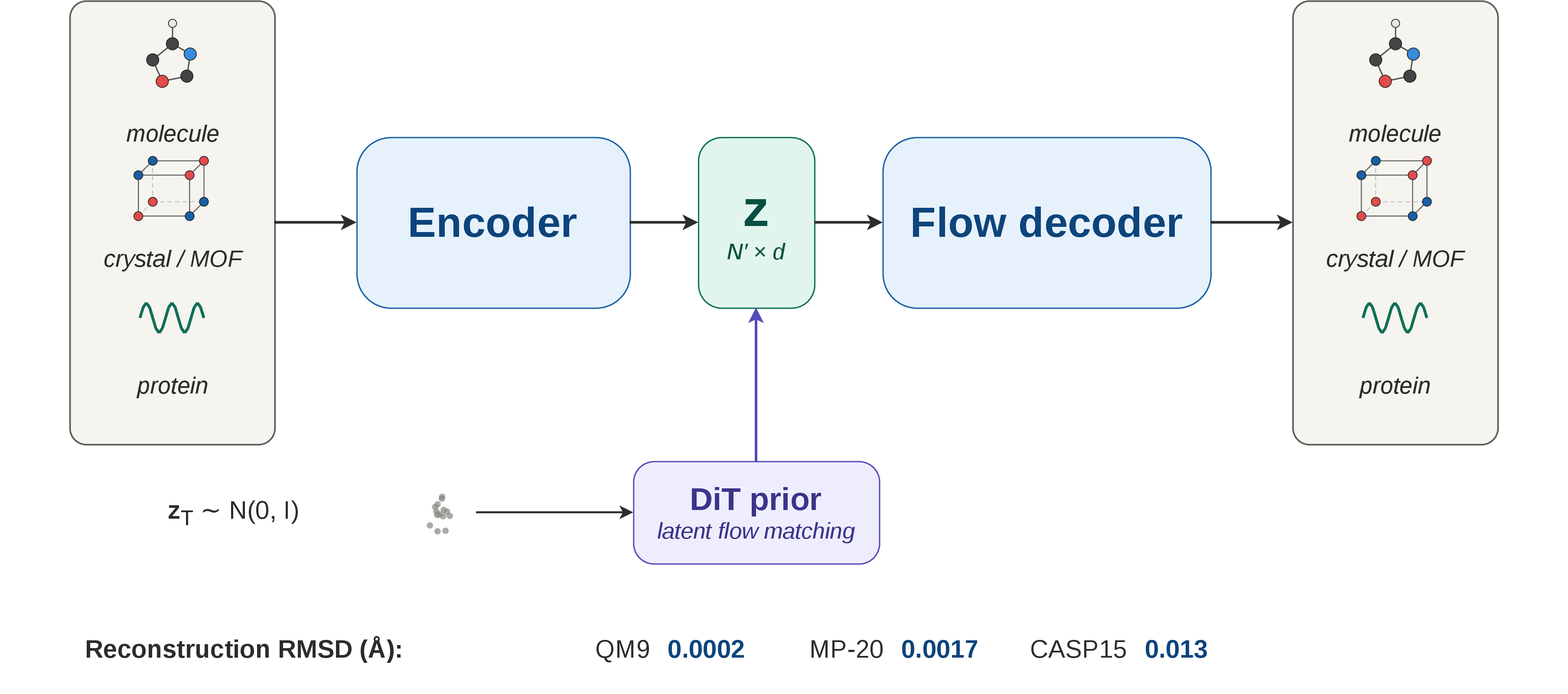
SinAE is trained for both reconstruction and generation. Given \(\mathcal{G}\), the autoencoder produces a latent code \(\mathbf{z}\) from which \(\mathcal{G}\) can be recovered with near-exact fidelity; a learned prior \(p(\mathbf{z})\) then enables de novo sampling of novel structures. These capabilities are provided by two components
trained in sequence:
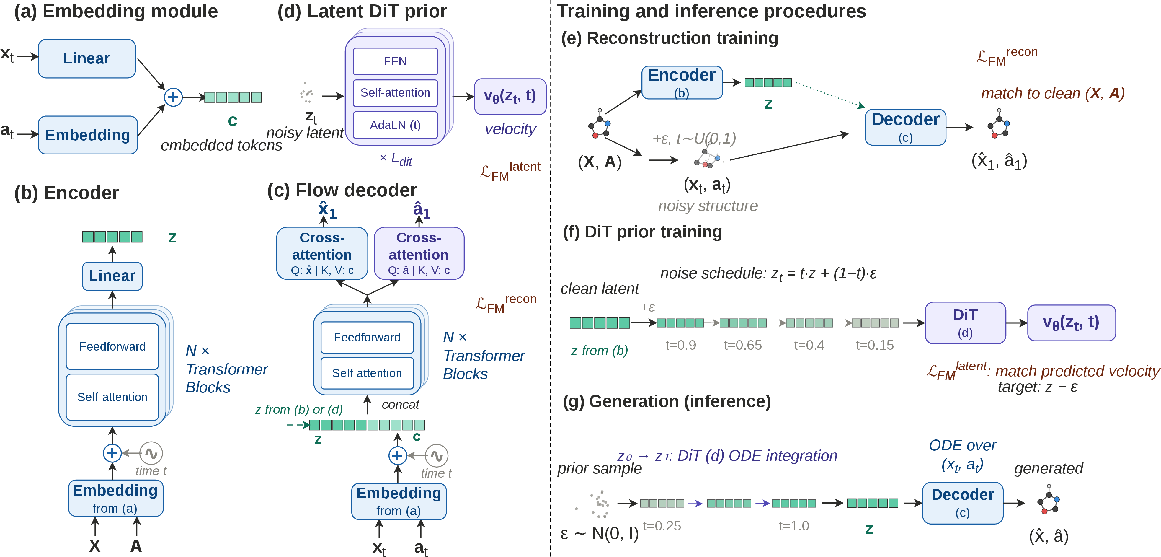
Flow-matching autoencoder. A Transformer encoder maps \(\mathcal{G}\) to a compact latent \(\mathbf{z}\), while a non-equivariant Transformer decoder reconstructs \(\mathcal{G}\) from \(\mathbf{z}\) via conditional flow matching. The decoder, not the encoder, is responsible for reconstruction fidelity, allowing the encoder to remain simple and domain-general.
Latent flow matching prior. A vanilla Diffusion Transformer (DiT) learns the distribution \(p(\mathbf{z})\) over encoder outputs. At generation time, a new latent is sampled from this prior and passed through the frozen decoder to produce a 3D structure.
The architecture and procedures are summarized in Figure 2.
3.2 Input Featurization↩︎
3.2.0.1 Coordinate handling.
We avoid hand-crafted geometric preprocessing. For aperiodic systems (molecules, proteins), the model consumes raw Cartesian coordinates \(\mathbf{x}_i \in \mathbb{R}^3\) after centering at the centroid, without PCA alignment, canonical-frame construction, or invariant descriptors (pairwise distances, sorted \(k\)-NN, bond angles). For periodic systems (crystals), we append the three lattice vectors \(\mathbf{L} = [\mathbf{l}_1, \mathbf{l}_2, \mathbf{l}_3]\) as three virtual-atom tokens at the end of the sequence, so the model processes the full \(3\times 3\) lattice matrix in the same way as atomic coordinates.
3.2.0.2 Equivariance via random augmentation.
To ensure the non-equivariant Transformer does not learn orientation-dependent features, we apply a random SO(3) rotation (and, for aperiodic systems, a random translation) to every training structure on the fly. Empirically this suffices to reach the reconstruction RMSD reported in Section 4.2 without any equivariant layer or invariant featurization.
3.2.0.3 Token construction.
Each atom \(i\) is represented by the sum of a learned element embedding (looked up from a table of size \(K\)) and a linear projection of its coordinate vector \(\mathbf{x}_i \in \mathbb{R}^3\), both projected to the Transformer model dimension \(d_{\mathrm{model}}\). The three lattice-vector tokens use a dedicated learned type embedding in place of the element lookup. For proteins, each residue is represented as a single token at its C\(\alpha\) position, with the residue type as the categorical label in place of the element type.
3.3 Architecture↩︎
3.3.0.1 Encoder.
The encoder \(\phi\) maps a sequence of \(N'\) input tokens to a sequence of latent tokens \(\mathbf{z}\in\mathbb{R}^{N'\times d}\), where \(N'=N\) for aperiodic systems and \(N'=N{+}3\) for periodic systems (the three trailing tokens encode the lattice vectors). A per-token (rather than pooled) latent preserves per-atom granularity: local geometric information scales with \(N\), so a fixed-size global bottleneck would force lossy compression for larger systems. We use a standard pre-norm Transformer with \(L_{\text{enc}}\) layers and multi-head self-attention; after the final layer, two parallel linear heads produce a Gaussian posterior \(\mathbf{z}_i = \boldsymbol{\mu}_i + \boldsymbol{\sigma}_i \odot \boldsymbol{\varepsilon}_i\), \(\boldsymbol{\varepsilon}_i\sim\mathcal{N}(\mathbf{0},\mathbf{I})\). We use a small latent channel \(d\) (see Appendix 12), keeping the total latent size compact while preserving enough information for near-exact decoding.
3.3.0.2 Flow-matching decoder.
The decoder \(\psi\) is a non-equivariant Transformer that reconstructs \((\mathbf{X}, \mathbf{A})\) from \(\mathbf{z}\) conditioned on partially noised inputs at time \(t\in[0,1]\). We follow DiTo’s [20] single-objective design but replace its score-matching formulation with a continuous conditional flow-matching objective for coordinates and a discrete flow-matching objective for atom types. The decoder receives noisy \((\mathbf{X}_t, \mathbf{A}_t)\) projected through separate linears, summed with a sinusoidal time embedding and a learnable positional embedding: \[\mathbf{h}_i^{(0)} = W_x\,\mathbf{x}_{t,i} + W_A\,\mathbf{a}_{t,i} + \mathbf{e}^{\text{time}}(t) + \mathbf{e}^{\text{pos}}_i, \label{eq:dec95input}\tag{1}\] where \(W_x\in\mathbb{R}^{d\times 3}\), \(W_A\in\mathbb{R}^{d\times K}\). The joint sequence \([\mathbf{h}^{(0)};\, \mathbf{z}]\) (concatenated along the sequence dimension, yielding \(2N'\) tokens) is processed by \(L_{\text{dec}}\) pre-norm Transformer blocks [28]. Following the two-stream output design of Tabasco [29], two parallel cross-attention output heads, one for coordinates and one for atom types, use the final hidden states as queries and the embedded noisy-input tokens \(\{\mathbf{c}_i\}\) as keys/values to produce \(\hat{\mathbf{X}}_1^\theta\) and \(\hat{\mathbf{A}}_1^\theta\) (Figure 2 (c)). No domain-specific attention, equivariant layer, or self-conditioning [30] is used in the backbone; random SO(3) augmentation at training time provides rotation robustness (Appendix 10).
3.4 Training Objective↩︎
The autoencoder is trained end-to-end by minimising a fixed-weight sum of three terms, \[\mathcal{L} = \mathcal{L}_{\text{coord}} + \lambda_{\text{atom}}\,\mathcal{L}_{\text{atom}} + \lambda_{\text{KL}}\,\mathcal{L}_{\text{KL}}, \label{eq:loss95total}\tag{2}\] where \(\mathcal{L}_{\text{coord}}\) is continuous conditional flow matching on coordinates [31], \(\mathcal{L}_{\text{atom}}\) is discrete flow matching on atom types [32], and \(\mathcal{L}_{\text{KL}}\) is a light KL regulariser pushing the encoder’s posterior towards \(\mathcal{N}(\mathbf{0},\mathbf{I})\). For periodic systems the three lattice-vector tokens are treated as virtual atoms, so their coordinates are reconstructed through the same \(\mathcal{L}_{\text{coord}}\) as ordinary atoms. Unlike DiTo [20], which uses a deterministic encoder, we use a stochastic encoder so that the aggregate posterior approximates the \(\mathcal{N}(\mathbf{0},\mathbf{I})\) prior of the DiT (Section 3.5). Exact loss definitions, interpolants, and weight values are in Appendix 11.
3.5 Latent Flow Matching for Generation↩︎
Because the KL term in Eq. 2 pushes the encoder’s posterior towards \(\mathcal{N}(\mathbf{0},\mathbf{I})\), the aggregate latent distribution is approximately Gaussian, and de novo generation reduces to learning \(p(\mathbf{z})\) and decoding. We train a vanilla DiT [21] \(v_\theta\) as a flow-matching velocity field [31] with the linear interpolant \(\mathbf{z}_t{=}(1{-}t)\mathbf{z}_0 + t\mathbf{z}_1\) and the standard FM objective \(\mathcal{L}_{\text{FM}}{=}\mathbb{E}\|v_\theta(\mathbf{z}_t,t){-}(\mathbf{z}_1{-}\mathbf{z}_0)\|^2\), without any equivariant layer or domain-specific module. Since \(\mathbf{z}\) is variable-length (\(N'{=}N\) or \(N{+}3\)), we pad and mask within each mini-batch during training. At generation time we sample the sequence length from the training-set size distribution before running the DiT ODE. Since the joint molecule–crystal model covers two domains, we condition the DiT prior on a domain label so that the user can specify which domain to generate at sampling time. During training, each sample carries its ground-truth domain label; at inference, we apply classifier-free guidance [33] on this label to steer generation toward the target domain.
A new structure is generated by sampling \(\mathbf{z}_0{\sim}\mathcal{N}(\mathbf{0},\mathbf{I})\), integrating \(v_\theta\) with fixed-step Euler to obtain \(\mathbf{z}_1\), and decoding from pure noise \((\mathbf{X}_0,\mathbf{A}_0)\) conditioned on \(\mathbf{z}_1\). Because the decoder is near-lossless, generated structures match the geometric precision of reconstructed training structures without post-hoc relaxation.
4 Experiments↩︎
We evaluate SinAE on three primary structural domains (small molecules, crystals, proteins) and one secondary domain (metal–organic frameworks; Appendix 20), focusing on two capabilities: (1)
reconstruction fidelity of the flow-matching autoencoder, and (2) de novo generation quality of the latent DiT prior.
4.1 Datasets, Training, and Evaluation Protocol↩︎
Datasets. We train and evaluate on standard benchmarks: QM9 [11] and GEOM-Drugs [34] for small molecules, MP-20 [4] (from the Materials Project [35]) for crystals, and AFDB-FS (a filtered single-chain subset of the AlphaFold Protein Structure Database [9], [10]) for proteins, with CASP14/CASP15 held out for protein reconstruction evaluation. As an additional periodic benchmark we use QMOF [36] for MOF reconstruction and generation; the full QMOF results and a head-to-head MOF generation comparison with ADiT are reported in Appendix 20. All splits follow prior work [4], [13], [22], [24], [37], [38]; full specification in Appendix 9.
Training and evaluation. We train autoencoder–prior pairs with the same vanilla-Transformer architecture but domain-appropriate sizing, using Adam/AdamW with constant learning rate \(10^{-4}\) , on a single NVIDIA H200 for \({\sim}48\) GPU-hours. Full hyperparameters, loss weights, flow-matching schedule, and evaluation protocol are in Appendix 12.
4.2 Reconstruction Fidelity↩︎
Figure 3 and Tables ¿tbl:tab:recon95nonprot?–2 report reconstruction across all four domains. On every dataset, SinAE reaches sub-milli-Å RMSD for
molecules and crystals and \(0.010\)–\(0.014\) Å CA-RMSD on proteins (chains truncated to the training-time maximum of \(256\) residues; longer chains
require retraining at a higher length budget, which we leave to future work), one to three orders of magnitude tighter than prior latent autoencoders.
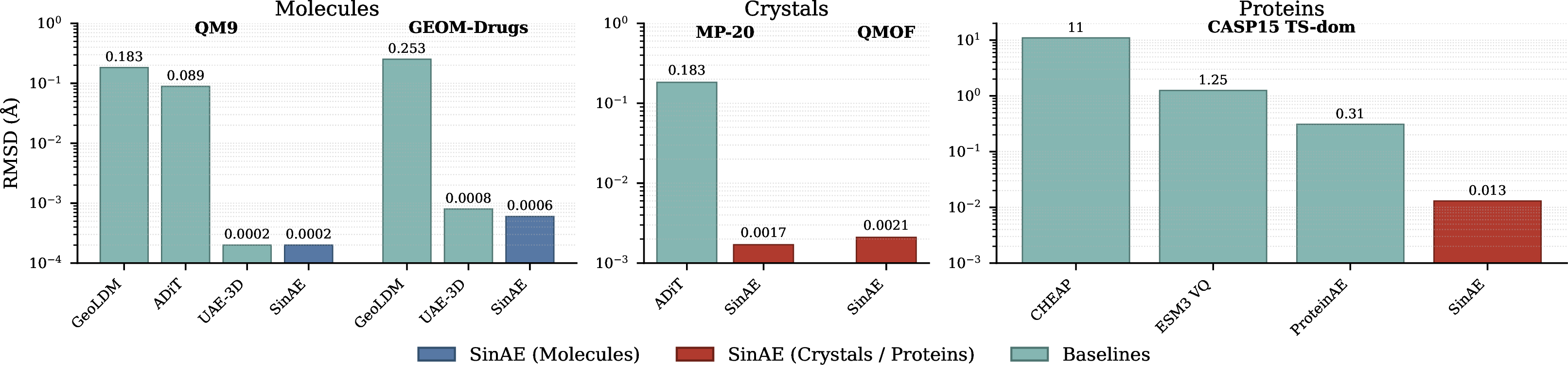
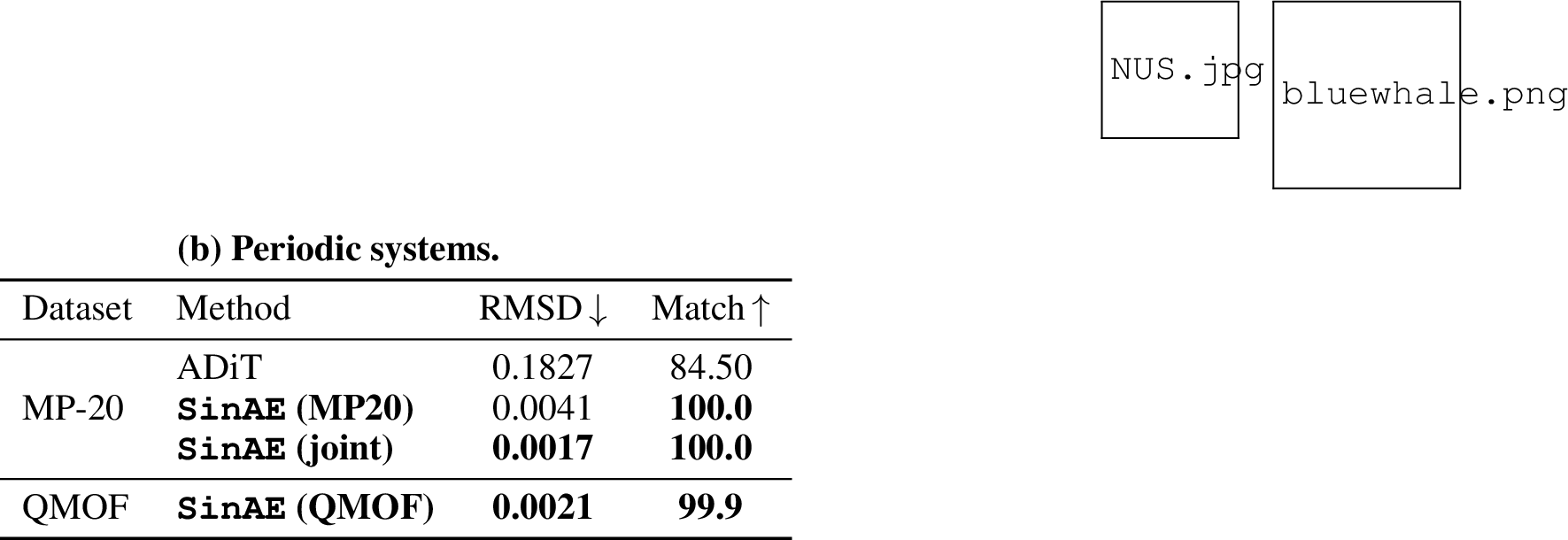
Isolating the flow-matching decoder. On molecules, SinAE matches or outperforms prior latent autoencoders [12], [18] while reaching \(100\%\) structure match rate on both QM9 and GEOM-Drugs (Table ¿tbl:tab:recon95nonprot?).
ADiT [13] also uses a vanilla Transformer over Cartesian coordinates with a shared latent across molecules and crystals, but
relies on a single-pass VAE decoder; it reaches \(94.6\%\) match rate on QM9 and \(84.5\%\) on MP-20, compared to \(100\%\) for SinAE on both.
This gap isolates the contribution of the iterative flow-matching decoder. Reconstruction RMSD saturates by roughly six decoder steps (Appendix 13).
Cross-domain transfer. Joint QM9 + MP-20 training improves both domains relative to single-domain training: QM9 RMSD drops from \(0.0007\) to \(\mathbf{0.0002}\) Å, and MP-20 RMSD from \(0.0041\) to \(\mathbf{0.0017}\) Å. Section 5.1 provides visual evidence through latent-space visualisation.
3pt

| CASP14 | CASP15 | ||||
|---|---|---|---|---|---|
| 2-4 (lr)5-6 Method | T | T-dom | oligo | TS-dom | oligo |
| CHEAP | 11.16 | 4.71 | 11.10 | 10.98 | 8.24 |
| ESM3 VQ-VAE | 1.28 | 0.66 | 3.11 | 1.25 | 2.47 |
| DPLM-2 | 1.94 | 1.47 | 3.81 | 4.58 | 3.83 |
| ProteinAE | 0.51 | 0.23 | 0.31 | 0.31 | 0.43 |
| 0.010 | 0.011 | 0.013 | 0.013 | 0.014 | |
3pt
4.3 Generative Performance: Molecules↩︎
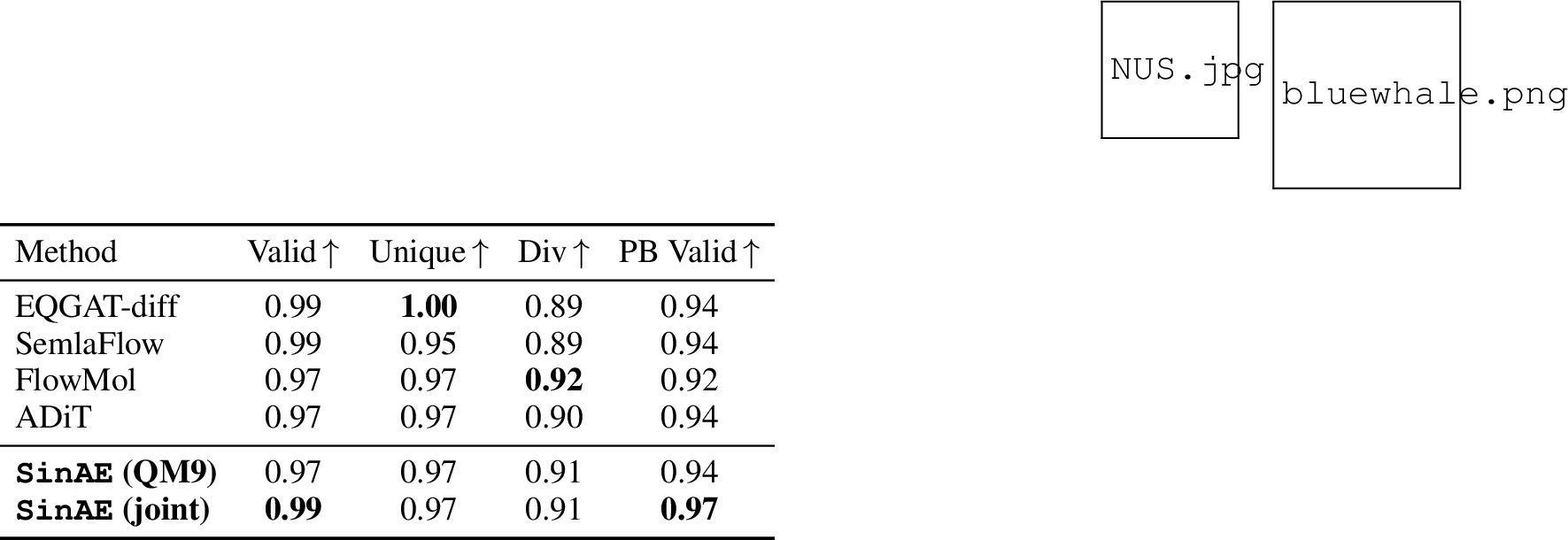
With near-lossless reconstruction established, we next ask whether the resulting latent space is smooth enough for a standard DiT prior to produce chemically valid structures. Tables ¿tbl:tab:gen95mol95qm9? and [tbl:tab:gen95mol95geom] report molecular generation on QM9 and GEOM-Drugs. The metric we emphasise is PB Valid (PoseBusters validity), which
simultaneously checks bond lengths, bond angles, and intra-molecular clashes and is therefore the strictest test of geometric quality. On QM9, the joint SinAE model reaches PB Valid 0.97, above all compared baselines including
equivariant methods (EQGAT-diff [23] and SemlaFlow [24] at \(0.94\), and FlowMol [25] at \(0.92\)). On GEOM-Drugs the margin widens: SinAE achieves PB Valid 0.93 against ADiT [13]’s \(0.86\) and SemlaFlow’s \(0.88\). That a non-equivariant architecture matches or exceeds equivariant generators on geometric quality reflects the
two-stage design: the autoencoder’s iterative decoder has already learned to produce geometrically precise structures during reconstruction training, and the DiT prior inherits this precision through the latent interface without needing to rediscover
bond-length or angle constraints. Validity, uniqueness, diversity, and novelty are competitive across both benchmarks (Tables ¿tbl:tab:gen95mol95qm9?–[tbl:tab:gen95mol95geom]); the per-PoseBusters-check breakdown is reported in Appendix 19.


4.4 Generative Performance: Materials↩︎
Crystal generation requires producing not only valid arrangements but thermodynamically metastable structures that survive DFT relaxation. Table 3 reports MP-20 results using S.U.N.(Stable, Unique, Novel) and
M.S.U.N.(S.U.N.with the stability threshold relaxed to \(E_{\mathrm{hull}}{<}0.1\) eV/atom). The joint SinAE model achieves S.U.N. / M.S.U.N., the highest among all compared
methods, surpassing FlowMM [26] (\(2.8\) / \(22.5\)) and
FlowLLM [27] (\(4.7\) / \(26.3\)) despite using a generic
Transformer with no lattice invariance or symmetry priors. The joint model improves over MP-20-only on every metric (S.U.N. \(4.6 \to 5.4\), M.S.U.N.\(24.31 \to 30.2\)), consistent with the
reconstruction gains in Section 4.2. Structure / composition validity (\(99.29\) / \(90.49\)) sits just below jointly-trained ADiT [13] (\(99.74\) / \(92.14\)), with SinAE’s advantage
concentrated in the stability-filtered metrics that probe thermodynamic plausibility rather than structural or compositional validity alone.
| Model | Struct \(\uparrow\) | Comp \(\uparrow\) | Stable \(\uparrow\) | M.S.U.N. \(\uparrow\) | S.U.N. \(\uparrow\) |
|---|---|---|---|---|---|
| CDVAE\(^\dagger\) | 100.00 | 86.70 | 1.6 | – | – |
| DiffCSP\(^\dagger\) | 100.00 | 83.25 | 5.0 | – | 3.3 |
| UniMat\(^\dagger\) | 97.2 | 89.4 | – | – | – |
| FlowMM | 96.85 | 83.19 | 4.6 | 22.5 | 2.8 |
| FlowLLM | 99.94 | 90.84 | 13.9 | 26.3 | 4.7 |
| Jointly-trained ADiT | 99.74 | 92.14 | 15.4 | 28.2 | 5.3 |
| (MP20-only) | 98.29 | 88.89 | 14.1 | 24.3 | 4.6 |
| (joint) | 99.29 | 90.49 | 15.8 | 30.2 | 5.4 |
| \(^\dagger\) CDVAE [4], DiffCSP [5], UniMat [39]. | |||||
5pt
4.5 Generative Performance: Proteins↩︎
The protein autoencoder uses the same architecture as the molecule–crystal model, so strong performance here confirms that the SinAE architecture generalises across domains rather than being tuned for small-molecule or crystal
chemistry.
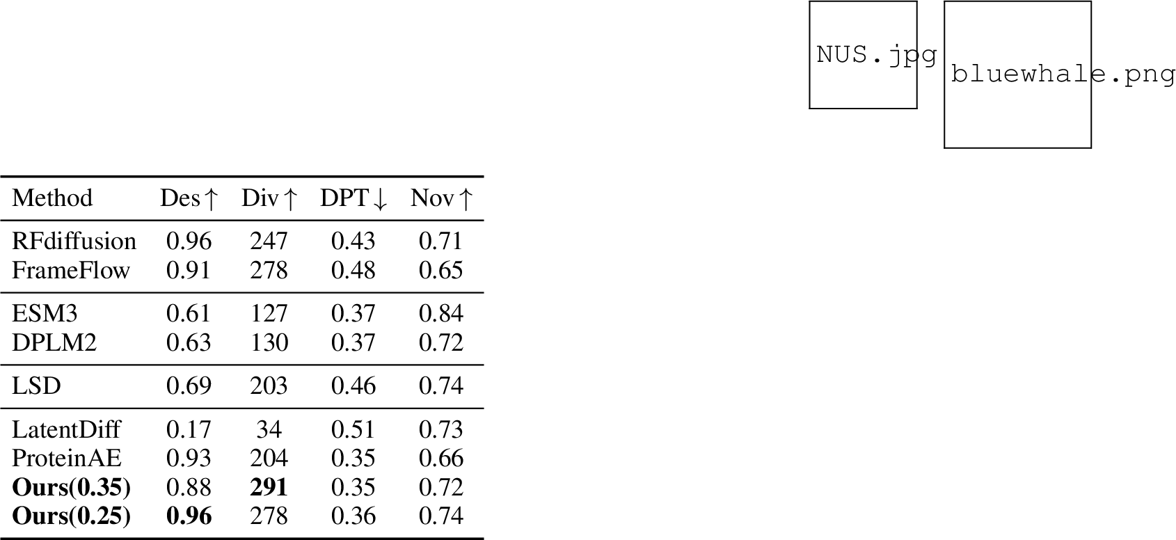
Unconditional generation. Table ¿tbl:tab:gen95prot? reports designability, diversity, DPT, and novelty. Prior latent-space protein generators face a trade-off between designability and diversity: ProteinAE achieves
\(0.93\) designability but with \(204\) diversity clusters, while LatentDiff produces diverse but largely non-designable backbones (\(0.17\) designability).
At guidance temperature \(0.25\), SinAE reaches 0.96 designability and \(278\) diversity, exceeding ProteinAE on both metrics simultaneously; at temperature
\(0.35\) it attains the highest diversity (291) among all compared methods while maintaining \(0.88\) designability. Two factors contribute: the near-lossless decoder
ensures that diversity in latent space translates into structural diversity without geometric degradation, and jointly modelling residue types alongside coordinates may steer generation toward more physically plausible backbone geometries compared to
coordinate-only approaches.
Co-design generation. Table [tbl:tab:performance] evaluates sequence–structure co-design at fixed lengths \(100\) and \(200\). At length \(100\), SinAE reaches scRMSD \(3.93\) Å and scTM \(0.83\), comparable to MultiFlow [32] (\(0.86\) / \(4.73\) Å) and ProteinGenerator [40] (\(0.91\) /
\(3.75\) Å). At length \(200\), scRMSD is \(4.44\) Å, below both MultiFlow (\(4.98\) Å) and ProteinGenerator (\(6.24\) Å). scTM (\(0.83\) / \(0.78\)) is below APM [41] (\(0.96\) / \(0.89\)), a method with protein-specific architecture.

5 Analysis↩︎
5.1 Latent Space Structure↩︎
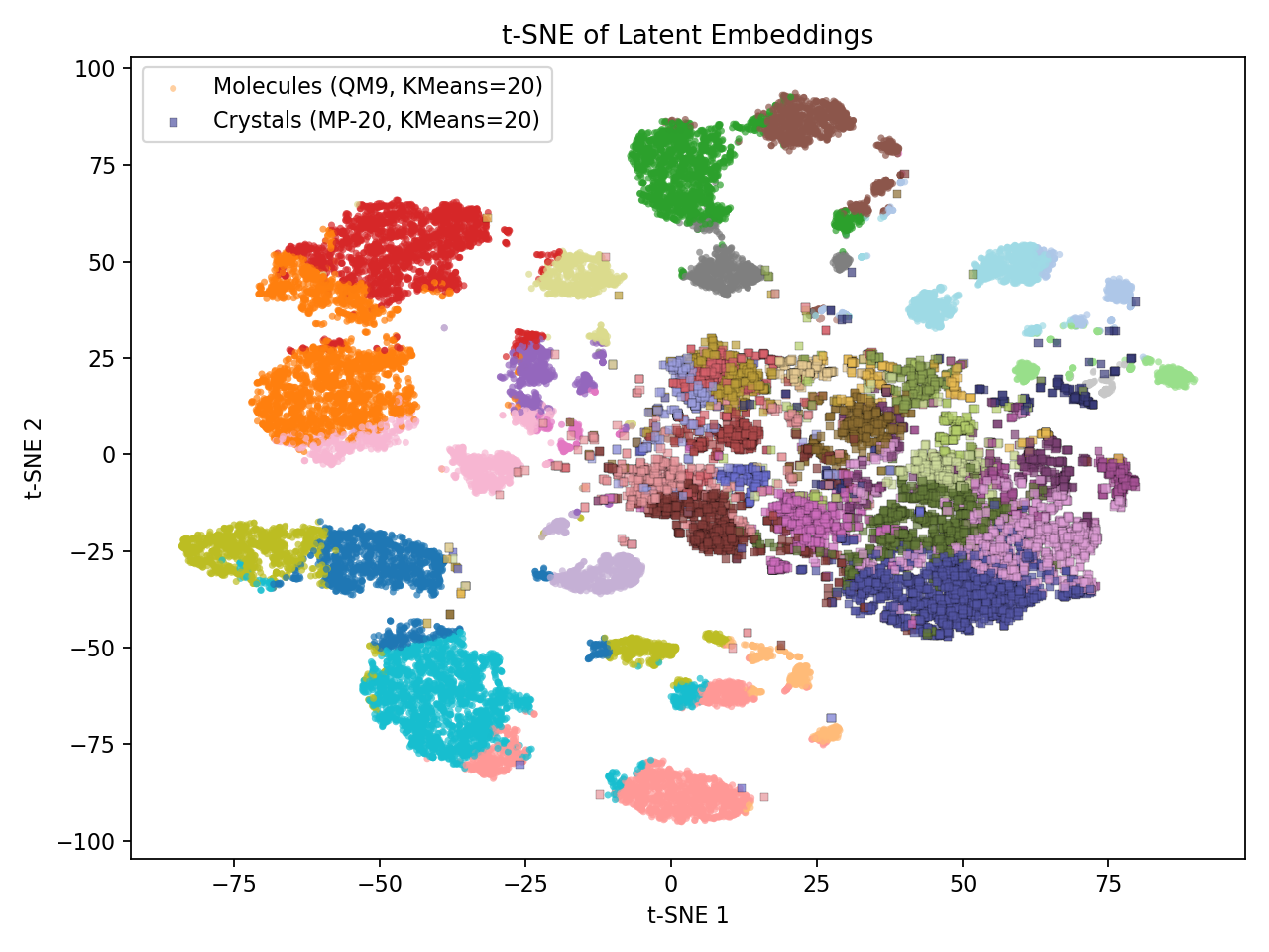
Sections 4.2 and 4.4 showed that joint QM9+MP-20 training improves both domains in reconstruction and generation. A t-SNE projection of the joint model’s encoder outputs (Appendix 14) shows that molecules and crystals occupy separated, internally coherent regions without any explicit domain label. Within each domain, KMeans clusters align with chemically meaningful groupings: functional-group composition for molecules, coordination environment for crystals. The two domains share a common low-density boundary region, suggesting that the encoder learns geometric regularities (bond-length distributions, coordination patterns) transferable across domains. This shared structure is consistent with the reconstruction improvement (\(0.0007 \to 0.0002\) Å on QM9, \(0.0041 \to 0.0017\) Å on MP-20) and the generation gain (M.S.U.N.\(24.31 \to 30.2\)) when the two populations are pooled through a single latent. Straight-line interpolations between encoded structures decode into valid intermediates across all three domains (Appendix 15).
5.2 Decoder Trajectory Analysis↩︎
Figure 5 examines the decoder’s behaviour during generation (decoding from DiT-sampled latents, not from encoded ground-truth structures). We track two quantities along the decoder ODE trajectory \(t \in [0,1]\): physical energy (top row) and Kabsch-aligned RMSD to the final state at \(t{=}1\) (bottom row). For molecules, force-field energy drops by more than ten orders of magnitude; for crystals, CHGNet energy descends from \({\sim}6\) eV/atom into the sub-\(1\) eV/atom metastable window. Crucially, the two quantities follow different schedules: RMSD plateaus near zero by \(t \approx 0.8\) while energy continues to descend through the final \(20\%\) of the trajectory. Early ODE steps thus handle geometric placement, while late steps perform fine local refinement (bond-angle planarity, dihedral relaxation, sterics) that contributes little to RMSD but substantially to physical energy. The decoder learns denoising directions aligned with the local energy gradient even though energy is never supervised, and this holds for prior-sampled latents that the encoder has never produced.
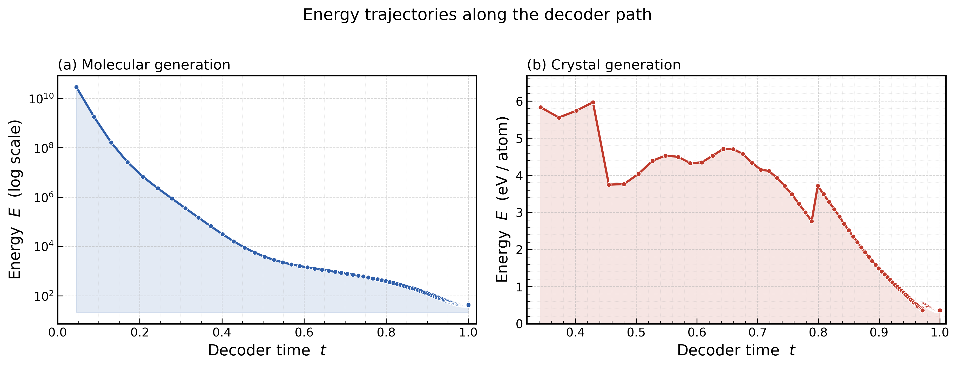
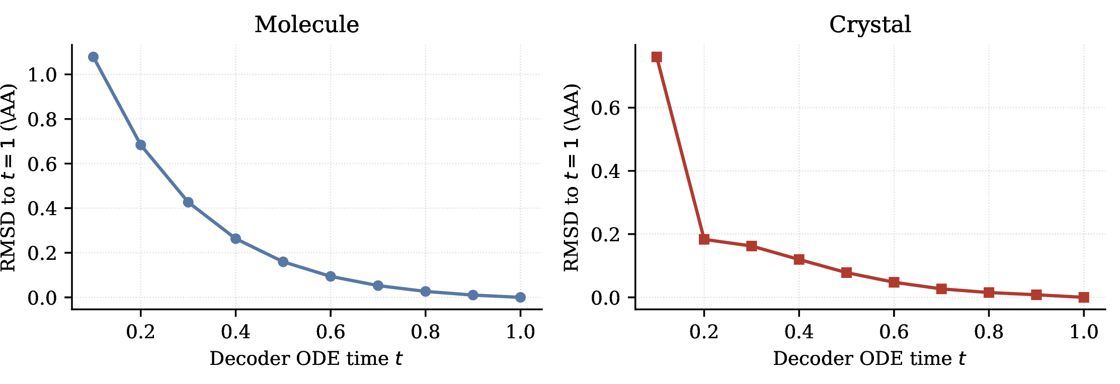
Figure 5: Decoder ODE trajectory during generation (DiT-sampled latents, not encoded ground truth). (a) Physical energy along the trajectory (molecule force-field, log scale; crystal CHGNet, eV/atom). (b) Kabsch-aligned RMSD to the final state at \(t{=}1\). RMSD plateaus by \(t \approx 0.8\) while energy continues to descend: early steps handle geometric placement, late steps perform fine local refinement. Energy was never used as a training signal..
6 Conclusion↩︎
We presented SinAE, a vanilla-Transformer flow-matching autoencoder for molecules, crystals, and proteins. By shifting reconstruction fidelity into an iterative flow-matching decoder trained with a unified objective, SinAE
reaches sub-milli-Å Kabsch-aligned RMSD on molecules and crystals and \(\sim 0.02\) Å backbone CA-RMSD on proteins, while supporting strong latent generation across all three domains. Joint training on QM9 + MP-20 improves
both domains in reconstruction and generation, providing direct evidence that cross-domain training through a shared atomic latent benefits both chemical populations. Limitations. Protein evaluation is at the backbone level; all-atom
protein modelling, property- / composition- / length-conditioned generation, and single-checkpoint training across all three domains are natural directions for future work.
Appendix
7 Broader Impacts↩︎
SinAE is an architectural contribution towards 3D structural representation learning; its immediate downstream use cases are molecular, materials, and protein design in academic and industrial R&D. Positive societal impacts include
accelerating the discovery of catalysts for carbon capture and clean energy, stable metal–organic frameworks for gas storage, and therapeutic lead compounds. We note, however, that the same generative capabilities could in principle be misused to
accelerate the design of toxic small molecules, narcotics, or proteins with harmful biological activity. The models released alongside this work are trained exclusively on publicly available non-hazardous datasets (QM9, GEOM-Drugs, MP-20, QMOF, AFDB-FS),
none of which is enriched for hazardous compounds, and we do not anticipate SinAE conferring a meaningful advantage over existing, widely available generative tools for adversarial design. We encourage downstream users to combine generative
models of this class with structure-aware toxicity and bioactivity filters before experimental validation, and we are not releasing any fine-tuned weights targeted at restricted chemical or biological endpoints.
8 Evaluation Metrics↩︎
This appendix defines every metric reported in the main text and specifies the tool, formula, or threshold used for each.
8.1 Reconstruction Metrics↩︎
8.1.0.1 Coordinate RMSD (Å, \(\downarrow\)).
For a structure with \(N\) atoms, ground-truth coordinates \(\mathbf{X}\in\mathbb{R}^{N\times 3}\), and reconstructed coordinates \(\hat{\mathbf{X}}\in\mathbb{R}^{N\times 3}\), we first align \(\hat{\mathbf{X}}\) to \(\mathbf{X}\) using the Kabsch algorithm (optimal rotation \(R^{*}\), translation \(t^{*}\) via SVD), then report \[\mathrm{RMSD}(\mathbf{X}, \hat{\mathbf{X}}) \;=\; \sqrt{\tfrac{1}{N}\sum_{i=1}^{N}\bigl\|\mathbf{x}_i - (R^{*}\hat{\mathbf{x}}_i + t^{*})\bigr\|_2^{2}}.\] For proteins we apply this to the \(C_\alpha\) trace (CA-RMSD). For periodic systems (crystals, MOFs), coordinates are first unwrapped into a single fractional cell and Kabsch alignment is applied in the Cartesian space.
8.1.0.2 Structure Match Rate — Reconstruction (%, \(\uparrow\)).
For molecule reconstruction on QM9, the structure match rate uses pymatgen.analysis.molecule_matcher. MoleculeMatcher.get_rmsd with InChI-based atom mapping at tolerance \(0.01\) Å. A reconstructed
molecule is counted as a match iff this routine returns a finite RMSD, i.e.the predicted 3D conformation is chemically isomorphic to the reference under the OpenBabel bond-perception convention (identical atom counts, atomic numbers, and inferred bond
multiset).
For MP-20 crystal reconstruction, we compute the structure match rate using StructureMatcher from pymatgen, with thresholds \(l_{\mathrm{tol}}=0.3\), \(s_{\mathrm{tol}}=0.5\), and \(\mathrm{angle}_{\mathrm{tol}}=10^\circ\). A 100% match rate means that every reconstructed crystal is matched to its reference under these tolerances.
8.1.0.3 Valid (%, \(\uparrow\)).
Fraction of generated molecules accepted by RDKit’s sanitization pipeline (valid valences, no kekulisation failure, parseable SMILES).
8.1.0.4 Unique (%, \(\uparrow\)).
Fraction of valid molecules whose canonical SMILES is distinct from the other molecules in the sampled batch. Computed on the same \(N\) samples used for Valid.
8.1.0.5 Novelty (%, \(\uparrow\)).
Fraction of valid molecules whose canonical SMILES does not appear in the training set.
8.1.0.6 Diversity (\(\uparrow\)).
Mean pairwise Tanimoto dissimilarity of Morgan fingerprints (radius 2, 2048 bits) across the valid generated molecules: \[\mathrm{Diversity} = 1 - \tfrac{2}{N(N-1)}\sum_{i<j} \mathrm{Tanimoto}(\mathbf{f}_i, \mathbf{f}_j).\]
8.1.0.7 PB Valid (%, \(\uparrow\)).
PoseBusters-Validity: a molecule is PB-valid only if it simultaneously passes all PoseBusters sanity checks: chemistry, intra-molecular clashes, bond lengths and angles within empirical distributions. PB Valid is the most physically restrictive metric in Tables ¿tbl:tab:gen95mol95qm9?–[tbl:tab:gen95mol95geom] and is the metric we emphasise for geometric quality.
8.2 Crystal Generation Metrics↩︎
8.2.0.1 Structure / Composition / Overall Validity (%, \(\uparrow\)).
Structure validity counts generated crystals that pass pymatgen’s structure-level sanity (no atomic overlap, finite lattice). Composition validity counts crystals whose composition is charge-balanced with standard oxidation states. Overall validity is the product (i.e.passes both). We follow the protocol of CDVAE.
8.2.0.2 Stable and Metastable Rate (%, \(\uparrow\)).
We follow the two-stage relaxation protocol of ADiT [13]: each generated crystal is first pre-relaxed with the CHGNet universal machine-learning potential [43], and the pre-relaxed geometry is then DFT-relaxed. Stability is evaluated against the Matbench-Discovery convex hull using the final DFT energy-above-hull \(E_{\mathrm{hull}}\): \[\text{stable}: E_{\mathrm{hull}} < 0.0\text{ eV/atom and } \#\text{unique elements} \ge 2,\] \[\text{metastable}: E_{\mathrm{hull}} < 0.1\text{ eV/atom and } \#\text{unique elements} \ge 2.\] The \(\ge 2\) unique-element constraint matches ADiT and excludes trivial elemental crystals from stability counting.
8.2.0.3 S.U.N.and M.S.U.N.(%, \(\uparrow\)).
S.U.N. (Stable, Unique, Novel) is the fraction of sampled crystals that are simultaneously (i) stable under the above definition, (ii) structurally unique within the sample batch, and (iii) novel with respect to the MP-20 training set.
Uniqueness and novelty both use pymatgen.StructureMatcher with the thresholds listed in 8.1 for an all-to-all equivalence check. M.S.U.N. replaces “stable” with “metastable” in condition (i).
Following FlowMM, FlowLLM, and ADiT, these are the hard metrics for crystal generation and the ones we emphasise when claiming state of the art.
8.3 Protein Generation Metrics↩︎
For each generated backbone we run ProteinMPNN inverse folding (\(8\) sequences per backbone) and fold the resulting sequences with ESMFold; all self-consistency metrics below are computed over this design-fold loop, following the protocol of ProteinBench [42].
8.3.0.1 scRMSD (Å, \(\downarrow\)) and scTM (\(\uparrow\)).
Self-consistency RMSD is the Kabsch-aligned CA-RMSD between the generated backbone and the best ESMFold re-fold among the \(8\) designed sequences; scTM is the corresponding best TM-score. These are the two primary quality metrics in Table [tbl:tab:performance].
8.3.0.2 Designability (“Des”, \(\uparrow\)).
Fraction of generated backbones with \(\mathrm{scRMSD} \le 2.0\) Å, i.e.structures for which at least one designed sequence re-folds into essentially the same backbone. This is the standard “designable” criterion [6], [7].
8.3.0.3 Diversity (“Div”, \(\uparrow\)).
Number of unique structural clusters obtained by hierarchical clustering of the designable backbones using pairwise TM-score with a \(0.5\) cutoff (single linkage). A higher number indicates that more distinct folds have been reached.
8.3.0.4 DPT — Designable Pairwise TM-score (\(\downarrow\)).
Mean pairwise TM-score computed only over the subset of generated backbones that passed the designability filter (\(\mathrm{scRMSD} \le 2.0\) Å). Restricting the computation to designable samples removes low-quality, degenerate structures that would otherwise inflate pairwise dissimilarity; a lower DPT indicates that the useful outputs of the model explore a structurally wider region. DPT is complementary to Div (which counts cluster number) in that it measures the geometric spread of the designable samples.
8.3.0.5 Novelty (“Nov”, \(\uparrow\)).
\(1 - \max_{p\in\mathrm{PDB}}\mathrm{TM}(\hat{x}, p)\), the deviation of each generated backbone from its closest match in the full PDB (measured by TM-score); averaged across designable samples. Higher means further from any known fold.
8.4 Latent-Space Analysis Metrics↩︎
8.4.0.1 Per-atom classical force-field energy (eV/atom, \(\downarrow\)).
For molecule trajectories in Figure 5 we report the per-structure energy computed with a classical force field (UFF/MMFF as implemented in RDKit) evaluated on the decoder’s intermediate structures \((\mathbf{x}_t, \mathbf{a}_t)\). For crystal trajectories we report the per-atom energy from the same CHGNet ML potential used for stability evaluation above. These are reported only to probe whether the decoder’s ODE path visits progressively lower-energy configurations; they are not used as training signal at any stage.
9 Full Dataset Specification↩︎
This appendix provides the per-domain dataset details abbreviated in Section 4.1.
9.0.0.1 Molecules.
QM9 [11] consists of 130,000 stable small organic molecules containing up to nine heavy atoms (C, N, O, F) along with hydrogens. We follow the splits of [22]. GEOM-Drugs [34] is a dataset of 1M high-quality conformers of drug-like molecules; we use the splits of [37] and, following [24], discard molecules with more than 72 heavy atoms from the training set (accounting for 1% of the data). At test time we sample molecule sizes from the (unchanged) test-set size distribution.
9.0.0.2 Materials.
MP-20 [4] contains 45,231 metastable crystal structures from the Materials Project [35], each with up to 20 atoms per unit cell and spanning 89 elements; we use the CDVAE splits [4]. QMOF [36] is a database of 14,000 MOF structures with quantum-chemical properties; we use the splits of [13].
9.0.0.3 Proteins.
AFDB-FS [9], [10] is a filtered single-chain subset of the AlphaFold Protein Structure Database, obtained via sequence-based MMseqs2 and structure-based Foldseek [38] clustering. It contains 588,318 structures with lengths in \([32, 256]\). For training we apply random global SO(3) rotations as data augmentation. For reconstruction evaluation we use the CASP14 and CASP15 benchmark sets.
10 Method Design Rationale↩︎
This appendix collects the design justifications abbreviated in the main-paper architecture section.
10.0.0.1 Why a per-token latent instead of a pooled global code.
Atomistic structures exhibit local geometric features (bond environments, coordination shells) whose information content scales with the number of atoms \(N\); a fixed-size global latent would force lossy compression as \(N\) grows. Our latent is \(\mathbf{z}\in\mathbb{R}^{N'\times d}\) with compact per-token dimension \(d\) (see Appendix 12), which keeps the total latent size an order of magnitude smaller than the raw structure while preserving enough information for near-exact decoding. Because the decoder handles fine-grained geometry, the encoder can remain lightweight while producing a latent that is smooth and suitable for downstream generative modelling.
10.0.0.2 Why a non-equivariant Transformer.
Equivariant layers encode physical symmetries as hard constraints, but at substantial architectural-complexity and scaling cost. We instead rely on random SO(3) rotation augmentation during training (Section 3.2) to induce rotation robustness, and demonstrate empirically that this, combined with the iterative flow-matching decoder, is sufficient to achieve near-lossless reconstruction on molecules and crystals and sub-\(0.03\) Å RMSD on proteins.
10.0.0.3 Why output heads instead of stream-specific mid-backbone cross-attention.
Following Tabasco [29], we localise the coordinate / atom-type specialisation in two parallel cross-attention output heads rather than interleaving stream-specific cross-attention inside the backbone. This keeps every Transformer block in the backbone fully shared across its constituent structural categories, and places all cross-attention compute at the output, where it directly conditions the two prediction heads on the embedded noisy inputs.
10.0.0.4 Why we do not use self-conditioning.
We found a single-pass output head with cross-attention from the noisy input to be sufficient; self-conditioning [30] does not provide measurable gains on our atomistic reconstruction benchmarks in preliminary tests and increases per-step cost.
11 Full Training Objective↩︎
This appendix gives the exact interpolants, loss formulae, and weight values abbreviated in Section 3.4. All three terms are summed in Eq. 2 .
11.0.0.1 Coordinate flow matching [31].
With the interpolant \(\mathbf{X}_t = t\,\mathbf{X}_1 + (1-t)\,\boldsymbol{\epsilon}\), \(\boldsymbol{\epsilon}\sim\mathcal{N}(\mathbf{0},\mathbf{I})\), \(t\sim\mathcal{U}(0,1)\), the coordinate head is trained with \(x_1\)-prediction: \[\mathcal{L}_{\text{coord}} = \mathbb{E}_{\boldsymbol{\epsilon},\,t} \!\left[\tfrac{1}{N}\bigl\|\hat{\mathbf{X}}_1^\theta(\mathbf{X}_t, \mathbf{A}_t, t, \mathbf{z}) - \mathbf{X}_1\bigr\|_2^2\right]. \label{eq:loss95coord}\tag{3}\]
11.0.0.2 Atom-type discrete flow matching [32].
Ground-truth atom types are corrupted by interpolating with a uniform categorical prior, \(\mathbf{A}_t \sim \mathrm{Cat}(t\,\delta(\mathbf{A}_1) + (1-t)\,\tfrac{1}{K}\mathbf{1})\), and the head is trained with endpoint cross-entropy: \[\mathcal{L}_{\text{atom}} = \mathbb{E}_{t} \!\left[-\tfrac{1}{N}\sum_{i=1}^{N} \mathbf{A}_{1,i}^\top \log \hat{\mathbf{A}}_{1,i}^\theta(\mathbf{X}_t, \mathbf{A}_t, t, \mathbf{z})\right]. \label{eq:loss95atom}\tag{4}\]
11.0.0.3 KL regularisation.
Unlike DiTo [20], we pair a stochastic encoder with the decoder and add a light KL term pushing \(q_\phi(\mathbf{z}|\mathcal{G})\) towards \(\mathcal{N}(\mathbf{0},\mathbf{I})\): \[\mathcal{L}_{\text{KL}} = D_{\mathrm{KL}}\bigl(q_\phi(\mathbf{z}|\mathcal{G}) \,\|\, \mathcal{N}(\mathbf{0},\mathbf{I})\bigr) = \tfrac{1}{2}\sum_{j}\bigl(\mu_j^2 + \sigma_j^2 - \log\sigma_j^2 - 1\bigr). \label{eq:loss95kl}\tag{5}\] Aligning the aggregate posterior with a Gaussian simplifies the prior-fitting problem for the latent flow-matching model (Section 3.5).
Weight values (\(\lambda_{\text{atom}}{=}0.1\), \(\lambda_{\text{KL}}{=}10^{-6}\)) are listed alongside the rest of the training configuration in Appendix 12; we find the model insensitive to these weights across an order of magnitude each.
12 Full Implementation Details↩︎
This appendix gives the complete architectural, training, and evaluation specification for the SinAE models summarised in Section 4.1.
12.1 Architecture↩︎
The autoencoder uses a pre-norm vanilla Transformer with hidden dimension \(d_{\text{model}}{=}64\) and \(8\) attention heads throughout. No equivariant layer, message-passing operator, graph attention, or pretrained discriminator is used anywhere in the architecture.
Joint molecule–crystal autoencoder. Encoder depth \(L_{\text{enc}}{=}4\), decoder depth \(L_{\text{dec}}{=}16\), per-token latent dimension \(d{=}8\) (so \(\mathbf{z}\in\mathbb{R}^{N'\times 8}\)).
Joint molecule–crystal latent DiT. \(L_{\text{dit}}{=}24\) layers, \(d_{\text{model}}{=}1024\), \(16\) attention heads.
Protein autoencoder. Encoder depth \(L_{\text{enc}}{=}4\), decoder depth \(L_{\text{dec}}{=}16\), per-token latent dimension \(d{=}16\).
Protein latent DiT prior. \(L_{\text{dit}}{=}15\) layers, \(d_{\text{model}}{=}768\), \(12\) attention heads.
12.2 Training↩︎
All stages use Adam (autoencoder) and AdamW (latent prior) with a constant learning rate of \(1{\times}10^{-4}\), weight decay \(0\), no warm-up, and no scheduler. The joint molecule–crystal autoencoder is trained with batch size \(2048\) (each batch drawn \(50\)/\(50\) from QM9 and MP-20); the protein autoencoder uses batch size \(256\).
The total reconstruction loss follows Eq. 2 with the fixed weights \[\lambda_{\text{coord}}{=}1.0,\quad \lambda_{\text{atom}}{=}0.1,\quad \lambda_{\text{KL}}{=}1{\times}10^{-6}.\] The flow-matching schedule uses a lower time cutoff \(t_{\min}{=}10^{-2}\); no additional \(\sigma_{\min}\) is imposed.
The joint molecule–crystal model was trained on a single NVIDIA H200 GPU for approximately \(48\) GPU-hours.
12.3 Evaluation Protocol↩︎
12.3.0.1 Reconstruction RMSD.
All reconstruction RMSDs are computed after Kabsch SVD alignment between the decoded and reference coordinates. Protein CA-RMSD uses the same Kabsch pipeline on the \(C_\alpha\) trace.
12.3.0.2 Crystal Structure-Match Rate.
Both crystal generation and crystal reconstruction structure-match rates use the same pymatgen.StructureMatcher pipeline with the standard thresholds \(\mathrm{ltol}{=}0.3\), \(\mathrm{stol}{=}0.5\), \(\mathrm{angle\_tol}{=}10^{\circ}\) [4]; we
additionally report Kabsch-aligned RMSD for reconstruction as a continuous fidelity metric.
12.3.0.3 Generation NFE.
At generation time we use NFE\({=}100\) Euler steps for both the DiT latent prior and the flow-matching decoder of the joint molecule–crystal model. Protein latent sampling uses a smaller latent step size \(\mathrm{dt}_{\text{latent}}{=}2.5{\times}10^{-3}\) (NFE\({=}400\)), because the longer protein latents empirically benefit from more steps. Classifier-free guidance (used only for domain-selection in the joint molecule–crystal model) doubles per-step compute but does not change NFE.
13 Fidelity–Efficiency Trade-off (Decoder NFE)↩︎
Because reconstruction is iterative, inference cost scales linearly with the number of function evaluations (NFE) in the decoder. Figure 6 plots reconstruction RMSD against NFE on QM9 and MP-20. On both datasets, RMSD drops
sharply between NFE\({=}1\) and NFE\({=}4\) and saturates by NFE\({\approx}6\): the QM9 decoder reaches its asymptotic RMSD of \(\sim 0.0003\) Å after only \(6\) steps, and MP-20 saturates at \(\sim 0.0016\) Å over the same range. Even at NFE\({=}2\),
SinAE already outperforms every VAE baseline in Table ¿tbl:tab:recon95nonprot?, confirming that the fidelity advantage is not from expensive sampling. In practice we use NFE\({=}10\) as a
comfortable operating point.
In wall-clock terms, at NFE\({=}10\) on a single NVIDIA H200 the decoder takes \(0.13\) s per batch of \(4\) QM9-scale molecules (\(\sim 36\) atoms total), i.e.\(\sim 32\) ms per molecule, or \(\sim 3.6\) ms per atom. Generating \(10\) k molecules takes \(\sim 5\) minutes including overhead.

14 t-SNE of the Joint Latent Space↩︎
Section 5.1 interprets the cross-domain transfer through a t-SNE projection of the joint molecule + crystal model’s encoder outputs. Figure 7 visualises this projection: QM9 molecules (circles) and MP-20 crystals (squares) occupy separated, internally coherent regions of the latent space without any explicit domain label. Colours indicate within-domain KMeans clusters; molecular clusters separate by functional-group composition while crystal clusters align with coordination environment. The two domains share a low-density boundary region, consistent with shared low-level geometric regularities (bond-length distributions, coordination patterns) being captured by a common encoder.
15 Latent-Space Interpolation Across Domains↩︎
Section 5.1 reports that straight-line interpolations between pairs of SinAE latents decode into chemically and geometrically valid intermediates across all three domains; we visualise representative
trajectories in Figure 8. Molecular interpolations preserve ring connectivity while smoothly varying functional groups; crystal interpolations transition between unit-cell geometries while keeping atoms well-coordinated;
protein interpolations evolve continuously from highly helical backbones toward more compact mixed-fold structures. This smoothness is consistent with the strong generative results in Section 4.
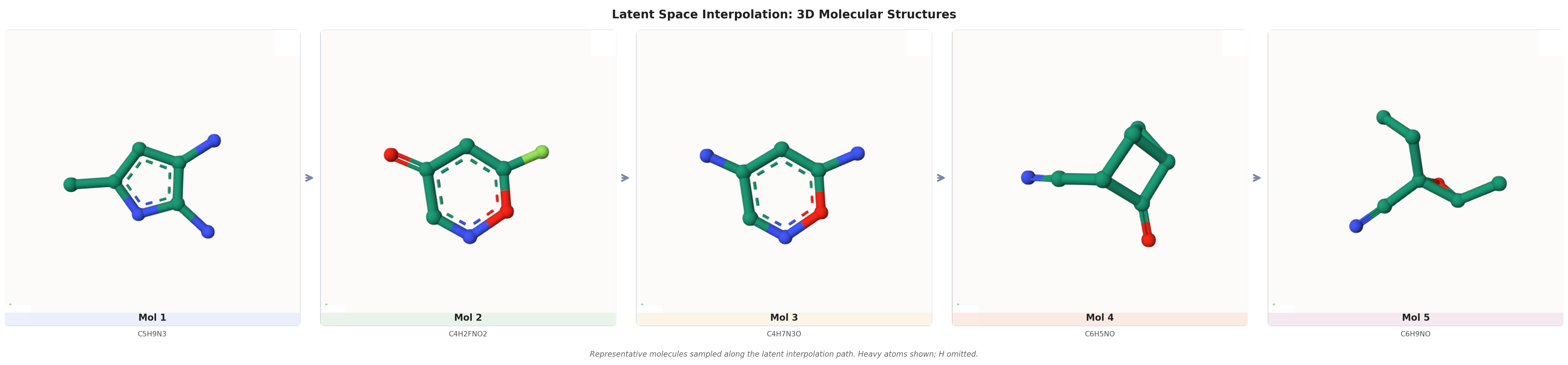
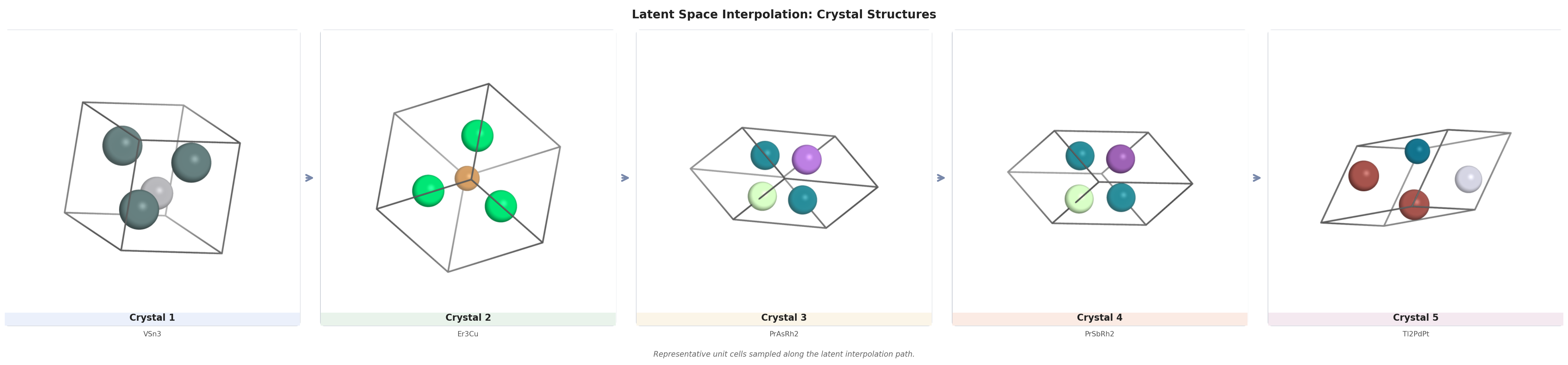
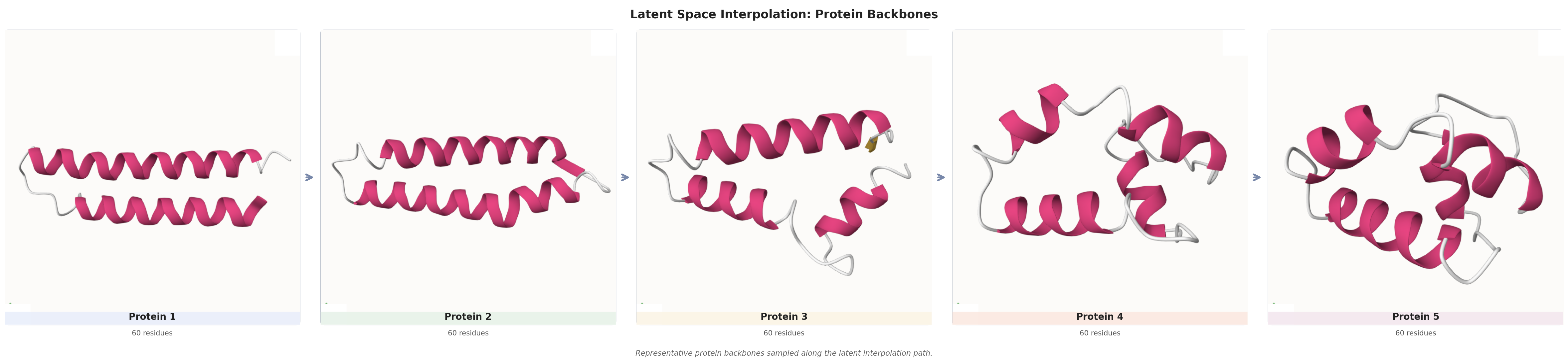
Figure 8: Latent-space interpolation across domains. Structures decoded along straight-line interpolations between pairs of SinAE latents: molecules (top), crystals (middle), proteins (bottom)..
16 Length Generalisation on Proteins↩︎
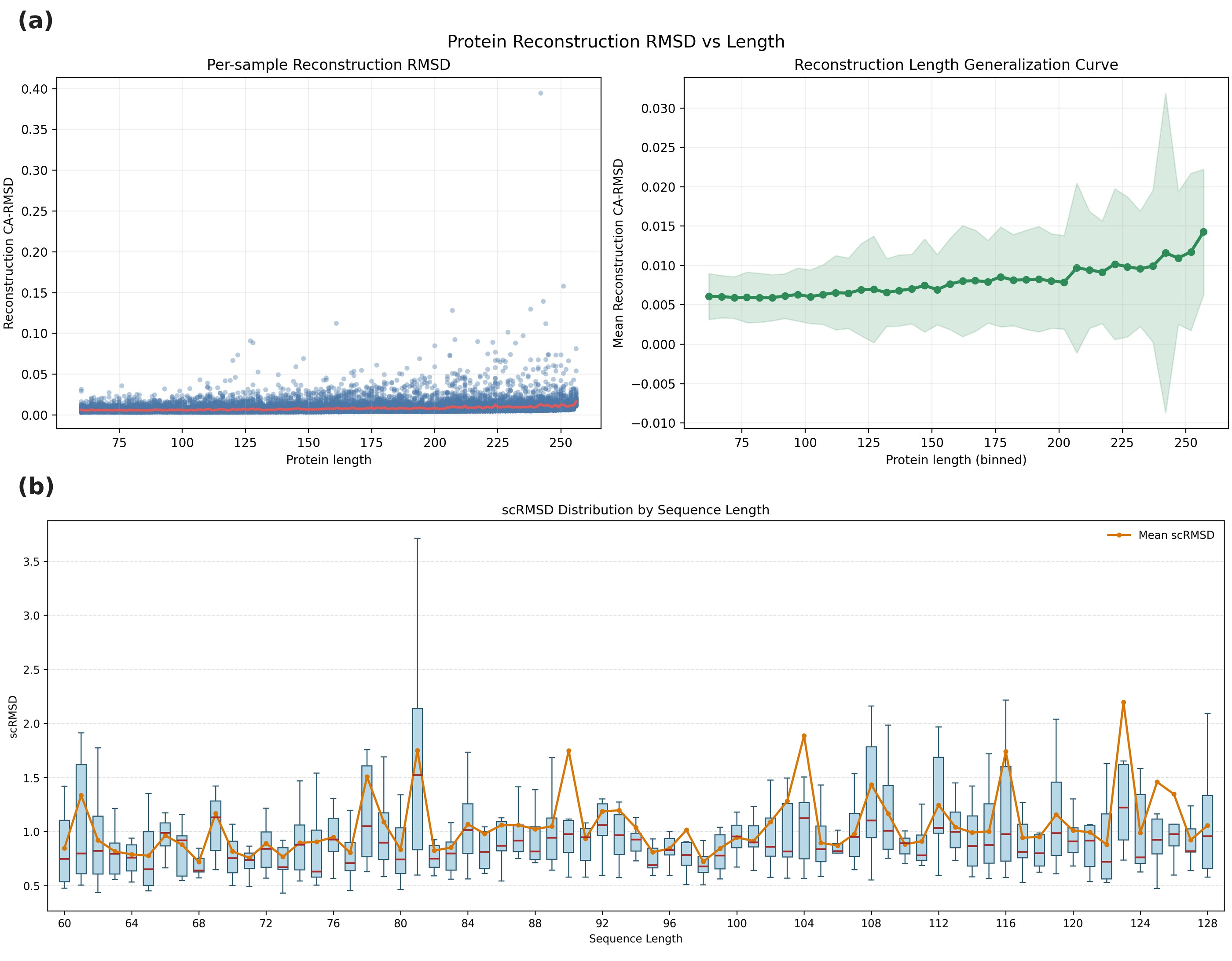
Figure 9 examines whether the SinAE protein model, trained with chains truncated to a maximum of \(256\) residues, generalises to longer chains and to generation lengths it was
never explicitly conditioned on. Figure 9 (a) plots per-sample reconstruction CA-RMSD against protein length on AFDB-FS; the binned mean (right panel) stays below \(0.015\) Å across the full
\(60\)–\(260\) residue range, increasing only mildly from \(\sim 0.006\) Å at 60 residues to \(\sim 0.014\) Å at 260
residues. This sub-linear scaling indicates that the flow-matching decoder does not require length-conditioned training to remain accurate on longer chains. Figure 9 (b) reports the analogous picture on the generative side:
the distribution of self-consistency scRMSD as a function of generated length. The mean scRMSD remains in a narrow band between 60 and 128 residues without any monotonic upward trend; quantitative per-length numbers are reported in Table [tbl:tab:performance].
17 Protein Reconstruction: Full Table with \(\pm\)std↩︎
Table 4 reproduces the protein-backbone reconstruction RMSD numbers from Table 2 with the full mean\(\,\pm\,\)std.uncertainties from ProteinBench [42].
| CASP14 | CASP15 | ||||
|---|---|---|---|---|---|
| 2-4 (lr)5-6 Method | T | T-dom | oligo | TS-dom | oligo |
| CHEAP | 11.16 \(\pm\) 10.09 | 4.71 \(\pm\) 5.21 | 11.10 \(\pm\) 11.95 | 10.98 \(\pm\) 12.44 | 8.24 \(\pm\) 14.12 |
| ESM3 VQ-VAE | 1.28 \(\pm\) 2.32 | 0.66 \(\pm\) 0.42 | 3.11 \(\pm\) 7.41 | 1.25 \(\pm\) 1.28 | 2.47 \(\pm\) 2.27 |
| DPLM-2\(^{*}\) | 1.94 \(\pm\) 1.99 | 1.47 \(\pm\) 0.42 | 3.81 \(\pm\) 7.20 | 4.58 \(\pm\) 6.62 | 3.83 \(\pm\) 6.90 |
| ProteinAE | 0.51 \(\pm\) 1.56 | 0.23 \(\pm\) 0.11 | 0.31 \(\pm\) 0.27 | 0.31 \(\pm\) 0.21 | 0.43 \(\pm\) 0.51 |
| 0.010 \(\pm\) 0.005 | 0.011 \(\pm\) 0.004 | 0.013 \(\pm\) 0.008 | 0.013 \(\pm\) 0.009 | 0.014 \(\pm\) 0.005 | |
4pt
18 Material Generation: Full MP-20 Breakdown↩︎
Table 5 reports the complete MP-20 generation breakdown, including the Overall validity column (\(\mathrm{Overall}=\mathrm{Structure}\times\mathrm{Composition}\), which is derivable from the main-text table) and the Metastable rate (\(E_{\mathrm{hull}}{<}0.1\) eV/atom). Both columns are omitted from the main paper because Overall is redundant and Metastable rate is the input to the M.S.U.N.metric that we already report.
| Validity Rate | Metastable | Stable | M.S.U.N. | S.U.N. | |||
| Model | Structure | Composition | Overall | rate | rate | rate | rate |
| CDVAE | 100.00 | 86.70 | – | – | 1.6 | – | – |
| DiffCSP | 100.00 | 83.25 | – | – | 5.0 | – | 3.3 |
| UniMat | 97.2 | 89.4 | – | – | – | – | – |
| FlowMM | 96.85 | 83.19 | 80.30 | 30.6 | 4.6 | 22.5 | 2.8 |
| FlowLLM | 99.94 | 90.84 | 90.81 | 66.9 | 13.9 | 26.3 | 4.7 |
| Jointly-trained ADiT | 99.74 | 92.14 | 91.92 | 81.0 | 15.4 | 28.2 | 5.3 |
| (MP20-only) | 98.29 | 88.89 | 88.40 | 79.6 | 14.1 | 24.3 | 4.6 |
| (joint) | 99.29 | 90.49 | 90.02 | 83.0 | 15.8 | 30.2 | 5.4 |
5pt
19 Molecule Generation: Per-PoseBusters-Check Breakdown↩︎
Table 6 reports the per-check pass rates for each of the seven PoseBusters sanity checks [44] for SinAE on QM9 (joint model) and GEOM-Drugs (\(10\) k samples each), together with the aggregate PB Valid rate (passes all seven checks) reported in
Tables ¿tbl:tab:gen95mol95qm9?–[tbl:tab:gen95mol95geom]. The breakdown shows that on QM9 the residual is dominated by the internal
energy check (\(96.8\%\)), and on GEOM-Drugs by internal steric clash (\(96.7\%\)) and bond angles (\(97.8\%\)); other checks are at
or near \(100\%\).
| Test (% pass) | (QM9, joint) | (GEOM-Drugs) |
|---|---|---|
| All atoms connected | 100.00 | 99.48 |
| Bond lengths | 99.59 | 99.07 |
| Bond angles | 100.00 | 97.84 |
| No internal steric clash | 99.90 | 96.70 |
| Aromatic ring flatness | 100.00 | 100.00 |
| Double bond flatness | 99.90 | 99.90 |
| Reasonable internal energy | 96.83 | 98.45 |
| PoseBusters Valid (all 7) | 96.52 | 92.58 |
6pt
20 MOF Generation: Full MOFChecker Sanity Checks↩︎
Table 7 reports the full set of MOFChecker sanity checks for 1,000 unconditionally sampled MOF structures from SinAE (trained on QMOF) and the jointly-trained ADiT baseline. The main text reports MOF
reconstruction in Table ¿tbl:tab:recon95nonprot?; this appendix provides the generation-side comparison. SinAE outperforms ADiT by \(+6.1\) points on the aggregate validity rate (\(16.28\%\) vs \(10.2\%\)), with consistent improvements on nearly every individual sanity check.
| Test (%) | Joint ADiT | |
|---|---|---|
| Has carbon \(\uparrow\) | 100.0 | 100.0 |
| Has hydrogen \(\uparrow\) | 99.8 | 100.0 |
| Has atomic overlap \(\downarrow\) | 5.2 | 10.8 |
| Has overcoord.C \(\downarrow\) | 12.8 | 34.3 |
| Has overcoord.N \(\downarrow\) | 0.4 | 1.6 |
| Has overcoord.H \(\downarrow\) | 1.3 | 3.6 |
| Has undercoord.C \(\downarrow\) | 39.2 | 72.1 |
| Has undercoord.N \(\downarrow\) | 26.9 | 39.9 |
| Has undercoord.rare earth \(\downarrow\) | 0.2 | 0.8 |
| Has metal \(\uparrow\) | 100.0 | 99.4 |
| Has lone molecule \(\downarrow\) | 49.8 | 83.2 |
| Has high charge \(\downarrow\) | 0.2 | 2.5 |
| Has suspicious terminal oxo \(\downarrow\) | 3.1 | 5.8 |
| Has undercoord.alkali \(\downarrow\) | 0.7 | 6.4 |
| Has geom.exposed metal \(\downarrow\) | 4.0 | 9.6 |
| Validity rate (all passed) \(\uparrow\) | 16.28 | 10.2 |
21 Generated Sample Visualisations↩︎
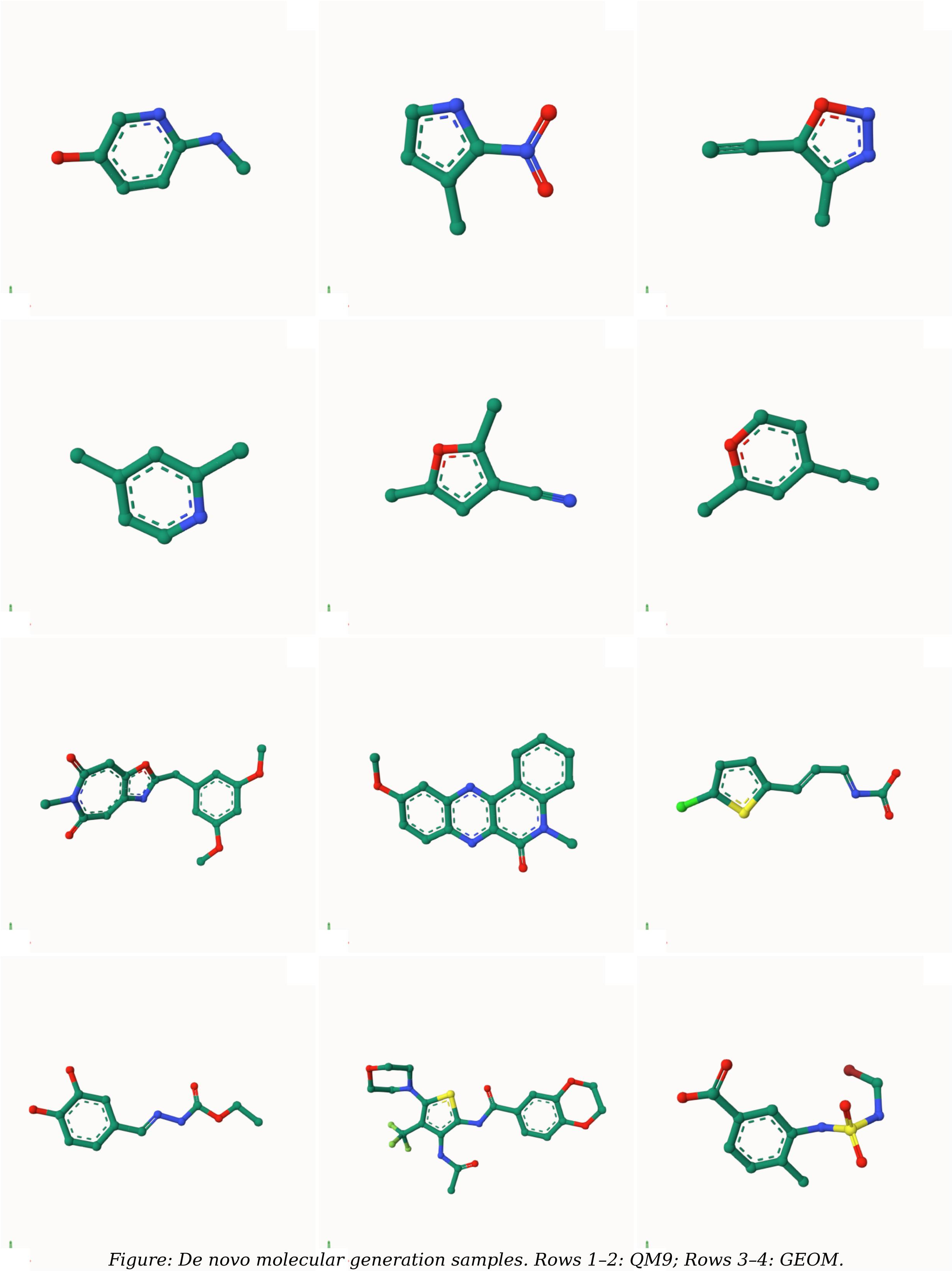
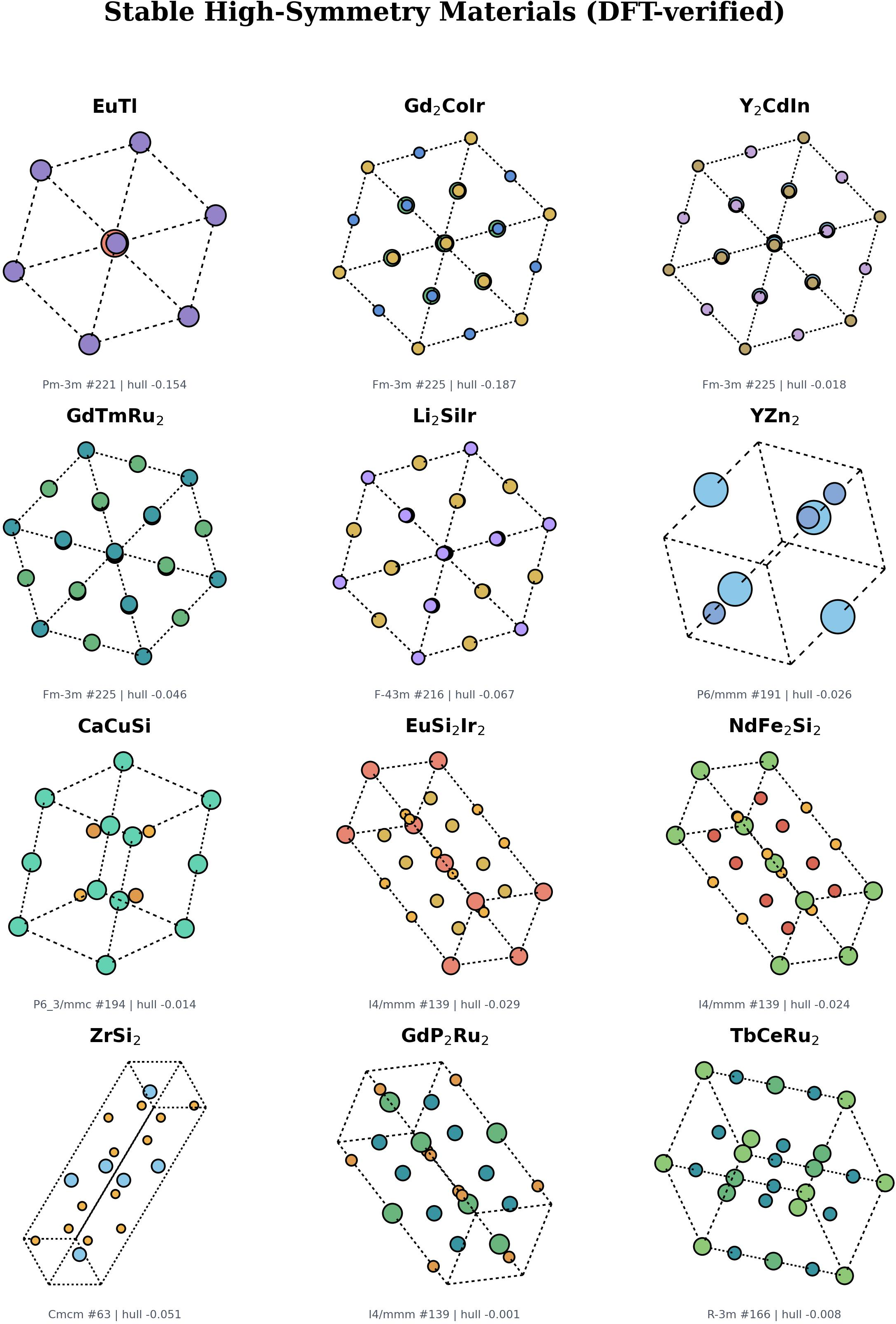
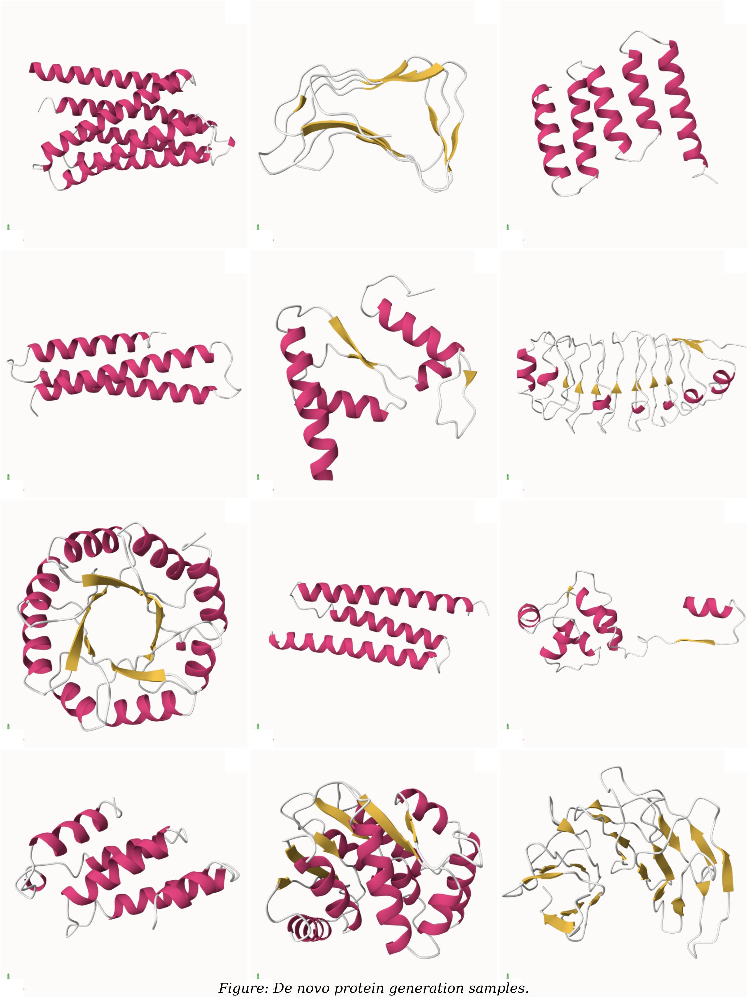
Figures 10–12 show unconditional samples drawn from the latent DiT prior of SinAE across all evaluated domains (QM9 small molecules, GEOM-Drugs drug-like molecules,
MP-20 crystals, and AFDB-FS proteins), decoded with the corresponding flow-matching decoder. Samples are uncurated unless otherwise stated.