: Computer Architecture Simulation as a Service
July 14, 2026
Abstract
Conducting a complete computer architecture simulation study is challenging because configuration, execution, and analysis are often encoded implicitly in scripts or directory conventions rather than represented explicitly. As a result, studies are difficult to scale, hard to reproduce, and dependent on custom tooling at every stage. We present ArchSim, which makes the structure of a simulation study explicit. In ArchSim, hardware topologies are described as declarative graphs that automatically generate executable simulation code, eliminating hand-written simulator programs. Stateless runners autonomously claim and execute jobs from a shared experiment store, enabling configuration-benchmark matrices to scale without manual orchestration. Simulation outputs are stored as structured artifacts tied to configurations, benchmarks, and hardware components, enabling systematic result exploration without custom parsers. We evaluate ArchSim on a \(12 \times 8 = 96\)-configuration simulation matrix spanning memory-bound, compute-bound, and mixed-intensity GPU workloads. Declarative simulation specifications drive full simulations with a median kernel time error of 0.18% relative to hand-written MGPUSim configurations across 95.8% of configurations. The platform introduces only 1.6 seconds of overhead per simulation, negligible relative to realistic simulation workloads.
1 Introduction↩︎
Simulation is central to computer architecture research. Building physical prototypes for each design is prohibitively expensive, so researchers rely on simulation to explore design choices and evaluate architectural ideas before hardware is built [1]. Simulators such as gem5 [2], [3], SST [4], Multi2Sim [5], AccelSim [6] and MGPUSim [7] have become foundational infrastructure for the field. As architectural designs grow more complex, they incorporate heterogeneous accelerators, deep memory hierarchies, and increasingly large software stacks. As a result, simulation studies now explore larger design spaces and require executing thousands of simulations across many configurations and benchmarks.
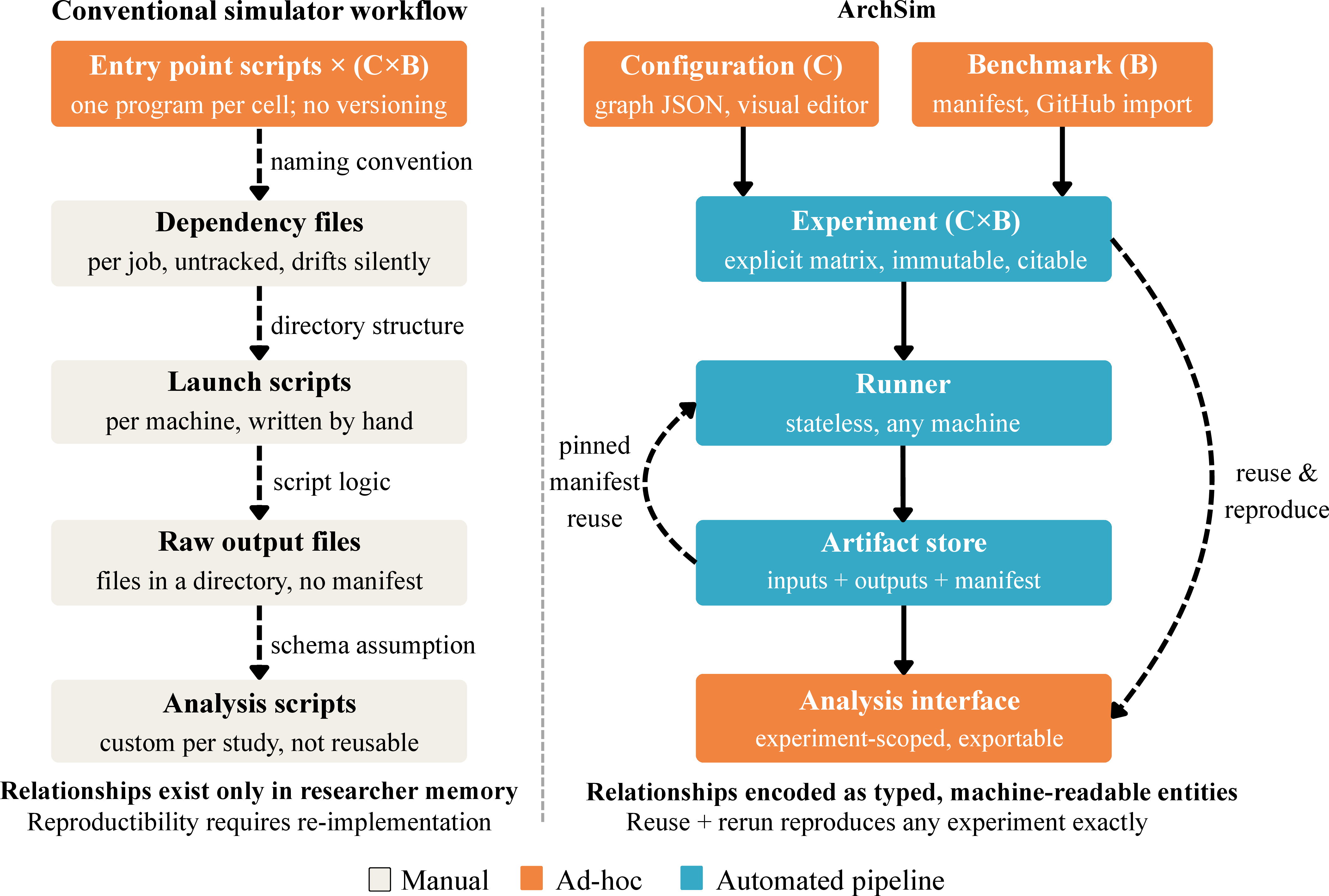
Despite the maturity of individual simulators, the barrier to conducting a complete simulation study remains high. In current practice, researchers define hardware configurations as imperative simulator source code rather than declarative specifications, orchestrate execution through hand-written, all tied together through naming conventions and directory structures. This approach introduces four primary barriers:
Configuration complexity. Hardware topologies are expressed as imperative simulator source code that instantiates dozens of components, binds typed ports, and wires components together in dependency order. Any change to the topology requires manually updating every affected line across every configuration variant, with no structural check that the result is consistent [2], [7].
Environment setup. Executing a study across multiple machines requires per-machine installation of the correct toolchain, fetching of simulator and benchmark repositories, and writing orchestration scripts that encode the simulation structure in shell logic and directory naming, with no portable description of the execution environment.
Simulation extensibility and scalability. Adding a new configuration means updating every script, directory, and aggregation pipeline that references the simulation structure by name. As the number of configurations and benchmarks grows, this fragility compounds: a study with \(C\) configurations and \(B\) benchmarks requires maintaining \(C \times B\) simulation programs with no structured representation of the simulation as a whole. Because relationships between configurations, benchmarks, and outputs are encoded only in naming conventions and script logic, inconsistencies are difficult to detect in practice [8].
Result interpretability. Analyzing results requires custom parsing scripts tightly coupled to the simulator output format and directory layout. Because simulation metrics are spatially organized across hardware components, flat parsing scripts cannot represent this structure, making it difficult to trace a performance observation back to the specific component that caused it [2], [7].
Simulation study in computer architecture is not just a simulator run. It is a structured scientific experiment consisting of hardware configurations, benchmarks, a systematic execution of every configuration-benchmark pair, and analysis that draws conclusions from the resulting data. The four barriers above share a common root cause: the structure of the experiment is encoded in code, scripts, and directory conventions rather than being represented explicitly. When configuration is code, it cannot be validated, stored, or re-executed without the original developer’s environment. When execution is orchestrated by scripts, adding one configuration requires updating every artifact that encodes the experiment structure. When outputs are files in a directory, analysis requires custom parsers that break the moment the experiment changes. Making the structure of a simulation experiment explicit and machine-readable eliminates all four barriers systematically. Figure 1 illustrates this contrast between conventional script-based workflows and ArchSim’s explicit, structured representation of simulation experiments.
Prior work has addressed individual pieces of this problem. Existing simulators provide detailed hardware models but leave simulation structure encoded in the scripts and directory conventions that surround them, with no platform-level support for managing configurations, benchmarks, or results as structured entities. Workflow management systems such as MLflow [9] and ReproZip [10] address reproducibility for flat parameter spaces but do not represent hardware topology graphs, typed port bindings, or configuration-benchmark matrices.
We introduce ArchSim, a web-based simulation experiment platform for computer architecture research that addresses each of the four barriers directly. To eliminate configuration complexity, ArchSim provides a visual flow editor where researchers build hardware topologies by placing component nodes on a canvas, setting parameters, and connecting ports, with no simulator source code written or maintained. ArchSim automatically generates a complete, correct simulation program from the graph. To remove environment setup overhead, we introduce a runner that handles toolchain setup, code generation, compilation, and execution automatically on any registered machine. To scale experiments without manual orchestration, ArchSim materializes the full \(C \times B\) simulation matrix and queues all jobs automatically, showing live per-cell status as simulations complete. To make results interpretable without custom scripts, ArchSim provides comparative views of simulation results with component-level drill-downs for deeper analysis.
ArchSim aims to simplify and formalize the end-to-end workflow of architecture simulation studies. This paper makes the following contributions:
An explicit experiment model that formalizes configurations, benchmarks, and experiments as first-class machine-readable entities, enabling experiments to be reproduced directly from their stored representation without reconstructing scripts or directory layouts.
A declarative configuration representation and automatic code generation pipeline that allows hardware topologies to be described as structured graphs rather than hand-written simulator programs, and automatically translates these descriptions into executable simulation code.
A distributed execution model in which stateless runners claim and execute simulation jobs autonomously from a shared experiment store, enabling large configuration-benchmark matrices to be explored without manual orchestration.
A structured analysis interface that records simulation outputs as structured artifacts tied to configurations, benchmarks, and hardware components, supporting systematic metric comparison and interactive result exploration without custom parsing scripts.
2 Design Requirements↩︎
The artifacts that define an experiment are rarely captured explicitly and often exist only in the researcher’s mental model of the experiment. Consider a simulation study that sweeps five cache configurations across six benchmarks. A pattern of fragility appears across architecture simulators: gem5 uses Python scripts to instantiate and connect simulation objects, SST uses similar programmatic configuration, and MGPUSim uses Go source programs. In each case, hardware configurations are expressed as imperative code, so each configuration variant requires a separate program or script.
We use MGPUSim to illustrate a concrete instance of this problem. A 5 \(\times\) 6 experiment requires maintaining 30 separate simulation programs along with benchmark inputs, output files, and analysis scripts linked together through naming conventions and directory structures. As the number of configurations and benchmarks grows, the resulting workflow becomes increasingly fragile: small changes require editing many programs, mistakes propagate silently across runs, and reproducing results requires reconstructing the entire artifact graph.
R-1: Configuration and Code Generation. Defining the hardware system to simulate is the first and most technically demanding stage of a simulation experiment. A typical architecture topology may include cores, cache hierarchies, address translation structures such as TLBs, memory controllers, and interconnect components [2], [6], [7]. In current practice, topologies are expressed as simulator source code, making component relationships invisible to the user and impossible to validate without executing the program. The most time-consuming errors in hand-written simulator workflows are not logical mistakes but silent wiring faults: missing port bindings that compile without error yet produce zero-metric outputs. Identifying such faults requires reading binary output, cross-referencing it with source, and manually tracing the component graph across dozens of components and hundreds of port bindings. Researchers should be able to define hardware topologies through a structured visual interface that validates wiring at definition time, and the system should automatically generate correct executable simulation code from that definition, eliminating hand-written simulator programs entirely.
R-2: Execution and Scalability. After a configuration is developed and verified, researchers evaluate the design by running benchmarks against it. A study with \(C\) configurations and \(B\) benchmarks requires \(C \times B\) compiled simulation programs, each needing separate compilation, job scripts, and result aggregation logic. Adding a new configuration requires updating job scripts, file naming schemes, and aggregation pipelines by hand, with no structured representation of the experiment as a whole. Researchers should be able to easily run large configuration-benchmark matrices across multiple machines, with simulations scaling out automatically as more machines designs are added.
R-3: Reproducibility. Reproducing a simulation experiment in practice is rarely achieved. The inputs required to reproduce a run, hardware configuration, benchmark parameters, simulation seed, and metric extraction scripts, are scattered across simulator source files and ad hoc pipelines, making reproduction dependent on incomplete documentation or direct communication with the original authors [8]. Even when inputs are preserved, simulator version drift can silently alter results between runs, yet the exact dependency versions used are rarely recorded. Every simulation run should store its complete input specification and resolved simulator dependency versions in a structured, machine-readable format sufficient to reproduce the run.
R-4: Result Analysis. Architecture simulation produces large volumes of performance data organized across many hardware components. Understanding performance requires comparing results across configurations and benchmarks while also examining component-level behavior such as cache hit rates or CPI stack breakdowns. In conventional workflows this analysis is performed using custom scripts tightly coupled to the simulator output format and the experiment directory structure. When the experiment changes, these scripts must be updated manually, and because the relationship between outputs and analysis logic is encoded only in script logic, there is no mechanism to ensure consistency. Simulation outputs should be stored in a structured, queryable format alongside their input specifications, and researchers should be able to retrieve experiment-level metrics and navigate to component-level details for any selected configuration and benchmark without writing custom parsing scripts.
3 ArchSim↩︎
We first introduce the core concepts and entities that ArchSim uses to represent an experiment (Section 3.1), then describe how each design decision satisfies the requirements identified in Section 2. ArchSim organizes the workflow of a simulation study as a sequence of explicit stages spanning configuration, execution, reproducibility, and analysis.
3.1 Organization↩︎
ArchSim organizes the end-to-end workflow of an experiment study into four areas: Model, Configuration, Experiment, and Analysis (see Figure 4). Researchers first populate the Model library with reusable hardware component definitions and benchmark workloads imported from external repositories. They then use the Configuration editor to assemble those components into complete hardware topologies, described as declarative graphs and stored as JSON documents. Next, an Experiment combines a set of configurations and benchmarks into a \(C \times B\) simulation matrix, dispatches all jobs to registered runners, and displays live per-cell status as simulations complete. Finally, the Analysis view queries the resulting artifact store to compare metrics across the matrix and drill down into component-level behavior for any selected (configuration, benchmark) pair.
Each area is built around a set of first-class entities that explicitly capture the structure of an experiment. The Model area organizes reusable component definitions and benchmark workloads as typed, machine-readable objects. The Configuration area represents hardware topologies as declarative graphs of model instances, parameters, and port connections, and automatically generates executable simulation code from them (Section 3.2). The Experiment area manages the \(C \times B\) simulation matrix, dispatching jobs to stateless runners and preserving complete input and version information for reproducibility (Sections 3.3 and 3.4). The Analysis area stores simulation outputs as structured artifacts tied to configurations, benchmarks, and hardware components, supporting systematic metric comparison without custom parsing scripts (Section 3.5). Figure 2 shows how these entities interact across the experiment lifecycle, and the following subsections describe each in detail.

Model. A model encapsulates the behavior of a single architectural component such as a cache, TLB, compute unit, memory controller, or interconnect. We currently support Akita [11] simulation engine given is high flexibility and simpler interface. We are working on supporting gem5 [2] and SST [4] with an adaptor using CGO [12], a tool that bridges Go and C code.
Benchmark. A benchmark represents a workload that executes on the simulated hardware. Like models, benchmarks are imported from external repositories and described by a manifest that declares the workload’s parameters and builder package. A benchmark definition is shared across all experiments and configurations that reference it, so the same workload can be evaluated across many hardware configurations without duplication.
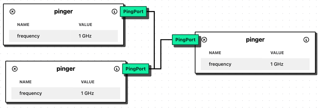
Configuration. A configuration defines how hardware models are instantiated, parameterized, and connected to form a complete simulated hardware system. ArchSim represents configurations as graphs, where nodes correspond to hardware models and edges represent interconnections between them (Section 3.2). A flow editor provides a graphical interface for constructing and modifying configurations without writing simulator code, as shown in Figure 3 (satisfying R-1).
Experiment. An experiment represents a systematic evaluation as an explicit \(C \times B\) matrix of configurations and benchmarks. To create an experiment, a researcher selects configurations and benchmarks from their saved definitions. ArchSim immediately renders the full \(C \times B\) grid, where each cell corresponds to one (configuration, benchmark) pair to be simulated, as shown in Figure 4. When the experiment is launched, ArchSim materializes one simulation record per cell. Each record contains a complete, self-contained job specification including the hardware configuration, benchmark parameters, simulation seed, and trace settings, assembled from the current state of the selected configurations and benchmarks at launch time. The specification is stored immutably so that subsequent edits to a configuration or benchmark do not silently alter queued or in-progress simulations. The experiment grid reflects the live status of all simulations, giving researchers a unified view of progress across the entire experiment matrix.
Simulation. A simulation corresponds to a single \((\textit{configuration}, \textit{benchmark})\) pair in the experiment matrix and represents the logical unit of work scheduled by the system. Each
simulation progresses through a lifecycle Ready \(\rightarrow\) Running \(\rightarrow\) [Done | Failed | Canceled]. The
resolved simulator dependency versions are recorded after the first successful run in an experiment and reused for all subsequent runs, allowing ArchSim to manage retries and track reproducibility metadata without modifying the logical structure of the
experiment.
Runner. A runner is any machine registered to an ArchSim account that can claim and execute simulation jobs on behalf of a researcher. Once registered, a machine launches the archsim-runner daemon via the CLI, which
continuously polls the backend for pending jobs, claims work autonomously, executes the simulation pipeline, and reports results. Runners are classified as shared or personal. Shared runners are available to all platform users and are
centrally managed by an institution or administrator. Personal runners are registered by an individual researcher and are accessible only to that user. Researchers can attach private machines such as workstations or lab servers as personal runners for
their own simulations. Each runner polls the backend for pending jobs, claims work autonomously, executes the simulation pipeline, and reports results. All job-specific information is included in the payload, so simulations can execute on runners without
manual configuration (satisfying R-2). The runner is also responsible for translating the declarative configuration JSON into an executable simulation program; this code generation pipeline is described in detail in Section 3.2.
Analysis. ArchSim provides a structured analysis interface that queries the artifact store generated during simulation execution. At the experiment level, the system retrieves summary metrics across all simulations from the Postgres database (satisfying R-4). At the simulation level, the interface supports component-level drill-down for a selected \((\textit{benchmark}, \textit{configuration})\) pair (satisfying R-4). Raw simulation artifacts may also be stored in S3 for deeper post hoc analysis (Section 3.4).
3.2 Declarative Configuration and Code Generation↩︎
Architecture simulators typically construct hardware systems by writing configuration files (e.g., Multi2Sim) or programs (e.g., gem5, MGPUSim) that instantiate components and connect ports through builder APIs. This couples experiment configuration with simulator source code, making it difficult to generate and manage large families of hardware configurations for systematic architectural studies.
ArchSim addresses this by representing hardware topologies as declarative configuration graphs that define the simulation to be generated (addressing R-1). The hardware structure is described as a structured document specifying component instances, parameters, and interconnections, allowing the system to automatically generate executable simulation programs without researcher-authored code.
Configuration representation. Configurations are defined through a graphical flow editor where researchers place component nodes, set parameters, and draw port connections between components. The resulting topology is serialized into a
JSON document by ArchSim. Nodes represent component instances, each with a name, a builder_package identifying the builder to invoke, and a params list of parameter assignments. A builder is a factory module whose
construction API instantiates a component class; it is identified by its import path, which the code generation pipeline uses to invoke the correct constructor when assembling the executable simulation program. Parameter values may be literals, variable
references resolved during code generation, or structured port bindings referencing another component and port. Edges carry a name and a list of plugs identifying the component-port pairs to connect. Together, nodes and edges form
a directed graph that is validated before code generation: the runner checks that all port bindings and plugs reference existing components, verifies that referenced variables are defined, and confirms that the dependency graph contains no cycles. These
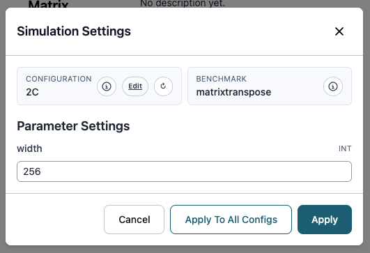
checks catch structural errors such as dangling references and circular dependencies at definition time rather than at compile time or simulation runtime. Benchmark-level parameters (Figure 5), are set
separately at experiment launch time and serialized into the simulation job when the researcher clicks Run Simulations, as shown in Figure 4.
Configuration space. The configuration abstraction supports four categories of architectural parameters, all expressible as declarative JSON edits without modifying simulator source code: component topology (adding, removing, or rewiring components in the graph), memory hierarchy (cache capacity, associativity, and block size), compute unit microarchitecture (pipeline width and subsystem parameters), and address translation and memory control (TLB structure and memory controller arrangement). Section 5 demonstrates this directly across all four categories.
Code generation pipeline. Given a configuration JSON and a benchmark manifest, the runner generates a complete simulation program, compiles it, and executes it automatically, producing structured performance metrics and optional trace artifacts for tools such as Daisen [13] (satisfying R-1). ArchSim does not modify the simulator core; instead, the runner synthesizes a self-contained host program that imports the existing simulator component libraries and benchmark packages and invokes their public builder APIs. The only requirement from the simulator libraries is the stable builder-style construction APIs they already expose.
The generation pipeline proceeds in five steps. First, the configuration JSON is parsed into an internal graph representation. Second, the graph is validated for structural correctness, checking component references, variable definitions, and dependency cycles. Third, the runner emits a Go source file containing the simulation engine initialization, topologically ordered component builder calls, port connection wiring, benchmark setup, and optional trace instrumentation. Fourth, module dependencies are resolved using the experiment’s pinned version manifest. Fifth, the program is compiled and executed, and the resulting metrics and artifacts are uploaded to the artifact store.
Because these translation steps follow a fixed set of rules, the generated program is a deterministic function of the configuration JSON and benchmark parameters, so storing the configuration is sufficient to reproduce the exact simulation program used in any experiment. The same pipeline applies regardless of whether edits change only parameter values or also add and remove nodes and edges.
3.3 Pull-Based Distributed Execution↩︎
ArchSim addresses R-2 through a pull-based distributed model in which stateless runners claim self-contained jobs from a shared backend queue. Because the job payload is complete, containing the configuration JSON, benchmark parameters,
simulation seed, and pinned version manifest, any machine running the archsim-runner CLI can join the execution pool and begin executing simulations without prior simulator installation or manual environment configuration.
Job lifecycle. When a researcher clicks Run Simulations, as shown in Figure 4, the backend materializes one simulation record per cell in the \(C
\times B\) matrix, each entering the Ready state. By default, re-running an experiment resets incomplete and failed cells to Ready with refreshed payloads; an incremental mode is also available that skips cells already
marked Done, allowing researchers to fill in only missing results.
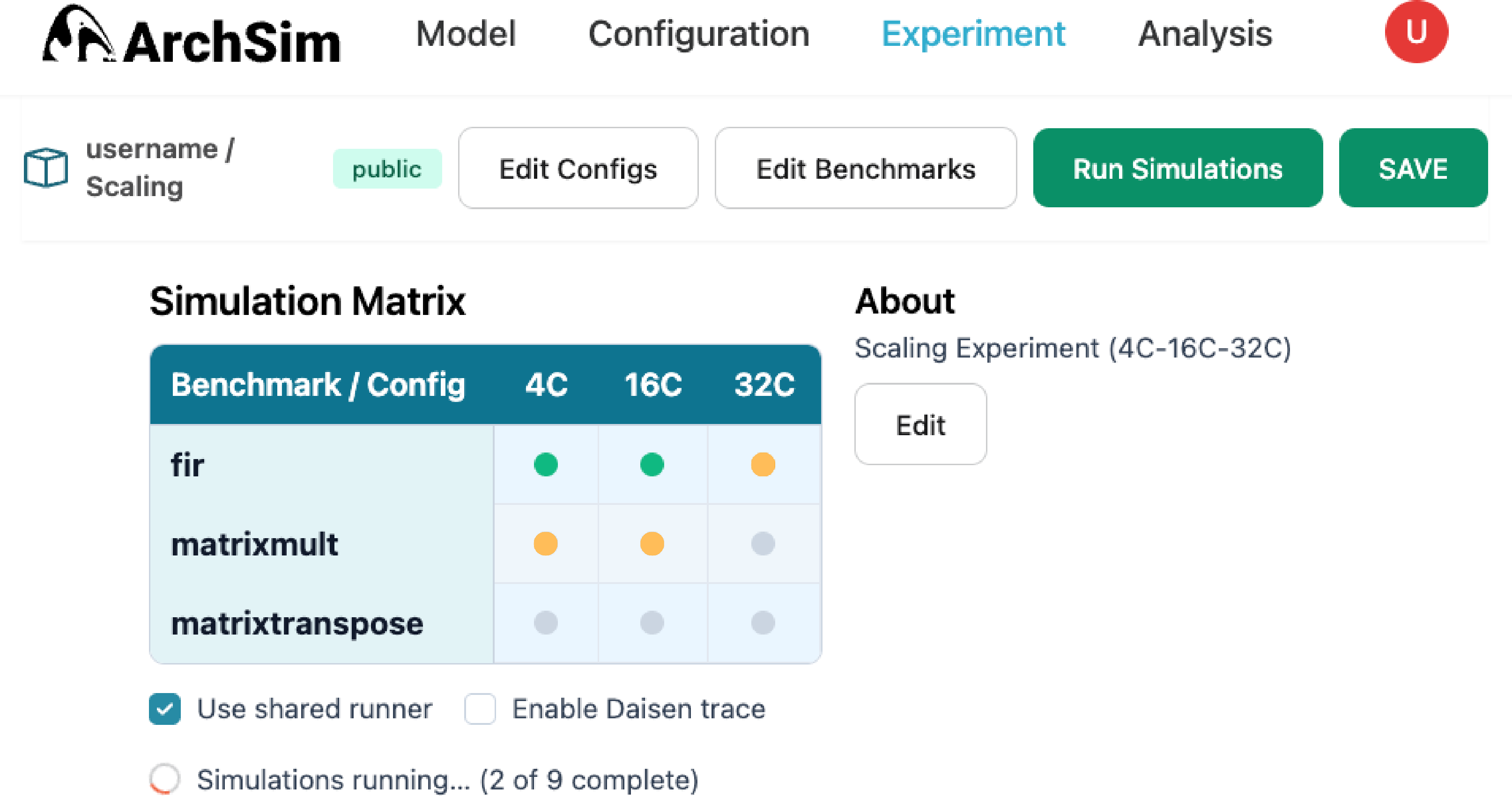
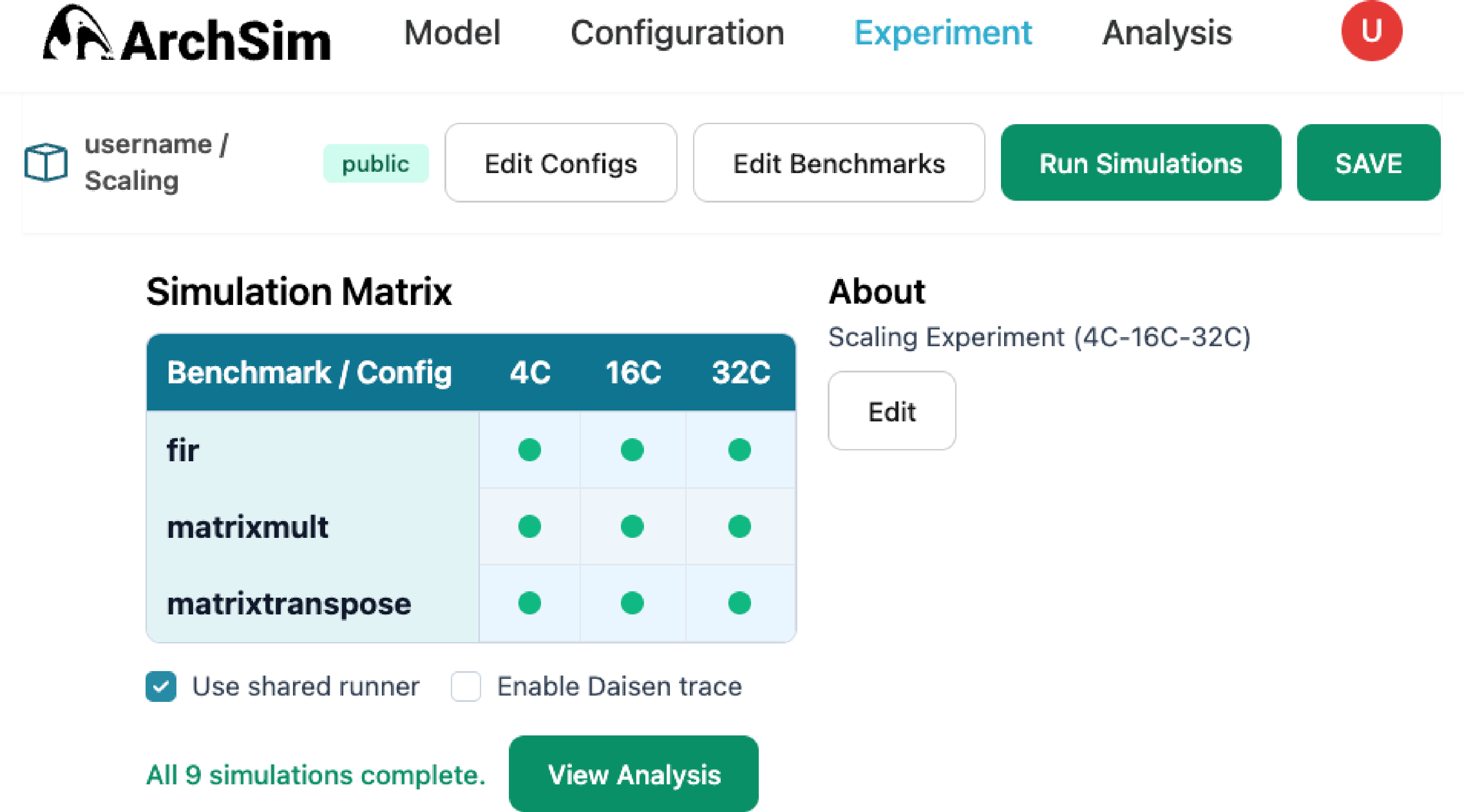
Figure 4: ArchSim experiment dashboard.. a — The simulation matrix during execution, showing per-cell status indicators for a 3-configuration \(\times\) 3-benchmark study. Configurations are ordered by CU count (4C, 16C, 32C) along the columns and benchmarks along the rows., b — The same dashboard after all 9 simulations have completed, with the View Analysis button enabled. Researchers can immediately identify failed cells and re-run the experiment after correcting errors without navigating away from the experiment view.
Runner execution. Runners periodically poll the backend for available jobs and claim work independently. Once a job is claimed, the runner generates the simulation program, compiles it, executes the benchmark, reports the result, and
uploads generated artifacts. Claim rules are enforced server-side, and jobs that remain Running beyond a timeout are reset to Ready and returned to the queue. The experiment dashboard (Figure 4) displays the full \(C \times B\) matrix with per-cell outcomes, allowing researchers to identify failed pairs and resubmit after correcting errors.
3.4 Reproducibility through Explicit Artifact Preservation↩︎
ArchSim ensures experiment reproducibility by explicitly preserving both the inputs and outputs of every simulation run. Instead of treating simulation programs, configuration parameters, and results as loosely connected files in a researcher’s working
directory, ArchSim records them as structured artifacts associated with each experiment. This design allows simulations to be reconstructed and re-executed directly from stored records on any machine running the archsim-runner CLI, independent
of the environment that originally queued the job.
Each queued simulation stores its complete job specification as a single JSON document containing both the hardware configuration and benchmark sections. The platform additionally persists relational identifiers (experiment, configuration, benchmark), run status, structured metrics, and optional large binary artifacts via storage URLs.
Complete input preservation. The platform retains the full input specification for each run; when a simulation completes, structured outputs are stored alongside it (addressing R-3). The stored record includes the hardware configuration document, benchmark definition and runtime parameters, and the simulation seed. Together these inputs are sufficient to regenerate the simulation program and re-execute the experiment. Because ArchSim’s code generation pipeline is deterministic, reconstructing a simulation from the stored configuration produces a program that is semantically equivalent to the original run for a given runner version.
Experiment-level version manifest. Preserving configuration inputs alone is insufficient if the underlying simulator evolves over time. ArchSim therefore records the exact simulator dependency versions used during execution (addressing
R-3). When the first simulation in an experiment completes successfully, the resolved Go module graph (go.mod and go.sum) is captured and stored as the version manifest for that experiment. All subsequent simulations in the
experiment reuse this manifest when claiming jobs, ensuring that every run executes against the same simulator versions even if upstream repositories change. This mechanism is automatic and requires no manual version management by the researcher. Pinning
versions at the experiment level ensures that all cells in the \(C \times B\) matrix execute against the same simulator build, so differences in results reflect only configuration and benchmark inputs rather than toolchain
variation.
Different experiments may use different simulator versions depending on when their first simulation completed. If no simulation in an experiment completes successfully before all runs fail, the manifest is not established and version pinning does not take effect for that experiment.
Structured output storage. Simulation outputs are stored in a relational schema: each metric row is keyed to the experiment, configuration, and benchmark that produced it, and each metric names the simulated hardware component it refers to using a hierarchical component path in the simulator’s naming scheme (addressing R-3). This enables systematic comparison across the experiment matrix without custom parsing scripts, since results can be grouped by configuration or benchmark, directly from the store. Raw simulation artifacts may also be stored for deeper post hoc analysis when needed.
3.5 Result Analysis↩︎
ArchSim provides a result analysis feature that operates directly on the structured artifact store produced during simulation execution. Because each metric is associated with its experiment and (configuration, benchmark) cell, and tagged with a
component path in the simulators’s metric schema, the interface supports both simulation comparisons and per-component inspection without custom parsing scripts. The interface renders a bar chart of a selected metric (e.g., kernel_time) across
all \(C \times B\) pairs, supporting grouping by configuration or benchmark to reflect the two standard axes of comparison in simulation studies: architectural design alternatives and workload characteristics. Users can
drill down through the component hierarchy to inspect component-level metrics and distributional summaries for any selected (configuration, benchmark) pair. For reproducible figures, the interface exports standalone Python scripts with embedded tabular
data, allowing plots to be regenerated and restyled for publication. Analysis beyond what the structured artifact store exposes, such as fine-grained execution traces, is supported through integration with tools such as Daisen [13].
Experiment-scoped metric retrieval. The interface retrieves all simulation runs belonging to a selected experiment and renders a bar chart comparison view across the \(C \times B\)
configuration-benchmark matrix for a selected metric, for example, simulated execution time (addressing R-4). Each bar corresponds to a stored metric value for a specific (configuration, benchmark) pair, letting researchers visually
identify best- and worst-performing configurations at a glance. Results can be grouped by configuration or by benchmark, enabling quick comparison of architectural alternatives or workload behaviors across the experiment without intermediate aggregation
pipelines, as shown in Figure 10 (a).
Component-level drill-down. Selecting a specific (configuration, benchmark) pair opens a component-level view derived from the stored metric locations (addressing R-4). Components are organized hierarchically
according to the simulator’s hardware structure, enabling navigation from experiment-level summaries to measurements collected at individual components such as compute units, caches, or memory controllers (Figure 10
(b)). For example, a researcher can inspect L2 read and write hit rates, L3 MSHR activity, or per-CU CPI stack contributions directly from this view, for any component that emits these counters, without writing any parsing scripts. Section 5 demonstrates this workflow concretely: an anomaly identified in the experiment-level bar chart is traced to near-zero L2 hit rates and nonzero L3 MSHR activity through the component-level drill-down.
4 Evaluation↩︎
We evaluate ArchSim across four studies: simulation accuracy (Section 4.2), which establishes that ArchSim-generated simulations are consistent with hand-written MGPUSim configurations; reproducibility (Section 4.3), which establishes that ArchSim introduces no additional non-determinism beyond the underlying simulator; runner scalability (Section 4.4), which evaluates the speedup delivered by the pull-based execution model as the number of concurrent runners grows; and execution overhead (Section 4.5), which characterizes the cost of ArchSim’s code generation and compilation pipeline relative to a pre-compiled baseline.
4.1 Methodology↩︎
Platform. Our experiments are conducted on a dual-socket AMD EPYC 7543 machine (64 cores, 128 hardware threads) with 251 GiB of main memory, running Ubuntu 22.04.5 LTS (kernel 5.15.0-173) and Go 1.26.1. All simulations are compiled and
executed by ArchSim runners registered on this machine. ArchSim’s record-and-reuse version manifest ensures that every simulation in each experiment uses identical akita and mgpusim dependency versions.
Simulation configuration. We integrate ArchSim with the MGPUSim simulator built on the Akita [11] simulation engine. Hardware configurations are defined declaratively in ArchSim’s flow editor as directed graphs of MGPUSim components. We evaluate eight CU configurations (1, 2, 4, 8, 16, 32, 64, 128 CUs) with all other topology parameters fixed. The CU sweep is chosen as the primary dimension because it exercises the code generation pipeline across a wide range of topology scales, from a single compute unit with a handful of components to a 128-CU system with hundreds of port bindings. The ArchSim configuration interface is not limited to this dimension: any parameter exposed by the MGPUSim builder API, including cache capacity, associativity, block size, interconnect bandwidth, TLB size, and memory controller count, can be modified through the flow editor’s parameter panel or swept across configurations without touching simulator source code. The case study in Section 5 demonstrates this directly: the four cache hierarchy configurations differ not only in the number of cache levels but also in associativity (4-way vs. 16-way), block size (64B vs. 128B), and the structural presence or absence of the L1.5 and L3 components, all expressed as declarative JSON changes. Each configuration is defined once in the flow editor and reused across all benchmarks and evaluation studies without modification.
Benchmarks. To ensure the robustness of our evaluation, we use 12 representative benchmarks drawn from five suites: AMDAPPSDK [14], HeteroMark [15], PolyBench [16], DNNMark [17], and Rodinia [18], covering the full range of GPU workload characteristics.
Benchmark parameters are listed in Table 1 and are held constant across both the accuracy and reproducibility studies.
| Abbrev. | Benchmark | Parameters |
|---|---|---|
| ATX | atax | \(512 \times 512\) |
| BiCG | bicg | \(512 \times 512\) |
| BTS | bitonicsort | length \(= 32{,}768\) |
| FWT | fastwalshtransform | length \(= 16{,}384\) |
| FIR | fir | length \(= 262{,}144\) |
| FW | floydwarshall | 512 nodes, 1 iteration |
| MM | matrixmult | \(128 \times 128 \times 128\) |
| MT | matrixtranspose | width \(= 2{,}048\) |
| NB | nbody | 4,096 particles, 3 iterations |
| NW | nw | length \(= 1{,}024\), penalty \(= 10\) |
| ReLU | relu | length \(= 4{,}194{,}304\) |
| SC | simpleconvolution | \(512 \times 512\), mask \(= 3\) |
Together, the 12 benchmarks and 8 CU configurations produce a \(12 \times 8 = 96\)-configuration experiment matrix that serves as the common evaluation substrate for simulation accuracy and reproducibility studies below.
4.2 Simulation Accuracy↩︎
We evaluate whether ArchSim-generated simulations produce results consistent with a reference MGPUSim implementation of the same platform topology. The reference implementation was written by hand using MGPUSim’s builder APIs directly, following the same process a researcher would use without ArchSim, and serves as the ground truth against which ArchSim’s code generation accuracy is measured. Both runners use identical component parameters, benchmark inputs, and simulation seed (seed \(= 0\)) under a serial discrete-event engine, eliminating all sources of non-determinism.
Figure 6 shows absolute relative error (RE) across all 96 configurations and Table 2 summarizes the results. 95.8% of configurations achieve RE \(<\) 5% and the median RE of 0.18% confirms the distribution is heavily concentrated near zero. Mean RE remains below 2% across all CU counts, reaching its lowest at 16 CUs (0.28%) and highest at 128 CUs (1.98%), indicating that the code generation pipeline handles structural translation correctly across topologies ranging from a single CU to 128 CUs.

| Metric | Value |
|---|---|
| Total configurations evaluated | 96 |
| Exact matches (RE \(<\) 0.005%) | 19 (19.8%) |
| Within 0.5% RE | 60 (62.5%) |
| Within 1% RE | 68 (70.8%) |
| Within 5% RE | 92 (95.8%) |
| Mean RE | 1.07% |
| Median RE | 0.18% |
| Maximum RE | 9.56% |
Accuracy varies by workload characteristic. The most accurate benchmarks are NB (mean RE 0.08%), BTS (0.11%), and NW (0.13%), whose execution is dominated by compute or regular memory access patterns. The least accurate are ATX (mean RE 2.73%), FW (2.38%), and BiCG (1.74%), which have irregular memory access patterns that produce cache-sensitive timing differences at higher CU counts. The four configurations exceeding 5% RE (SC at 2 CUs, ATAX at 32 and 64 CUs, BiCG at 32 CUs) all involve sub-millisecond absolute execution times where small absolute differences produce disproportionately large percentage errors; the absolute differences are architecturally insignificant.
4.3 Reproducibility↩︎
Simulator codebases evolve continuously, and even a minor internal change to a dependency can silently alter simulation outputs without any public API change or user warning. Without explicit version pinning, two researchers running the same experiment may silently execute against different simulator versions. ArchSim addresses this by recording a version manifest after the first successful run and reusing it for all subsequent runs in the experiment.
Version pinning is necessary and sufficient. We run the full 96-configuration simulation matrix under two conditions. Trial A uses ArchSim’s default pinned manifest, fixing all dependencies to exact versions
(mgpusim v4.2.0, akita v4.9.2). Trial B replaces mgpusim with a fork containing a single one-line change: doubling the vector memory transaction pipeline width in the compute unit builder. This change modifies no
public API and would be invisible to a user pulling the latest dependency version. Under Trial A, zero mismatches are observed across three trials and 288 total runs. Under Trial B, 8 of 96 configurations crash with verification failures and 66 of the
remaining 88 show measurable drift with a mean absolute deviation of 1.08% and a maximum of 14.66% (bicg at 16 CUs), with no user-visible warning. Version pinning is therefore both necessary and sufficient for reproducible simulation.
We next verify that ArchSim itself introduces no additional non-determinism beyond the underlying simulator when versions are pinned. We execute each of the 96 configurations three times under the same pinned version manifest, configuration JSON,
benchmark parameters, and seed. Figure 7 shows normalized kernel_time across three trials for twelve benchmarks spanning all CU counts.

ArchSim introduces no platform non-determinism. At 1 and 2 CUs, where the simulator runs serially, 9 of 12 benchmarks (75%) produce bit-identical kernel_time values across all three trials (CV = 0.00%). The exceptions show
variation attributable to floating-point operation ordering in their kernels, a simulator-level property independent of ArchSim. Any variation at higher CU counts is attributable entirely to the simulator’s parallel event ordering. Mean CV grows from 0.04%
at 2 CUs to 1.31% at 16 CUs, consistent with parallel discrete-event simulation behavior present in any MGPUSim runner. Overall, 83.3% of configurations achieve CV \(<\) 1% and 95.8% achieve CV \(<\) 5%. Averaging across three trials, mean RE against the baseline is 1.13% (median 0.30%), consistent with the single-run result from Section 4.2, confirming that inter-trial
variation is random noise with no directional component.
4.4 Runner Scalability↩︎
ArchSim’s pull-based execution model is designed to scale horizontally by adding runner processes that claim jobs autonomously from the shared queue without any centralized coordination. We evaluate whether this design delivers practical speedup as the number of concurrent runners grows.
We deploy 1, 2, 4, and 8 concurrent runner processes on the same host, each executing the archsim-runner binary independently. Runners poll the backend for pending jobs, claim work via a first-writer-wins database update, and report results
without communicating with each other. The job queue consists of 24 simulations (6 benchmarks \(\times\) 4 CU configurations: 1, 4, 16, and 64 CUs). We measure wall-clock time from the first job being claimed to the last
job reaching Done status and report speedup and parallel efficiency relative to the single-runner baseline.
Figure 8 shows the speedup curve against the ideal linear baseline, while Table 3 reports the efficiency trend across all runner configurations.
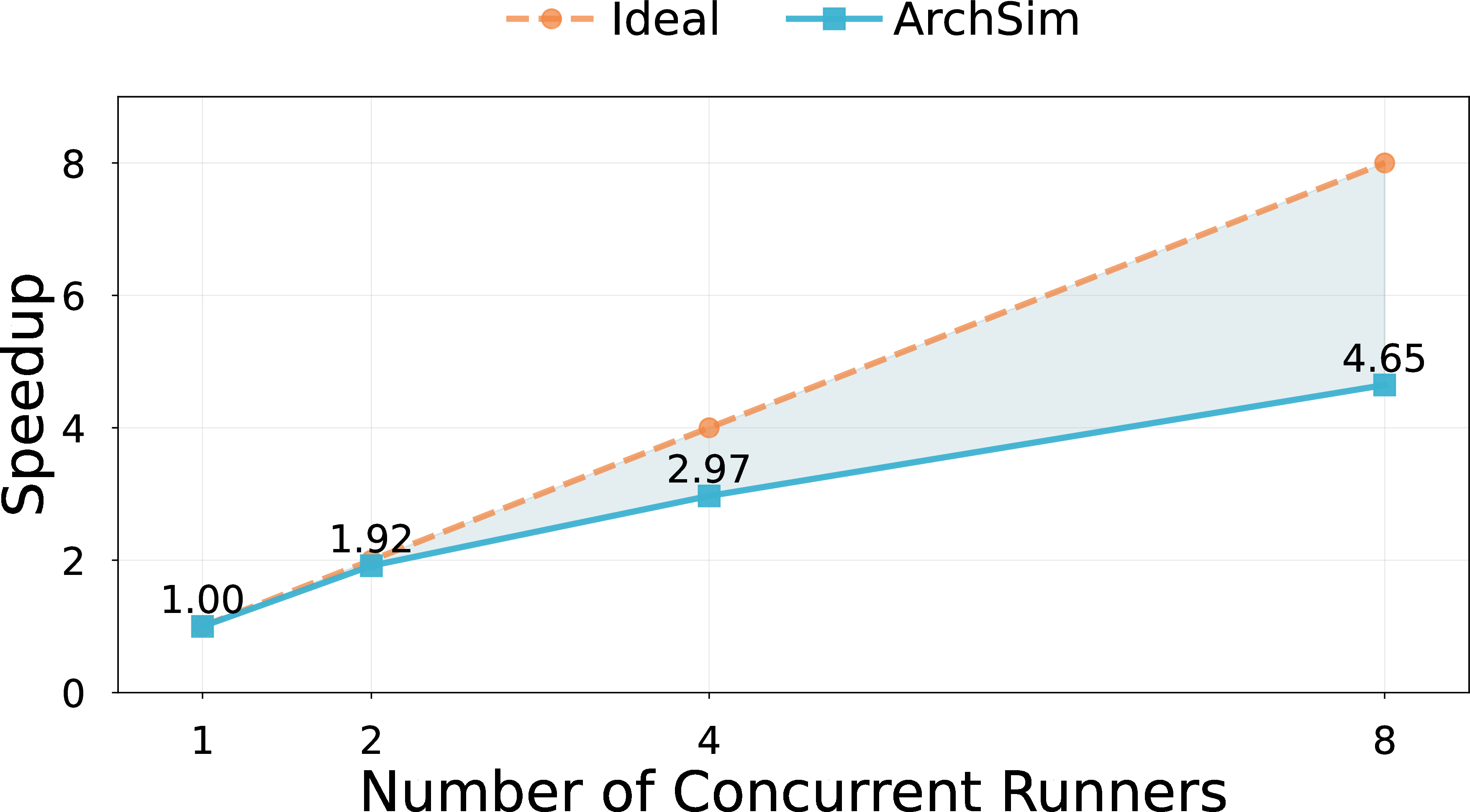
Speedup and wall-clock reduction. Table 3 summarizes the results. With 2 runners, ArchSim achieves 1.92\(\times\) speedup at 95.8% efficiency, confirming that the pull-based job claiming mechanism introduces negligible coordination overhead at low concurrency. With 4 runners, speedup reaches 2.97\(\times\) (74.3% efficiency), approaching the ideal 4\(\times\) and remaining well above the 70% threshold commonly used to characterize well-optimized parallel systems. With 8 runners, speedup reaches 4.65\(\times\), reducing total experiment wall-clock time from 36 minutes 12 seconds to 7 minutes 47 seconds, an 81% reduction. All 24 simulations complete successfully in every runner configuration with zero contention-related failures.
| Runners | Wall-clock | Speedup | Efficiency |
|---|---|---|---|
| 1 | 36m 12s | 1.00\(\times\) | 100.0% |
| 2 | 18m 53s | 1.92\(\times\) | 95.8% |
| 4 | 12m 11s | 2.97\(\times\) | 74.3% |
| 8 | 7m 47s | 4.65\(\times\) | 58.1% |
Efficiency degradation is host-level, not architectural. The efficiency drop from 95.8% at 2 runners to 58.1% at 8 runners is consistent with shared CPU and I/O resource contention on a single host as all runner processes compile and execute simulations concurrently. This contention is not a property of ArchSim’s pull-based coordination model, which is confirmed by the job isolation analysis: the median coefficient of variation of individual job execution times across all runner configurations is 0.89%, indicating that runners do not interfere with each other’s simulation execution. The efficiency degradation at 8 runners reflects the host’s compute capacity rather than any bottleneck in the job claiming, artifact storage, or version manifest mechanisms. Deploying runners across multiple hosts would recover linear scaling beyond the single-host limit.
Load distribution is balanced. The jobs are distributed evenly across all runner configurations: 2 runners claim 12 jobs each, 4 runners claim 6 jobs each, and 8 runners claim 3 jobs each. No runner starvation or overloading is observed at any concurrency level, confirming that the first-writer-wins Postgres claiming mechanism provides fair load distribution without a dedicated scheduler.
4.5 Execution Overhead↩︎
ArchSim generates, compiles, and executes simulation programs automatically from declarative configuration JSON. This pipeline introduces overhead relative to a pre-compiled MGPUSim binary because each simulation requires code generation and compilation
in addition to simulation execution. We characterize this overhead and show that it is dominated by go build compilation time, a cost shared with any MGPUSim workflow that modifies a hardware configuration, and becomes proportionally smaller
as simulation time grows, falling below 10% for realistic simulation workloads.
We measure wall-clock time for four benchmarks (MM, NW, ReLU, SC) across four CU configurations (1, 8, 64, 128 CUs), each run 3 times, for 144 total measurements. These benchmarks span the full range of simulation durations: MM represents short
compute-bound runs, NW represents medium memory-bound runs, and ReLU and SC represent long memory-bound runs. The four CU counts capture behavior at both ends of the topology scale. We compare against a baseline MGPUSim runner that executes a pre-compiled
simulation binary, representing the best-case execution time with no code generation or compilation overhead. We decompose each ArchSim run into three components: configuration generation (the time to translate the configuration JSON into
main.go, the only cost unique to ArchSim), compilation (go build, a cost shared with any MGPUSim workflow that recompiles after a configuration change), and simulation execution (identical to the baseline). We report two overhead
scenarios: warm start, which uses a cached Go module cache, and cold start, which includes module download and first-time compilation on a new machine.
Figure 9 shows wall-clock time decomposed into simulation time, warm overhead, and cold overhead across all four benchmarks and CU configurations.
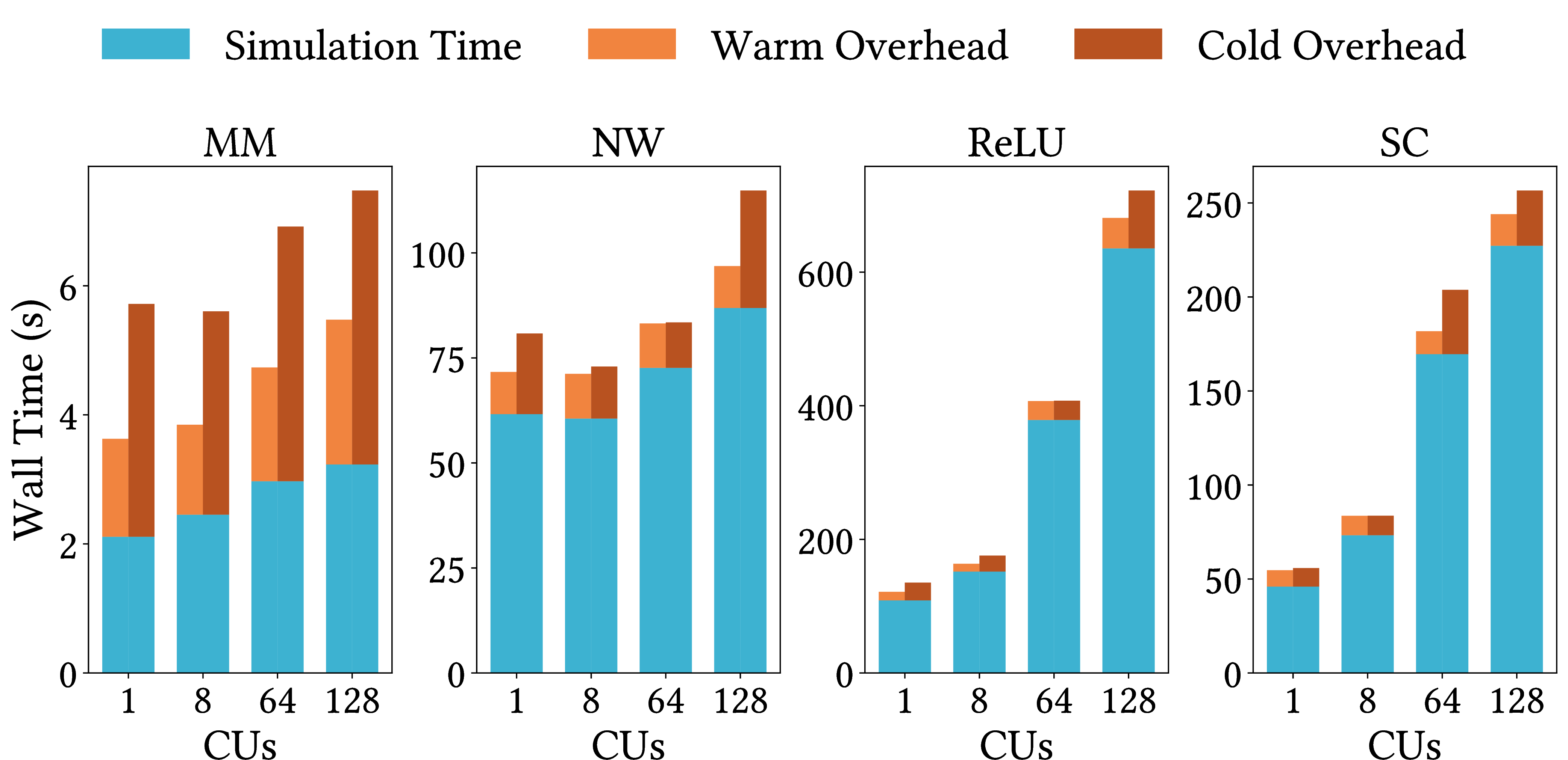
The true ArchSim overhead is 1.6 seconds per simulation. Configuration generation takes a median of 1.6 seconds (range 0.7–2.3s) across all configurations. All remaining overhead (warm: median 10.4s additional, cold: median 15.8s
additional) is go build compilation time, which any MGPUSim workflow pays when modifying and recompiling a configuration.
Overhead decreases with simulation length. For short simulations under 10 seconds (MM at 1–8 CUs, with 2.1–3.2s baseline), overhead reaches 64.3% because the 1.6s config generation and 10s compilation dominate a 2–3 second simulation. However, such short simulations are not representative of architectural studies. For medium simulations (10–100s, NW and SC at low CU counts), warm overhead is 15.5%. For realistic workloads of 100 seconds or more (ReLU and SC at 64–128 CUs), warm overhead falls to 8.1%, with the ArchSim-specific configuration generation cost accounting for just 0.25% of total wall time. Excluding MM, warm overhead is 11.8% mean (11.6% median) and cold overhead is 19.1% mean, with overhead consistently decreasing as simulation time grows.
The overhead ArchSim introduces is the price of eliminating 30 hand-written simulation programs, per-machine environment setup, orchestration scripts, and custom analysis pipelines for a \(5 \times 12\) study. For studies where simulation time dominates, which is the common case in architectural research, ArchSim’s overhead is negligible.
5 Case Study↩︎
We demonstrate ArchSim’s analysis capabilities through a case study that investigates the performance impact of cache hierarchy configurations across multiple benchmarks and compute-unit (CU) counts. The analysis is performed entirely through ArchSim’s interface, without writing any custom parsing or aggregation scripts.
Modern GPU architectures balance compute throughput against memory system complexity. Adding intermediate cache levels, such as a shared L1.5 between per-CU L1 caches and a global L2, or an L3 last-level cache below L2, can reduce traffic to main memory but introduces additional latency on the critical path. Understanding when deeper hierarchy helps versus hurts requires sweeping multiple configurations across workloads with different memory behaviors. Traditionally, each configuration requires modifying simulator source code and rebuilding; ArchSim reduces this to editing a declarative JSON configuration.
We define four architectural configurations by varying the cache hierarchy between the per-CU L1 caches and the ideal memory controller. The baseline routes requests through L1 \(\rightarrow\) L2 \(\rightarrow\) Memory Controller. The +L1.5 variant inserts a shared 4-way 64B-block L1.5 cache between L1 and L2. The +L3 variant appends a 16-way 128B-block L3 cache below L2. The Combined variant includes both, forming L1 \(\rightarrow\) L1.5 \(\rightarrow\) L2 \(\rightarrow\) L3 \(\rightarrow\) Memory Controller.
All four configurations use the same compute unit design, TLB hierarchy, and ideal memory controller. The only difference is the depth and structure of the data cache path. Each configuration is expressed as a self-contained ArchSim JSON file; no simulator code changes are required to move between them. Crucially, these configurations are not parameter variations over a fixed topology: the +L1.5 and +L3 variants differ in component presence (the L1.5 and L3 nodes are absent in the baseline), associativity (4-way vs.-way), block size (64B vs.128B), and structural wiring, each expressed as a declarative graph edit. This demonstrates that ArchSim’s configuration abstraction supports structural composition from the imported Models, not only parameter sweeps, across a space that spans component presence, integer-valued settings, and interconnect topology simultaneously.
We select three benchmarks that stress different parts of the memory system: ReLU, a streaming element-wise operation that is primarily memory-bandwidth bound; Matrix Multiply (MM), a compute-intensive kernel with high arithmetic density relative to memory traffic; and Matrix Transpose (MT), a stride-heavy access pattern that stresses cache line utilization and memory bandwidth. We run each configuration at three CU counts (1, 8, and 16) and at two problem-size tiers: a smaller tier suitable for local iteration and a larger tier representative of realistic workloads. The full experiment comprises 72 simulation runs, each launched from the same runner binary without modifying any simulator source code.
The current case study targets the MGPUSim/Akita ecosystem and three benchmark families. This reflects the scope of the current code generation backend rather than a limitation of the underlying experiment abstraction: the core concepts of configurations, experiment matrices, runners, and the artifact store are defined independently of any specific simulator, and extending the evaluation to additional simulators such as gem5 or SST is a priority for future work. Within the MGPUSim backend, the configuration interface additionally supports sweeping interconnect bandwidth, TLB size, memory controller count, and CU pipeline parameters, though a comprehensive evaluation across all these dimensions is left to future work.
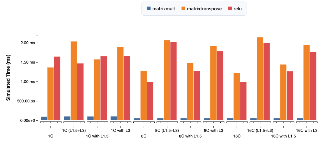
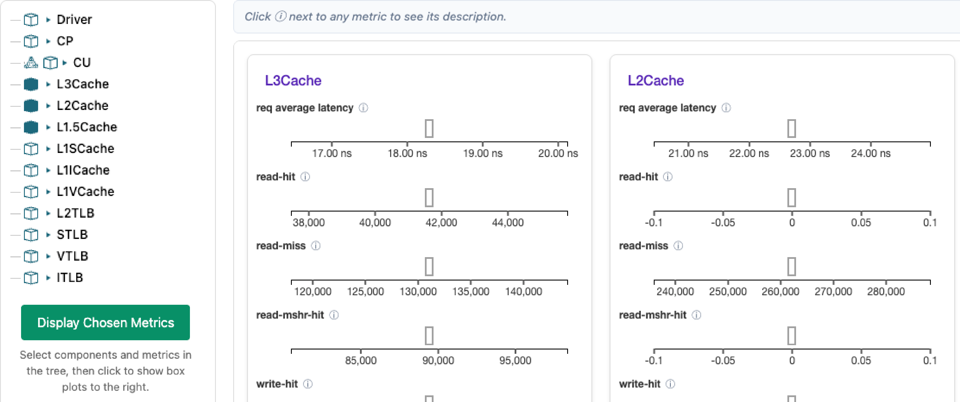
Figure 10: Case-study analysis views in ArchSim.. a — Experiment-level view for the cache hierarchy case study. Each group of bars corresponds to a (configuration, CU count) combination; bar height represents simulated execution time. The three benchmark series (matrixmult, matrixtranspose, relu) are shown in separate colors. The view enables direct identification of configurations where deeper cache hierarchies increase rather than decrease execution time., b — Component-level drill-down for the matrixtranspose benchmark on the 1C (L1.5+L3) configuration. The left panel shows the component hierarchy; the right panels show per-component metric timelines. The near-zero L2 read hit rates and nonzero L3 MSHR activity visible here explain the performance degradation identified in the experiment-level view.
Once the experiment completes, we navigate to the Analysis tab to explore the results. At the top of the tab, the experiment-level view (Figure 10 (a)) presents simulated execution time across all \((\textit{configuration}, \textit{benchmark})\) pairs, enabling direct comparison of performance trends across the entire experiment matrix.
Several insights can be immediately observed.
Workload sensitivity to memory hierarchy.
matrixmultexhibits consistently low execution time across all configurations. This is consistent with its compute-intensive nature and relatively small problem size (128\(\times\)128\(\times\)128), which limits its sensitivity to cache hierarchy changes. In contrast,matrixtransposeandrelushow substantial variation across configurations, suggesting stronger dependence on memory-system behavior due to their stride-heavy and streaming access patterns respectively.Deeper cache hierarchies do not universally improve performance. Configurations that include both L1.5 and L3 caches frequently exhibit higher execution time than simpler configurations. This indicates that additional cache levels may introduce overhead that outweighs their benefit for certain workloads.
Interaction between parallelism and memory hierarchy. Increasing CU count does not uniformly improve performance across all configurations. For configurations with deeper cache hierarchies such as Combined (L1.5+L3), performance at higher CU counts is sometimes higher than at lower CU counts, suggesting that the latency overhead of deeper hierarchies can outweigh the benefits of increased parallelism for certain workloads.
This view allows researchers to quickly identify anomalous or non-intuitive performance trends without constructing experiment-specific aggregation pipelines.
To explain the observed performance differences, we select a representative configuration: matrixtranspose on 1C (L1.5+L3). Selecting this point in the experiment-level view loads the component-level drill-down interface, which exposes hierarchical metrics for each hardware component. Figure 10 (b) shows an excerpt of this view, focusing on the L2 and L3 cache metrics most relevant to the observed performance degradation.
The drill-down reveals the following:
Ineffective intermediate cache level. The L2 cache exhibits near-zero read and write hit rates, indicating that it provides little filtering benefit for this workload. Most memory accesses pass through this level without reuse.
Useful deeper cache level. The L3 cache shows nonzero read-hit and MSHR-hit activity, indicating that some reuse is captured at this level.
Explaining performance degradation. The L2 cache adds 21–24 ns of average request latency while providing effectively zero hits, so every request pays this latency cost before reaching the L3. The combined overhead of traversing both levels without proportional reuse benefit explains the increased execution time observed in the experiment-level view.
This analysis demonstrates how ArchSim enables direct causal reasoning: from identifying a performance anomaly at the experiment level to diagnosing its architectural root cause at the component level.
6 Related Work↩︎
Widely used frameworks such as gem5 [2], Multi2Sim [5], [19], [20], GPGPU-Sim, Sniper [21], SST [4], and MGPUSim [7] provide detailed models for evaluating CPU and GPU architectures. These systems focus on modeling fidelity and execution performance; experiment structure remains implicit in the scripts and file organization that surround them. ArchSim builds on this ecosystem by introducing an experiment platform that represents simulation studies as structured entities and automatically generates the simulator programs required to execute them.
ReproZip [10] captures execution environments to support experiment replication. OCCAM [22] provides a software environment for creating reproducible research artifacts. MLflow [9] and Sacred [23] provide experiment tracking for machine learning workflows. Nextflow [24], Snakemake [25], and Kepler [26] support reproducible pipelines in data-intensive science. These systems target flat parameter spaces and scalar outputs and do not represent architecture simulation structure: hardware topology graphs, typed port bindings, and spatially organized component-level metrics. Within the architecture community, gem5art [27] captures configuration scripts, disk images, and simulator binary versions using Git-based artifact tracking. gem5art is the closest prior work to ArchSim’s version preservation design, but requires the researcher to explicitly tag each run with a version identifier and does not propagate version information to subsequent runs in the same experiment. ArchSim records simulator dependency versions automatically on the first successful run and reuses them for all subsequent runs without researcher intervention.
Daisen [13], Vis4Mesh [28], Ziabari et al. [29], and Ariel et al. [30] provide fine-grained visualization of GPU and accelerator execution behavior using simulation traces. gem5 also provides hierarchical statistics collection [2]. These tools analyze individual simulation runs; cross-run analysis requires custom parsing scripts. ArchSim operates at the experiment level, storing outputs as structured artifacts that support experiment-scoped metric retrieval and component-level exploration without intermediate parsing pipelines.
7 Conclusion↩︎
Computer architecture research increasingly relies on large-scale simulation studies that explore complex design spaces across many configurations and workloads. Yet the infrastructure supporting these studies evolves through collections of scripts, configuration programs, and analysis pipelines whose relationships remain implicit in code and directory structures, making studies fragile, difficult to reproduce, and hard to scale. ArchSim addresses this by treating simulation experiments as structured infrastructure objects: by making experiment structure explicit and machine-readable, the platform automates execution, artifact preservation, and analysis across the experiment lifecycle while preserving full compatibility with existing architecture simulators.
Looking forward, we envision simulation experiments becoming portable and shareable artifacts rather than collections of scripts tied to a particular environment. Such a shift would enable researchers to reuse architectural studies, reproduce prior results with minimal manual effort, and build shared infrastructure for exploring emerging architectural ideas. ArchSim represents one step toward this direction, and we believe that elevating experiment structure to a first-class concept can fundamentally improve how architecture simulation studies are created, executed, and shared.
We thank the National Science Foundation for its support under awards CNS-2234400 and CNS-2234401. Any opinions, findings, and conclusions or recommendations expressed in this material are those of the authors and do not necessarily reflect the views of the National Science Foundation.