ACID: Adaptive Caching for vIDeo generation
July 14, 2026
Abstract
Video diffusion models produce high-quality generations but remain slow at inference due to their sequential denoising procedure. Caching-based acceleration methods address this by reusing intermediate model outputs: leading dynamic approaches such as TeaCache, EasyCache, and DiCache accumulate a drift signal and skip expensive model evaluations when accumulated drift stays below a fixed threshold \(\tau\). This threshold controls an apparent tradeoff—raising it yields faster generation at the cost of visual quality, while lowering it preserves quality but sacrifices speed. We show this tradeoff is not fundamental; it is an artifact of holding \(\tau\) constant throughout denoising. We identify the existence of critical steps—timesteps where the drift signal changes rapidly—and show that applying a low threshold selectively at these steps while caching aggressively elsewhere recovers most of the quality of conservative caching at substantially higher inference speeds. Building on this insight, we propose ACID, a lightweight, training-free wrapper that monitors the rate of change of each method’s existing drift signal to dynamically switch between a low and a high threshold. ACID is signal-agnostic and modular: it requires no retraining and plugs directly into existing dynamic caching methods without modifying their core mechanisms. Evaluated across three caching methods (TeaCache, EasyCache, DiCache) and three open-source video diffusion models (HunyuanVideo, Wan 2.1, CogVideoX), ACID consistently expands the Pareto frontier of visual quality versus inference speed beyond what any fixed threshold achieves. In particular, on TeaCache and HunyuanVideo, ACID achieves up to \(2.16\times\) speedup over the no-caching baseline, and up to \(38\%\) additional speedup over the conservative fixed-threshold baseline with negligible (\(<0.3\) dB PSNR, \(<0.01\) SSIM, \(<0.01\) LPIPS) quality degradation.
1 Introduction↩︎
Video generation models [1]–[6] are becoming increasingly powerful in generating realistic videos [7]; however, their slow inference speed and high compute requirements (3 to 23 minutes for \({\sim}\)5-second videos on a single A100 GPU) pose an impediment to their wide adoption [8]. As these models scale to generate even higher resolutions, the challenges associated with slow inference speed and high computation requirements will be further exacerbated. The primary reason for these slow inference speeds and high computation needs is the core inference loop of these video generation models [1]–[6]: a computationally expensive diffusion backbone that runs a sequential denoising procedure, dominating generation time.
To alleviate this bottleneck, several approaches have been proposed [9]–[11]. These generation-accelerating approaches can be classified into two categories: training-based [10], [12]–[16] and training-free [9], [11], [17]–[19] acceleration strategies. Due to the significant overhead [11], [20], [21] associated with training-based approaches, which generally entail substantial compute, data, and cost, training-free acceleration methods have become particularly appealing. Among training-free methods, caching methods, due to their lightweight computation requirements, are being rapidly deployed. Caching methods leverage similarity between intermediate states and reuse them to reduce computational redundancy. Caching strategies have rapidly evolved from early uniform caching strategies that used fixed intervals to sophisticated methods [11], [20]–[23] which determine their caching strategy based on the similarity predicted at each step, thus adapting caching to the behavior of the diffusion process.
All of the dynamic caching strategies—such as TeaCache [11], EasyCache [21], and DiCache [20]—share a common structure: they use an accumulated drift metric that estimates the change in model output. If this accumulated drift is below a user-provided threshold, they skip the expensive model run and reuse the previous output with some correction. If the accumulated drift exceeds the threshold, they run the full model and reset the accumulated drift to zero.
Choosing this threshold presents a seemingly inherent tradeoff between output quality and inference latency. A high threshold caches more aggressively, yielding faster generation but lower quality. A low threshold caches conservatively, preserving quality but sacrificing speed.
This raises a fundamental question: is this tradeoff between output quality and inference latency actually fundamental? In this work, we show that it is not. It is instead an artifact of using a fixed threshold throughout the sequential denoising procedure. When the threshold is chosen adaptively, the quality-latency tradeoff can be improved relative to any fixed-threshold dynamic caching method. Figure 1 shows that a dynamic threshold method can push the Pareto frontier beyond that of any fixed-threshold method.
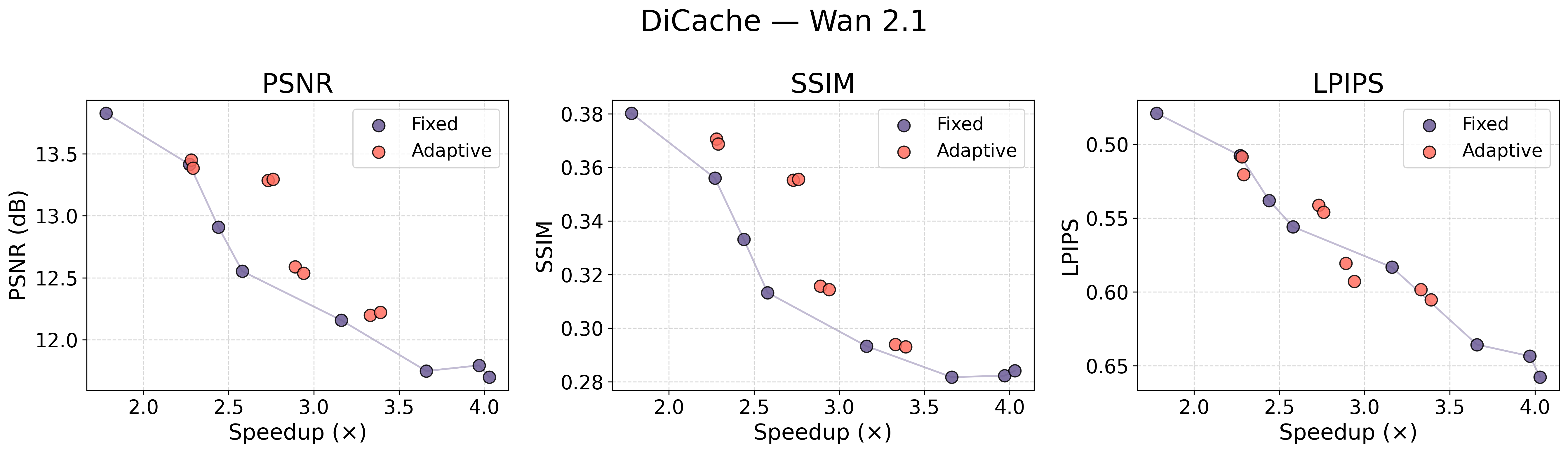
We attribute the power of adaptive threshold schemes to the existence of critical steps in the sequential denoising procedure. By avoiding aggressive caching during these critical steps, our method mitigates the quality loss that fixed-threshold dynamic caching methods typically exhibit. This means one can design an adaptive scheme that identifies critical steps and adjusts the threshold accordingly. Based on these findings, we propose ACID, a simple but powerful adaptive threshold caching mechanism that generalizes across different dynamic caching methods and models, while imposing low computational overhead. ACID examines the rate of change of the respective method’s metric to detect critical steps and adjust thresholds dynamically, improving performance without sacrificing output quality.
Our experiments show that ACID achieves reduced inference latency while maintaining output quality on video generation tasks. In particular, on TeaCache and HunyuanVideo, ACID achieves up to \(2.16\times\) speedup over the no-caching baseline, and up to \(38\%\) additional speedup over the conservative fixed-threshold baseline with negligible (\(<0.3\) dB PSNR, \(<0.01\) SSIM, \(<0.01\) LPIPS) quality degradation.
We summarize our contributions below:
We identify the existence of critical steps in the sequential denoising procedure and show that video generation caching methods must account for them.
We design ACID, an adaptive threshold dynamic caching mechanism that switches between low and high thresholds based on the second derivative of each method’s metric. This signals critical steps in the denoising process, enabling significant performance improvements without sacrificing output quality.
We provide empirical evaluation across several dynamic caching methods (TeaCache, EasyCache, DiCache) and several diffusion models (HunyuanVideo, Wan 2.1, CogVideoX).
2 Related Work↩︎
2.0.0.1 Diffusion Models.
While U-Net-based diffusion models like Stable Diffusion [24] and SDXL [25] successfully catalyzed high-quality image and video generation [26]–[28], their limited architectural capacity bottlenecks the training and deployment of massive models. To eliminate this constraint, recent frameworks have rapidly shifted toward the Diffusion Transformer (DiT) backbone, exploiting its structural flexibility to support next-generation foundation models [29]–[32]. However, despite their theoretical promise, scaling these DiT backbones introduces substantial computational overhead.
2.0.0.2 Diffusion Model Acceleration.
As DiT backbones scale in capacity and complexity, their runtime increases proportionately, exacerbating the notoriously slow inference speeds of diffusion models and impeding real-world deployment. To alleviate this latency bottleneck, several acceleration paradigms have emerged. Recent work has extensively explored efficient attention [10], [33], sparse attention [18], [19], distillation [12]–[14], quantization [10], and improved SDE/ODE solvers [9]. Alongside these methods, caching-based feature reuse strategies offer a particularly compelling, orthogonal path forward, which we detail next.
2.0.0.3 Caching-based feature reuse strategies.
Caching methods have gained attention recently due to their lightweight nature. DeepCache [34] and Faster Diffusion [35] reuse U-Net features across timesteps to reduce computational redundancy. FORA [36] and \(\Delta\)-DiT [37] extend this idea to transformer-based architectures. PAB [38] broadcasts attention features to later timesteps in a pyramid-style method based on various block characteristics. AdaCache [22] modifies residual reuse methods based on content complexity. FasterCache [39] proposes to cache for both the conditional and unconditional branch of Classifier Free Guidance [40]. TeaCache [11], EasyCache [21], and DiCache [20] represent the most recent state-of-the-art dynamic caching approaches; we examine their shared structure and its key limitation in the paragraphs below.
2.0.0.4 The Fixed Threshold of Dynamic Feature Caching Methods.
Many recent dynamic caching-based feature reuse strategies make caching decisions based on the diffusion process’s state at runtime. Methods like TeaCache, EasyCache, and DiCache share a common algorithmic skeleton: a running accumulated drift variable is initialized to zero, an estimate of output change is added at each step, and this accumulated value is compared against a fixed threshold \(\tau\). When the accumulated drift is below \(\tau\), the expensive model forward pass is skipped and the previous output is reused with some correction. When the accumulated drift exceeds \(\tau\), the full model is run and the accumulator is reset. The methods differ in how they estimate drift and how they reconstruct the output on skipped steps, which we delve into below.
2.0.0.5 TeaCache.
TeaCache estimates drift using the L1 distance between consecutive values of the Timestep Embedding Modulated Noisy Input (TEMNI), a combination of the text embedding, timestep embedding, and current noisy input. Rather than measuring how much the model output changed, which would require running the model, TeaCache measures how much the model’s inputs changed, exploiting the empirical observation that large input changes correlate with large output changes. On skipped steps, TeaCache reuses the previous output with a stored residual correction.
2.0.0.6 EasyCache.
EasyCache estimates drift using the model’s transformation rate \(k\), defined as the ratio of output change to input change at the most recently computed step. The authors observe that \(k\) is unstable early in the denoising process but quickly stabilizes, reflecting the model settling into a roughly linear input-output regime. Under this regime, EasyCache estimates the current step’s output change as \(k \times \Delta\text{input} / \|v_{t-1}\|\), where \(\Delta\text{input}\) is the current input change, \(\|v_{t-1}\|\) is the magnitude of the previous output, and \(k\) is the transformation rate of the last fully computed step. This normalized estimate is accumulated against \(\tau\). On skipped steps, EasyCache reconstructs the output as the current input plus the offset \(\Delta = \text{output} - \text{input}\) from the last fully computed step, which is justified because a stable \(k\) implies the model’s additive contribution is approximately constant.
2.0.0.7 DiCache.
DiCache replaces the input-level proxy used by TeaCache and EasyCache with a feature-level proxy. At each step, DiCache runs only the first few transformer blocks of the model as a shallow probe and measures how much those features changed. Because these early layers are cheap to compute, this provides a direct estimate of whether the full model’s output would change significantly, without paying the cost of a full forward pass. On skipped steps, DiCache uses the trajectory of shallow probe features across multiple recent steps to interpolate a better estimate of the current deep output.
Despite these differences, all three methods share a critical limitation: the fixed user-provided threshold is held constant throughout the entire denoising process. This means the caching schedule cannot respond to the diffusion process’s varying dynamics. Our work identifies this fixed threshold as the source of the quality-latency tradeoff observed in prior methods, and proposes an adaptive and modular threshold mechanism on top of methods like TeaCache, EasyCache, and DiCache that modulates \(\tau\) based on the local rate of change of each method’s metric, enabling more aggressive caching in stable regions and more conservative caching at critical steps.
3 ACID↩︎
In this section, we introduce ACID, a method for adaptively varying caching frequency.
3.1 Preliminaries↩︎
3.1.0.1 Denoising Diffusion Models.
At inference time, diffusion models generate content through several sequential denoising steps. The core idea is to start with random noise and iteratively refine it until it approximates a sample from the target distribution. During training (the forward diffusion process), Gaussian noise is incrementally added over \(T\) steps to a sample datapoint \(x_0\) from a data distribution: \[x_t = \sqrt{\alpha_t} \, x_{t-1} + \sqrt{1 - \alpha_t} \, z_t, \quad t = 1, \ldots, T\] where \(\alpha_t \in [0, 1]\) governs the noise level and \(z_t \sim \mathcal{N}(0, I)\) represents Gaussian noise. As \(t\) increases, \(x_t\) becomes progressively noisier, ultimately approaching a standard normal distribution at \(t = T\). The reverse diffusion process, which is what we perform at inference time, is designed to reconstruct the original sample from the noise: \[p_\theta(x_{t-1} \mid x_t) = \mathcal{N}\!\left(x_{t-1};\, \mu_\theta(x_t, t),\, \Sigma_\theta(x_t, t)\right)\] where \(\mu_\theta\) and \(\Sigma_\theta\) are learned parameters defining the mean and covariance.
3.2 Analysis↩︎
3.2.0.1 Analyzing Caching Metrics.
To understand the limitations of fixed-threshold caching, we analyze how caching signals evolve throughout the denoising process. We begin with TeaCache’s \(\Delta\)TEMNI as a representative signal, since TeaCache is one of the earliest dynamic caching methods for video diffusion models and thus a natural starting point for analysis. We find that these structural properties generalize across other caching signals, motivating the general adaptive framework we propose.
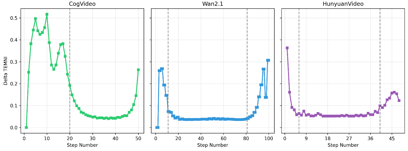
Preliminary analysis of the \(\Delta\)TEMNI metric from TeaCache reveals two empirical properties of caching signals. First, these metrics remain relatively consistent across diverse prompts, as illustrated in Figure 2. Second, the structural behavior of these signals is model-dependent, as shown in Figure 3; specifically, HunyuanVideo and Wan 2.1 exhibit a characteristic U-shaped pattern, whereas CogVideoX demonstrates a distinctly different distribution. Based on these observations, we evaluate our proposed solution across three models (HunyuanVideo, Wan 2.1, and CogVideoX), which together cover both signal pattern types and ensure robustness against their varying behaviors.
As Figures 2 and 3 show, there are certain parts of the diffusion process where \(\Delta\)output and \(\Delta\)TEMNI are relatively high, and other parts where \(\Delta\)TEMNI is low. Dynamic feature caching methods already take this into account: when the predicted \(\Delta\)output is greater, they cache less often (because they hit the fixed threshold more often), and when the predicted \(\Delta\)output is smaller, they cache more often (they hit the fixed threshold less often). But while dynamic caching methods do find a better speed–quality tradeoff than the no-caching baseline, we find that this tradeoff is not optimal: the degree to which they cache more in stable zones or cache less in unstable zones is suboptimal—a limitation imposed by the single fixed threshold. We find that using different thresholds for different parts of the diffusion process—such as low thresholds for unstable regions and high thresholds for stable regions—leads to a better speed–quality tradeoff.
We could attribute the gains from adaptive thresholding to a suboptimal metric for TeaCache, but we importantly find the same gains from adaptive thresholding for EasyCache and DiCache as well, which use entirely different caching signals. This suggests the limitation is structural: any method that applies a single fixed threshold throughout the denoising process will face this suboptimality, regardless of the signal it uses.


To find a method with a better speed–quality tradeoff than any fixed-threshold approach, we ran a small experiment. Using TeaCache on HunyuanVideo, we compared a low fixed threshold, a high fixed threshold, and a range of two-threshold configurations in which we varied the transition point between the low and high threshold. We repeated this across two additional open-source models: Wan 2.1 and CogVideoX. Figure 4 shows the \(\Delta\)TEMNI signal throughout the denoising process for each model, with dashed lines marking the transition points at which a dual-threshold configuration had a better speed–quality tradeoff than both fixed-threshold baselines.
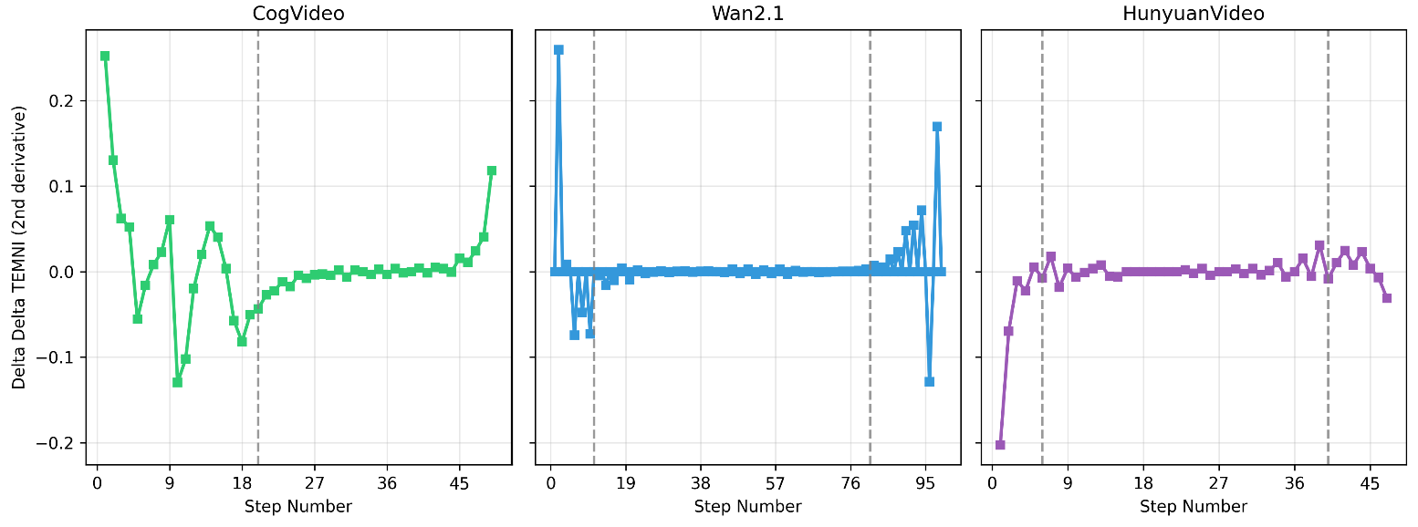
We then asked: what signal determines where these optimal transition points fall? Examining the second derivative of the TEMNI signal (Figure 5), we found that the optimal transition points coincide with the step at which the second derivative stabilizes—transitioning from a variable regime to a stable one. This suggests that the rate of change of the caching signal is a natural indicator of when to switch thresholds.
3.3 Adaptive Threshold Caching↩︎
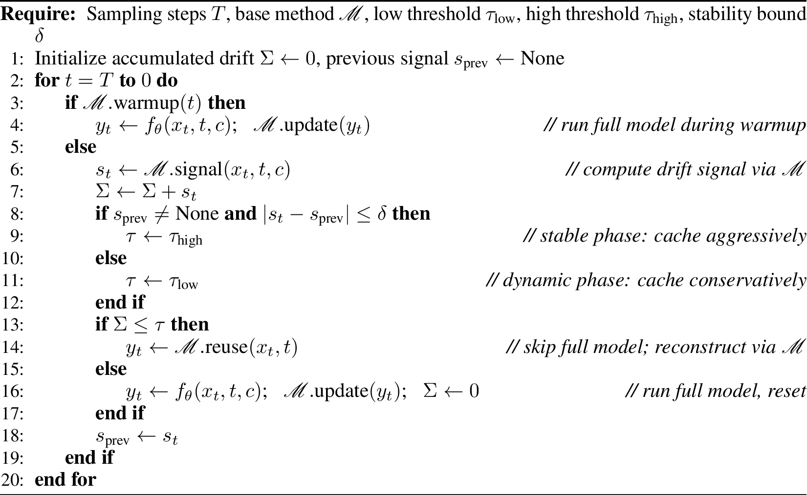
ACID extends the single-threshold framework of methods like TeaCache, EasyCache, and DiCache with a dual-threshold strategy. Rather than applying a single fixed threshold \(\tau\), we maintain two thresholds: a high threshold \(\tau_{\text{high}}\) and a low threshold \(\tau_{\text{low}}\). The active threshold is selected based on the rate of change of the underlying signal of the dynamic caching method (\(\Delta\)TEMNI for TeaCache, \(k \times \Delta\text{input} / \|v_{t-1}\|\) for EasyCache, and \(\Delta\)probe features for DiCache).
When the rate of change is within [\(-\delta\), \(\delta\)], indicating a stable phase of the diffusion process, we apply \(\tau_{\text{high}}\), permitting more aggressive caching. When the rate of change escapes this [\(-\delta\), \(\delta\)] safe zone, indicating a more dynamic and quality-critical phase, we apply \(\tau_{\text{low}}\), restricting caching to preserve output fidelity.
This reflects the key observation that certain parts of the diffusion process are more important to preserve than others, and that the diffusion process cannot be treated as uniform throughout.
4 Experiments↩︎
4.1 Experimental Setup↩︎
4.1.0.1 Base models.
We evaluate on three open-source video generation diffusion models: HunyuanVideo T2V 720P [6], Wan 2.1 T2V 1.3B [4], and CogVideoX 1.5-5B [41].
4.1.0.2 Compared methods.
We apply our adaptive threshold framework on top of three base caching methods: TeaCache (evaluated on HunyuanVideo, Wan 2.1, CogVideoX), EasyCache (evaluated on HunyuanVideo, Wan 2.1), and DiCache (evaluated on HunyuanVideo, Wan 2.1). EasyCache and DiCache are not evaluated on CogVideoX because neither method provides an official implementation for that model; we restrict our evaluation to officially supported configurations to avoid confounding results from self-implemented ports. For each method–model combination, we compare a no-caching baseline, the fixed-threshold method with several threshold values spanning a low-to-high range, and our adaptive dual-threshold variant ACID with several low/high threshold values.
4.1.0.3 Evaluation metrics.
Following TeaCache, we evaluate along two dimensions: inference efficiency and visual quality. For inference efficiency, we report inference latency and speedup, defined as the ratio of the no-caching baseline latency to the method latency for the same model. For visual quality, we use LPIPS, PSNR, and SSIM, computed by comparing cached-method outputs against the no-caching baseline.
4.1.0.4 Implementation details.
All experiments were carried out on NVIDIA A100 80GB PCIe GPUs with PyTorch. We selected 33 prompts from VBench’s [42] prompt set: 3 prompts per group across 11 groups, where each group corresponds to one or more VBench evaluation dimensions, together spanning all 16 VBench dimensions. For each method–model combination, we generated 33 videos per configuration (one per prompt) across all evaluated threshold settings, using a fixed seed throughout.
4.2 Main Results↩︎
| Method | Model | Mode | Latency | Speedup | PSNR \(\uparrow\) | SSIM \(\uparrow\) | LPIPS \(\downarrow\) |
|---|---|---|---|---|---|---|---|
| TeaCache | HunyuanVideo | Baseline | 1359s | 1.00\(\times\) | — | — | — |
| Fixed (lo, 0.1) | 864s | 1.57\(\times\) | 24.69 | 0.819 | 0.187 | ||
| Fixed (hi, 0.3) | 424s | 3.20\(\times\) | 19.98 | 0.693 | 0.353 | ||
| Adaptive | 628s | 2.16\(\times\) | 24.41 | 0.813 | 0.196 | ||
| Wan 2.1 | Baseline | 212s | 1.00\(\times\) | — | — | — | |
| Fixed (lo, 0.05) | 150s | 1.42\(\times\) | 24.93 | 0.845 | 0.083 | ||
| Fixed (hi, 0.2) | 74s | 2.86\(\times\) | 17.10 | 0.538 | 0.335 | ||
| Adaptive | 108s | 1.96\(\times\) | 22.10 | 0.757 | 0.150 | ||
| CogVideoX 1.5 | Baseline | 1019s | 1.00\(\times\) | — | — | — | |
| Fixed (lo, 0.1) | 723s | 1.41\(\times\) | 37.32 | 0.958 | 0.029 | ||
| Fixed (hi, 0.3) | 465s | 2.19\(\times\) | 16.35 | 0.580 | 0.463 | ||
| Adaptive | 545s | 1.87\(\times\) | 32.02 | 0.930 | 0.058 | ||
| EasyCache | HunyuanVideo | Baseline | 1357s | 1.00\(\times\) | — | — | — |
| Fixed (lo, 0.025) | 659s | 2.06\(\times\) | 33.51 | 0.926 | 0.058 | ||
| Fixed (hi, 0.045) | 531s | 2.55\(\times\) | 28.99 | 0.851 | 0.153 | ||
| Adaptive | 568s | 2.39\(\times\) | 30.62 | 0.894 | 0.094 | ||
| Wan 2.1 | Baseline | 216s | 1.00\(\times\) | — | — | — | |
| Fixed (lo, 0.020) | 125s | 1.73\(\times\) | 25.58 | 0.852 | 0.087 | ||
| Fixed (hi, 0.040) | 102s | 2.12\(\times\) | 22.02 | 0.750 | 0.148 | ||
| Adaptive | 113s | 1.92\(\times\) | 24.90 | 0.833 | 0.100 | ||
| DiCache | HunyuanVideo | Baseline | 1265s | 1.00\(\times\) | — | — | — |
| Fixed (lo, 0.05) | 659s | 1.92\(\times\) | 30.96 | 0.904 | 0.088 | ||
| Fixed (hi, 0.10) | 419s | 3.02\(\times\) | 20.15 | 0.720 | 0.328 | ||
| Adaptive | 620s | 2.04\(\times\) | 29.42 | 0.888 | 0.105 | ||
| Wan 2.1 | Baseline | 224s | 1.00\(\times\) | — | — | — | |
| Fixed (lo, 0.07) | 99s | 2.27\(\times\) | 13.41 | 0.356 | 0.508 | ||
| Fixed (hi, 0.225) | 56s | 3.97\(\times\) | 11.79 | 0.282 | 0.644 | ||
| Adaptive | 82s | 2.73\(\times\) | 13.29 | 0.355 | 0.541 |
The Pareto plots in Appendix 6 show the efficiency and visual quality tradeoff offered by fixed-threshold methods, and how our adaptive dual-threshold method consistently expands the fixed-threshold Pareto frontier for each of the seven caching method and diffusion model combinations.
Table 1 shows the efficiency and visual quality of notable adaptive mode points for each feature caching method and diffusion model combination, comparing them to the baseline mode, the fixed-threshold mode using the low threshold of the adaptive mode, and the fixed-threshold mode using the high threshold of the adaptive mode.
4.2.0.1 TeaCache.
For TeaCache and HunyuanVideo, the adaptive mode achieves a 2.16\(\times\) speedup, between the low-threshold fixed mode’s speedup of 1.57\(\times\) and the high-threshold fixed mode’s speedup of 3.20\(\times\), while offering fidelity scores very similar to those of the low-threshold mode.
For TeaCache and Wan 2.1, the adaptive mode achieves a speedup of 1.96\(\times\), between the low-threshold fixed mode’s speedup of 1.42\(\times\) and the high-threshold fixed mode’s speedup of 2.86\(\times\), while retaining quality far closer to the low-threshold mode than to the high-threshold mode.
For TeaCache and CogVideoX, the adaptive mode achieves a speedup of 1.87\(\times\), between the low-threshold fixed mode’s speedup of 1.41\(\times\) and the high-threshold fixed mode’s speedup of 2.19\(\times\), again retaining quality far closer to the low-threshold mode than to the high-threshold mode.
Figure 7 shows how ACID’s adaptive modes surpass the Pareto frontier curves for all three diffusion models when used with TeaCache.
4.2.0.2 EasyCache.
For EasyCache and HunyuanVideo, our adaptive mode achieves a speedup of 2.39\(\times\), much closer to the high-threshold fixed mode’s speedup of 2.55\(\times\) than to the low-threshold fixed mode’s speedup of 2.06\(\times\), with quality metrics falling between those of the two fixed modes.
For EasyCache and Wan 2.1, our adaptive mode achieves a speedup of 1.92\(\times\), falling between the low- and high-threshold fixed mode speedups of 1.73\(\times\) and 2.12\(\times\), while retaining quality far closer to the low-threshold mode than to the high-threshold mode.
Figure 8 shows how several of ACID’s adaptive threshold modes surpass the Pareto frontier curves for both diffusion models when used with EasyCache.
We also note that EasyCache, by running the full model for the first few diffusion steps, already supports our main idea: varying the threshold across the diffusion process—in this case using a threshold of 0 (full computation) at the beginning and a higher threshold later—leads to a better quality–efficiency tradeoff.
4.2.0.3 DiCache.
For DiCache and HunyuanVideo, the adaptive mode achieves a speedup of 2.04\(\times\), falling between the low- and high-threshold speedups of 1.92\(\times\) and 3.02\(\times\), while achieving visual quality very close to the low-threshold mode and much better than the high-threshold mode.
For DiCache and Wan 2.1, the adaptive mode achieves a speedup of 2.73\(\times\), falling between the low- and high-threshold speedups of 2.27\(\times\) and 3.97\(\times\), while achieving visual quality very close to the low-threshold mode and much better than the high-threshold mode.
Figure 9 in Appendix 6 shows how several of ACID’s adaptive modes surpass the Pareto frontier curve for both diffusion models when used with DiCache.
5 Conclusion↩︎
We proposed ACID, a dynamic dual-threshold caching method for accelerating video diffusion model inference. By applying a high caching threshold during stable phases of the diffusion process and a low threshold during quality-critical phases, identified via the rate of change of each method’s caching signal, our method improves the Pareto frontier in the video quality vs.generation speed space over any fixed-threshold dynamic caching method. Experiments across three open-source video generation models and three caching methods confirm that ACID achieves near-low-threshold visual quality with substantially higher inference speedup.
6 Pareto Frontier Plots↩︎
Figures 7–9 show Pareto frontier plots for all evaluated method–model combinations. Each plot compares fixed-threshold configurations across a range of thresholds against our adaptive dual-threshold variants. In each case, adaptive points expand the frontier beyond what any fixed threshold achieves.
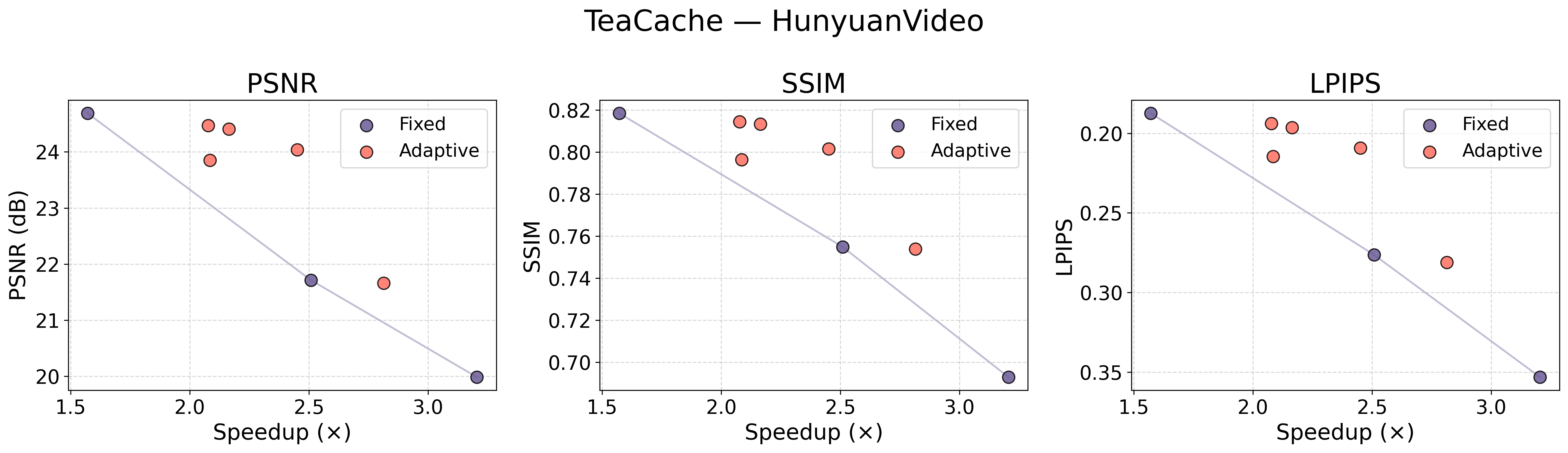
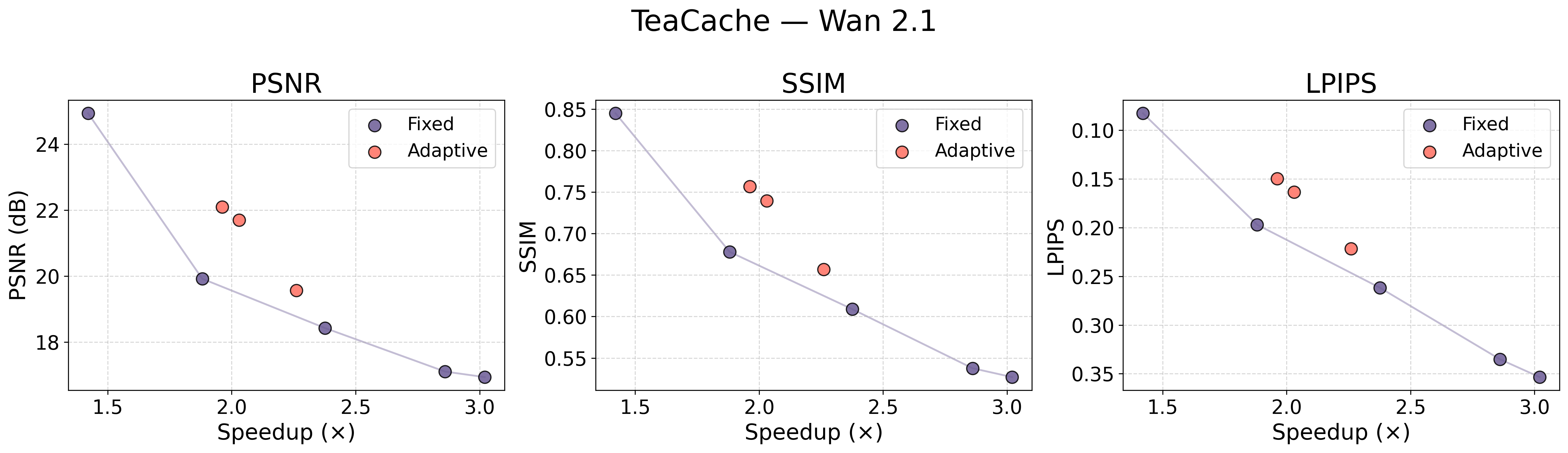
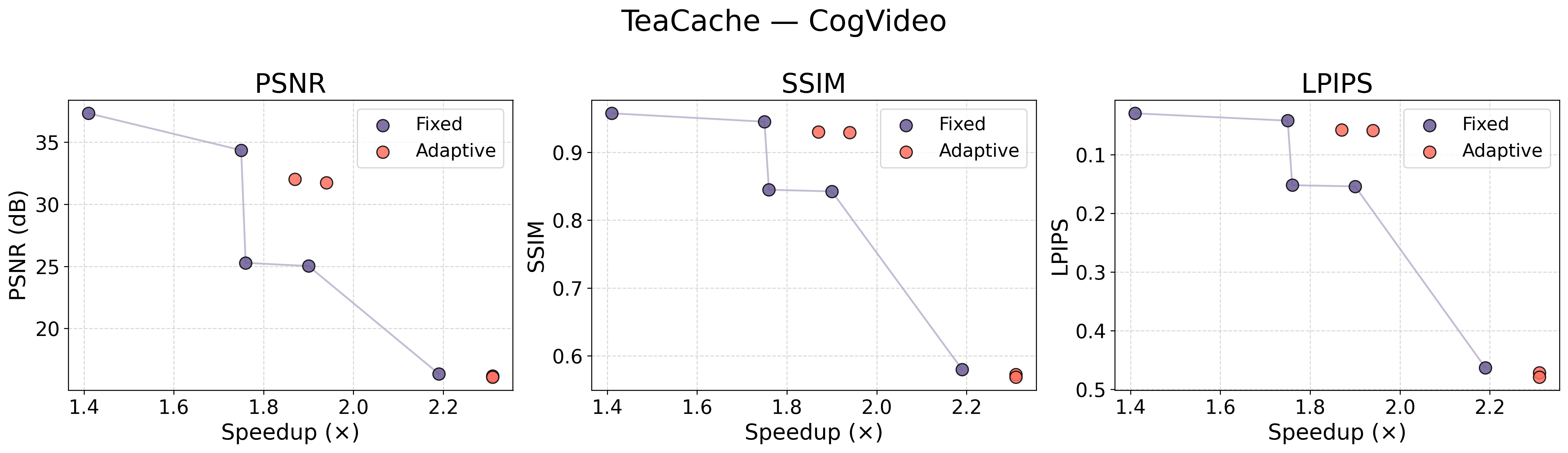
Figure 7: TeaCache Pareto frontiers across all three models. Adaptive modes (colored markers) expand the frontier beyond any fixed-threshold configuration (gray markers).. a — HunyuanVideo, b — Wan 2.1, c — CogVideoX 1.5
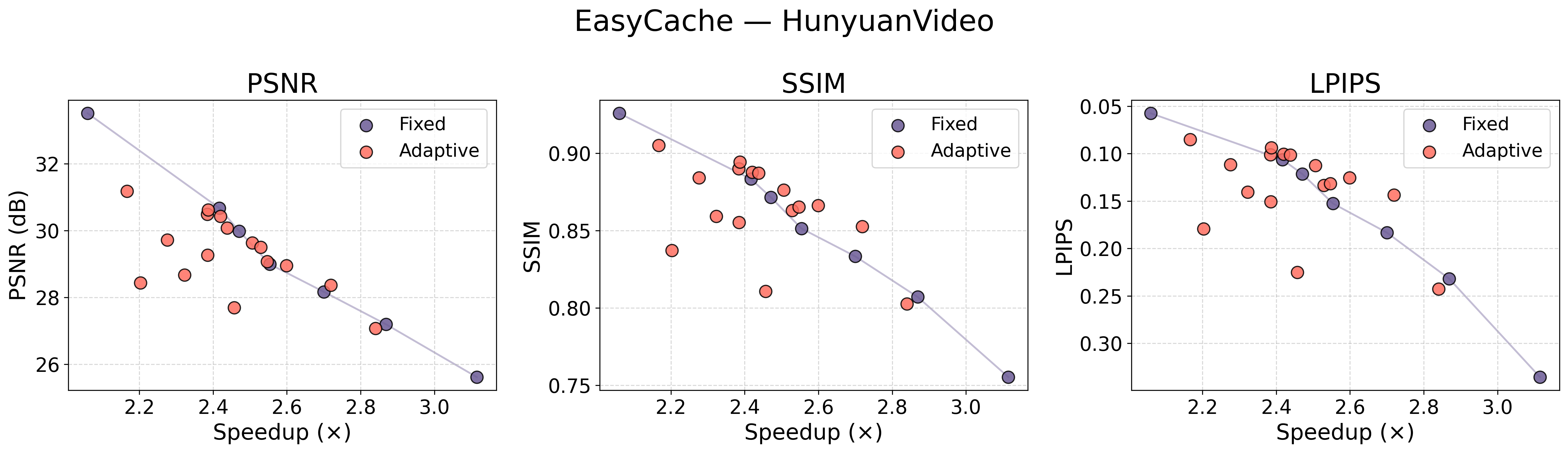
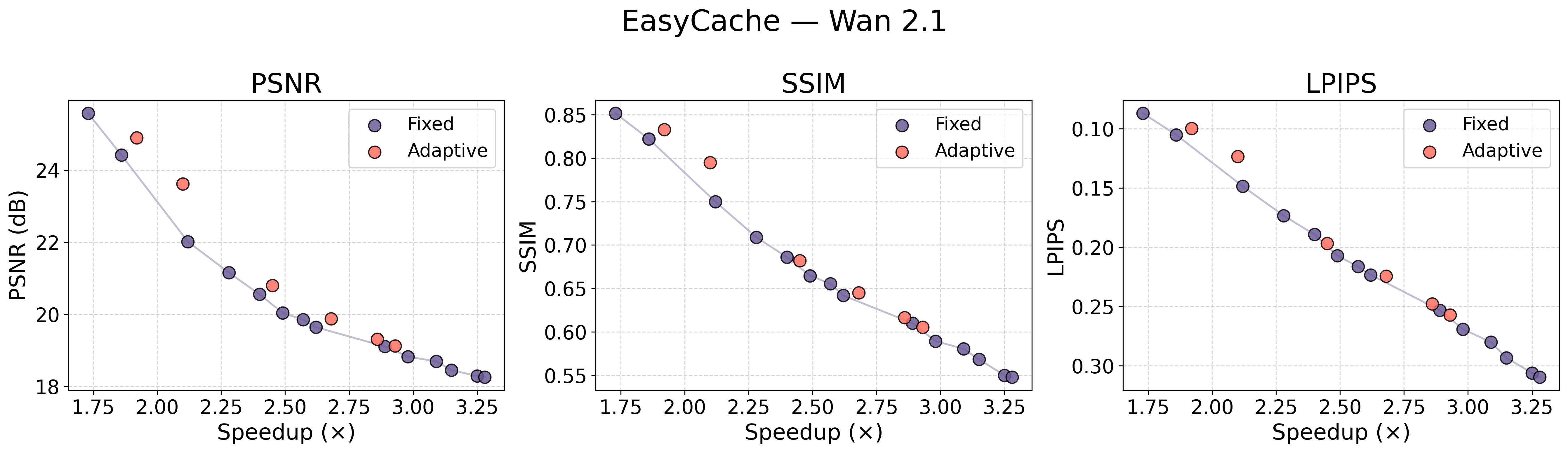
Figure 8: EasyCache Pareto frontiers. Adaptive modes expand the frontier beyond any fixed-threshold configuration.. a — HunyuanVideo, b — Wan 2.1
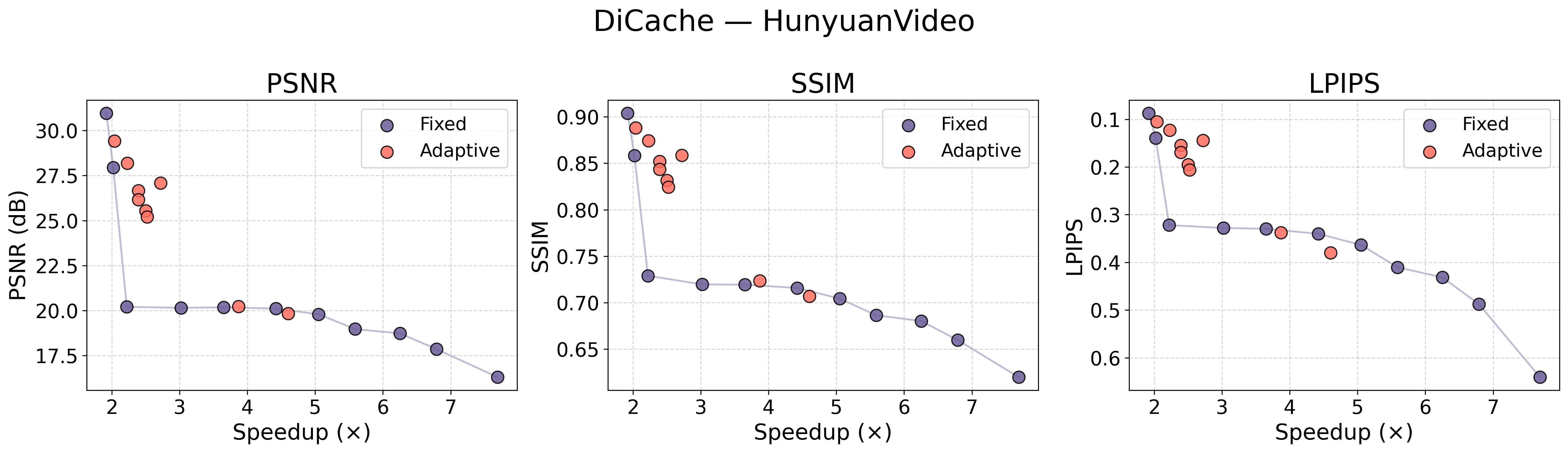
Figure 9: DiCache Pareto frontiers. Adaptive modes expand the frontier beyond any fixed-threshold configuration.. a — HunyuanVideo, b — Wan 2.1
7 Detailed Per-Combo Results↩︎
All configurations evaluated for each method \(\times\) model combination are listed below, sorted by increasing speedup. Bold rows are adaptive modes. Fidelity metrics (PSNR, SSIM, LPIPS) are computed against the uncached baseline. \(\tau\) denotes the caching threshold for all methods (cache-reuse residual for TeaCache/EasyCache; feature-difference score for DiCache). Subscripts \(\ell\)/\(h\) mark the low/high threshold in adaptive modes. Adaptive rows that share the same threshold pair differ in the stability bound \(\delta\).
| Mode | Latency | Speedup | PSNR \(\uparrow\) | SSIM \(\uparrow\) | LPIPS \(\downarrow\) |
|---|---|---|---|---|---|
| Fixed (\(\tau=0.1\)) | 864s | 1.57\(\times\) | 24.69 | 0.819 | 0.187 |
| Adaptive (\(\tau_\ell=0.1\), \(\tau_h=0.25\)) | 654s | 2.08\(\times\) | 24.47 | 0.814 | 0.194 |
| Adaptive (\(\tau_\ell=0.1\), \(\tau_h=0.2\)) | 652s | 2.09\(\times\) | 23.85 | 0.796 | 0.215 |
| Adaptive (\(\tau_\ell=0.1\), \(\tau_h=0.3\)) | 628s | 2.16\(\times\) | 24.41 | 0.813 | 0.196 |
| Adaptive (\(\tau_\ell=0.15\), \(\tau_h=0.3\)) | 554s | 2.45\(\times\) | 24.04 | 0.802 | 0.209 |
| Fixed (\(\tau=0.2\)) | 542s | 2.51\(\times\) | 21.71 | 0.755 | 0.276 |
| Adaptive (\(\tau_\ell=0.2\), \(\tau_h=0.3\)) | 483s | 2.81\(\times\) | 21.66 | 0.754 | 0.281 |
| Fixed (\(\tau=0.3\)) | 424s | 3.20\(\times\) | 19.98 | 0.693 | 0.353 |
5pt
| Mode | Latency | Speedup | PSNR \(\uparrow\) | SSIM \(\uparrow\) | LPIPS \(\downarrow\) |
|---|---|---|---|---|---|
| Fixed (\(\tau=0.05\)) | 150s | 1.42\(\times\) | 24.93 | 0.845 | 0.083 |
| Fixed (\(\tau=0.1\)) | 113s | 1.88\(\times\) | 19.92 | 0.678 | 0.197 |
| Adaptive (\(\tau_\ell=0.05\), \(\tau_h=0.2\)) | 108s | 1.96\(\times\) | 22.10 | 0.757 | 0.150 |
| Adaptive (\(\tau_\ell=0.05\), \(\tau_h=0.25\)) | 105s | 2.03\(\times\) | 21.69 | 0.739 | 0.164 |
| Adaptive (\(\tau_\ell=0.1\), \(\tau_h=0.2\)) | 94s | 2.26\(\times\) | 19.56 | 0.657 | 0.222 |
| Fixed (\(\tau=0.15\)) | 89s | 2.38\(\times\) | 18.42 | 0.609 | 0.262 |
| Fixed (\(\tau=0.2\)) | 74s | 2.86\(\times\) | 17.10 | 0.538 | 0.335 |
| Fixed (\(\tau=0.25\)) | 70s | 3.02\(\times\) | 16.94 | 0.527 | 0.354 |
5pt
| Mode | Latency | Speedup | PSNR \(\uparrow\) | SSIM \(\uparrow\) | LPIPS \(\downarrow\) |
|---|---|---|---|---|---|
| Fixed (\(\tau=0.1\)) | 723s | 1.41\(\times\) | 37.32 | 0.958 | 0.029 |
| Fixed (\(\tau=0.2\)) | 582s | 1.75\(\times\) | 34.35 | 0.945 | 0.042 |
| Fixed (\(\tau=0.22\)) | 579s | 1.76\(\times\) | 25.28 | 0.845 | 0.152 |
| Adaptive (\(\tau_\ell=0.1\), \(\tau_h=0.3\)) | 545s | 1.87\(\times\) | 32.02 | 0.930 | 0.058 |
| Fixed (\(\tau=0.25\)) | 536s | 1.90\(\times\) | 25.03 | 0.843 | 0.154 |
| Adaptive (\(\tau_\ell=0.1\), \(\tau_h=0.3\)) | 525s | 1.94\(\times\) | 31.74 | 0.929 | 0.059 |
| Fixed (\(\tau=0.3\)) | 465s | 2.19\(\times\) | 16.35 | 0.580 | 0.463 |
| Adaptive (\(\tau_\ell=0.30\), \(\tau_h=0.35\)) | 441s | 2.31\(\times\) | 16.18 | 0.572 | 0.472 |
| Adaptive (\(\tau_\ell=0.30\), \(\tau_h=0.40\)) | 441s | 2.31\(\times\) | 16.08 | 0.568 | 0.479 |
5pt
| Mode | Latency | Speedup | PSNR \(\uparrow\) | SSIM \(\uparrow\) | LPIPS \(\downarrow\) |
|---|---|---|---|---|---|
| Fixed (\(\tau=0.025\)) | 659s | 2.06\(\times\) | 33.51 | 0.926 | 0.058 |
| Adaptive (\(\tau_\ell=0.010\), \(\tau_h=0.050\)) | 626s | 2.17\(\times\) | 31.18 | 0.905 | 0.085 |
| Adaptive (\(\tau_\ell=0.010\), \(\tau_h=0.120\)) | 616s | 2.20\(\times\) | 28.43 | 0.837 | 0.179 |
| Adaptive (\(\tau_\ell=0.010\), \(\tau_h=0.075\)) | 596s | 2.28\(\times\) | 29.72 | 0.884 | 0.112 |
| Adaptive (\(\tau_\ell=0.010\), \(\tau_h=0.100\)) | 584s | 2.32\(\times\) | 28.67 | 0.859 | 0.141 |
| Adaptive (\(\tau_\ell=0.025\), \(\tau_h=0.075\)) | 569s | 2.38\(\times\) | 30.49 | 0.890 | 0.101 |
| Adaptive (\(\tau_\ell=0.025\), \(\tau_h=0.090\)) | 569s | 2.38\(\times\) | 29.27 | 0.855 | 0.151 |
| Adaptive (\(\tau_\ell=0.025\), \(\tau_h=0.045\)) | 568s | 2.39\(\times\) | 30.62 | 0.894 | 0.094 |
| Fixed (\(\tau=0.0375\)) | 561s | 2.42\(\times\) | 30.67 | 0.883 | 0.106 |
| Adaptive (\(\tau_\ell=0.025\), \(\tau_h=0.050\)) | 561s | 2.42\(\times\) | 30.43 | 0.888 | 0.101 |
| Adaptive (\(\tau_\ell=0.025\), \(\tau_h=0.050\)) | 557s | 2.44\(\times\) | 30.08 | 0.887 | 0.102 |
| Adaptive (\(\tau_\ell=0.025\), \(\tau_h=0.150\)) | 552s | 2.46\(\times\) | 27.69 | 0.811 | 0.225 |
| Fixed (\(\tau=0.040\)) | 549s | 2.47\(\times\) | 29.98 | 0.872 | 0.122 |
| Adaptive (\(\tau_\ell=0.030\), \(\tau_h=0.050\)) | 542s | 2.51\(\times\) | 29.63 | 0.876 | 0.113 |
| Adaptive (\(\tau_\ell=0.0375\), \(\tau_h=0.050\)) | 537s | 2.53\(\times\) | 29.50 | 0.863 | 0.134 |
| Adaptive (\(\tau_\ell=0.025\), \(\tau_h=0.075\)) | 533s | 2.55\(\times\) | 29.08 | 0.865 | 0.132 |
| Fixed (\(\tau=0.045\)) | 531s | 2.55\(\times\) | 28.99 | 0.851 | 0.153 |
| Adaptive (\(\tau_\ell=0.030\), \(\tau_h=0.060\)) | 522s | 2.60\(\times\) | 28.95 | 0.866 | 0.126 |
| Fixed (\(\tau=0.050\)) | 503s | 2.70\(\times\) | 28.17 | 0.833 | 0.183 |
| Adaptive (\(\tau_\ell=0.035\), \(\tau_h=0.065\)) | 499s | 2.72\(\times\) | 28.37 | 0.853 | 0.144 |
| Adaptive (\(\tau_\ell=0.050\), \(\tau_h=0.120\)) | 478s | 2.84\(\times\) | 27.08 | 0.803 | 0.243 |
| Fixed (\(\tau=0.060\)) | 473s | 2.87\(\times\) | 27.20 | 0.807 | 0.232 |
| Fixed (\(\tau=0.075\)) | 436s | 3.12\(\times\) | 25.62 | 0.755 | 0.336 |
5pt
| Mode | Latency | Speedup | PSNR \(\uparrow\) | SSIM \(\uparrow\) | LPIPS \(\downarrow\) |
|---|---|---|---|---|---|
| Fixed (\(\tau=0.020\)) | 125s | 1.73\(\times\) | 25.58 | 0.852 | 0.087 |
| Fixed (\(\tau=0.025\)) | 116s | 1.86\(\times\) | 24.42 | 0.822 | 0.105 |
| Adaptive (\(\tau_\ell=0.020\), \(\tau_h=0.040\)) | 112s | 1.92\(\times\) | 24.90 | 0.833 | 0.100 |
| Adaptive (\(\tau_\ell=0.025\), \(\tau_h=0.050\)) | 103s | 2.10\(\times\) | 23.62 | 0.795 | 0.123 |
| Fixed (\(\tau=0.040\)) | 102s | 2.12\(\times\) | 22.02 | 0.750 | 0.148 |
| Fixed (\(\tau=0.050\)) | 95s | 2.28\(\times\) | 21.16 | 0.709 | 0.173 |
| Fixed (\(\tau=0.060\)) | 90s | 2.40\(\times\) | 20.55 | 0.686 | 0.189 |
| Adaptive (\(\tau_\ell=0.020\), \(\tau_h=0.025\)) | 88s | 2.45\(\times\) | 20.80 | 0.682 | 0.197 |
| Fixed (\(\tau=0.070\)) | 87s | 2.49\(\times\) | 20.04 | 0.665 | 0.207 |
| Fixed (\(\tau=0.080\)) | 84s | 2.57\(\times\) | 19.85 | 0.656 | 0.216 |
| Fixed (\(\tau=0.090\)) | 82s | 2.62\(\times\) | 19.64 | 0.642 | 0.223 |
| Adaptive (\(\tau_\ell=0.020\), \(\tau_h=0.050\)) | 81s | 2.68\(\times\) | 19.88 | 0.645 | 0.224 |
| Adaptive (\(\tau_\ell=0.020\), \(\tau_h=0.075\)) | 76s | 2.86\(\times\) | 19.31 | 0.617 | 0.248 |
| Fixed (\(\tau=0.125\)) | 75s | 2.89\(\times\) | 19.11 | 0.610 | 0.253 |
| Adaptive (\(\tau_\ell=0.020\), \(\tau_h=0.1\)) | 74s | 2.93\(\times\) | 19.13 | 0.605 | 0.257 |
| Fixed (\(\tau=0.150\)) | 72s | 2.98\(\times\) | 18.83 | 0.589 | 0.269 |
| Fixed (\(\tau=0.175\)) | 70s | 3.09\(\times\) | 18.70 | 0.581 | 0.280 |
| Fixed (\(\tau=0.200\)) | 69s | 3.15\(\times\) | 18.45 | 0.568 | 0.293 |
| Fixed (\(\tau=0.225\)) | 66s | 3.25\(\times\) | 18.29 | 0.550 | 0.306 |
| Fixed (\(\tau=0.250\)) | 66s | 3.28\(\times\) | 18.26 | 0.548 | 0.310 |
5pt
| Mode | Latency | Speedup | PSNR \(\uparrow\) | SSIM \(\uparrow\) | LPIPS \(\downarrow\) |
|---|---|---|---|---|---|
| Fixed (\(\tau=0.05\)) | 659s | 1.92\(\times\) | 30.96 | 0.904 | 0.088 |
| Fixed (\(\tau=0.07\)) | 626s | 2.02\(\times\) | 27.95 | 0.858 | 0.140 |
| Adaptive (\(\tau_\ell=0.05\), \(\tau_h=0.10\)) | 620s | 2.04\(\times\) | 29.42 | 0.888 | 0.105 |
| Fixed (\(\tau=0.08\)) | 570s | 2.22\(\times\) | 20.21 | 0.729 | 0.322 |
| Adaptive (\(\tau_\ell=0.05\), \(\tau_h=0.15\)) | 567s | 2.23\(\times\) | 28.19 | 0.874 | 0.123 |
| Adaptive (\(\tau_\ell=0.05\), \(\tau_h=0.25\)) | 529s | 2.39\(\times\) | 26.66 | 0.852 | 0.155 |
| Adaptive (\(\tau_\ell=0.05\), \(\tau_h=0.30\)) | 529s | 2.39\(\times\) | 26.15 | 0.844 | 0.169 |
| Adaptive (\(\tau_\ell=0.05\), \(\tau_h=0.35\)) | 506s | 2.50\(\times\) | 25.55 | 0.832 | 0.195 |
| Adaptive (\(\tau_\ell=0.05\), \(\tau_h=0.40\)) | 502s | 2.52\(\times\) | 25.20 | 0.824 | 0.206 |
| Adaptive (\(\tau_\ell=0.05\), \(\tau_h=0.20\)) | 465s | 2.72\(\times\) | 27.08 | 0.859 | 0.144 |
| Fixed (\(\tau=0.10\)) | 419s | 3.02\(\times\) | 20.15 | 0.720 | 0.328 |
| Fixed (\(\tau=0.15\)) | 347s | 3.65\(\times\) | 20.18 | 0.719 | 0.330 |
| Adaptive (\(\tau_\ell=0.10\), \(\tau_h=0.30\)) | 327s | 3.87\(\times\) | 20.23 | 0.724 | 0.338 |
| Fixed (\(\tau=0.20\)) | 286s | 4.42\(\times\) | 20.11 | 0.716 | 0.340 |
| Adaptive (\(\tau_\ell=0.15\), \(\tau_h=0.40\)) | 275s | 4.60\(\times\) | 19.83 | 0.707 | 0.380 |
| Fixed (\(\tau=0.25\)) | 250s | 5.05\(\times\) | 19.79 | 0.704 | 0.364 |
| Fixed (\(\tau=0.30\)) | 226s | 5.59\(\times\) | 18.97 | 0.686 | 0.410 |
| Fixed (\(\tau=0.35\)) | 202s | 6.25\(\times\) | 18.73 | 0.680 | 0.431 |
| Fixed (\(\tau=0.40\)) | 186s | 6.79\(\times\) | 17.85 | 0.660 | 0.488 |
| Fixed (\(\tau=0.60\)) | 164s | 7.69\(\times\) | 16.30 | 0.620 | 0.641 |
5pt
| Mode | Latency | Speedup | PSNR \(\uparrow\) | SSIM \(\uparrow\) | LPIPS \(\downarrow\) |
|---|---|---|---|---|---|
| Fixed (\(\tau=0.05\)) | 126s | 1.78\(\times\) | 13.83 | 0.380 | 0.479 |
| Fixed (\(\tau=0.07\)) | 99s | 2.27\(\times\) | 13.41 | 0.356 | 0.508 |
| Adaptive (\(\tau_\ell=0.05\), \(\tau_h=0.225\)) | 98s | 2.28\(\times\) | 13.45 | 0.371 | 0.508 |
| Adaptive (\(\tau_\ell=0.05\), \(\tau_h=0.25\)) | 98s | 2.29\(\times\) | 13.38 | 0.369 | 0.520 |
| Fixed (\(\tau=0.08\)) | 92s | 2.44\(\times\) | 12.91 | 0.333 | 0.538 |
| Fixed (\(\tau=0.10\)) | 87s | 2.58\(\times\) | 12.55 | 0.313 | 0.556 |
| Adaptive (\(\tau_\ell=0.07\), \(\tau_h=0.225\)) | 82s | 2.73\(\times\) | 13.29 | 0.355 | 0.541 |
| Adaptive (\(\tau_\ell=0.07\), \(\tau_h=0.25\)) | 81s | 2.76\(\times\) | 13.30 | 0.356 | 0.546 |
| Adaptive (\(\tau_\ell=0.10\), \(\tau_h=0.225\)) | 78s | 2.89\(\times\) | 12.59 | 0.316 | 0.581 |
| Adaptive (\(\tau_\ell=0.10\), \(\tau_h=0.25\)) | 76s | 2.94\(\times\) | 12.54 | 0.314 | 0.593 |
| Fixed (\(\tau=0.15\)) | 71s | 3.16\(\times\) | 12.16 | 0.293 | 0.583 |
| Adaptive (\(\tau_\ell=0.15\), \(\tau_h=0.225\)) | 67s | 3.33\(\times\) | 12.20 | 0.294 | 0.599 |
| Adaptive (\(\tau_\ell=0.15\), \(\tau_h=0.25\)) | 66s | 3.39\(\times\) | 12.22 | 0.293 | 0.605 |
| Fixed (\(\tau=0.20\)) | 61s | 3.66\(\times\) | 11.75 | 0.282 | 0.636 |
| Fixed (\(\tau=0.225\)) | 56s | 3.97\(\times\) | 11.79 | 0.282 | 0.644 |
| Fixed (\(\tau=0.25\)) | 56s | 4.03\(\times\) | 11.70 | 0.284 | 0.658 |
5pt