1 Introduction↩︎

Efficient sampling from a probability distribution which is specified only up to an unknown normalizing constant is a central algorithmic problem across computer science, statistical physics, and machine learning. Generally, given a finite state space \(\Omega\) and a Hamiltonian \(H : \Omega \to \mathbb{R}\), the target distribution is a Gibbs measure of the following form: \[\begin{align} \mu(x) = \frac{1}{Z} \exp(H(x)), \qquad Z = \sum_{x \in \Omega} \exp(H(x)) \end{align}\] where the normalizing constant \(Z\), also known as the partition function, is unknown and typically hard to compute. This setting includes classical problems in approximate counting [1] and randomized algorithms such as approximating the volume of convex bodies [2] and approximating matrix permanents [3], Markov-chain Monte Carlo methods in statistical physics [4], and posterior sampling in high-dimensional statistical models.

Our work studies the problem of sampling from the Gibbs measure of the Ising mixed \(p\)-spin model, which is a Gibbs measure on the hypercube \(\{\pm 1\}^n\) whose Hamiltonian is a random polynomial with Gaussian coefficients. \[\begin{align} \label{eq:p-spin-model} H(x) = \sum_{p=2}^{P} \frac{\beta_p \sqrt{p!}}{n^{\tfrac{p-1}{2}}} \cdot \sum_{J \subseteq [n], |J|=p} G_J \;\prod_{k \in J}x_k + \;\langle x, h \rangle, \qquad \mu(x) = \frac{1}{Z}\exp(H(x)) \end{align}\tag{1}\] Here, \(P \geq 2\) is an integer, the disorder \(G_{J} \stackrel{i.i.d}{\sim} \mathcal{N}(0,1)\) for every choice of \(J\), and \(h\) is an arbitrary external field independent of \(G\). The \(p\)-spin Hamiltonian can be equivalently characterized as a Gaussian process on \(\{\pm 1\}^n\) with \(\mathbb{E}_G{H(x)} = \left\langle h, x \right\rangle\) and \(\operatorname{Cov}[H(x)H(y)] = N \xi(\frac{\left\langle x, y \right\rangle}{N})\), where \(\xi(t) = \sum_{p=2}^{P} \beta^2_p t^p\) denotes the mixture function. The mixed \(p\)-spin model is a canonical instance of a mean-field spin glass, which plays a central role in several areas of probability, mathematical physics, and average-case complexity [5]–[8]. Notable special cases include the pure \(p\)-spin model where only one \(\beta_p\) is nonzero, and the Sherrington-Kirkpatrick (SK) model where \(P=2\).

We consider the problem of approximate sampling from the \(p\)-spin Gibbs measure in the quenched setting, where the disorder \(G\) is sampled once and then fixed, and the algorithm is tasked with approximately sampling from \(\mu\) given random access to the disorder coefficients (which can be stored with \(\poly(n)\) memory). Given an error parameter \(\varepsilon > 0\), the goal is to design an algorithm that runs in time \(\poly(n, \frac{1}{\varepsilon})\) for any realization of \(G\), and produces an output distributed as \(\hat{\mu}\) such that \(\operatorname{dist}(\hat{\mu}, \mu) \leq \varepsilon\) for typical realizations of \(G\). Here, \(\operatorname{dist}\) denotes any appropriate metric between probability distributions.

Under this setting, [9] and [10] analyze Glauber dynamics [11], a canonical Markov chain for sampling from discrete distributions, which, at every step, resamples a randomly chosen coordinate according to its conditional marginal, while fixing the remaining coordinates. The authors identify a high-temperature regime for the \(p\)-spin model under which Glauber dynamics efficiently samples from \(\mu\). Specifically, they show that when \(\sum_{p=2}^{P} \beta_p \sqrt{p^3 \ln(p)} = O(1)\), Glauber dynamics takes \(O(n \ln(\frac{n}{\varepsilon}))\) time to output a sample distributed as \(\hat{\mu}\) satisfying \(d_{\mathrm{TV}}(\hat{\mu}, \mu) \leq \varepsilon\) with high probability over the randomness of \(G\). Since the error parameter \(\varepsilon > 0\) can be made as small as desired, we refer to such a guarantee as a High Accuracy Guarantee.

In another line of work, [12] propose a different approximate sampler for the \(p\)-spin model with a zero external field (i.e., \(h=0\) in 1 ) based on an approximate discretization of an Itô diffusion process known as Eldan’s stochastic localization [13]. Their algorithm, named Algorithmic Stochastic Localization (ASL), offers a weaker sampling guarantee, albeit supporting a broader range of temperatures than that covered by the high-temperature condition defined above. Concretely, there exists an error threshold \(\varepsilon_n = o_n(1)\) such that for any \(\varepsilon > \varepsilon_n\), ASL runs in time \(O(\poly(n)\exp(\poly(\frac{1}{\varepsilon})))\) and with high probability over \(G\), approximately samples from \(\mu\) up to error \(\varepsilon\) in the normalized 2-Wasserstein metric. In other words, the output \(\hat{x}\) of their algorithm can be coupled with some \(x^{\star} \sim \mu\) such that \(n^{-1} \mathbb{E}{\|\hat{x} - x^{\star}\|} \leq \varepsilon^2\). We call such a guarantee a Low Accuracy Guarantee for two key reasons. Firstly, for a fixed problem instance, the accuracy of ASL can only be certified above a threshold \(\varepsilon > \varepsilon_n\). Secondly, their guarantees are presented in the normalized 2-Wasserstein metric, which is strictly weaker than the total variation metric for the range of \(\varepsilon\) tolerated by their algorithm.

A common drawback of both algorithms considered above is that they are inherently sequential. Indeed, Glauber dynamics sequentially updates one coordinate after another in a random order, while Algorithmic Stochastic Localization discretizes the trajectory of a continuous Markov process, which naturally evolves in a sequential fashion. Consequently, these algorithms fail to utilize the full potential of modern hardware, which is generally capable of massive parallelism, both in terms of parallel computation and parallel memory access. This motivates the central problem of our work:

Specifically, we consider the problem of sampling from the \(p\)-spin Gibbs measure in the model of computation, where the algorithm is allowed to query the disorder \(G\) in multiple rounds, with each round comprising polynomially many synchronous queries that are executed in parallel. Given an error tolerance \(\varepsilon > 0\), our goal is to design an algorithm that approximately samples from \(\mu\) up to error \(\varepsilon\) in some suitable metric for typical realizations of \(G\), while also optimizing for two criteria: Parallel Runtime or Round Complexity, which denotes the number of rounds of parallel queries made to \(G\), and Work, which denotes the total number of queries made to \(G\). Ideally, for every realization of \(G\), we want the parallel runtime to scale at most sublinearly in \(n\) and \(\varepsilon^{-1}\), and the work to scale at most polynomially in \(n\) and \(\varepsilon^{-1}\).

Compared to the complexity of sequential sampling, the theory of parallel sampling for mean-field spin glasses is far less developed. To our knowledge, the only prior parallel algorithm for sampling from the \(p\)-spin Gibbs measure is the work of [14], which considers the \(p\)-spin model in the high-temperature regime and achieves a high-accuracy guarantee with a parallel runtime of \(O(\sqrt{n} \cdot\mathrm{polylog}(\frac{n}{\varepsilon}))\) and \(O(\poly(\frac{n}{\varepsilon}))\) work. Beyond this, for the special case of the high-temperature SK model (i.e., \(P=2\) and \(\beta_2 < \frac{1}{4}\)), [15] show that the Restricted Gaussian Dynamics algorithm of [16] is a high-accuracy approximate parallel sampler with parallel runtime \(O(\mathrm{polylog}(\frac{n}{\varepsilon}))\) and \(O(\poly(\frac{n}{\varepsilon}))\) work.

1.1 Our Contributions↩︎

In this work, we develop two different algorithms for parallel sampling from the Ising mixed \(p\)-spin Gibbs measure. The first is a high-accuracy algorithm which samples from the \(p\)-spin model up to \(\varepsilon\) total variation error in \(O(n^{\frac{1}{3}} \mathrm{polylog}(\frac{n}{\varepsilon}))\) parallel time and \(O(\poly(n, \log(\frac{1}{\varepsilon})))\) work. To our knowledge, this constitutes an improvement both in terms of parallel runtime and work compared to the previous best known result of [14], which exhibits a parallel runtime of \(O(\sqrt{n}\mathrm{polylog}(\frac{n}{\varepsilon}))\) with \(O(\poly(\frac{n}{\varepsilon}))\) work.

Our second algorithm obtains a low-accuracy approximate sampling guarantee in the normalized 2-Wasserstein metric, and enjoys a parallel runtime of \(O(\mathrm{polylog}(\frac{n}{\varepsilon}))\) with \(O(\poly(\frac{n}{\varepsilon}))\) work. This significantly improves upon the \(O(\poly(n) \cdot\exp(\poly(\frac{1}{\varepsilon})))\) runtime of [12] and constitutes the first parallel algorithm for sampling from the \(p\)-spin model with \(\mathrm{polylog}(\frac{n}{\varepsilon})\) parallel runtime in any metric.

For the special case of the SK model, our low-accuracy algorithm satisfies the above guarantee for \(\beta_2 \leq 0.375\). To the best of our knowledge, this constitutes the only parallel sampler for the SK model running in \(O(\mathrm{polylog}(\frac{n}{\varepsilon}))\) time with \(O(\poly(\frac{n}{\varepsilon}))\) work in this regime of inverse temperatures.

1.2 Related Work↩︎

1.2.0.1 Sampling from mean-field spin glasses.

For the Sherrington–Kirkpatrick model (\(P=2\)), classical mixing criteria such as Dobrushin’s condition [17] imply \(\widetilde{O}(n^2)\) mixing time of Glauber dynamics only up to the vanishing window \(\beta_2 = O(n^{-\frac{1}{2}})\). This falls short of the dimension-free \(\beta_2\) regime predicted in the statistical physics literature and leads to algorithmically unsatisfactory guarantees. The first major breakthrough was the work of [18] which used stochastic localization to prove that Glauber dynamics mixes in \(\widetilde{O}(n^2)\) time up to \(\beta_2 < \frac{1}{4}\). The mixing time was subsequently sharpened to \(\widetilde{O}(n)\) by [19] and [16], and the range of \(\beta_2\) was improved to \(\beta_2 < 0.295\) by [20]. For the Ising \(p\)-spin model, [9] proved an \(\widetilde{O}(n^2)\) mixing time for Glauber dynamics in the high-temperature regime \(\sum_{p=2}^{P} \beta_p \sqrt{p^3 \ln(p)} = O(1)\). The mixing time was later improved to \(\widetilde{O}(n)\) by [10].

In a different direction, [21] (see also [22]) introduced Algorithmic Stochastic Localization (ASL) for the SK model with zero external field. For any \(\varepsilon > \varepsilon_n\) for a fixed \(\varepsilon_n = o_n(1)\), their algorithm runs in time \(O(\poly(n)\exp(\poly(\frac{1}{\varepsilon})))\) and obtains a low-accuracy guarantee: sampling up to \(\varepsilon\)-error in the normalized \(2\)-Wasserstein distance. Their algorithm works up to \(\beta_2 < 1\), which is conjectured to be the sharp threshold up to which the SK model admits a polynomial-time approximate sampler. Their framework was later extended to the Ising \(p\)-spin model in [12], obtaining a similar low-accuracy guarantee but covering a broader range of temperatures than that of [9] and [10].

There also exists a parallel line of work on the spherical \(p\)-spin model, where the Gibbs measure \(\mu\) is supported on the sphere \(\{ x \in \mathbb{R}^n \;| \;\|x\|^2 = n \}\), a setting that is often more analytically tractable than the hypercube. In the high-temperature regime, [23] proved that a continuous-time diffusion process known as Langevin dynamics samples from the spherical \(p\)-spin model in total variation in \(\widetilde{O}(1)\) time. Beyond the high-temperature regime considered in [23], the recent breakthrough of [24] designed an improved version of ASL for the spherical \(p\)-spin model with zero external field that samples up to \(o(1)\) error in total variation in \(O(\poly(n))\) time beyond the high-temperature regime considered by [23]. Building upon their techniques, [25] proved that continuous-time annealed Langevin dynamics samples up to total variation error \(\exp(-\Omega(n^{-\frac{1}{5}}))\) in \(O(\poly(n))\) time beyond the high-temperature regime.

1.2.0.2 Parallel sampling.

Parallel sampling has been a longstanding topic of interest in theoretical computer science, and more recently, in machine learning, where diffusion-based generative models are often deployed on massively parallel hardware [26]–[28]. In theoretical computer science, the problem dates back to at least [29], who developed an RNC algorithm (i.e., running in \(O(\mathrm{polylog}(n))\) parallel time on a with \(O(\poly(n))\) work) for finding a perfect matching, and asked whether one can also sample a uniform random perfect matching in parallel; this remains a major open problem to date.

Recent works study parallel sampling assuming access to global counting oracles. One such model is the weighted counting oracle, where one has access to the log Laplace transform \(L(w)=\ln \mathbb{E}*_{\mu}{\exp(\left\langle w, x \right\rangle)}\). A weaker model is the unweighted counting oracle, which returns conditional marginals \(\mathbb{P}_{X\sim\mu}\!\left[X_i=a \,\middle|\, X_S=\omega_S\right]\) for \(S\subseteq[n]\), \(i\notin S\), \(a\in\{\pm1\}\), and \(\omega_S\in\{\pm1\}^S\). Such models are of interest for several combinatorial distributions such as spanning trees, Eulerian tours, planar perfect matchings, and determinantal point processes, where such oracles can be implemented on a in \(O(\mathrm{polylog}(n))\) time and \(O(\poly(n))\) work [30]. Assuming access to weighted counting oracles, [31], [32] obtained RNC samplers for distributions satisfying \(\|\nabla^2 L(w)\|_{\mathrm{op}}=O(1)\). For more general distributions that do not satisfy such a regularity condition, [28] developed an algorithm running in \(\widetilde{O}(n^{\frac{2}{3}})\) parallel time with polynomial work. The parallel runtime was later improved to \(\widetilde{O}(\sqrt{n})\) by [33]. In the weaker unweighted counting model, [34] developed an \(O(n^{\frac{2}{3}})\) time parallel sampler with \(O(\poly(n))\) work. The parallel runtime was later improved to \(O(\sqrt{n})\) by [33].

Contrary to the above, our work falls under the more challenging local oracle setting, where one has to design a parallel sampler for a Gibbs measure given access to its Hamiltonian. This constitutes a far weaker form of access compared to the global counting oracles described above. In fact, the problem of computing a counting oracle of a Gibbs measure given its Hamiltonian is NP-hard in the worst case [35], and highly nontrivial even for specialized Hamiltonians like the SK model. In this setting, [36], [37] develop RNC samplers for Ising models satisfying a Dobrushin-type condition. For mean-field spin glass models, this only covers a vanishing window of temperatures, e.g., \(\beta_2 = O(n^{-\frac{1}{2}})\) for the SK model. More recently, [15] show that the Restricted Gaussian Dynamics algorithm of [16] is an RNC sampler for the SK model. For general Ising \(p\)-spin models, much less is known. To our knowledge, the only parallel sampler in this setting prior to our work is [14], which runs in \(\widetilde{O}(\sqrt{n})\) parallel time with polynomial work.

1.3 Overview of Our Techniques↩︎

1.3.0.1 High Accuracy Sampler

Based on the prior work of [14], our high-accuracy sampler for the \(p\)-spin model, stated in [alg:parallel-p-spin-sampler], is a computationally efficient implementation of a Markov chain called \(s\)-Glauber dynamics (also known as \(s\)-block dynamics), whose kernel \(P_s(X^{(t)}, \cdot)\) is defined as follows:

1. Sample \(S\) uniformly at random from all subsets of \([n]\) of size \(s\).

2. Sample \(X^{(t+1)}\) from the posterior \(\mu\parens*{ X^{(t+1)} \given X^{(t+1)}_S=X^{(t)}_S}\)

The above Markov chain is reversible with respect to \(\mu\) and, for \(s=1\), it corresponds to Glauber dynamics, a canonical sampling algorithm for discrete spaces. When \(\mu\) is the \(p\)-spin Gibbs measure at high temperature, \(s\)-Glauber dynamics is known to exhibit a mixing time of \(\widetilde{O}(\frac{n}{s})\) [10], [14]. Although this mixing time improves upon increasing \(s\), the computational complexity of implementing each step of \(s\)-Glauber dynamics worsens significantly as \(s\) grows. Indeed, a naïve implementation of the posterior sampling step (i.e., Step 2 above) takes \(O(2^s)\) time, which is computationally prohibitive, and completely negates the potential benefits of any mixing time improvements for \(s > 1\).

To circumvent this, our [alg:parallel-p-spin-sampler] replaces the posterior sampling step in \(s\)-Glauber dynamics with an approximate rejection sampler ([alg:parallel-ising-rejection-sampler]), whose proposal distribution is a carefully chosen Ising model. The idea of using rejection sampling in the posterior sampling step also appears in the work of [14], which approximates the posterior sampling step with a product proposal. While this enables computational efficiency (as product measures can be sampled in \(O(1)\) parallel time), their rejection sampling procedure fails to correctly approximate the posterior when \(s=\omega(\sqrt{n})\), and obtains a parallel runtime of \(\widetilde{O}(n^{\frac{1}{2}})\). In contrast, the choice of our Ising proposal, which serves as the key technical innovation underlying our parallel speedup, can be made to approximate the posterior to arbitrary accuracy as long as \(s=O(n^{\frac{2}{3}})\), leading to an improved parallel runtime of \(\widetilde{O}(n^{\frac{1}{3}})\).

To motivate the construction of our Ising proposal, we observe that the conditional posterior distribution \(\mu_{S,\tau}(y) \coloneq \mu(x_S=y \;| x_{\bar{S}} = \tau) \propto \exp(H_{S,\tau}(y))\) is also a \(p\)-spin Gibbs measure whose Hamiltonian, \(H_{S,\tau}(y) = H(x)\) for \(x_{S} = y\) and \(x_{\bar{S}}=\tau\), is obtained by restricting \(H\) to the coordinates in \(S\) and pinning the coordinates in \(\bar{S}\) according to \(\tau\). \(H_{S,\tau}\) is then a polynomial of the underlying disorder \(G\), and admits the following decomposition: \[\begin{align} H_{S,\tau}(y) = \left\langle b_{S,\tau}, y \right\rangle + \frac{1}{2}\left\langle y, A_{S,\tau} y \right\rangle + R_{S,\tau}(y) \end{align}\] where \(b_{S,\tau}\), \(A_{S,\tau}\), and \(R_{S,\tau}\) depend on \(G\). Motivated by this decomposition, our rejection sampler uses a proposal distribution \(\pi_{S,\tau}\) such that \(\ln \pi_{S,\tau}\) serves as a quadratic approximation to \(H_{S,\tau}\), i.e., \(\pi_{S,\tau}(x) \propto \exp\parens*{\tfrac{1}{2}\left\langle y, A_{S,\tau} y \right\rangle + \left\langle b_{S,\tau} + \hat{h}, y \right\rangle}\)¹. The performance and accuracy of our algorithm are governed by two key problems: 1.How easily can we sample from the proposal? 2.How well does our rejection sampler approximate the posterior? Below, we discuss how we address each of these questions in our proof of 1.

Analyzing the parallel complexity of our algorithm is a delicate problem due to the choice of our proposal distribution. Indeed, sampling from an Ising model is in itself a nontrivial problem, which can even be -hard in the worst case [38], [39]. To resolve this, we use the concentration properties of the \(p\)-spin Hamiltonian to prove that sampling from \(\pi_{S,\tau}\) is computationally tractable. In particular, the Hamiltonian of \(\pi_{S,\tau}\) satisfies a spectral condition which ensures that a Markov chain known as Restricted Gaussian Dynamics (or RGD, see [alg:rgd-ising-parallel]) approximately samples from \(\pi_{S,\tau}\) in total variation, with \(\widetilde{O}(1)\) mixing time [16]. Moreover, each step of RGD can be implemented in \(\widetilde{O}(1)\) parallel time with \(O(\poly(n))\) work [15]. Thus, to ensure parallel efficiency, our rejection sampler uses approximate samples from the proposal distribution, drawn via \(\widetilde{O}(1)\) parallel calls to RGD, thereby implying an \(\widetilde{O}(1)\) parallel runtime for [alg:parallel-ising-rejection-sampler], which in turn leads to an \(\widetilde{O}(\frac{n}{s})\) parallel runtime for [alg:parallel-p-spin-sampler].

Finally, the optimal choice of \(s\) is determined by the approximation error of our rejection sampler. There are two main sources of this error, namely, the approximate sampling error of RGD (which can be controlled to arbitrary precision without sacrificing algorithmic efficiency), and the error due to mismatch between the proposal \(\pi_{S,\tau}\) and the conditional posterior \(\mu_{S,\tau}\), which is governed by the log-density \(\psi(y) = \ln \tfrac{\d \mu_{S,\tau}}{\d \pi_{S,\tau}}(y)\). We show that this error can be controlled by proving exponential tail bounds on \(\psi\) under \(\pi_{S,\tau}\), which we establish via the concentration properties of the \(p\)-spin Hamiltonian and the isoperimetric properties of the proposal, and conclude that [alg:parallel-ising-rejection-sampler] uniformly approximates the posterior sampling step of \(s\)-Glauber dynamics for \(s \leq O(n^{\frac{2}{3}})\), leading to an overall runtime of \(\widetilde{O}(n^{\frac{1}{3}})\) for [alg:parallel-p-spin-sampler].

1.3.0.2 Low Accuracy Sampler

Adapting the framework of [12], [21], our low-accuracy parallel sampler, presented in [alg:picard-asl], is based on Eldan’s Stochastic Localization (SL) [13], which we briefly introduce. For any probability measure \(\mu\) supported on \(\{\pm 1\}^n\), the associated SL process \((y_t)_{t \geq 0}\) is defined by the following stochastic differential equation on \(\mathbb{R}^n\). \[\begin{align} \label{eq:sl-process} \d y_t = m(y_t) \d t + \d B_t, \;\;y_0=0, \qquad \;m(y)= \frac{\mathbb{E}*_{x \sim \mu}{x \cdot \exp(\left\langle y, x \right\rangle)}}{\mathbb{E}*_{x \sim \mu}{\exp(\left\langle y, x \right\rangle)}} \end{align}\tag{2}\] Here, \((B_t)_{t \geq 0}\) denotes the standard Brownian motion on \(\mathbb{R}^n\), and \(m(y)\) corresponds to the mean of the exponential tilt of the measure \(\mu\), which we call the tilted mean. A key property of SL is that \(t^{-1} y_t\) is marginally distributed as \(x^{\star} + \zeta_t\) where \(x^{\star} \sim \mu\) and \(\zeta_t \sim \mathcal{N}(0,t^{-1} I)\). Intuitively, \(t^{-1}y_t\) is approximately distributed as \(\mu\) for large enough \(t\), and thus, a suitable discretization of 2 , such as the Euler discretization below, can be used to approximately sample from \(\mu\). \[\begin{align} \label{eq:sl-euler} \widetilde{y}_{(k+1)h} = \widetilde{y}_{kh} + h m(\widetilde{y}_{kh}) + (B_{(k+1)h} - B_{kh}), \;0 \leq k < K, \qquad y_0 = 0 \end{align}\tag{3}\] Being the Euler discretization of a continuous Markov process, the discrete dynamical system specified by 3 naturally evolves in a sequential fashion, and thus, naively simulating \(K\) steps requires \(\Theta(K)\) calls to an oracle for the tilted mean \(m\), even on a . To circumvent this, we employ a parallelization technique based on the concept of Picard iteration, a classical technique for proving the existence and uniqueness of ODE solutions [40], which was later used algorithmically by [32] to develop parallel algorithms for sampling from continuous log-concave densities in \(\mathbb{R}^n\). The key idea behind Picard iteration is to view the trajectory defined by 3 as the solution to the following fixed point problem defined by an operator \(\mathcal{T} : \mathbb{R}^{n \times K} \to \mathbb{R}^{n \times K}\) over discrete trajectories: \[\begin{align} \mathcal{T}(z) \coloneq z^{\prime}; \qquad z^{\prime}_{kh} = h \sum_{i=0}^{k-1} m(z_{ih}) \;+ B_{kh} \;\forall \;k \in [K], \qquad z^{\prime}_0 = 0 \end{align}\] By unrolling the recurrence, one can observe that the trajectory defined by 3 is a fixed point of the operator \(\mathcal{T}\), i.e., \(\mathcal{T}(\widetilde{y}) = \widetilde{y}\). Consequently, the discretized SL process can be approximated via the following fixed point iteration over discrete trajectories, which we call Picard iteration. \[\begin{align} \label{eq:picard-sl} \widetilde{y}^{(r)}_{kh} = h \sum_{i=0}^{k-1}m(\widetilde{y}^{(r-1)}_{ih}) + B_{kh}, \;\forall \;k \in [K], \qquad \widetilde{y}^{(r)}_{0} = 0 \end{align}\tag{4}\]

The key algorithmic benefit of this reformulation lies in its inherent parallelizability, albeit at the cost of introducing some mild approximation error. Indeed, 4 turns the problem of sequentially evaluating the recurrence in 3 into a highly parallelizable fixed point computation over the whole trajectory: given access to a parallel oracle for the tilted mean \(m\), each Picard iteration can be implemented efficiently in parallel across all time points. In particular, at depth \(r\), \((\widetilde{y}^{(r-1)}_{kh})_{k \in [K]}\) can be computed simultaneously in one parallel oracle call, after which the cumulative drift terms in 4 can be computed via parallel prefix sums in \(O(\log(k))\) time and \(O(k)\) work. However, to guarantee the effectiveness of this approach as a parallel sampler, one needs to quantify how well the Picard iterate \(\widetilde{y}^{(R)}\) approximates its limiting trajectory \(\widetilde{y}\). To this end, one can show (see 3) that Lipschitzness of the tilted mean (which can be guaranteed in the high-temperature regime) suffices to ensure that the Picard iterates converge to the discretized SL process exponentially fast. In particular, \(R=\widetilde{\Theta}(Kh)\) iterations suffice to approximate the discrete SL trajectory in 3 to arbitrary accuracy.

The key challenge in algorithmically implementing the Picard iteration in 4 arises from the approximate computation of the tilted mean \(m\), which is highly nontrivial and is known to be -hard even for worst-case Hamiltonians [35]. To circumvent this, we make use of the TAP-AMP algorithm of [41] ([alg:tap-amp]), which constructs an estimator \(\hat{m}\) of the tilted mean for points along the continuous SL trajectory. This results in the following inexact fixed point iteration, which we call Picard Algorithmic Stochastic Localization ([alg:picard-asl]). \[\begin{align} \label{eq:picard-asl} \hat{y}^{(r)}_{kh} = h \sum_{i=0}^{k-1}\hat{m}(\hat{y}^{(r-1)}_{ih}) + B_{kh}, \;\forall \;k \in [K], \;\;\hat{y}^{(r)}_{0} = 0 \end{align}\tag{5}\] While standard perturbation-based analyses of inexact fixed point iterations rely on uniformly controlling the deviation between the ideal and the inexact iterates, such a strategy is not applicable to 5 due to the absence of uniform guarantees on the estimation error of \(\hat{m}\). In fact, the current best known analysis of the tilted mean estimator can certify only a very weak error bound of the form \(\| \hat{m}(y_t) - m(y_t) \|^2 \leq n \varepsilon^2_n\) for points along the continuous SL trajectory. Here, \(\varepsilon_n\) is a fixed error threshold which converges to \(0\) as \(n \to \infty\). This subtle distinction constitutes a major obstacle in our analysis since the Picard trajectories at low depth (i.e., low values of \(r\)) are expected to deviate significantly from the continuous SL trajectory. Consequently, the currently available guarantees are insufficient for controlling \(\|\hat{m}(\hat{y}^{(r)}_{kh})-m(\hat{y}^{(r)}_{kh})\|\).

To circumvent this obstacle, we depart from the standard perturbation-based analysis of inexact fixed point iteration, and instead analyze 5 directly. In particular, we prove that in the high-temperature regime, the tilted mean estimator \(\hat{m}(y)\) itself is uniformly \(O(1)\)-Lipschitz. Hence, the inexact Picard iteration in 5 converges exponentially fast to the discrete process \(\hat{y}_{(k+1)h} = \hat{y}_{kh} + h \hat{m}(y_{kh}) + (B_{(k+1)h} - B_{kh})\) in \(R = \widetilde{O}(Kh)\) iterations. We then prove a sign rounding stability guarantee for the limiting discrete trajectory \(\hat{y}\), and show that for any \(\varepsilon \geq \varepsilon_n\), the distribution of \(\operatorname{sign}(\frac{\hat{y}^{(R)}_{Kh}}{Kh})\) approximates the \(p\)-spin measure \(\mu\) up to \(\varepsilon\) error in normalized 2-Wasserstein distance whenever \(Kh=O(\log(\frac{n}{\varepsilon}))\) and \(h=O(\poly(\frac{1}{\varepsilon}))\). Since the \(K\) iterations are executed in parallel in each round, [alg:picard-asl] exhibits a parallel runtime of \(O(\mathrm{polylog}(\frac{n}{\varepsilon}))\) with \(O(\poly(\frac{n}{\varepsilon}))\) work. Compared to the \(O(\poly(n) \exp(\poly(\frac{1}{\varepsilon})))\) runtime of Algorithmic Stochastic Localization, this constitutes a doubly exponential improvement in runtime and an exponential improvement in work in terms of \(\varepsilon\).

2 Preliminaries↩︎

2.1 Notation↩︎

For differentiable functions \(g : \mathbb{R}^d \to \mathbb{R}\), we use \(\nabla g\) and \(\nabla^2g\) to denote their Euclidean gradient and Hessian, respectively. For functions \(f : \{ \pm 1 \}^m \to \mathbb{R}\), we define the discrete partial derivative, and the associated discrete gradient and discrete Hessian as follows: \[\begin{align} \label{eq:discrete-partial} \partial_i f(x) = \frac{1}{2} \cdot [f(x_{\neg i} \;; \;x_i = +1) - f(x_{\neg i} \;; \;x_i = -1)], \qquad (\nabla f(x))_{i} = \partial_i f(x), \qquad (\nabla^2 f(x))_{ij} = \partial_i \partial_j f(x) \end{align}\tag{6}\] For any \(x \in \mathbb{R}^m\) and multi-set \(J \subseteq [n]\), we define \(x^J = \prod_{k \in J}x_k\). For any two distributions \(P\) and \(Q\) on a state space \(\Omega\), we denote their total variation distance as \[\begin{align} d_{\mathsf{TV}}(P,Q) = \frac{1}{2} \sum_{x \in \Omega}|P(x)-Q(x)| \end{align}\] When clear from the context, for random variables \(x, y\) we use \(d_{\mathsf{TV}}(x,y)\) to denote \(d_{\mathsf{TV}}(\mathsf{Law}(x),\mathsf{Law}(y))\).

Throughout, we use \(H\) and \(\mu\) to denote the Ising \(p\)-spin Hamiltonian and its associated Gibbs measure as defined in 1 . We use \(\xi(t) = \sum_{p=2}^{P} \beta_p^2 t^p\) to denote its mixture function. We also define the coefficients \(\mathfrak{C}(\beta)\) and \(\mathfrak{D}(\beta)\) as follows: \[\begin{align} \label{eq:temp-coeffs} \mathfrak{C}(\beta) \mathrel{\vcenter{:}}= \sum_{p=2}^{P} \beta_p \sqrt{p^3 \ln(p)} \;; \qquad \mathfrak{D}(\beta) \mathrel{\vcenter{:}}= \sum_{p=2}^{P} \beta_p \sqrt{2^{p} p^3 \ln(p)} \end{align}\tag{7}\]

2.2 Functional Inequalities↩︎

It is easy to show that any probability measure on \(\{\pm 1\}\) satisfies an LSI with a constant of \(\frac{1}{2}\) [42]. Hence, any measure \(\pi\) satisfying \(C\)-approximate tensorization of entropy also satisfies an LSI with \(\lambda_{\mathrm{LSI}} = \frac{C}{2}\).

The following Lipschitz concentration guarantee for measures satisfying an LSI is standard, and follows directly from the Herbst argument [43].

The following Bernstein-type concentration bound for measures satisfying an ATE follows from Propositions 2.16 and 2.18 of [44].

The following theorem establishing ATE for high-temperature Ising models is implicit in [10] and also appears as Theorem 4.1 in [14].

2.3 Stochastic Localization↩︎

Let \(\mu\) denote any arbitrary measure on \(\mathbb{R}^n\) with a finite second moment. Stochastic localization, introduced by [13], denotes the following diffusion process: \[\begin{align} \label{eq:sl-full} \d y_t &= m(y_t,t) \d t + \d B_t, \qquad y_0=0 \nonumber \\ m(y,t) &= \mathbb{E}*_{x \sim \mu, \zeta \sim \mathcal{N}(0,1)}{x \given tx + \sqrt{t}\zeta = y} \end{align}\tag{8}\] Stochastic localization exhibits several interesting properties that have found innumerable applications in areas such as convex geometry and the analysis of Markov chains [16], [18], [45]. Among these, the following property, which appears in [46], will be of particular importance to us.

The following lemmas, which follow from 6, are vital for analyzing the rounding scheme used in [alg:picard-asl].

2.4 Picard Iteration↩︎

In its canonical form, Picard iteration is a well-known analytic technique for proving the existence and uniqueness of solutions to well-posed ordinary differential equations [40]. Recently, it has been used as a technique for parallelizing Langevin-type algorithms for continuous sampling [32] as well as denoising diffusion models in machine learning [27]. In this section, we present a concise introduction to the discrete-time analog of Picard iterations, which is the version used throughout this work.

Consider a discrete-time dynamical system \((x_{kh})_{0 \leq k \leq K}\) on \(\mathbb{R}^n\) defined by the following iteration: \[\begin{align} \label{eq:discrete-diff} x_{(k+1)h} = x_{kh} + h f(kh, x_{kh}) + g(kh), \qquad k \in \{0, \dots, K-1\} \end{align}\tag{10}\] where \(h > 0\) denotes the step-size and \(T=Kh\) denotes the time horizon, and the functions \(f\) and \(g\) can potentially be random. We observe that solving the difference equation above is an inherently sequential task. Concretely, given an initialization \(x_0\) and access to an oracle for computing \(f\) and \(g\), computing the trajectory \((x_{kh})_{0 \leq k \leq K}\) requires \(\Theta(K)\) oracle calls.

The key idea in Picard iteration is to view the entire trajectory \((x_{kh})_{0 \leq k \leq K}\) as the fixed point of a trajectory-level iteration in \(\mathbb{R}^{n \times K}\) such that, given access to a parallel oracle for computing \(f\) and \(g\), each round of this trajectory-level iteration can be computed in \(\Theta(1)\) oracle calls. To begin, we unroll the recurrence in 10 and observe that the solution \((x_{kh})_{0 \leq k \leq K}\) satisfies the following: \[\begin{align} \label{eq:trajectory-fp} x_{kh} = x_0 + \sum_{j=0}^{k-1} \left(hf(jh, x_{jh}) + g(jh)\right), \qquad 0 \leq k \leq K \end{align}\tag{11}\] The Picard iteration associated with 10 is the following sequence of trajectories \((x^{(r)}_{kh})_{0 \leq k \leq K}, \;r \in \N\). \[\begin{align} \label{eq:picard-itr} x^{(r+1)}_{kh} = x_0 + \sum_{j=0}^{k-1} \left(h f(jh, x^{(r)}_{jh}) + g(jh)\right) \end{align}\tag{12}\] We make two key observations regarding the above trajectory sequence:

• The solution \(x_{kh}\) to 10 is a fixed point of 12 . Indeed, setting \(x^{(r)}_{kh} = x_{kh}\) for every \(k\) and using 11 , we conclude that \(x^{(r+1)}_{kh} = x_{kh}\).

• Each round of the iteration in 12 can be computed using \(\Theta(1)\) calls to a parallel oracle for computing \(f\) and \(g\). Indeed, the values of \(g(jh), \;0 \leq j < K\) can be precomputed using one parallel oracle call, and in each round, the values of \(f(jh, x^{(r)}_{jh}), \;0 \leq j < K\) can be computed via one call to a parallel oracle to \(f\).

The parallel efficiency of Picard iteration then depends on how fast the sequence of trajectories in Picard iteration converges to its fixed point trajectory. Below, we prove that Picard iteration exhibits an exponential convergence rate whenever \(f(t,x)\) is uniformly \(L\)-Lipschitz in \(x\).

Generally, given some accuracy parameter \(\varepsilon\), \(T = \tilde{\Theta}(1)\) and \(h = O(\poly(\frac{1}{\varepsilon}))\). Hence, the naive sequential algorithm for solving 10 requires \(K = \widetilde{O}(\poly(\frac{1}{\varepsilon}))\) oracle calls. In contrast, when \(f\) is \(\widetilde{O}(1)\)-Lipschitz, approximately solving 10 to \(O(\poly(\varepsilon))\) error (which generally suffices for downstream applications) requires \(R = \widetilde{O}(\ln(\frac{1}{\varepsilon}))\) parallel oracle calls, leading to a significant parallel speedup at the cost of a benign (and easily tunable) approximation error.

2.5 TAP Free Energy and the Tilted Mean Estimator↩︎

The construction of the tilted mean estimator ([alg:tap-amp]) of [12] is motivated by a deep structural property of the \(p\)-spin model: The mean of the tilted Gibbs measure at high temperature is an approximate stationary point of the Thouless–Anderson–Palmer (TAP) free energy [5], [6], [47], which we briefly introduce below.

Recall that the mixture function of the \(p\)-spin model is defined as \(\xi(t) = \sum_{p=2}^{P} \beta^2_p t^p\). For any \(t \geq 0\), the asymptotic overlap \(q^{\star}(t)\) is defined as follows: \[\begin{align} \label{eq:asymptotic-overlap} q_{k+1}(t) = \mathbb{E}*_{W \sim N(0,1)}{\operatorname{tanh}\left(t + \xi^{\prime}(q_k) +W \sqrt{\xi^{\prime}(q_k) + t}\right)^2}, \qquad q_k(t) = 0, \qquad q^{\star}(t) = \lim_{k \to \infty} q_k(t) \end{align}\tag{13}\] Since \(q_k(t)\) is independent of \(G\), computable to high accuracy via a one-dimensional Gaussian integral, and approaches the limit \(q^{\star}(t)\) exponentially fast, we assume, for simplicity, that \(q^{\star}(t)\) is known exactly for \(t=kh, k \in [K]\).

The TAP free energy associated with the \(p\)-spin Hamiltonian in 1 is defined as follows: \[\begin{align} \mathscr{F}_{\mathrm{TAP}}(m,y) &= -H(m) - \left\langle y, m \right\rangle - \sum_{i=1}^{n} h(m_i) - \operatorname{ONS}(Q(m)) \\ \operatorname{ONS}(q) &= \frac{n}{2}\left[\xi(1)-\xi(Q)-(1-Q)\xi^{\prime}(Q)\right] \\ Q(m) &= n^{-1}\|m\|^2, \qquad h(m) = -\frac{1+m}{2}\ln\left(\frac{1+m}{2}\right) - \frac{1-m}{2}\ln\left(\frac{1-m}{2}\right) \end{align}\] For the sake of tractability, [12] also define an approximate version of the TAP free energy which replaces the \(\operatorname{ONS}(Q(m))\) term by a quadratic approximation. \[\begin{align} \label{eq:approx-tap} \hat{\mathscr{F}}_{\mathrm{TAP}}(m \;;y, q) &= -H(m) - \left\langle y, m \right\rangle - \sum_{i=1}^{n} h(m_i) - \operatorname{ONS}(q) - \operatorname{ONS}^{\prime}(q)(Q(m)-q) + \frac{n \Gamma}{8}(Q(m)-q)^2 \end{align}\tag{14}\] where \(q\) is set to be the asymptotic overlap \(q^{\star}(t)\) for \(t=kh\), and \(\Gamma = \Theta(1)\) is a tunable parameter depending only on \(\xi\). [12] show that the mean of the tilted Gibbs measure continues to be an approximate stationary point of \(\hat{\mathscr{F}}_{\mathrm{TAP}}\). The tilted mean estimator in [alg:tap-amp] then works in two phases. The first phase runs a series of AMP updates to compute an approximate stationary point \(\hat{m}^{K_{\mathrm{AMP}}}\) for \(\hat{\mathscr{F}}_{\mathrm{TAP}}\) around which it is locally strongly convex. The second stage exploits this local strong convexity to refine the AMP estimate via natural gradient descent.

3 High Accuracy Parallel Sampler for the \(p\)-Spin Model↩︎

In this section, we analyze [alg:parallel-p-spin-sampler] and prove the following Theorem.

3.1 Technical Preliminaries↩︎

To analyze the mixing time of [alg:parallel-p-spin-sampler], we use the following result on the rapid mixing of \(s\)-Glauber dynamics for the \(p\)-spin model at high temperature. This result is implicit in [10] and also appears in [14].

We also use the following result, which proves that Restricted Gaussian Dynamics samples from an Ising model on \(\{ \pm 1 \}^{m}\) up to \(\varepsilon\) accuracy in total variation in \(\mathrm{polylog}(\frac{m}{\varepsilon})\) time and \(\poly(m, \log(\frac{1}{\varepsilon}))\) work. This result appears in [15], but with a suboptimal work dependence of \(\poly(\frac{m}{\varepsilon})\).

3.2 Bounds on the Hamiltonian of the Conditional Posterior↩︎

Consider any arbitrary \(S \in \binom{[n]}{s}\). For any \(x \in \{\pm 1\}^n\), let \(x = (y,\tau)\) where \(y = x_S\) denotes the block spins in \(S\) and \(\tau = x_{\Bar{S}}\) denotes the pinning outside \(S\). Then the conditional distribution \(\mu_{S,\tau}(y) = \mu(y \;| x_{\Bar{S}} = \tau)\) of the spins in \(S\) satisfies \(\mu_{S,\tau}(y) \propto \exp(H_{S,\tau}(y))\) where: \[\begin{align} \label{eqn:conditional-hamiltonian-decomposition} H_{S,\tau}(y) = \left\langle b_{S,\tau}, y \right\rangle + \tfrac{1}{2} \left\langle y, A_{S,\tau} y \right\rangle + R_{S,\tau}(y) \end{align}\tag{15}\] Here, \(A_{S,\tau}\) is a symmetric matrix with zero diagonals with: \[\begin{align} \label{eqn:Ast-entries} (A_{S,\tau})_{ij} = \sum_{p=2}^{P} \frac{\beta_p \sqrt{p!}}{n^{\tfrac{p-1}{2}}} \sum_{K \subseteq \Bar{S}, \abs{K} = p-2 } G_{K \cup \{i,j\}} \tau^K, \qquad i,j \in S, \;i\neq j \end{align}\tag{16}\] The remainder term is given by \[\begin{align} \label{eq:remainder-term} R_{S,\tau}(y) = \sum_{p=3}^P \frac{\beta_p\sqrt{p!}}{n^{(p-1)/2}} \sum_{\substack{J\subseteq [n], \abs{J}=p,\\ \abs{J\cap S}\ge 3}} G_J \; \,y^{J\cap S} \; \,\tau^{J\cap \Bar{S}}\, \end{align}\tag{17}\] As discussed earlier, each step of \(s\)-Glauber dynamics requires sampling from \(\mu_{S,\tau}\), which can be computationally expensive. We address this via a parallelized implementation of rejection sampling in [alg:parallel-ising-rejection-sampler] where \(\mu_{S,\tau}(y)\) is approximated by an Ising model of the form \(\pi_{S,\tau}(y) \propto \exp(\tfrac{1}{2} \left\langle y, A_{S,\tau} y \right\rangle + \left\langle b_{S,\tau} + \hat{h}, y \right\rangle)\), where \(\hat{h}\) is an external field that satisfies \(\hat{h} \approx \mathbb{E}_{y \sim \pi_{S,\tau}}{\nabla R_{S,\tau}(y)}\).

To ensure the parallel efficiency of [alg:parallel-ising-rejection-sampler], we generate approximate samples from the Ising proposal \(\pi_{S,\tau}\) using Restricted Gaussian Dynamics ([alg:rgd-ising-parallel]). To this end, the following theorem proves that \(\|A_{S,\tau}\|_{\mathsf{op}} \leq \frac{1}{4}\) holds with high probability uniformly over all choices of \(S\) and \(\tau\) whenever \(s = O(n^{\frac{2}{3}})\). Hence, [alg:rgd-ising-parallel] can approximately sample from the proposal in \(\widetilde{O}(1)\) parallel time.

Naturally, the success probability of our rejection sampling procedure is governed by how well the Ising proposal \(\pi_{S,\tau}\) approximates the conditional distribution \(\mu_{S,\tau}\), or, in other words, how large the influence of the remainder term \(R_{S,\tau}\) is. We quantify this via a uniform bound on the discrete Hessian of \(R_{S,\tau}\).

Moreover, there exists a \(C_P = \Theta(1)\) such that the following holds with probability at least \(1-\exp(-cn)\) \[\begin{align} \|\nabla R_{S,\tau}(y)\|_{\infty} \leq n^{C_P}, \qquad \forall \;S \in \binom{[n]}{s}, \; (y,\tau) \in \{\pm 1\}^n \end{align}\]

3.3 Analysis of Parallel Rejection Sampling↩︎

In this section, we shall establish the accuracy and parallel efficiency of [alg:parallel-ising-rejection-sampler]. Henceforth, we condition on the event \(\mathcal{E}\) that the bounds in 10 and 11 hold uniformly over all \(S\) and \(\tau\).

The proof of 12, which is presented in 3.3.1, involves several technical components, the first of which is an accuracy guarantee for the approximate rejection sampling step in [alg:parallel-ising-rejection-sampler]. This result appears as Lemma 4.4 in [14] and Lemma 2 in [49].

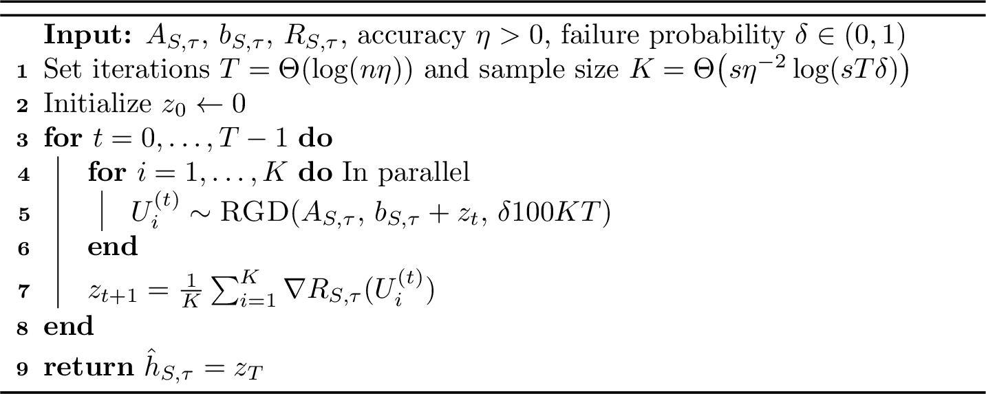
In [alg:parallel-ising-rejection-sampler], \((X,Z)\) corresponds to \((U_\ell,V_\ell)\), both of which are approximately distributed as \(\pi_{S,\tau}\) (modulo the negligible sampling error of [alg:rgd-ising-parallel], which we ignore for now). Since \(\tfrac{d\mu_{S,\tau}}{d\pi_{S,\tau}}(y) \propto e^{\psi(y)}\), where \(\psi(y) = R_{S,\tau}(y) - \langle \hat{h}, y\rangle\), 6 suggests that we can bound the TV error of [alg:parallel-ising-rejection-sampler] by controlling the sampling error of [alg:rgd-ising-parallel] and proving a subexponential tail bound for \(|\psi(\widetilde{U})-\psi(\widetilde{V})|\), where \(\widetilde{U},\widetilde{V} \stackrel{\mathrm{iid}}{\sim} \pi_{S,\tau}\), or equivalently, for \(|\psi(Y)-\mathbb{E}[\psi(Y)]|\) under \(Y \sim \pi_{S,\tau}\). Now, by 5 and 10, \(\pi_{S,\tau}\) satisfies \(\frac{4}{3}\)-ATE with high probability. Thus, 4 gives us the following concentration bound: \[\begin{align} \mathbb{P}_{Y \sim\pi_{S,\tau}}\left[|\psi(Y) - \mathbb{E}_{\pi_{S,\tau}}[\psi(Y)]|\right] \leq 2 \exp(-c \min\{\frac{t^2}{\mathbb{E}_{\pi_{S,\tau}}[\|\nabla \psi\|^2]}, \frac{t}{\max\limits_{y \in \{\pm 1\}^S} \|\nabla^2 \psi(y)\|_F} \}) \end{align}\] Since \(\|\nabla^2 \psi(y)\|^2_F = \|\nabla^2 R_{S,\tau}(y)\|_F \lesssim \mathfrak{C}(\beta) \cdot \tfrac{s^3}{n^2}\) holds whp uniformly for any \(S,\tau\) and \(y\) by 11. Hence, setting \(s = \Theta(n^{\frac{2}{3}})\) and \(\mathfrak{C}(\beta)\) sufficiently small, \(\max\limits_{y \in \{\pm 1\}^S} \|\nabla^2 \psi(y)\|_F \leq \delta\) for any \(\delta = O(1)\). To control \(\mathbb{E}_{\pi_{S,\tau}}[\|\nabla \psi\|^2]\), we note that: \[\begin{align} \label{eq:mean-decomposition} \mathbb{E}_{\pi_{S,\tau}}[\|\nabla \psi\|^2] = \| \;\hat{h} - \mathbb{E}_{\pi_{S,\tau}}[\nabla R_{S,\tau}] \;\|^2 + \mathbb{E}_{\pi_{S,\tau}}\left[\| \;\nabla R_{S,\tau} - \mathbb{E}[\nabla R_{S,\tau}] \;\|^2\right] \end{align}\tag{35}\] Using the Poincare Inequality for \(\pi_{S,\tau}\) and 11, the second term in 35 can be made \(O(\delta^2)\) for any \(\delta = O(1)\) by setting \(s=\Theta(n^{\frac{2}{3}})\) and \(\mathfrak{C}(\beta)\) sufficiently small. The centering field \(\hat{h}\) must be chosen so as to make the first term \(\|\hat{h} - \mathbb{E}_{\pi_{S,\tau}}[\nabla R_{S,\tau}]\|^2\) as small as possible. Since \(\pi_{S,\tau} = \nu_{A_{S,\tau},\, b_{S,\tau}+\hat{h}}\) where \(\nu_{J,v}(y) \propto \exp(\frac{1}{2}\langle y, Jy\rangle + \langle v, y\rangle),\) the optimal choice of \(\hat{h}\) is given by the solution to the following fixed point problem: \[\begin{align} \label{eq:centering-fixed-point} h = \mathbb{E}_{\nu_{A_{S,\tau},\, h + b_{S,\tau}}}[\nabla R_{S,\tau}]. \end{align}\tag{36}\]

As we shall demonstrate, 36 admits a unique solution which can be efficiently approximated by an inexact fixed point iteration, namely 1, which replaces the expectation in 36 by an empirical average over approximate samples drawn via RGD. In particular, we prove the following guarantee in 3.5

3.3.1 Proof of 12↩︎

3.4 Proof of 7↩︎

3.5 Proof of 13↩︎

For any choice of \((S,\tau)\), define the measure \(\gamma_z\) on \(\{\pm 1\}^s\) as \(\gamma_z(y) \propto \exp\Bigl(\tfrac{1}{2}\langle y, A_{S,\tau} y\rangle + \langle b_{S,\tau} + z, y\rangle\Bigr).\) Since we condition on the event \(\mathcal{E}\), \(\|A_{S,\tau}\|_{\mathsf{op}} \leq \tfrac{1}{4}\). Thus, by 5, \(\gamma_z\) satisfies LSI with constant \(4/3\) for any \(z \in \mathbb{R}^s\). Moreover, setting \(s = O(n^{2/3})\) and \(\mathfrak{C}(\beta) = O(1)\) sufficiently small, one can set \(\sup_{y \in \{\pm 1\}^s} \|\nabla^2 R_{S,\tau}(y)\|_F \leq \tfrac{1}{100}.\) Now, define \(F : \mathbb{R}^s \to \mathbb{R}^s\) as follows: \[\begin{align} F(z) = \mathbb{E}_{\gamma_z}\bigl[\nabla R_{S,\tau}(y)\bigr] = \frac{\sum_{y \in \{\pm 1\}^s} \nabla R_{S,\tau}(y)\exp\bigl(\tfrac{1}{2}\langle y, A_{S,\tau} y\rangle + \langle b_{S,\tau}+z, y\rangle\bigr)}{\sum_{y \in \{\pm 1\}^s} \exp\bigl(\tfrac{1}{2}\langle y, A_{S,\tau} y\rangle + \langle b_{S,\tau}+z, y\rangle\bigr)}. \end{align}\] Taking derivatives with respect to \(z\) and rearranging terms, \[\begin{align} \nabla F(z) = \mathbb{E}_{\gamma_z}\bigl[\nabla R_{S,\tau}(y) y^\top\bigr] - \mathbb{E}_{\gamma_z}\bigl[\nabla R_{S,\tau}(y)\bigr]\mathbb{E}_{\gamma_z}\bigl[y^\top\bigr]. \end{align}\] Consider any unit vectors \(u,v \in \mathbb{R}^s\). Then, by Cauchy–Schwarz and the Poincaré inequality for \(\gamma_z\), \[\begin{align} u^\top \nabla F(z) v = \mathrm{Cov}_{\gamma_z}\bigl(\langle u,\nabla R_{S,\tau}\rangle,\langle v,y\rangle\bigr) \leq \sqrt{ \mathrm{Var}_{\gamma_z}\bigl[\langle u,\nabla R_{S,\tau}\rangle\bigr] \mathrm{Var}_{\gamma_z}\bigl[\langle v,y\rangle\bigr] } \leq \frac{4}{3} \sqrt{ \mathbb{E}_{\gamma_z}\bigl[\langle u,\nabla^2 R_{S,\tau}(y)u\rangle\bigr] } < \frac{1}{4}. \end{align}\] Since \(\|\nabla F(z)\|_{\mathsf{op}} < \tfrac{1}{4}\), by the Banach fixed point theorem, there exists a unique \(h^*\) satisfying the following fixed point iteration: \[\begin{align} h^* = F(h^*) = \mathbb{E}_{\gamma_{h^*}}\bigl[\nabla R_{S,\tau}(y)\bigr]. \end{align}\]

Recall that for \(t \in \{0,\ldots,T-1\}\), \(z_{t+1} = \frac{1}{K}\sum_{i=1}^K \nabla R_{S,\tau}\bigl(U_i^{(t)}\bigr),\) where \(U_i^{(t)} = \mathrm{RGD}\Bigl(A_{S,\tau},\, b_{S,\tau}+z_t,\, \tfrac{\delta}{100KT}\Bigr).\) Thus, by 9, there exist \(Y_i^{(t)} \stackrel{\mathrm{iid}}{\sim} \gamma_{z_t}\) such that the following holds with probability at least \(1-\delta\): \[\begin{align} U_i^{(t)} = Y_i^{(t)} \qquad \forall\, t<T,\;i \in [K]. \end{align}\] Henceforth, we condition on this event, so that \(z_{t+1} = \tfrac{1}{K}\sum_{i=1}^K \nabla R_{S,\tau}\bigl(Y_i^{(t)}\bigr)\). Since \(\|\nabla^2 R_{S,\tau}\|_F \leq \tfrac{1}{100}\) and \(\gamma_{z_t}\) satisfies LSI with constant \(4/3\), the following holds by Theorem C and a union bound over \(j \in S\): \[\begin{align} \mathbb{P}\Bigl[ \Bigl\| \frac{1}{K}\sum_{i=1}^K \nabla R_{S,\tau}\bigl(Y_i^{(t)}\bigr) - \mathbb{E}_{\gamma_{z_t}}\bigl[\nabla R_{S,\tau}\bigr] \Bigr\| \geq u \Bigr] \leq 2s e^{-cKu^2/s}. \end{align}\] Setting \(u = \frac{3\eta}{16\sqrt{s}}, K = \Theta\bigl(s\eta^{-2}\ln(sT/\delta)\bigr),\) and taking a union bound over \(t<T\), we conclude that the following holds with probability at least \(1-\delta/2\): \[\begin{align} \|z_{t+1} - F(z_t)\| \leq \frac{3\eta}{16} \qquad \forall\, t<T. \end{align}\]

Let \(\Delta_t = \|z_t - h^*\|.\) Since \(F(h^*) = h^*\) and \(F\) is \(1/4\)-Lipschitz, \[\begin{align} \Delta_{t+1} = \|z_{t+1} - h^*\| = \|z_{t+1} - F(z_t) + F(z_t) - F(h^*)\| \leq \frac{1}{4}\Delta_t + \frac{3\eta}{16}. \end{align}\] Unrolling the recurrence, \[\begin{align} \Delta_T \leq 4^{-T}\Delta_0 + \frac{\eta}{4}. \end{align}\] Since \(z_0 = 0\) and \(\|\nabla R_{S,\tau}\|_\infty \leq n^{\Theta(1)}\) when conditioned on the event \(\mathcal{E}\), \[\begin{align} \|\Delta_0\| = \|h^*\| = \|F(h^*)\| = \Bigl\| \mathbb{E}_{\gamma_{h^*}}\bigl[\nabla R_{S,\tau}\bigr] \Bigr\| \leq n^{\Theta(1)}. \end{align}\] Setting \(T = \Theta\bigl(\ln(n/\eta)\bigr)\) suffices to ensure \(\Delta_T \leq \frac{\eta}{2}.\). Finally, since \(\hat{h} = z_T\), we have \(\|\hat{h} - h^*\| \leq \frac{\eta}{2}\) which then implies the following: \[\begin{align} \Bigl\| \hat{h} - \mathbb{E}_{\pi_{S,\tau}}\bigl[\nabla R_{S,\tau}\bigr] \Bigr\| = \Bigl\| \hat{h} - \mathbb{E}_{\gamma_{\hat{h}}}\bigl[\nabla R_{S,\tau}\bigr] \Bigr\| = \|\hat{h} - F(\hat{h})\| \leq \|\hat{h} - h^*\| + \|F(\hat{h}) - F(h^*)\| \leq \eta. \end{align}\] To analyze the parallel runtime and work, note that 1 runs for \(T\) iterations and each iteration performs \(K\) parallel calls to [alg:rgd-ising-parallel] with error tolerance \(\tfrac{\delta}{100KT}\). Hence, by Theorem 9, 1 has a parallel runtime of \(O(\mathrm{polylog}(n, \eta^{-1}, \delta^{-1}))\) with \(O\bigl(\poly(\tfrac{n}{\eta},\ln(\frac{1}{\delta}))\bigr)\) work.

4 Low Accuracy Parallel Sampler for the \(p\)-Spin Model↩︎

In this section, we prove that Picard Algorithmic Stochastic Localization ([alg:picard-asl]) samples from the mixed \(p\)-spin model with Wasserstein guarantees.

We first illustrate our results for the SK model, a special case of the \(p\)-spin model, because the analysis is simpler and the calculations are closely related. Moreover, for the SK model, we obtain a parallelization result for a broader range of temperatures than the best previous parallel algorithm of [15].

The TAP-AMP mean-estimation algorithm for the SK model ([alg:mean-of-tilted-gibbs-measure-sk]) is slightly different from that for the mixed \(p\)-spin model, but it uses the same AMP iterations followed by NGD iterations. We prove that the TAP-AMP algorithms proposed in prior work for computing mean approximations in the SK and mixed \(p\)-spin models, [alg:mean-of-tilted-gibbs-measure-sk] and [alg:tap-amp], are Lipschitz with respect to the external field and \(\widetilde{O}(1)\) parallel computable. This enables us to apply Picard iteration to the steps of algorithmic stochastic localization 5 , yielding a parallel speedup.

For the rest of the section, we first present an improved parameter dependence for algorithmic stochastic localization in 4.1. Then, using the improved parameters, we prove the parallelization result for algorithmic stochastic localization in 4.2, relying on the following two results:

• The TAP-AMP mean approximations are executable in \(\widetilde{O}(1)\) parallel time (4.3).

• The TAP-AMP mean approximations are Lipschitz (4.4).

4.1 Sign Rounding for Algorithmic Stochastic Localization↩︎

[12], [21] provide Wasserstein guarantees for algorithmic stochastic localization using TAP fixed points as mean approximations. Their analysis controls the propagation of the mean-estimation error along the discretized stochastic localization trajectory. They obtain an \(\varepsilon\) upper bound in normalized Wasserstein distance between the output of the sampling algorithm and the target distribution by using \(\exp(\poly(1/\varepsilon))\) discrete steps to run the stochastic localization up to a time horizon \(\poly(1/\varepsilon)\).

In this work, in addition to the Picard parallelization and Lipschitz analysis, we improve the dependence of the discretization step size and the time horizon in stochastic localization on the parameter \(\varepsilon\) by analyzing sign rounding for algorithmic stochastic localization.

4.2 Parallel Time Analysis of [alg:picard-asl]↩︎

In this section, we analyze the parallelization result for algorithmic stochastic localization using Picard iteration. The Picard iterations produce a trajectory that is close, in Wasserstein distance, to the true solution of the discrete stochastic localization process using the TAP-AMP mean approximation. This discrete process is itself close to the true continuous-time stochastic localization process by 14. Therefore, by the triangle inequality for Wasserstein distance, the input to the rounding step is close to the output of the true stochastic localization process.

However, in our proposed algorithm ([alg:picard-asl]), the final output is obtained by applying the sign function. It is not immediate that small Wasserstein distance before rounding implies small Wasserstein distance after rounding. Indeed, if two coordinates are both close to zero but have opposite signs, applying the sign function can amplify their discrepancy. To address this issue, we use the stability result for sign rounding in 2. This lemma shows that once the Picard trajectory is sufficiently close to the true stochastic localization trajectory, the corresponding sign-rounded outputs remain close in normalized Wasserstein distance.

We present our results for the SK model and the mixed \(p\)-spin model separately. For the SK model, the Gibbs measure is defined by \[\mu_A(x) \propto \exp\left(\frac{\beta}{2}\langle x,Ax\rangle\right),\] where \(A \sim \mathrm{GOE}(n)\). Here \(\mathrm{GOE}(n)\) denotes the distribution over symmetric matrices whose entries are Gaussian with variance of order \(1/n\). Although the proof structure is nearly the same, we separate the two cases because, for the SK model, we obtain a parallel sampling algorithm in a temperature regime not covered by previous parallel algorithms. The analysis for the SK model yields the threshold \(\beta_0 \approx 0.3753\) for Lipschitzness and parallelization, improving on the \(\beta < 1/4\) threshold at which the previous \(\mathrm{polylog}(n)\)-depth algorithm for sampling from the SK model applies [15]. However, unlike the algorithm of [15], our low-accuracy algorithm cannot achieve arbitrarily small error.

4.3 TAP-AMP in \(\mathrm{polylog}(n)\) Parallel Time↩︎

The TAP-AMP mean-approximations can be computed in \(\mathrm{polylog}(n/\varepsilon)\) parallel depth. The TAP-AMP algorithms [alg:mean-of-tilted-gibbs-measure-sk] and [alg:tap-amp] consist of AMP iterations followed by NGD iterations. Each individual AMP or NGD iteration is computable in parallel with depth \(O(\log n)\); thus, it suffices to prove \(\widetilde{O}(1)\) bounds on the numbers of AMP and NGD iterations. Since this proof is rather involved and does not affect the rest of the argument, we give only a brief sketch here and defer the details to the appendix; see 6.

4.4 Lipschitz Property of the TAP-AMP Mean Approximation for the SK Model↩︎

In this section, we prove that, for the SK model at high temperature \(\beta < \beta_0 \approx 0.3753\), the TAP-AMP algorithm ([alg:mean-of-tilted-gibbs-measure-sk]) for mean approximation is \(O\!\left(\frac{1}{\beta_0-\beta}\right)\)-Lipschitz with respect to the tilt parameter, or external field, with high probability. We provide an analogous result for the mixed \(p\)-spin model in 7.

[alg:mean-of-tilted-gibbs-measure-sk] consists of two phases: it first uses AMP iterations attempting to get close to the fixed point of the TAP iteration, and then it uses an NGD algorithm to close the gap to the fixed point as much as needed. Here, we will take a closer look at the two phases of [alg:mean-of-tilted-gibbs-measure-sk].

4.4.0.1 Phase 1: AMP phase.

In the first phase, initialize \[m_{-1}=0,\qquad z_0=0,\] and for \(k=0,1,\dots,K_{\mathrm{AMP}}-1\) define \[\begin{align} m_k &= \tanh(z_k), \tag{42}\\ b_k &= \frac{\beta^2}{n}\sum_{i\in[n]}\mathop{\mathrm{sech}}^{2}\!\bigl((z_k)_i\bigr), \tag{43}\\ z_{k+1} &= \beta A m_k + y - b_k\, m_{k-1}. \tag{44} \end{align}\]

4.4.0.2 Phase 2: NGD phase on TAP free energy.

Initialize \(u_0 := z_{K_{\mathrm{AMP}}}\). For \(t=0,1,\dots,K_{\mathrm{NGD}}-1\) define \[\begin{align} m_t^+ &= \tanh(u_t), \tag{45}\\ u_{t+1} &= u_t - \eta \,\nabla_m \hat{\mathscr{F}}_{\mathrm{TAP}}(m_t^+;y,q). \tag{46} \end{align}\] The algorithm outputs \[\hat{m}(A,y) := m_{K_{\mathrm{NGD}}}^+ = \tanh(u_{K_{\mathrm{NGD}}}).\]

Our goal in this section is to find the temperature \(\beta(A) = \beta(\left\lVert A \right\rVert_{\mathrm{op}})\) such that, for any two tilts \(y\) and \(\widetilde{y}\), the TAP fixed point of the Ising model with interaction matrix \(A\) and temperature \(\beta\) satisfies \[\|\hat{m}_{(K_{\mathrm{AMP}}, K_{\mathrm{NGD}})}(A, y) - \hat{m}_{(K_{\mathrm{AMP}}, K_{\mathrm{NGD}})}(A, \widetilde{y})\| \leq \frac{\gamma({A})}{\beta({A}) - \beta}\norm{y-\widetilde{y}}.\] Note that if the matrix \(A\) is sampled from the \(\mathrm{GOE}(n)\) distribution, then its maximum eigenvalue concentrates around \(2\); thus, if we have inverse temperature \(\beta\) satisfying \(\gamma(2,\beta)< 1\), then we have the Lipschitz property for the TAP-AMP mean approximation \(\hat{m}\) with high probability.

To prove the Lipschitz property of the mean-approximation algorithm ([alg:mean-of-tilted-gibbs-measure-sk]), we will use the Lipschitz property of the following two functions:

• \(\tanh\) is \(1\)-Lipschitz (4).

• \(\mathop{\mathrm{sech}}^{2}\) is \(\frac{4}{3\sqrt{3}}\)-Lipschitz (5).

We will prove that the AMP and NGD iterations are both Lipschitz. Throughout the rest of this section, we fix two external fields \(y\) and \(\widetilde{y}\) and use the following notation, where the unadorned variables correspond to the computation of \(\hat{m}_{(K_{\text{AMP}}, K_{\text{NGD}})}(A, y)\) and the tilded variables correspond to the computation of \(\hat{m}_{(K_{\text{AMP}}, K_{\text{NGD}})}(A, \widetilde{y})\):

• \(\Delta y := y-\widetilde{y}\) (tilt difference)

• \(\Delta z_k := z_k-\widetilde{z}_k\) (AMP iterations)

• \(\Delta m_k := m_k-\widetilde{m}_k\) (AMP iterations)

• \(\Delta u_k := u_k - \widetilde{u}_k\) (NGD iterations)

Also, \(\Delta z_0=\Delta z_{-1}=0\) and \(m_{-1}=\widetilde{m}_{-1}=0\) for the initialization.

Lipschitzness of the full AMP+NGD algorithm for the SK model↩︎

We have proved so far that after an arbitrary number of iterations, \(\norm{\Delta m_k}\) is upper bounded by \(\frac{1}{1 - \gamma(A, \beta)}\norm{\Delta y}\). Now, we prove that applying NGD after AMP preserves the same bound for the difference of the mean estimates. For convenience, and to avoid overloading the notation \(m_k\) from the AMP phase, we analyze the NGD step in the variables \(u_i\) defined by \(m=\tanh(u)\) (equivalently \(u=\mathop{\mathrm{atanh}}(m)\) component-wise).

4.4.0.3 Rewriting the gradient of TAP in \(u\)-space.

The TAP equation is slightly different for the SK model than for the mixed \(p\)-spin model. For a prescribed overlap parameter \(q\), the SK TAP free energy satisfies \[\begin{align} \nabla \mathscr{F}_{\mathrm{TAP}}(m;y,q) = -\beta A m-y+\operatorname{arctanh}(m)+\beta^2(1-q)m. \label{eq:tap-for-sk} \end{align}\tag{48}\]

Plugging \(m=\tanh(u)\) into 48 gives \[\begin{align} \nabla_m \hat{\mathscr{F}}_{\mathrm{TAP}}(\tanh(u);y,q) &= -\beta A\tanh(u) - y + u + \beta^2(1-q)\tanh(u)\nonumber\\ &= -\Big(\beta A - \beta^2(1-q)I\Big)\tanh(u) - y + u. \label{eq:grad95u95form} \end{align}\tag{49}\] Define \[B := \beta A - \beta^2(1-q)I.\] Then the NGD update 46 becomes \[\label{eq:u95update} u_{t+1} = (1-\eta)u_t + \eta\, B\tanh(u_t) + \eta\, y.\qquad{(2)}\]

5 Sign Rounding Analysis for Algorithmic Stochastic Localization↩︎

In this appendix, we show the improved parameter dependence for Algorithmic Stochastic Localization (ASL) using the notation of [alg:picard-asl] and the low-accuracy discussion in the introduction. We use \[K \quad \text{for the number of localization steps}, \qquad \delta \quad \text{for the discretization step size},\] so that the localization time horizon is \(K\delta\).

The accuracy parameter \(\varepsilon\) below is the target error in normalized \(2\)-Wasserstein distance \(W_{2,n}\) from 1. The threshold \(\varepsilon_n=o_n(1)\) is the accuracy threshold of the tilted-mean estimator used in the ASL analysis.

Let \(\widehat m_{t}(y)\) be the TAP-AMP estimate of the tilted mean at localization time \(t\); the dependence on \(t\) enters through the overlap parameter \(q_\star(t)\) in [alg:tap-amp]. The sequential ASL Euler trajectory is \[\widehat y_{(k+1)\delta} = \widehat y_{k\delta} + \delta\,\widehat m_{k\delta}(\widehat y_{k\delta}) + \bigl(B_{(k+1)\delta}-B_{k\delta}\bigr), \qquad \widehat y_0=0,\] or equivalently, with \(w_{k+1}=(B_{(k+1)\delta}-B_{k\delta})/\sqrt{\delta} \sim \mathcal{N}(0,I_n)\), \[\widehat y_{(k+1)\delta} = \widehat y_{k\delta} + \delta\,\widehat m_{G,k\delta}(\widehat y_{k\delta}) + \sqrt{\delta}\,w_{k+1}.\]

Define the normalized trajectory and mean-estimation errors \[\Delta^y_k := \frac{1}{\sqrt n} \left\|\widehat y_{k\delta}-y_{k\delta}\right\|, \qquad \Delta^m_k := \frac{1}{\sqrt n} \left\| \widehat m_{G,k\delta}(\widehat y_{k\delta}) - m_G(y_{k\delta}) \right\| .\]

6 Parallelization of TAP-AMP Mean Approximation Algorithms↩︎

Here, we prove the \(\widetilde{O}(1)\) parallel-depth claim for the tilted-mean oracle used in 14. We keep the notation of the main body: \(K\) and \(\delta\) denote, respectively, the number of stochastic-localization steps and the discretization step size, while \(K_{\mathrm{AMP}}\) and \(K_{\mathrm{NGD}}\) denote the internal iteration counts of the TAP-AMP tilted mean estimator. The localization horizon is \(t_{\varepsilon}=K\delta\), and by 14 we may take \[T_{\varepsilon}=O\!\left(\log(1/\varepsilon)\right), \qquad \delta=\operatorname{poly}(\varepsilon).\] The overlap parameter in the mixed \(p\)-spin algorithm is denoted by \(q^{\star}(t)\), as in 13 . In the SK specialization we write \(q^{\mathrm{SK}}_\star(\beta,t)\) for the corresponding fixed point in [21]; this avoids overloading the mixed \(p\)-spin notation.

7 Lipschitz Property of the TAP Fixed-Point Computation Algorithm for Mixed \(p\)-Spin Models↩︎

In this section, we prove that, for the mixed \(p\)-spin model at sufficiently high temperature, the TAP fixed-point computation algorithm is Lipschitz with respect to the tilt parameter \(y\) with high probability. The proof follows the same two-phase structure as in the SK case: first an AMP phase gets close to the TAP fixed point, and then a natural-gradient descent step in the dual variables closes the remaining gap.

We recall the standard notation for the mixed \(p\)-spin glass. First, the Hamiltonian takes the following form: \[\begin{align} \label{eq:p-spin-model-zero-field} H(x) = \sum_{p=2}^{P} \frac{\beta_p \sqrt{p!}}{n^{\tfrac{p-1}{2}}} \cdot \sum_{J \subseteq [n], |J|=p} G_J \;\prod_{k \in J}x_k , \qquad \mu(x) = \frac{1}{Z}\exp(H(x)) \end{align}\tag{50}\] where we assume zero external field. Also recall the associated mixture function \[\xi(t)=\sum_{p=2}^{P} \beta_p^2 t^p \qquad \text{equivalently,} \qquad \mathbb{E}{H_n(x)H_n(x')} = n\xi\left(\frac{\ip{x}{x'}}{n}\right).\] Throughout this section, we condition on the high-probability event that the Hamiltonian has a dimension-free Hessian bound. Namely, for a deterministic constant \(L_H\) depending only on \(\xi\), we condition on the following event: \[\begin{align} \sup_{m\in[-1,1]^n}\norm{\nabla^2 H_n(m)}_{\mathsf{op}}\le L_H. \end{align}\] Using Gaussian concentration (see [51]) one can prove that the above event holds with probability at least \(1-e^{-cn}\).

The TAP fixed-point computation for the \(p\)-spin model is very similar to that for the SK model, but it is more complicated because it uses derivatives of the mixture function. Here, we review the TAP fixed-point computation used in [41].

7.0.0.1 Phase 1: AMP phase.

We have the following initialization: \[m_{-1}=0,\qquad z_0=0.\] For \(k=0,1,\dots,K_{\mathrm{AMP}}-1\), define \[m_k = \tanh(z_k),\] \[q_k = \frac{1}{n}\sum_{i=1}^{n}\tanh^2\bigl((z_k)_i\bigr) =\frac{1}{n}\norm{m_k}^2,\] \[b_k = (1-q_k)\xi''(q_k),\] and \[z_{k+1} = \nabla H_n(m_k)+y-b_km_{k-1}. \]

7.0.0.2 Phase 2: NGD phase on the approximate TAP free energy.

Initialize \[u_0:=z_{K_{\mathrm{AMP}}}.\] For \(t=0,1,\dots,K_{\mathrm{NGD}}-1\), define \[m_t^+ = \tanh(u_t),\] and \[u_{t+1} = u_t-\eta\nabla_m \hat{\mathscr{F}}_{\mathrm{TAP}}(m_t^+;y,q). \] The algorithm outputs \[\widehat m(G,y):=m_{K_{\mathrm{NGD}}}^+=\tanh(u_{K_{\mathrm{NGD}}}).\]

Our goal is to prove that, for any two tilts \(y,\widetilde{y}\in\mathbb{R}^n\), the output satisfies \[\norm{\widehat m(G,y)-\widehat m(G,\widetilde{y})} \le \frac{1}{1-\gamma_{\mathrm{mix}}}\norm{y-\widetilde{y}},\] provided \(\gamma_{\mathrm{mix}}<1\). The proof uses the following elementary Lipschitz facts:

• \(\tanh\) is \(1\)-Lipschitz;

• \(\tanh^2\) is \(L_0=4/(3\sqrt3)\)-Lipschitz;

• \(\phi(t)=(1-t)\xi''(t)\) is \(L_\phi\)-Lipschitz on \([0,1]\).

Throughout the proof, fix two external fields \(y\) and \(\widetilde{y}\). Unadorned variables correspond to the computation with tilt \(y\), and tilded variables correspond to the computation with tilt \(\widetilde{y}\). We use the notation \[\begin{align} \Delta y &:= y-\widetilde{y}, & \Delta z_k &:= z_k-\widetilde{z}_k, & \Delta m_k &:= m_k-\widetilde{m}_k, \\ \Delta q_k &:= q_k-\widetilde{q}_k, & \Delta b_k &:= b_k-\widetilde{b}_k, & \Delta u_t &:= u_t-\widetilde{u}_t. \end{align}\] Also, \(\Delta z_0=0\), \(\Delta z_{-1}=0\), and \(m_{-1}=\widetilde{m}_{-1}=0\) by initialization.

Lipschitzness of the full AMP+NGD algorithm for mixed \(p\)-spin↩︎

We next prove that the NGD phase preserves the AMP Lipschitz bound, up to replacing \(\gamma_{\mathrm{AMP}}\) by the larger stability parameter \(\gamma_{\mathrm{mix}}\).

7.0.0.3 Rewrite the gradient of TAP in \(u\)-space.

We recall several definitions from the preliminaries regarding the TAP equation.

\[\begin{align} \mathscr{F}_{\mathrm{TAP}}(m,y) &= -H(m) - \left\langle y, m \right\rangle - \sum_{i=1}^{n} h(m_i) - \operatorname{ONS}(Q(m)) \\ \operatorname{ONS}(q) &= \frac{n}{2}\left[\xi(1)-\xi(Q)-(1-Q)\xi^{\prime}(Q)\right] \\ \mathrm{ONS}'(q)&=-\frac{n}{2}(1-q)\xi''(q) \\ Q(m) &= n^{-1}\|m\|^2, \qquad h(m) = -\frac{1+m}{2}\ln\left(\frac{1+m}{2}\right) - \frac{1-m}{2}\ln\left(\frac{1-m}{2}\right) \end{align}\] A direct calculation gives \[\begin{align} \nabla_m F_{\mathrm{TAP}}(m;y,q) &= -\nabla H_n(m)-y+\operatorname{arctanh}(m) +(1-q)\xi''(q)m\\ &\quad +\frac{T}{2}\bigl(Q(m)-q\bigr)m. \end{align}\] Plugging in \(m=\tanh(u)\) gives \[\nabla_m F_{\mathrm{TAP}}(\tanh(u);y,q)=u-y-\mathcal{G}(u),\] where \[\mathcal{G}(u) :=\nabla H_n(\tanh(u)) -(1-q)\xi''(q)\tanh(u) -\frac{T}{2}J(\tanh(u)),\] and \[J(m):=\bigl(Q(m)-q\bigr)m.\] Thus the NGD update [eq:mixed-ngd-update] becomes \[u_{t+1}=(1-\eta)u_t+\eta y+\eta\mathcal{G}(u_t). \]

8 \(\exp(\poly(1/\varepsilon))\) Steps for Algorithmic Stochastic Localization↩︎

References↩︎

---

1. As explained in 3.3, the nonzero external field \(\hat{h}\) centers our rejection sampling proposal, leading to improved accuracy.↩︎