A hybrid analytical-PINN model for subsurface simulation of geothermal heat exchangers in heterogeneous underground
July 14, 2026
In this paper, a parametric physics-informed neural network for solving the heterogeneous soil thermal problem with borehole heat exchangers (BHEs) as singular sources is developed. There are three novel features in the present framework; namely, (i) the singularity is naturally removed by using analytical line source models; (ii) using the explicit formulation for gradient thermal conductivity enables physics-informed learning of the parametrization featuring the conductivity; (iii) the learned correction is utilized as an efficient universal corrector via superposition principles. We first introduce the decomposition of the temperature change and transform the approximation of the entire heterogeneous response to the correction compensating the difference between the practical solution and idealized homogeneous approximation. In such a way, the delta function singularity is excluded and the bulk heat transfer is captured for the sake of facilitating the effective training of the neural network. The original problem is then reformulated as a governing correction diffusion or advection-diffusion equation subject to a homogeneous initial condition. The linearly varying thermal conductivity is used to model the soil heterogeneity. We propose a physics-informed neural network to approximate a universal corrector with respect to a single borehole with unit heat extraction rate. As a result, the network is trained by minimizing the physics-informed and data-anchored loss function that is evaluated for sampled conductivity parameters on adaptively selected training points. In addition, we include the location indicator function regarding the source as a feature input of network and find that it helps the network to process the local information. We perform numerical tests to exhibit the effectiveness of the proposed method based on the infinite line source (ILS), finite line source (FLS) and moving finite line source (MFLS) models.
Keywords: Shallow geothermal energy, Borehole heat exchanger, Physics-informed neural networks, Analytical correction, Heterogeneous media
1 Introduction↩︎
Decarbonizing heating and cooling is a central component of the transition toward low-carbon energy systems [1], [2]. Shallow geothermal energy, commonly utilized through ground-source heat-pump systems, provides a locally available and seasonally stable thermal resource for building thermal conditioning and underground thermal-energy storage [3]–[5]. Among the available ground heat exchanger configurations, vertical borehole heat exchangers (BHE) are particularly attractive. A BHE circulates a heat-carrier fluid through closed pipes installed in a vertical borehole and exchanges heat with the surrounding ground without directly extracting groundwater [6]. Its long-term performance depends strongly on the transient thermal response of the subsurface and on the thermal interaction among neighboring boreholes [7], [8].
Accurate and repeated forward simulation of the ground temperature field is therefore essential for the design and operation of BHE systems [9], [10]. A broad range of analytical and semi-analytical models have been developed for BHE simulation, including infinite line source, finite line source and moving finite line source models [11]–[13]. They represent a borehole as a line source and provide physically interpretable descriptions of the radial transient response. However, their computation efficiency is obtained at the expense of restrictive assumptions, such as idealized homogeneous and infinite ground domain, simplified boundary conditions and spatially uniform groundwater velocity [14]. On the other hand, numerical methods provide greater flexibility and can resolve more complex soil properties, geometries and subsurface transport conditions [15]–[17]. Over the last decades, a variety of specialized numerical solvers for BHE simulation have been developed by dimensional reduction and hybrid formulation, including TRNSYS [18], OpenGeoSys [19] and FEFLOW [20]. However, long-term three-dimensional numerical simulations remain computationally prohibitive, especially for repeated evaluations under varying configurations and operating conditions [21].
Applying deep neural networks to repeated BHE and subsurface thermal simulation has thus drawn much attention recently. A trained neural surrogate can predict temperature fields at a substantially lower online cost compared to numerical simulation and especially benefits any procedure requiring numerous simulation runs. In terms of training mechanism, the data-driven and physics-informed neural networks define the loss based on different sources of information. The quality and quantity of training samples largely determine the performance of the purely data-driven models. In contrast, physics-informed neural networks (PINNs) augment the learning process by introducing governing partial differential equations (PDEs), initial conditions and boundary conditions into the training objective [22]. Consequently, the use of physical constraints can reduce the expensive data generation burden, allow differentiable approximations over the space-time domain and enhance the generalization ability outside the sampled parameter range. These properties make PINNs attractive as reusable thermal simulators for BHE systems in heterogeneous media. However, their utilization in the field is still lacking due to the challenging nature of the singular (BHE) sources [23].
Solving PDEs with singular sources is challenging for standard DNNs and vanilla PINNs since they lack the expressive power to effectively approximate the solution containing a highly localized singularity. Therefore, several developments for physics-informed neural solvers have been proposed to deal with the nonsmoothness of PDE solution. Gao et al. [24] proposed a failure-informed adaptive sampling strategy that places additional collocation points in regions with large residual-based failure probabilities. This is further combined with re-sampling and subset simulation to improve the detection of localized high-error regions in [25]. Adaptive sampling is also adapted in [26] where the localized source is represented by a normalized Gaussian profile. Whereas in terms of approximating point sources, Huang et al. use a continuous probability density and combine this regularization with an uncertainty-based loss weighting strategy and a practical multiscale neural architecture in [27]. Making use of the separation of the singularity from the network approximation target, [28] proposed a singularity-splitting deep Ritz method that represents the known singular component analytically and trains the neural network only for the regular remainder. Furthermore, Hu et al. [29] developed a singularity-enriched PINN that explicitly incorporates explicit singular basic functions for Poisson problems to construct a more expressive approximation space of PINN. Later this framework was extended to solving inverse problems by jointly identifying the locations and intensities of unknown point sources. [30] handle elliptic problems with singular sources on an interface by formulating the variational problem and use level set function to give the network additional information about the interface.
In this paper, adopting the idea that localized singularities can be extracted by analytical solution, we propose a parametric hybrid PINN method for solving the soil temperature simulation problem with singular line sources (BHEs). The contributions of the proposed method are three-fold. First, we exclude the delta function singularity embedded in the source terms by using analytical solutions as base models. Second, we target the linearly changing thermal conductivity cases, which allows training the network with physics-informed loss and generalization to unseen gradient conductivity scenarios. Third, the parametric neural network is trained on various sampled conductivity conditions to approximate the temperature correction induced by a singular borehole at the origin with unit heat transfer rate, which could be employed as a computationally efficient universal corrector by applying superposition principle. This helps avoid training different networks for diverse arrangements of BHEs and source load profiles. In addition, we rewrite the governing equation into a formulation on relative coordinates with respect to the borehole location, and then the network learns the output only considering the distance from the source under a certain thermal conductivity in an open-boundary domain. We thus include the distance from the borehole as input feature of the network that effectively improves the simulation accuracy near the source.
The rest of the paper is organized as follows. Section 2 introduces the classical formulations for the global soil temperature model problem. In Section 3, the parametric hybrid-PINN universal corrector method to simulate the models is presented. In Section 4, we test and compare several numerical examples concerning ILS, FLS and MFLS analytical models, followed by conclusions of the present method and future work directions in Section 5.
2 Problem Formulation↩︎
Looking into the transient propagation of temperature perturbations in the subsurface induced by a field of BHEs, we consider the global thermal problem as the evolution of the soil temperature field around the BHEs. Assume \(\Omega_s\) denotes the soil domain and \(I=\left(0,T\right)\) is the time interval of interest. The soil temperature \(T\left(\mathbf{x},t\right)\), \(\mathbf{x}\in \Omega_s\), \(t\in I\) in a heterogeneous porous medium is governed by the combined effects of thermal diffusion and groundwater advection. We first consider the conduction-dominated case \[\begin{align} \rho_s C_s\frac{\partial T}{\partial t} -\nabla \cdot \left( \lambda(\mathbf{x}) \nabla T \right) =f\left(\mathbf{x},t\right),\label{eq:conduction95soil95model} \end{align}\tag{1}\] where \(\rho_s C_s\) is the volumetric heat capacity of the soil and \(\lambda(\mathbf{x})\) denotes the thermal conductivity of the soil. Hence the temperature change \(\widetilde{T}\left(\mathbf{x},t\right)=T\left(\mathbf{x},t\right)-T_u\) relative to the undisturbed constant ground state \(T_{u}\) follows the same mechanism \[\begin{align} \rho_s C_s\frac{\partial \widetilde{T}}{\partial t} -\nabla \cdot \left( \lambda(\mathbf{x}) \nabla \widetilde{T} \right) =f\left(\mathbf{x},t\right).\label{eq:conduction95soil95change95model} \end{align}\tag{2}\] Taking the groundwater flow effect into account, BHE-induced temperature change satisfies the advection-diffusion equation \[\rho C \frac{\partial \widetilde{T}}{\partial t} + \rho_fC_f \mathbf{v}\cdot \nabla \widetilde{T} - \nabla \cdot \left( \lambda(\mathbf{x}) \nabla \widetilde{T} \right) = f(\mathbf{x},t), \label{eq:advection95conduction95soil95model}\tag{3}\] where \(\rho C\) is the combined volumetric heat capacity of the solid and liquid phase, i.e., \(\rho C=\epsilon \rho_f C_f +\left(1-\epsilon\right)\rho_s C_s\), \(\rho_f c_f\) is the volumetric heat capacity of groundwater and \(\mathbf{v}\) is the Darcy velocity of the groundwater flow.
Furthermore, \(f\left(\mathbf{x},t\right)\) represents the heat source or sink induced by BHE operation. For a field of \(K\) vertical boreholes, the heat source term can be written as a superposition of individual borehole sources, \[f(\mathbf{x},t) = \sum_{k=1}^{K} f_k(\mathbf{x},t), \notag\] where \(f_k\) denotes the source term associated with the \(k\)-th borehole. Let \(\mathbf{x}^k=(x_{BHE}^k,y_{BHE}^k)\) be the location of the \(k\)-th borehole in the horizontal plane and \(q_k(t)\) be the heat injection or extraction rate per unit length. The infinite line source idealizes the borehole as an infinitely long vertical source and writes \[f_k^{\mathrm{ILS}}(\mathbf{x},t) = q_k(t)\, \delta(x-x_{BHE}^k)\delta(y-y_{BHE}^k), \label{eq:ils95source}\tag{4}\] where \(\delta(\cdot)\) is the Dirac delta distribution.
A more realistic representation accounts for the finite borehole length \(L\). If the borehole extends from the depth \(z=D\) to the depth \(z=D+L\), the finite line source term reads \[f_k^{\mathrm{FLS}}(\mathbf{x},t) = q_k(t)\, \delta(x-x_{BHE}^k)\delta(y-y_{BHE}^k) \chi_{[D,D+L]}(z), \label{eq:fls95source}\tag{5}\] where \(\chi_{[0,L]}(z)\) is the indicator function along the borehole depth.
The temperature field is initialized from the undisturbed state \[T(\mathbf{x},0)=T_u,\quad \mathbf{x}\in\Omega_s, \notag\] and here we assume a constant temperature Dirichlet boundary condition is imposed on \(\partial\Omega_s\) for (1 ), \[T(\mathbf{x},t)=T_u,\quad \mathbf{x}\in\partial\Omega_s,\;t\in I . \notag\] Equivalently, for the temperature change \(\widetilde{T}\), these conditions are enforced as \[\widetilde{T}(\mathbf{x},0)=0,\quad \mathbf{x}\in\Omega_s,\label{eq:initial95Ttilde}\tag{6}\] and for (2 ) \[\widetilde{T}(\mathbf{x},t)=0,\quad \mathbf{x}\in\partial\Omega_s,\;t\in I. \label{eq:boundary95Ttilde}\tag{7}\]
In this work, we focus on a heterogeneous setting in which the soil thermal conductivity is modeled as a linear gradient field in the horizontal plane \[\lambda(\mathbf{x}) = \lambda_c+\lambda_xx+\lambda_yy, \notag\] where \(\lambda_c\) denotes the conductivity value at the horizontal coordinate origin \(\left(x,y\right)=\left(0,0\right)\) and \(\left(\lambda_x,\lambda_y\right)\) is the constant gradient of spatially varying \(\lambda\left(\mathbf{x}\right)\). The conductivity is assumed to be invariant along the vertical direction. Fully resolved subsurface conductivity fields are rarely available in practical shallow geothermal applications, while standard thermal response tests usually provide only effective or averaged thermal properties. Therefore, the gradient conductivity field is adopted as a controlled representation of commonly encountered BHE system-scale subsurface heterogeneity. Compared with the homogeneous assumption, it captures more realistic subsurface heat transfer characteristics while remaining sufficiently simple for systematic analysis.
3 Hybird-PINN Universal Corrector Method↩︎
3.1 Hybrid PINN Corrector Based on Analytical Models↩︎
We propose a hybrid PINN corrector method for problem (2 ) subject to conditions (6 ), (7 ) and for problem (3 ) with initial condition (6 ) by applying analytical models with respect to source terms (4 ) and (5 ). In this section, we discuss the case with a single source located in \(\Omega_s\) with a unity load rate. The case of multiple boreholes can be handled via linear superposition.
Instead of approximating the entire BHE-induced temperature field, we decompose the temperature change into an analytical base component and a learned correction component \[\widetilde{T}(\mathbf{x},t) = \widetilde{T}^{m}(\mathbf{x},t) + \widetilde{T}_c^{m}(\mathbf{x},t), \qquad m\in\{\mathrm{ILS},\mathrm{FLS},\mathrm{MFLS}\}. \notag\] Here, \(\widetilde{T}^{m}\) denotes the analytical prediction given by the selected line source model, and \(\widetilde{T}_C^{m}\) is the correction field to be approximated by a neural network. By incorporating analytical knowledge of the underlying solution to the problem of interest, the singularity due to the line source could be captured explicitly. The correction component is then introduced to represent the discrepancy between the analytical reference approximation and global heterogeneous solution. We consider three analytical base models depending on whether the groundwater flow and finite borehole length are taken into account.
3.1.0.1 Infinite line source (ILS) model.
For a two-dimensional infinite homogeneous domain, ILS model assumes heat conduction without groundwater advection in the underground and expresses the radial temperature distribution caused by a single BHE subjected to a piecewise constant heat load over \(m\) time steps as \[\widetilde{T}^{\mathrm{ILS}}(x,y,t) = \sum_{l=0}^{m-1} \frac{q_{l}-q_{l-1}}{4\pi\lambda_0} \mathrm{E_1}\!\left( \frac{r^2}{4\alpha_0\left(t-t_{l}\right)} \right), \label{eq:ils95piecewise95load}\tag{8}\] where \(\mathrm{E_1}\left(\cdot\right)\) is the exponential integral, \(r=\sqrt{(x-x_{BHE})^2+(y-y_{BHE})^2}\) is the distance from the BHE centered at \(\left(x_{BHE},y_{BHE}\right)\), \(\lambda_0\) is the bulk thermal conductivity, \(\alpha_0=\lambda_0/\left(\rho_s C_s\right)\) denotes the thermal diffusivity and \(q_l\) is the load during time step from \(t_{l-1}\) to \(t_l\), with \(q_{-1}=0\) and \(t_0=0\) [11]. The corresponding homogeneous heat diffusion equation with respect to ILS solution is \[\rho_s C_s \frac{\partial \widetilde{T}^{\mathrm{ILS}}}{\partial t} - \lambda_0 \Delta \widetilde{T}^{\mathrm{ILS}} =q(t)\delta\left(x-x_{BHE}\right)\delta\left(y-y_{BHE}\right). \label{eq:ils95homogeneous95pde}\tag{9}\]
3.1.0.2 Finite line source (FLS) model.
To evaluate the thermal behavior in a three-dimensional homogeneous domain, FLS model represents the boreholes as line sources of finite lengths and assumes a uniform heat rate per unit length along the borehole, an idealized geometry with zero radius and no groundwater effect on the temperature distribution in the underground [12]. If the borehole extends from the ground surface \(z=D\) to the depth \(z=D+L\), \[\widetilde{T}^{\mathrm{FLS}}(x,y,z,t) = \sum_{l=0}^{m-1} \frac{q_l-q_{l-1}}{4\pi \lambda_0} \int_{D}^{D+L} \frac{ \operatorname{erfc} \!\left[ \dfrac{R(z')}{2\sqrt{\alpha_0\left(t-t_l\right)}} \right] }{R(z')} \,\mathrm dz', \label{eq:fls95piecewise95load}\tag{10}\] where \(\mathrm{erfc}\left(\cdot\right)\) denotes the complementary error function and \(R(z')=\sqrt{r^2+(z-z')^2}\). The corresponding homogeneous equation regarding FLS solution is \[\rho_s C_s \frac{\partial \widetilde{T}^{\mathrm{FLS}}}{\partial t} - \lambda_0 \Delta \widetilde{T}^{\mathrm{FLS}} =q(t) \delta(x-x_{BHE}) \delta(y-y_{BHE}) \chi_{[D,D+L]}(z). \notag\]
3.1.0.3 Moving finite line source (MFLS) model.
The MFLS model extends the FLS solution to a homogeneous medium with groundwater advection governed by a uniform Darcy velocity \(\mathbf{v}=\left(v_x,v_y,0\right)\), which reads \[\widetilde{T}^{\mathrm{MFLS}}(x,y,z,t) = \sum_{l=0}^{m-1} \frac{q_l-q_{l-1}}{8\pi \lambda_0} \int_{0}^{t-t_l} \frac{1}{\tau} \exp \!\left[ - \frac{ (x-v_x\tau)^2+(y-v_y\tau)^2 }{4\alpha'_0\tau} \right] \mathcal{Z}(z,\tau) \,\mathrm d\tau , \label{eq:mfls95piecewise95load}\tag{11}\] where \(\alpha'_0=\lambda_0/\left(\rho C\right)\), \[\mathcal{Z}(z,\tau) = \operatorname{erf} \!\left[ \frac{D+L-z}{2\sqrt{\alpha_0\tau}} \right] - \operatorname{erf} \!\left[ \frac{D-z}{2\sqrt{\alpha_0\tau}} \right], \notag\] and \(\mathrm{erf}\left(\cdot\right)\) denotes the error function [13]. The corresponding homogeneous advection-diffusion equation concerning MFLS solution is \[\rho C \frac{\partial \widetilde{T}^{\mathrm{MFLS}}}{\partial t} + \rho_f C_f \mathbf{v}\cdot \nabla \widetilde{T}^{\mathrm{MFLS}} - \lambda_0 \Delta \widetilde{T}^{\mathrm{MFLS}}=q(t) \delta(x-x_{BHE}) \delta(y-y_{BHE}) \chi_{[D,D+L]}(z). \notag\]
All three analytical models are used here as reference solutions under simplified homogeneous assumptions. They play a key role in removing the dominant singular response so that the remaining correction field can be learned more efficiently by the physics-informed neural network. We now derive the governing equations for \(\widetilde{T}_c^m\), \(m=\{\mathrm{ILS}, \mathrm{FLS}, \mathrm{MFLS}\}\). We illustrate the procedure using \(\widetilde{T}_c^{\mathrm{ILS}}\) as an example, and the deduction for \(\widetilde{T}_c^{\mathrm{FLS}}\) and \(\widetilde{T}_c^{\mathrm{MFLS}}\) can be handled similarly.
Setting \(f\left(\mathbf{x},t\right)=q(t)\delta\left(x-x_{BHE}\right)\delta\left(y-y_{BHE}\right)\) in (2 ) and subtracting (9 ) from it, we have the correction equation \[\rho_s C_s\frac{\partial \widetilde{T}_{c}^{ILS}}{\partial t}-\nabla \cdot\left(\lambda\left(x,y\right)\nabla \widetilde{T}_{c}^{ILS}\right)=\nabla \cdot \left(\left(\lambda\left(x,y\right)-\lambda_0\right)\nabla \widetilde{T}^{ILS}\right),\label{correction95ils}\tag{12}\] where the left-hand side describes the transport of temperature correction and the forcing term represents the heat flow error introduced by plugging the homogeneous solution into the heterogeneous physics \(\lambda\left(\mathbf{x}\right)\). By rewriting \(\lambda\left(\mathbf{x}\right)\) in (12 ) as \(\lambda\left(\mathbf{x}\right)=\lambda_B+\lambda_x x_{rel}+\lambda_y y_{rel}\), where \(\lambda_B=\lambda\left(x_{BHE},y_{BHE}\right)\), \(x_{rel}=x-x_{BHE}\) and \(y_{rel}=y-y_{BHE}\), we obtain \[\begin{align} & \rho_s C_s\frac{\partial \widetilde{T}_{c}^{ILS}}{\partial t}\left(x,y\right) - \lambda_x\frac{\partial \widetilde{T}_{c}^{ILS}}{\partial x}\left(x,y\right) -\left( \lambda_B + \lambda_x x_{rel} +\lambda_y y_{rel}\right) \frac{\partial^2 \widetilde{T}_{c}^{ILS}}{\partial x^2}\left(x,y\right)\notag\\ &- \lambda_y\frac{\partial \widetilde{T}_{c}^{ILS}}{\partial y}\left(x,y\right) -\left( \lambda_B + \lambda_x x_{rel} +\lambda_y y_{rel}\right) \frac{\partial^2 \widetilde{T}_{c}^{ILS}}{\partial y^2}\left(x,y\right)\notag\\ = & \lambda_x\frac{\partial \widetilde{T}^{ILS}}{\partial x}\left(x_{rel},y_{rel}\right) + \left(\lambda_B-\lambda_0 + \lambda_x x_{rel} +\lambda_y y_{rel}\right) \frac{\partial^2 \widetilde{T}^{ILS}}{\partial x^2}\left(x_{rel},y_{rel}\right)\notag\\ &+ \lambda_y\frac{\partial \widetilde{T}^{ILS}}{\partial y}\left(x_{rel},y_{rel}\right) + \left(\lambda_B-\lambda_0 + \lambda_x x_{rel} +\lambda_y y_{rel}\right)\frac{\partial^2 \widetilde{T}^{ILS}}{\partial y^2}\left(x_{rel},y_{rel}\right).\label{showing95coordinates95absolute} \end{align}\tag{13}\] Replacing \(x\) by \(x_{rel}+x_{BHE}\) and \(y\) by \(y_{rel}+y_{BHE}\) in (13 ) and putting the horizontal coordinate origin at the central location of the borehole result in \[\begin{align} & \rho_s C_s\frac{\partial \widetilde{T}_{c}^{ILS}}{\partial t}\left(x_{rel},y_{rel}\right) - \lambda_x\frac{\partial \widetilde{T}_{c}^{ILS}}{\partial x}\left(x_{rel},y_{rel}\right) -\left( \lambda_B + \lambda_x x_{rel} +\lambda_yy_{rel}\right) \frac{\partial^2 \widetilde{T}_{c}^{ILS}}{\partial x^2}\left(x_{rel},y_{rel}\right)\notag\\ &- \lambda_y\frac{\partial \widetilde{T}_{c}^{ILS}}{\partial y}\left(x_{rel},y_{rel}\right) - \left( \lambda_B + \lambda_x x_{rel} +\lambda_yy_{rel}\right) \frac{\partial^2 \widetilde{T}_{c}^{ILS}}{\partial y^2}\left(x_{rel},y_{rel}\right)\notag\\ = & \lambda_x\frac{\partial \widetilde{T}^{ILS}}{\partial x}\left(x_{rel},y_{rel}\right) + \left(\lambda_B-\lambda_0 + \lambda_x x_{rel} +\lambda_y y_{rel}\right) \frac{\partial^2 \widetilde{T}^{ILS}}{\partial x^2}\left(x_{rel},y_{rel}\right)\notag\\ &+ \lambda_y\frac{\partial \widetilde{T}^{ILS}}{\partial y}\left(x_{rel},y_{rel}\right) + \left( \lambda_B -\lambda_0+ \lambda_x x_{rel} +\lambda_y y_{rel}\right) \frac{\partial^2 \widetilde{T}^{ILS}}{\partial y^2}\left(x_{rel},y_{rel}\right).\label{showing95coordinates95relative} \end{align}\tag{14}\] Thus, the solution of (14 ) represents the temperature correction distribution as a function of the relative position with respect to the borehole.
Assuming FLS reference model uses the same source term as the heterogeneous problem and applying a similar procedure to obtaining the correction equation for FLS base solution arrives at \[\rho_s C_s \frac{\partial \widetilde{T}_{c}^{FLS}}{\partial t} - \nabla\cdot \left( \lambda(x,y)\nabla \widetilde{T}_{c}^{FLS} \right) = \nabla\cdot \left( \left(\lambda(x,y)-\lambda_0\right) \nabla \widetilde{T}^{FLS} \right). \label{eq:correction95fls}\tag{15}\] Here, the gradient and divergence operators are taken in three-dimensional space. The same idea leads to the MFLS-based correction equation \[\rho C \frac{\partial \widetilde{T}_{c}^{MFLS}}{\partial t} + \rho_f C_f \mathbf{v}\cdot \nabla \widetilde{T}_{c}^{MFLS} - \nabla\cdot \left( \lambda(x,y)\nabla \widetilde{T}_{c}^{MFLS} \right) = \nabla\cdot \left( \left(\lambda(x,y)-\lambda_0\right) \nabla \widetilde{T}^{MFLS} \right). \label{eq:correction95mfls}\tag{16}\] Via formulating \(\lambda\left(\mathbf{x}\right)\) as \(\lambda_B+\lambda_xx_{rel}+\lambda_yy_{rel}\) in (15 ) and (16 ), the correction equation based on arbitrary analytical base model solves the radial distribution around the line source.
As a result, the ILS, FLS and MFLS corrections embedded in the differential equations obey the same mechanism, where the left-hand side of the equations transport the thermal correction under the target global physics, while the right-hand side provides the residual forcing generated by evaluating a homogeneous analytical prior in a heterogeneous conductivity field. Thus, the neural network does not need to directly deal with the singularity challenge arising from the original problems (2 ) and (3 ).
Since the temperature perturbation satisfies (6 ) and the hybrid decomposition gives \(\widetilde{T}_{c}^{m}=\widetilde{T}-\widetilde{T}^{m}\), \(m\in\{\mathrm{ILS},\mathrm{FLS},\mathrm{MFLS}\}\), the corresponding correction field satisfies the following initial condition \[\widetilde{T}_{c}^{m}(\mathbf{x},0)=0, \quad \mathbf{x}\in \Omega_s, \quad \mathrm{m}\in\{\mathrm{ILS}, \mathrm{FLS}, \mathrm{MFLS}\}.\notag\] On the other hand, the ILS and FLS based corrections mainly consist of the calibration of two physical mismatches: one induced by the imbalance between averaged and variable conductivities and one caused by difference between boundary conditions for infinite and finite domains. Thus, \[\begin{align} \widetilde{T}_{c}^{m}(\mathbf{x},t)=- \widetilde{T}^{m}(\mathbf{x},t), \quad\mathbf{x}\in\partial\Omega_s,\quad t\in I, \quad \mathrm{m}\in\{\mathrm{ILS}, \mathrm{FLS}\}.\notag \end{align}\]
3.2 Boundary Condition Enforcement↩︎
As discussed above, the ILS-based and FLS-based temperature correction fields contain both the correction for mismatch from formation properties and the boundary conditions. The former appears as an interior forcing term in the correction equations, while the latter is inherited from the difference between the idealized boundary assumptions of ILS/FLS models and the prescribed boundary conditions of the original problem. For clarity, we consider a homogeneous finite-domain solution \(T_{h}\) with constant conductivity \(\lambda_0\); then the boundary correction can be defined for \(\mathrm{m}\in\{\mathrm{ILS}, \mathrm{FLS}\}\) as \[B(\mathbf{x},t) =T_h(\mathbf{x},t)-\left(\widetilde{T}^{m}(\mathbf{x},t)+T_u\right) =\widetilde{T}_h(\mathbf{x},t)-\widetilde{T}^{m}(\mathbf{x},t),\notag\] which satisfies a homogeneous heat equation, \[\rho_s C_s \frac{\partial B}{\partial t} - \lambda_0 \Delta B = 0, \qquad \mathbf{x}\in \Omega_s,\quad t\in I, \label{eq:boundary95correction95pde}\tag{17}\] with the inherited boundary condition \[B(\mathbf{x},t)=-\widetilde{T}^m(\mathbf{x},t), \qquad \mathbf{x}\in\partial\Omega_s,\quad t\in I. \label{eq:boundary95correction95bc}\tag{18}\] Thus, the boundary correction is a well-defined component governed by the inconsistency between the boundary conditions.
In a vanilla PINN formulation, the Dirichlet boundary conditions are implemented using additional penalization terms as a contribution to the loss function. However, this treatment is particularly inefficient for the present boundary correction problem (17 ) with (18 ). This difficulty originates from the fact that the line source response is strongly localized near the borehole at early times, while the thermal perturbation gradually propagates across the domain and interacts with the external boundary at later times. This produces a pronounced imbalance in both spatial locations and temporal scales, making the approximation sensitive to the sampling of residual and boundary collocation points. Moreover, statically assigned weights to different loss terms is generally inadequate to accommodate the continuously evolving distribution of the correction field, making the optimization sensitive to hyperparameter tuning and resulting in substantial computational cost. Therefore, for the FLS-based correction equation, we adopt a hard-constrained strategy based on a distance function to match the specified correction boundary values.
Inspired by [31], we add a non-trainable layer \(N\) at the end of the neural network to modify the previous output \(\widetilde{T}_{\theta,c}^{FLS}\) by \[\begin{align} N\widetilde{T}_{\theta,c}^{FLS}=-\bar{\widetilde{T}}^{FLS}+\phi\widetilde{T}_{\theta,c}^{FLS}\notag \end{align}\] to exactly satisfy \(N\widetilde{T}_{\theta,c}^{FLS}\left(\mathbf{x},t\right)=-\widetilde{T}^{FLS}\left(\mathbf{x},t\right)\) on \(\mathbf{x}\in\partial \Omega_s\), where \(\bar{\widetilde{T}}^{FLS}\) is a continuous extension of \(\widetilde{T}^{FLS}\) into \(\Omega_s\), i.e., \(\bar{\widetilde{T}}^{FLS}|_{\partial\Omega_s}=\widetilde{T}^{FLS}\) and \(\phi\) is an approximate distance function to \(\partial \Omega_s\) which satisfies \(\phi\left(\mathbf{x}\right)=0\) only for \(\mathbf{x}\in\partial\Omega_s\) and \(\phi\left(\mathbf{x}\right)>0\) for \(\mathbf{x}\in\Omega_s\). The training of the FLS-based model is to minimize the loss corresponding to \(N\widetilde{T}_{\theta,c}^{FLS}\). For the sake of simplicity, we consider \(\Omega_s=\left(x_{\min},x_{\max}\right)\times\left(y_{\min},y_{\max}\right)\times\left(z_{\min},z_{\max}\right)\) here, although approximate distance function can be generalized for more complex geometries in three-dimensional space. For the cuboidal domain, \(\phi\) is assembled from the distances to the six boundary faces \[d_1=x-x_{\min},\quad d_2=x_{\max}-x,\quad d_3=y-y_{\min},\quad d_4=y_{\max}-y,\quad d_5=z-z_{\min},\quad d_6=z_{\max}-z,\] using the normalized form of order \(p\) \[\phi(\mathbf{x}) = \left( \sum_{i=1}^{6} d_i(\mathbf{x})^{-p} \right)^{-1/p}, \qquad p\ge 1 .\] Since \(\widetilde{T}^{FLS}\) is well-defined and continuous inside \(\Omega_s\), we select \(\bar{\widetilde{T}}^{FLS}\left(\mathbf{x},t\right)=\widetilde{T}^{FLS}\left(\mathbf{x},t\right)\), \(\mathbf{x}\in\bar{\Omega}_s\). The transfinite interpolation can also be employed to construct the extended boundary function [31].
3.3 A Parametric PINN Method↩︎
To avoid retraining a separate network for each borehole location and each thermal conductivity realization, we formulate the neural corrector as a parametric PINN. The model takes the local conductivity parameters and the spatiotemporal coordinates as inputs, and therefore learns a unified correction operator over a family of BHE configurations in linearly heterogeneous media.
3.3.0.1 Location indicator augmentation.
We note that explicitly informing the neural networks the distance of sampled data points and collocation points from the location of the borehole benefits the approximation of near-source distribution. For the ILS-based model with no hard-constrained boundary transformation used, we observe that the boundary condition was less accurately fitted in the direction orthogonal to the conductivity gradient. This suggests that learning the solution under both absolute and relative coordinate systems using a single neural network structure requires additional efforts. We therefore introduce normalized global coordinate indicators \[\begin{align} \hat{x}=\frac{x-x_{\min}}{x_{\max}-x_{\min}},\qquad \hat{y}=\frac{y-y_{\min}}{y_{\max}-y_{\min}}\notag \end{align}\] to encode the position of each data or collocation point relative to the computational domain boundary. These indicators are also used in the FLS correctors with \[\begin{align} \hat{z}=\frac{z-z_{\min}}{z_{\max}-z_{\min}}\notag \end{align}\] added to better represent the correction in the interior induced by the boundary condition and to better approach the prescribed boundary behavior near \(\partial\Omega_s\). That is to say the relative positions with regard to the borehole which indicates the local geometry and to the boundary interfaces which reflects the global characteristics are both incorporated as feature inputs to the neural net model.
3.3.0.2 Selection of training points.
To achieve a higher accuracy of the universal corrector approximation, we use a small number of supervised reference solutions as sparse anchors to calibrate the amplitude and early-time correction. The data supervision is integrated with physics-informed constraints which minimizes a combined residual loss over a set of sampled training points in space-time. To cope with the strong spatial and temporal scale imbalance exhibited in the correction field, both the supervised data points and the physics collocation points are selected using a source-adaptive and time-adaptive strategy.
To evaluate the PDE residuals, the horizontal coordinates of each collocation point are sampled adaptively according to its distance from the borehole. We aim to accurately resolve the steep local gradients near the source by increasing the distribution density of residual points in its vicinity. Here the horizontal plane is divided into near-source, intermediate and far-field regions by \[r_{\mathrm{core}}<r\le r_1,\qquad r_1<r\le r_2,\qquad r>r_2,\] and fixed portions of collocation points \(\alpha_0\), \(\alpha_1\), \(\alpha_2\) are assigned to these regions. Points inside the immediate line source core are excluded from the PDE residual evaluation to avoid the singularity. One can alternatively adopt a polar sampling scheme [26] to control the sampling density by adaptively partitioning the radial and angular directions.
For the FLS-based and MFLS-based models, the vertical coordinate is sampled independently with additional enrichment near the two endpoints of the finite line source \(z=D\) and \(z=D+L\). A mixture sampler with fixed portions \(\beta_0\), \(\beta_1\) and \(\beta_2\) allocated to the endpoints, interior of line source and uniformly sampled full vertical domain.
To balance early transient behavior and long-term evolution, the full simulation horizon is divided into several time intervals \(\{I_k\}_{k=1}^{N_t}\), and each collocation time is drawn uniformly from these intervals with prescribed probabilities \[t\sim \sum_{k=1}^{N_t} p_k\,\mathcal{U}(I_k), \qquad \sum_{k=1}^{N_t}p_k=1 .\]
In addition to interior residual points, we generate collocation points to impose initial condition for three analytical-based models and Dirichlet boundary condition especially for ILS-based model.
The supervised data points are sampled following a similar procedure, except that only the BHE coordinates are excluded in the near-source region. Logarithmic sampling is employed in time variable to provide a denser distribution at early times.
Therefore, the spatiotemporal dimension of the total training point set for ILS-based model is \[\begin{align} \mathcal{S}_{st} =\mathcal{S}_{pde}\bigcup\mathcal{S}_{ic}\bigcup\mathcal{S}_{bc}\bigcup\mathcal{S}_{data},\notag \end{align}\] where \[\begin{align} \mathcal{S}_{pde}=\bigl\{\left(x_i,y_i,t_i\right)|\left(x_j,y_j\right)\sim p_r\left(x,y\right),t_i\sim \sum_{k=1}^{N_t} p_k\,\mathcal{U}(I_k)\bigl\}_{i=1}^{N_{pde}},\notag \end{align}\] with \[\begin{align} p_r\left(x,y\right)=\alpha_0\mathcal{U}\!\left(\Omega_{s,r_\mathrm{core}<r\le r_1}\right)+\alpha_1\mathcal{U}\!\left(\Omega_{s,r_1<r\le r_2}\right)+\alpha_2\mathcal{U}\!\left(\Omega_{s,r>r_2}\right),\notag \end{align}\] \[\begin{align} \mathcal{S}_{ic}=\Bigl\{\left(x_i,y_i,0\right)|\left(x_i,y_i\right)\sim\mathcal{U} \!\left( \Omega_{s,r>r_{core}} \right)\Bigr\}_{i=1}^{N_{ic}},\notag \end{align}\] \[\begin{align} \mathcal{S}_{bc}=\Bigl\{\left(x_i,y_i,0\right)|\left(x_i,y_i\right)\sim\mathcal{U} \!\left( \partial\Omega_s \right)\Bigr\}_{i=1}^{N_{ic}},\notag \end{align}\] \[\begin{align} \mathcal{S}_{data}=\bigl\{\left(x_i,y_i,t_i\right)|\left(x_j,y_j\right)\sim p'_r\left(x,y\right),t_i\sim p_{log}\left(t\right)\bigl\}_{i=1}^{N_{data}},\notag \end{align}\] with \[\begin{align} p'_r\left(x,y\right)=\alpha_0\mathcal{U}\!\left(\Omega_{s,0<r\le r_1}\right)+\alpha_1\mathcal{U}\!\left(\Omega_{s,r_1<r\le r_2}\right)+\alpha_2\mathcal{U}\!\left(\Omega_{s,r>r_2}\right),\notag \end{align}\] and \[\begin{align} p_{\log}(t) = \frac{1}{t\ln(T/t_\mathrm{core})}, \qquad t\in[t_{\mathrm{core}},T].\notag \end{align}\]
And the training point set for FLS-based and MFLS-based models is formulated as \[\begin{align} \mathcal{S}_{st} =\mathcal{S}_{pde}\bigcup\mathcal{S}_{ic}\bigcup\mathcal{S}_{data},\notag \end{align}\] where \[\begin{align} \mathcal{S}_{pde}=\bigl\{\left(x_i,y_i,z_i,t_i\right)|\left(x_j,y_j\right)\sim p_r\left(x,y\right),z_i\sim p_z\left(z\right),t_i\sim \sum_{k=1}^{N_t} p_k\,\mathcal{U}(I_k)\bigl\}_{i=1}^{N_{pde}},\notag \end{align}\] with \[\begin{align} p_z\left(z\right)=\beta_0\mathcal{U}\!\left([D-r_z,D+r_z]\cup[D+L-r_z,D+L+r_z]\right)+\beta_1\mathcal{U}\!\left([D,D+L]\right) +\beta_2\mathcal{U}\!\left([z_{\min},z_{\max}]\right),\notag \end{align}\]
\[\begin{align} \mathcal{S}_{ic}=\bigl\{\left(x_i,y_i,z_i,0\right)| \left(x_i,y_i\right)\sim p_r\left(x,y\right), z_i\sim p_z\left(z\right) \Bigr\}_{i=1}^{N_{ic}},\notag \end{align}\]
\[\begin{align} \mathcal{S}_{data}=\bigl\{\left(x_i,y_i,z_i,t_i\right)|\left(x_j,y_j\right)\sim p'_r\left(x,y\right),z_i\sim p_z\left(z\right),t_i\sim p_{log}\left(t\right)\bigl\}_{i=1}^{N_{data}}.\notag \end{align}\]
We denote the linear parametrization for the local conductivity as a parameter vector \(\boldsymbol{\mu}=\left(\lambda_B,\lambda_x,\lambda_y\right)\), and sample the training vectors in parametric space \(\mathcal{P}=\bigl\{\boldsymbol{\mu}:\lambda_B\in\left[\lambda_B^{\min},\lambda_B^{\max}\right],\lambda_x\in\left[\lambda_x^{\min},\lambda_x^{\max}\right],\lambda_y\in\left[\lambda_y^{\min},\lambda_y^{\max}\right]\bigl\}\) to evaluate the solutions corresponding to sampled thermal conditions on training points. For the supervised data points, we generate high-fidelity reference solutions using the finite difference method for randomly selected conductivity parameters \(\boldsymbol{\mu}^{(j)}\in\mathcal{P}\). For each sampled parameter realization, the supervised label is computed as \(\widetilde{T}_{data,c}^m\left(\mathbf{x},t;\boldsymbol{\mu}^{\left(j\right)}\right)=T_{h}\left(\mathbf{x},t;\boldsymbol{\mu}^{\left(j\right)}\right)-\widetilde{T}^m\left(\mathbf{x},t;\boldsymbol{\mu}^{\left(j\right)}\right)\), \(m \in \{\mathrm{ILS},\mathrm{FLS},\mathrm{MFLS}\}\), where \(T_{h}\left(\mathbf{x},t;\boldsymbol{\mu}^{\left(j\right)}\right)\) is the FDM solution with the borehole at the horizontal origin. For the MFLS model, the advection velocity \(\mathbf{v}=(v_x,v_y,0)\) is also specified in the analytical baseline.
Thus, the parametric neural network is trained to approximate a family of correction fields over the parameter space \(\mathcal{P}\). Combining the training points and their location indicator augmentation, we define the loss function for ILS-based model as \[\mathcal{L}^{\mathrm{ILS}} = w_{\mathrm{data}}^{\mathrm{ILS}}\mathcal{L}_{\mathrm{data}}^{\mathrm{ILS}} + w_{\mathrm{pde}}^{\mathrm{ILS}}\mathcal{L}_{\mathrm{pde}}^{\mathrm{ILS}} + w_{\mathrm{ic}}^{\mathrm{ILS}}\mathcal{L}_{\mathrm{ic}}^{\mathrm{ILS}} + w_{\mathrm{bc}}^{\mathrm{ILS}}\mathcal{L}_{\mathrm{bc}}^{\mathrm{ILS}},\notag\] where \[\mathcal{L}_{\mathrm{data}}^{\mathrm{ILS}} = \frac{1}{N_pN_{data}} \sum_{j=1}^{N_p} \sum_{i=1}^{N_{data}} \left| \frac{ \widetilde{T}^{ILS}_{\theta,c}(x_i,y_i,t_i,r_i,\hat{x}_i,\hat{y}_i;\boldsymbol{\mu}^{\left(j\right)}) - \widetilde{T}^{ILS}_{data,c}\left(x_i,y_i,t_i;\boldsymbol{\mu}^{\left(j\right)}\right)}{C_{\mathrm{scale}}}\right|^2,\notag\] \[\mathcal{L}_{\mathrm{pde}}^{\mathrm{ILS}} = \frac{1}{N_pN_{pde}} \sum_{j=1}^{N_p} \sum_{i=1}^{N_{pde}} \left|\frac{\left[\rho_sC_s\frac{\partial \widetilde{T}^{ILS}_{\theta,c}}{\partial t}-\nabla\cdot\left(\lambda^{\left(j\right)}\nabla\widetilde{T}^{ILS}_{\theta,c}\right)\right]\left(x_i,y_i,t_i,r_i,\hat{x}_i,\hat{y}_i;\boldsymbol{\mu}^{\left(j\right)}\right)-\delta\left(x_i\right)\delta\left(y_i\right)}{R_{\mathrm{scale}}}\right|^2 ,\notag\] \[\mathcal{L}_{\mathrm{ic}}^{\mathrm{ILS}} = \frac{1}{N_pN_{ic}} \sum_{j=1}^{N_p} \sum_{i=1}^{N_{ic}} \left| \frac{ \widetilde{T}_{\theta,c}^{ILS}\left(x_i,y_i,0,r_i,\hat{x}_i,\hat{y}_i;\boldsymbol{\mu}^{\left(j\right)}\right) }{C_{\mathrm{scale}}}\right|^2 ,\notag\] and \[\mathcal{L}_{\mathrm{bc}}^{\mathrm{ILS}} = \frac{1}{N_pN_{bc}} \sum_{j=1}^{N_p} \sum_{i=1}^{N_{bc}} \left| \frac{ \widetilde{T}^{ILS}_{\theta,c}(x_i,y_i,t_i,r_i,\hat{x}_i,\hat{y}_i;\boldsymbol{\mu}^{\left(j\right)}) + \widetilde{T}^{ILS}\left(x_i,y_i,t_j;\boldsymbol{\mu}^{\left(j\right)}\right) }{C_{\mathrm{scale}}} \right|^2,\notag\] with predefined normalization scales \(C_{scale}\), \(R_{scale}\), \(\lambda^{\left(j\right)}=\lambda_B^{\left(j\right)}+\lambda_x^{\left(j\right)}x+\lambda_y^{\left(j\right)}y\), \(r_i=\sqrt{x_i^2+y_i^2}\), and \(\hat{x}_i=\frac{x_i-x_{\min}}{x_{\max}-x_{\min}}\), \(\hat{y}_i=\frac{y_i-y_{\min}}{y_{\max}-y_{\min}}\). And the loss function for FLS-based model is formulated as \[\mathcal{L}^{\mathrm{FLS}} = w_{\mathrm{data}}^{\mathrm{FLS}}\mathcal{L}_{\mathrm{data}}^{\mathrm{FLS}} + w_{\mathrm{pde}}^{\mathrm{FLS}}\mathcal{L}_{\mathrm{pde}}^{\mathrm{FLS}} + w_{\mathrm{ic}}^{\mathrm{FLS}}\mathcal{L}_{\mathrm{ic}}^{\mathrm{FLS}},\notag\] where \[\mathcal{L}_{\mathrm{data}}^{\mathrm{FLS}} = \frac{1}{N_pN_{data}} \sum_{j=1}^{N_p} \sum_{i=1}^{N_{data}} \left| \frac{ \widetilde{T}^{FLS}_{\theta,c}(x_i,y_i,z_i,t_i,r_i,\hat{x}_i,\hat{y}_i,\hat{z}_i;\boldsymbol{\mu}^{\left(j\right)}) - \widetilde{T}^{FLS}_{data,c}\left(x_i,y_i,z_i,t_i;\boldsymbol{\mu}^{\left(j\right)}\right)}{C_{\mathrm{scale}}}\right|^2,\notag\] \[\begin{align} \mathcal{L}_{\mathrm{pde}}^{\mathrm{FLS}} =& \frac{1}{N_pN_{pde}} \sum_{j=1}^{N_p} \sum_{i=1}^{N_{pde}}\notag\\ &\left|\frac{\left[\rho_sC_s\frac{\partial N\widetilde{T}^{FLS}_{\theta,c}}{\partial t}-\nabla\cdot\left(\lambda^{\left(j\right)}\nabla N\widetilde{T}^{FLS}_{\theta,c}\right)\right]\left(x_i,y_i,z_i,t_i,r_i,\hat{x}_i,\hat{y}_i,\hat{z}_i;\boldsymbol{\mu}^{\left(j\right)}\right)-\delta\left(x_i\right)\delta\left(y_i\right)\chi_{[D,D+L]}(z_i)}{R_{\mathrm{scale}}}\right|^2 ,\notag \end{align}\] and \[\mathcal{L}_{\mathrm{ic}}^{\mathrm{FLS}} = \frac{1}{N_pN_{ic}} \sum_{j=1}^{N_p} \sum_{i=1}^{N_{ic}} \left| \frac{ N\widetilde{T}_{\theta,c}^{FLS}\left(x_i,y_i,z_i,0,r_i,\hat{x}_i,\hat{y}_i,\hat{z}_i;\boldsymbol{\mu}^{\left(j\right)}\right) }{C_{\mathrm{scale}}}\right|^2 ,\notag\] with \(r_i=\sqrt{x_i^2+y_i^2+z_i^2}\), \(\hat{z}_i=\frac{z_i-z_{\min}}{z_{\max}-z_{\min}}\). Similarly for MFLS-based model, we have \[\mathcal{L}^{\mathrm{MFLS}} = w_{\mathrm{data}}^{\mathrm{MFLS}}\mathcal{L}_{\mathrm{data}}^{\mathrm{MFLS}} + w_{\mathrm{pde}}^{\mathrm{MFLS}}\mathcal{L}_{\mathrm{pde}}^{\mathrm{MFLS}} + w_{\mathrm{ic}}^{\mathrm{MFLS}}\mathcal{L}_{\mathrm{ic}}^{\mathrm{MFLS}},\notag\] where \(\mathcal{L}_{\mathrm{data}}^{\mathrm{MFLS}}\) follows the same definition as \(\mathcal{L}_{\mathrm{data}}^{\mathrm{FLS}}\), \[\begin{align} \mathcal{L}_{\mathrm{pde}}^{\mathrm{MFLS}} = \frac{1}{N_pN_{pde}} \sum_{j=1}^{N_p} \sum_{i=1}^{N_{pde}} \left|\frac{\mathcal{R}\left(x_i,y_i,z_i,t_i,r_i;\boldsymbol{\mu}^{\left(j\right)}\right)-\delta\left(x_i\right)\delta\left(y_i\right)\chi_{[D,D+L]}(z_i)}{R_{\mathrm{scale}}}\right|^2 ,\notag \end{align}\] with \[\begin{align} \mathcal{R}=\rho C \frac{\partial \widetilde{T}^{MFLS}_{\theta,c}}{\partial t} +\rho_f C_f\mathrm{\mathbf{v}}\cdot\nabla \widetilde{T}^{MFLS}_{\theta,c}-\nabla\cdot\left(\lambda^{\left(j\right)}\nabla \widetilde{T}^{MFLS}_{\theta,c}\right),\notag \end{align}\] and \[\mathcal{L}_{\mathrm{ic}}^{\mathrm{MFLS}} = \frac{1}{N_pN_{ic}} \sum_{j=1}^{N_p} \sum_{i=1}^{N_{ic}} \left| \frac{ \widetilde{T}_{\theta,c}^{MFLS}\left(x_i,y_i,z_i,0,r_i,\hat{x}_i,\hat{y}_i,\hat{z}_i;\boldsymbol{\mu}^{\left(j\right)}\right) }{C_{\mathrm{scale}}}\right|^2.\notag\]
3.4 Spatial and Temporal Superposition↩︎
As discussed above, the trained parametric corrector provides the thermal response for a single BHE with unit line load in a linearly heterogeneous computational domain. For an arbitrary borehole located at \(\left(x_{BHE}^k,y_{BHE}^k\right)\), the unit load hybrid response is written as \[T_{\theta^*,k}^m\left(\mathbf{x},t;\boldsymbol{\mu}_k\right) =T_u+ \widetilde{T}^m(\mathbf{x},t;\lambda_0) + \widetilde{T}^m_{\theta^*,c}(x-x_{BHE}^k,y-y_{BHE}^k,z,t,r,\hat{x},\hat{y},\hat{z};\boldsymbol{\mu}_k),\] where \(\boldsymbol{\mu}_k=\left(\lambda\left(x_{BHE}^k,y_{BHE}^k\right),\lambda_x\left(x_{BHE}^k,y_{BHE}^k\right),\lambda_y\left(x_{BHE}^k,y_{BHE}^k\right)\right)\), \(\theta^*\) are the updated trainable parameters of the network and \(T_{k}^m\left(\mathbf{x},t;\boldsymbol{\mu}_k\right)\) denotes the predicted soil temperature with regard to analytical model \(m\in\{\mathrm{ILS},\mathrm{FLS},\mathrm{MFLS}\}\). For the two-dimensional ILS model, the \(z\)-dependent terms are omitted.
With the assumption that the soil thermal properties do not depend on the temperature distribution, the governing heat diffusion equation, advection-diffusion equation and the analytical solutions are linear with respect to the source load for a prescribed conductivity field. Due to the additivity of the thermal energy, the response to multiple BHEs and time-varying loads can be reconstructed by spatial and temporal superposition [11]. Let the load history be discretized into \(m\) piecewise-constant time intervals, with \[t_l=l\Delta t,\qquad l=0,\ldots,m ,\] and let \(q_{k,l}\) denote the constant load of the \(k\)-th borehole during \([t_{l-1},t_{l})\). The predicted temperature response at time step \(t_{m-1}<t\le t_m\) concerning \(K\) BHEs in the computation domain with a certain conductivity \(\lambda\left(x,y\right)\) is calculated as \[\begin{align} &T^m_{\theta^*}\left(\mathbf{x},t;\lambda\left(x,t\right)\right) =T_{u}\notag+\sum_{k=1}^K\sum_{l=0}^{m-1}\left(\widetilde{T}^m_{k,l}\left(\mathbf{x},t;\lambda_0\right)+ \left(q_l-q_{l-1}\right)\widetilde{T}^m_{\theta^*,c}\left(x-x_{BHE}^k,y-y_{BHE}^k,z,t-t_l,r,\hat{x},\hat{y},\hat{z};\boldsymbol{\mu}_k\right)\right)\notag \end{align}\] Here, \(\widetilde{T}^m_{k,l}\) denotes the single step analytical approximation concerning \(\frac{q_{k,l}-q_{k,l-1}}{4\pi\lambda_0}\) in (8 ), (10 ) and (11 ). The superposition principle allows the trained parametric universal corrector \(\widetilde{T}^m_{\theta^*,c}\) to be used for multi-BHE field simulations without retraining the neural network for various borehole locations and thermal heterogeneities.
4 Case Study↩︎
In this section, to illustrate the effectiveness of the proposed parametric hybrid-PINN corrector method, we present several numerical results in two and three spatial dimensions for BHE-induced global thermal problem with line sources. After the training process is finished, we examine the accuracy of predicted hybrid solution by computing the relative \(L^2\) and \(L^{\infty}\) errors between the learned solution and reference solution provided by finite difference method. To be specific, we use the grid points for visualization as the test points to evaluate the errors of a certain analytical model based corrections at a selected time step \(t\) by \[\begin{align} \mathcal{E}_{\infty,\mathrm{hyb},m}^{t}=\frac{\|T^m_{\theta^*}-T_h\|_{\infty}}{\|T_h\|_{\infty}},\qquad \mathcal{E}_{2,\mathrm{hyb},m}^{t}=\frac{\|T^m_{\theta^*}-T_h\|_{2}}{\|T_h\|_{2}},\notag \end{align}\] respectively, where \[\|T_h\|_{\infty}=\max\limits_{1\le i\le N_{test}}|T_h\left(\mathbf{x}_i,t\right)|,\qquad \|T_h\|_{2}=\sqrt{\frac{1}{N_{test}}\sum_{i=1}^{N_{test}}T_h^2\left(\mathbf{x}_i,t\right)}.\notag\] Similarly, we demonstrate the improved effect of the hybrid corrector method compared to the analytical solutions using a bulk conductivity or local conductivities \[\begin{align} \widetilde{T}^m\left(\mathbf{x},t\right)=\sum_{k=1}^K\sum_{l=0}^{m-1}\widetilde{T}^m_{k,l}\left(\mathbf{x},t\right),\qquad \widetilde{T}^m_{lo}\left(\mathbf{x},t\right)=\sum_{k=1}^K\sum_{l=0}^{m-1}\widetilde{T}^m_{k,l,lo}\left(\mathbf{x},t\right),\notag \end{align}\] where \(\widetilde{T}^m_{k,l}\) represents the single step response regarding model \(m\) modulated by \(\frac{q_{k,l}-q_{k,l-1}}{4\pi\lambda_0}\), while \(\widetilde{T}^m_{k,l,lo}\) the response modulated by \(\frac{q_{k,l}-q_{k,l-1}}{4\pi\lambda\left(x_{BHE}^k,y_{BHE}^k\right)}\) and \(\alpha_k=\lambda\left(x_{BHE}^k,y_{BHE}^k\right)/\left(\rho_s C_s\right)\) or \(\alpha_k=\lambda\left(x_{BHE}^k,y_{BHE}^k\right)/\left(\rho C\right)\). The corresponding errors are computed by \[\begin{align} \mathcal{E}_{\infty,\mathrm{ana},m}^{t}=\frac{\|T_u+\widetilde{T}^m-T_h\|_{\infty}}{\|T_h\|_{\infty}},\qquad \mathcal{E}_{2,\mathrm{ana},m}^{t}=\frac{\|T_u+\widetilde{T}^m-T_h\|_{2}}{\|T_h\|_{2}}.\notag \end{align}\] Substituting \(\widetilde{T}^m\) by \(\widetilde{T}_{lo}^m\) gives the errors for locally estimated analytical solutions. For each selected time step, the FDM reference solution is interpolated onto the same evaluation grid as the analytical and hybrid predictions. In general, with \(\Delta x=\Delta y=\Delta z=1\,\mathrm{m}\), we set \(N_{test}=81\times121=9801\) or \(N_{test}=114\times121=13794\) points for vertical slice visualization depending on the scenario considered, and \(N_{test}=81\times81=6561\) for each horizontal slice.
Throughout all numerical experiments for all three investigated base models, the neural corrector is implemented as a fully connected network with five hidden layers, 128 neurons per layer and \(\tanh\) activations. The linear output layer returns the correction field \(\widetilde{T}^{ILS}_{\theta^*,c}\), \(\widetilde{T}^{MFLS}_{\theta^*,c}\) or \(\widetilde{T}^{FLS}_{\theta^*,c}\) to generate hard-constrained \(N\widetilde{T}^{FLS}_{\theta^*,c}\). The network model is trained using AdamW optimizer with a learning rate of \(10^{-4}\), weight decay \(10^{-5}\) and gradient clipping with threshold \(0.5\).
In the following examples, we consider two thermal conductivity scenarios: one varying linearly along the \(x\) direction and the other along both the \(x\) and \(y\) directions, as shown in Fig. 1.


Figure 1: Thermal conductivity fields considered for testing ILS, FLS and MFLS based models.. a — Scenario 1, b — Scenario 2
The remaining parameters featuring the soil and fluid for the ILS/FLS-based and MFLS-based models are listed in Tables 1 and 2.
| Parameter | Value | Unit |
|---|---|---|
| Solid density \(\rho_s\) | \(2650\) | \(\mathrm{kg\,m^{-3}}\) |
| Solid specific heat capacity \(C_s\) | \(800\) | \(\mathrm{J\,kg^{-1}\,K^{-1}}\) |
| Solid volumetric heat capacity \(\rho_s C_s\) | \(2.12\times10^{6}\) | \(\mathrm{J\,m^{-3}\,K^{-1}}\) |
8pt 0.7ex 0.7ex
| Parameter | Value | Unit |
|---|---|---|
| Groundwater density \(\rho_f\) | \(998.2\) | \(\mathrm{kg\,m^{-3}}\) |
| Groundwater specific heat capacity \(C_f\) | \(4182\) | \(\mathrm{J\,kg^{-1}\,K^{-1}}\) |
| Groundwater volumetric heat capacity \(\rho_f C_f\) | \(4.17\times10^{6}\) | \(\mathrm{J\,m^{-3}\,K^{-1}}\) |
| Solid density \(\rho_s\) | \(2650\) | \(\mathrm{kg\,m^{-3}}\) |
| Solid specific heat capacity \(C_s\) | \(800\) | \(\mathrm{J\,kg^{-1}\,K^{-1}}\) |
| Solid volumetric heat capacity \(\rho_s C_s\) | \(2.12\times10^{6}\) | \(\mathrm{J\,m^{-3}\,K^{-1}}\) |
| Effective porosity \(\epsilon\) | \(0.14\) | – |
8pt 0.7ex 0.7ex
4.0.0.1 Example 1.(ILS-based Model)
We choose a square domain \(\Omega_s=\left[-10,70\right]\mathrm{m}\times\left[-10,70\right]\mathrm{m}\) and a simulation time span of \(30\) years, and we consider a case where \(25\) BHEs are arranged as a regular \(5\times5\) array with a spacing \(10\)m. In terms of model training, we derive the bulk thermal conductivity \(\lambda_0\) as the average of the conductivities at all locations of the boreholes. To test the proposed model on the two scenarios, we introduce an interpolation parameter \(\gamma\sim\mathcal{U}(0,1)\) to be sampled. Let \(\lambda_{\min}^{\mathrm{train}}=0.5\), \(\lambda_{\max}^{\mathrm{train}}=10\) and the conductivity gradient parameters are defined as \[\lambda_x(\gamma) = (1-\gamma) \frac{\lambda_{\max}^{\mathrm{train}}-\lambda_{\min}^{\mathrm{train}}}{x_{\max}-x_{\min}} + \gamma \frac{\lambda_{\max}^{\mathrm{train}}-\lambda_{\min}^{\mathrm{train}}}{2(x_{\max}-x_{\min})},\qquad \lambda_y(\gamma) = \gamma \frac{\lambda_{\max}^{\mathrm{train}}-\lambda_{\min}^{\mathrm{train}}}{2(y_{\max}-y_{\min})}.\] The selected conductivity parameter is then derived by combining \[\begin{align} \left(\lambda_B\left(\gamma\right),\lambda_x\left(\gamma\right),\lambda_y\left(\gamma\right)\right),\notag \end{align}\] where \[\begin{align} \lambda_B\left(\gamma\right)=\lambda(x_{BHE},y_{BHE};\gamma) = \lambda_{\min}^{\mathrm{train}} + \lambda_x(\gamma)(x_{BHE}-x_{\min}) + \lambda_y(\gamma)(y_{BHE}-y_{\min}).\notag \end{align}\] The training samples are generated in the predefined computational domain under the sampled conductivity conditions with the borehole fixed at the horizontal origin. We generate reference solutions under \(32\) and \(64\) conductivity conditions for training ILS and FLS/MFLS based models, respectively. The spatial coordinates of physics collocation points and the interior data points are both chosen using a three-layer adaptive strategy around the BHE. We use \[\begin{align} r_{\mathrm{core}}=2~\mathrm{m},\qquad r_1=6~\mathrm{m},\qquad r_2=20~\mathrm{m},\notag \end{align}\] with portions \[\begin{align} \alpha_0=0.50,\qquad \alpha_1=0.35,\qquad \alpha_2=0.15 .\notag \end{align}\] The PDE collocation times are sampled from four stratified intervals \([1,24]\), \([24,72]\), \([72,180]\) and \([180,360]\) months, with equal probability \(0.25\) for each interval. During the inference, we adopt the source load profile from [11] where the energy extraction distribution for 1 year is given and we apply the monthly adapted pattern as shown in Fig. 2 repeatedly over the 30-year period. And a uniform heat rate per unit length is assumed along each active borehole segment. The trained universal corrector is then evaluated for each BHE using its own local parameter vector \(\boldsymbol{\mu}_k\left(k=1,...,25\right)\) regrading two scenarios. The multi-BHE field response is then obtained by spatial superposition over the \(25\) BHEs and temporal superposition over the piecewise-constant monthly load history.
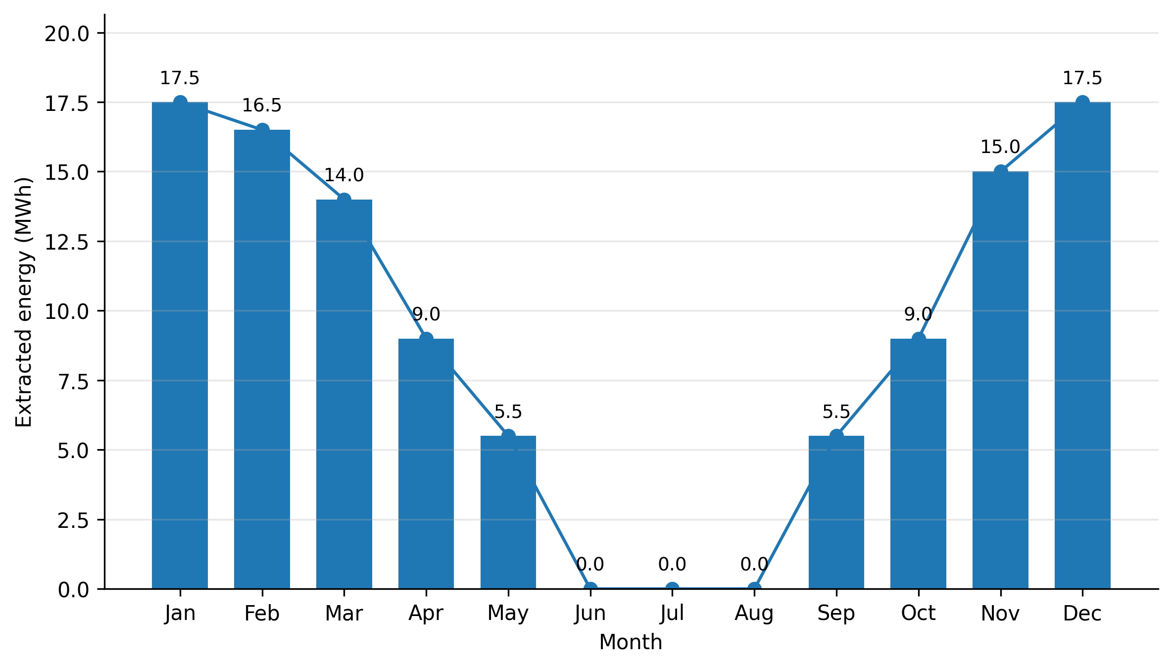
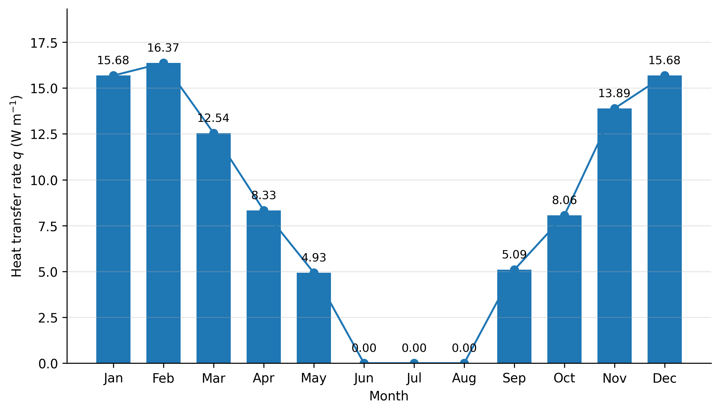
Figure 2: Annual source load profile repeatedly used in the simulations.. a — Extracted energy per month., b — Heat transfer rate per month of the considered system consisting of 25 BHEs with identical lengths \(L=100\)m and heat transfer rates.
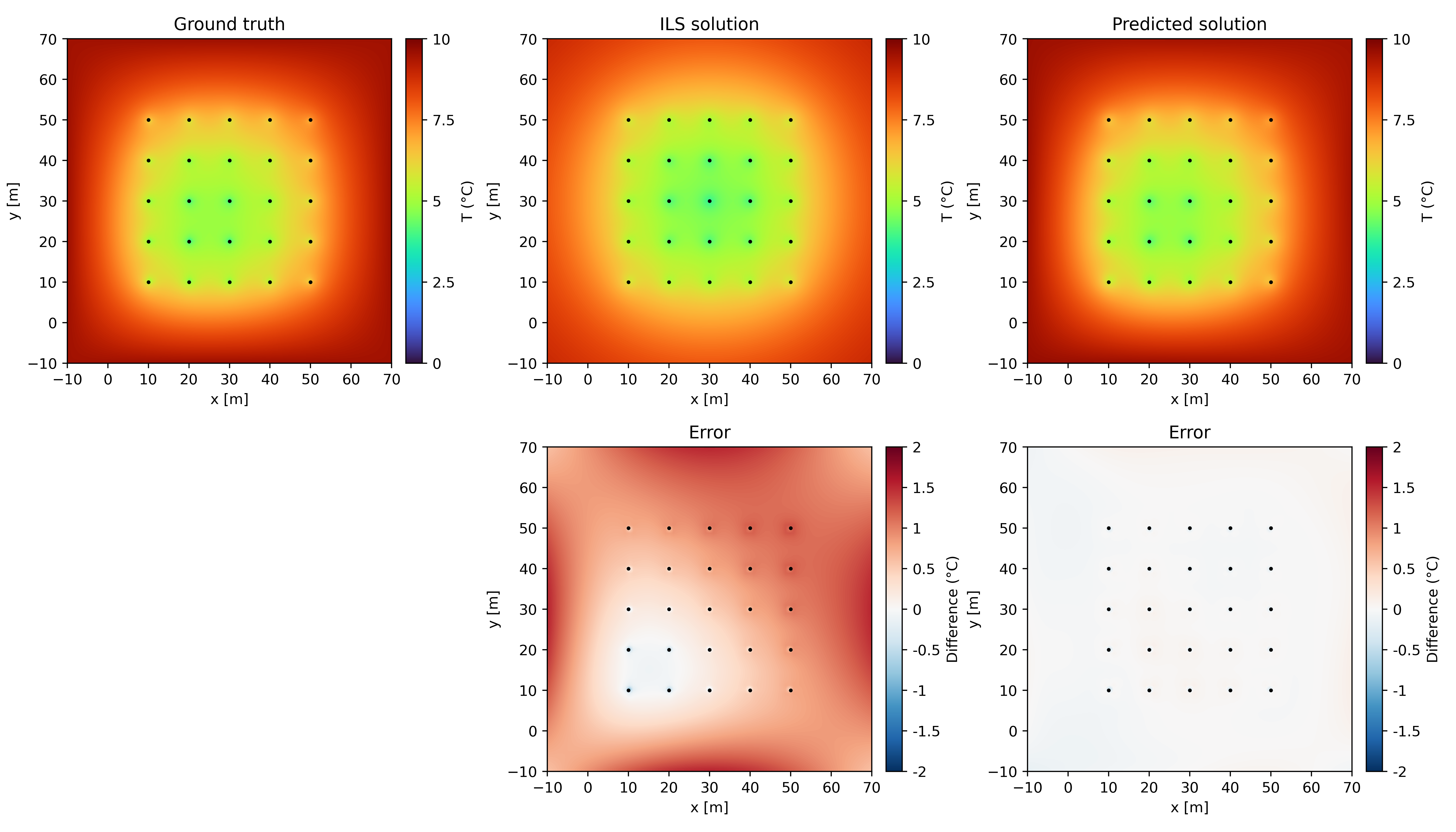
The compared distributions by numerical methods, analytical models and hybrid correctors are shown in Fig. 3 and Fig. 4, while the error metrics are summarized in Tables 3 and 4. For brevity, we only present the results for December of the 15th year and provide those for other selected time steps in the Appendix. As is shown, the ILS error exhibits a structured asymmetry along the conductivity gradient direction and significant mismatch near the boundary, and the corrected solution largely removes the bias and recovers the residual introduced by the soil heterogeneity.

| Month | Global ILS | Local ILS | Predicted solution | |||
|---|---|---|---|---|---|---|
| 2-3 (lr)4-5 (lr)6-7 | \(L^2\) | \(L^{\infty}\) | \(L^2\) | \(L^{\infty}\) | \(L^2\) | \(L^{\infty}\) |
| 60 | \(2.2994\mathrm{e}{-2}\) | \(1.2238\mathrm{e}{-1}\) | \(1.7270\mathrm{e}{-2}\) | \(5.1837\mathrm{e}{-2}\) | \(5.3270\mathrm{e}{-3}\) | \(5.5080\mathrm{e}{-2}\) |
| 180 | \(1.1436\mathrm{e}{-1}\) | \(1.5807\mathrm{e}{-1}\) | \(1.0582\mathrm{e}{-1}\) | \(1.6973\mathrm{e}{-1}\) | \(6.3225\mathrm{e}{-3}\) | \(5.7884\mathrm{e}{-2}\) |
| 360 | \(2.5428\mathrm{e}{-1}\) | \(2.8531\mathrm{e}{-1}\) | \(2.5348\mathrm{e}{-1}\) | \(3.1442\mathrm{e}{-1}\) | \(7.1412\mathrm{e}{-3}\) | \(5.3680\mathrm{e}{-2}\) |
2.5pt
| Month | Global ILS | Local ILS | Predicted solution | |||
|---|---|---|---|---|---|---|
| 2-3 (lr)4-5 (lr)6-7 | \(L^2\) | \(L^{\infty}\) | \(L^2\) | \(L^{\infty}\) | \(L^2\) | \(L^{\infty}\) |
| 60 | \(2.0424\mathrm{e}{-2}\) | \(1.1411\mathrm{e}{-1}\) | \(1.7429\mathrm{e}{-2}\) | \(5.0191\mathrm{e}{-2}\) | \(4.9878\mathrm{e}{-3}\) | \(5.5785\mathrm{e}{-2}\) |
| 180 | \(1.1324\mathrm{e}{-1}\) | \(1.5807\mathrm{e}{-1}\) | \(1.0956\mathrm{e}{-1}\) | \(1.6373\mathrm{e}{-1}\) | \(5.4639\mathrm{e}{-3}\) | \(5.9050\mathrm{e}{-2}\) |
| 360 | \(2.5934\mathrm{e}{-1}\) | \(2.8531\mathrm{e}{-1}\) | \(2.5968\mathrm{e}{-1}\) | \(2.9941\mathrm{e}{-1}\) | \(6.6568\mathrm{e}{-3}\) | \(5.6409\mathrm{e}{-2}\) |
3.0pt
4.0.0.2 Example 2.(FLS-based Model)
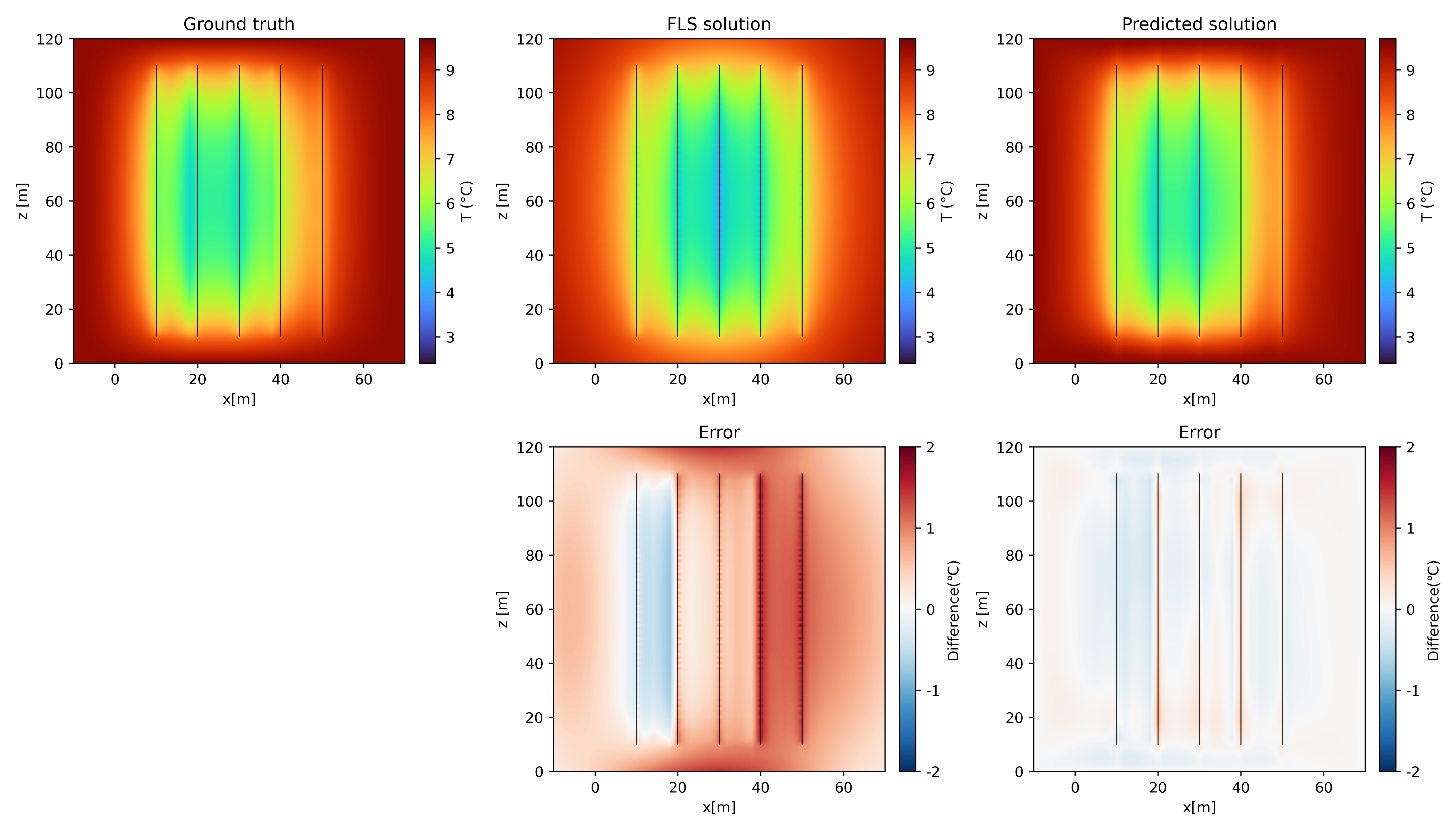
In this example, the same computational domain, simulation period, BHE arrangement and input sampling are applied as those of ILS-based model. Here, FLS models each BHE as a vertical line source with zero radius starting at depth \(D=10\)m and extending to \(D+L=110\)m. The vertical coordinates of training points are sampled from the source endpoint regions (\(z\in[4,16]\bigcup [104,116])\)m, the active source segment (\(z\in[10,110]\)m) and the complete vertical plane with probabilities \(\beta_0=0.45\), \(\beta_1=0.35\) and \(\beta_2=0.2\), respectively.
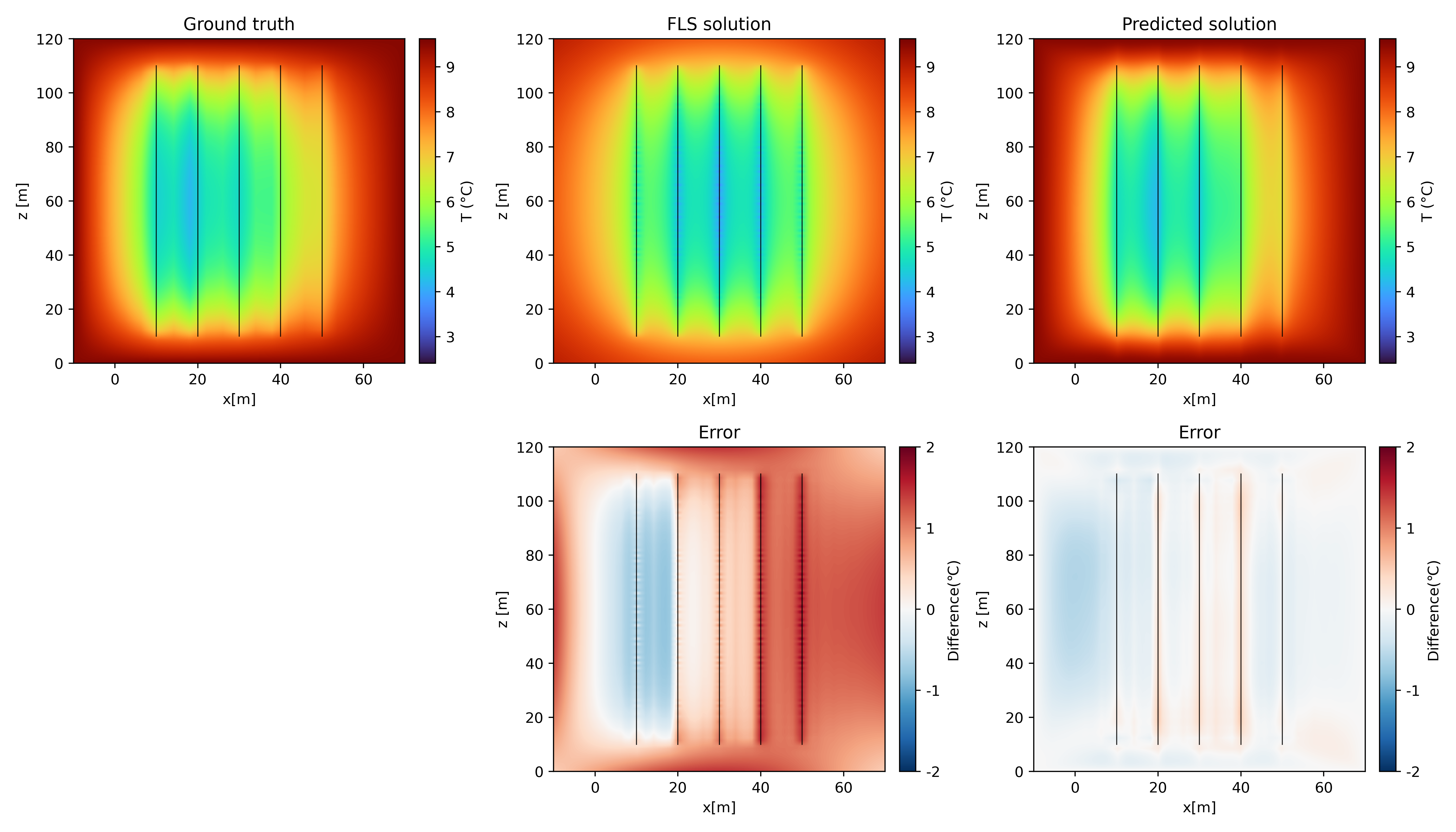
The results tested in December of the 15th year are presented in Figs. 5 and 6, where the temperature fields are visualized on the \(y=30\) and \(y=x\) cross sections for Scenario 1 and Scenario 2, respectively. And the relative error for all three tested time steps are reported in Tables 5 and 6.
| Month | Global FLS | Local FLS | Predicted solution | |||
|---|---|---|---|---|---|---|
| 2-3 (lr)4-5 (lr)6-7 | \(L^2\) | \(L^{\infty}\) | \(L^2\) | \(L^{\infty}\) | \(L^2\) | \(L^{\infty}\) |
| 60 | \(3.9753\mathrm{e}{-2}\) | \(1.1426\mathrm{e}{-1}\) | \(2.8918\mathrm{e}{-2}\) | \(1.0314\mathrm{e}{-1}\) | \(1.3647\mathrm{e}{-2}\) | \(6.5663\mathrm{e}{-2}\) |
| 180 | \(1.1527\mathrm{e}{-1}\) | \(2.0087\mathrm{e}{-1}\) | \(9.9794\mathrm{e}{-2}\) | \(1.5969\mathrm{e}{-1}\) | \(2.6352\mathrm{e}{-2}\) | \(6.2691\mathrm{e}{-2}\) |
| 360 | \(2.0594\mathrm{e}{-1}\) | \(3.0093\mathrm{e}{-1}\) | \(2.0303\mathrm{e}{-1}\) | \(2.7113\mathrm{e}{-1}\) | \(3.3584\mathrm{e}{-2}\) | \(8.4673\mathrm{e}{-2}\) |
3.0pt
| Month | Global FLS | Local FLS | Predicted solution | |||
|---|---|---|---|---|---|---|
| 2-3 (lr)4-5 (lr)6-7 | \(L^2\) | \(L^{\infty}\) | \(L^2\) | \(L^{\infty}\) | \(L^2\) | \(L^{\infty}\) |
| 60 | \(3.5310\mathrm{e}{-2}\) | \(1.3641\mathrm{e}{-1}\) | \(2.7753\mathrm{e}{-2}\) | \(1.1455\mathrm{e}{-1}\) | \(1.2180\mathrm{e}{-2}\) | \(6.6961\mathrm{e}{-2}\) |
| 180 | \(9.3774\mathrm{e}{-2}\) | \(2.1277\mathrm{e}{-1}\) | \(8.5121\mathrm{e}{-2}\) | \(1.6648\mathrm{e}{-1}\) | \(1.4805\mathrm{e}{-2}\) | \(6.0220\mathrm{e}{-2}\) |
| 360 | \(1.7720\mathrm{e}{-1}\) | \(3.1260\mathrm{e}{-1}\) | \(1.7586\mathrm{e}{-1}\) | \(2.6513\mathrm{e}{-1}\) | \(2.4955\mathrm{e}{-2}\) | \(8.7812\mathrm{e}{-2}\) |
3.0pt
4.0.0.3 Example 3.(MFLS-based Model)
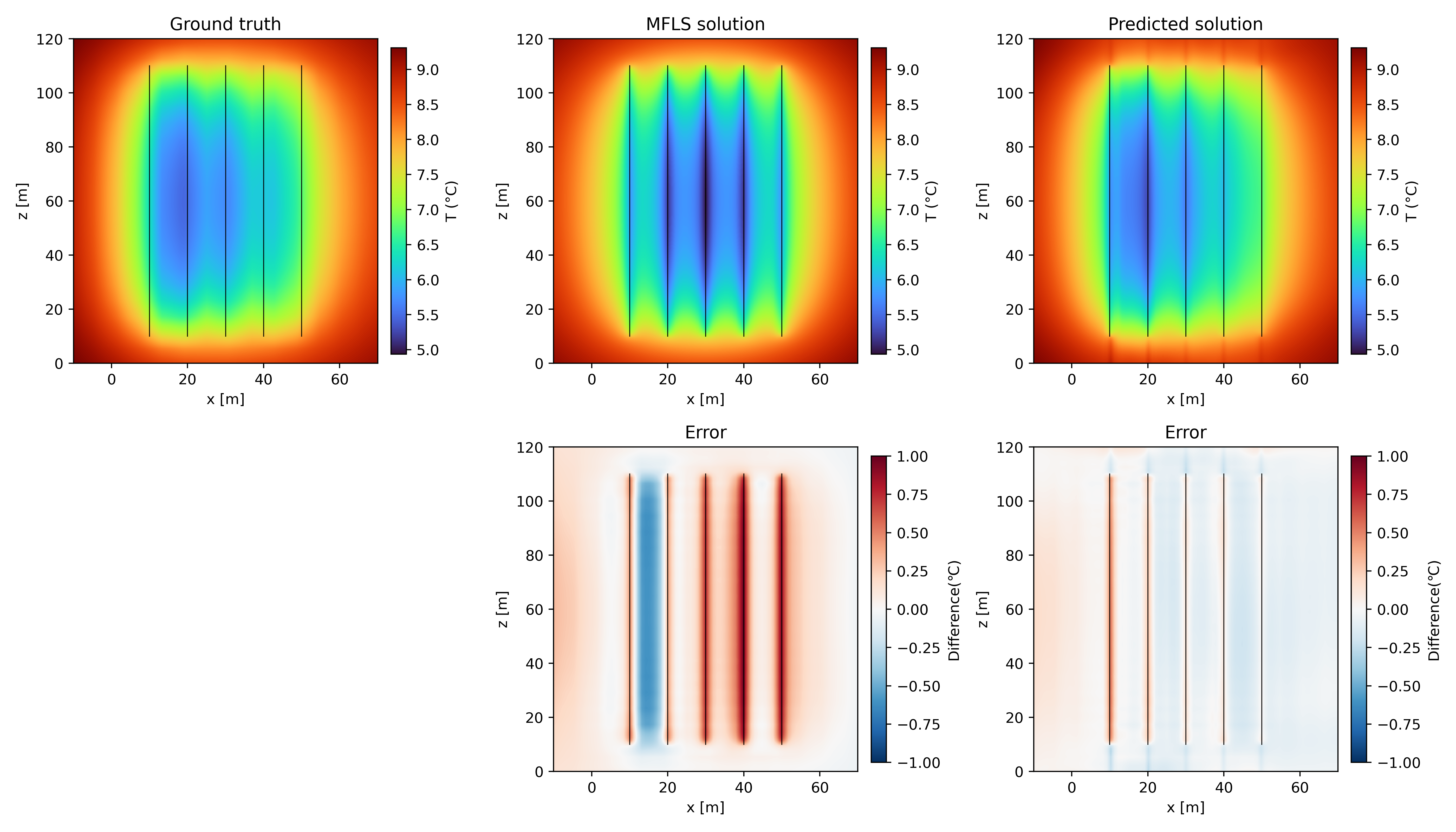
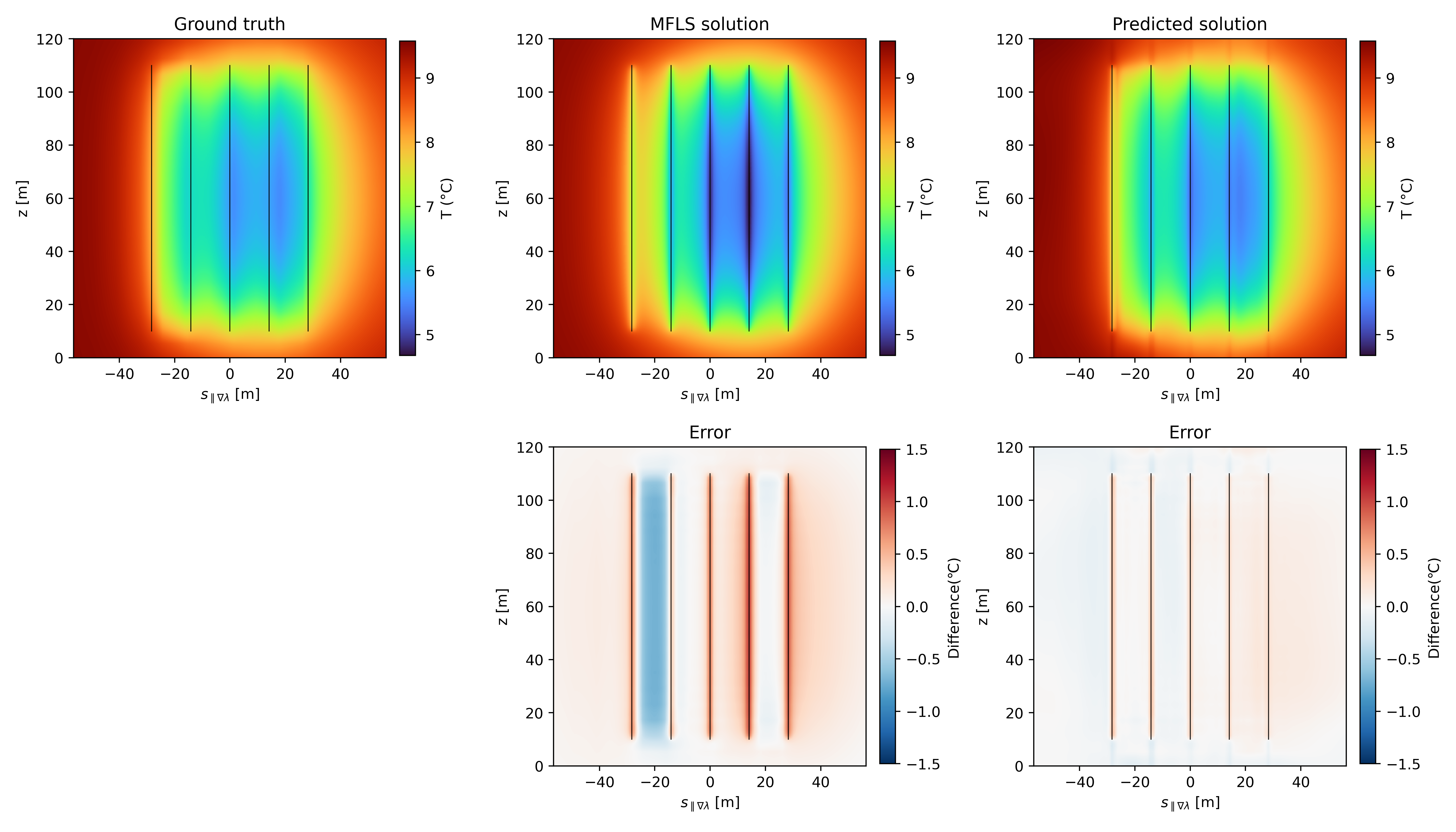
We employ the same computational setup and training configuration as FLS-based model to this case. We choose \(\mathrm{\mathbf{v}}=\left(0,2,0\right)\)m/year for training and inference in this test. To examine the effects of conductivity and groundwater advection, we evaluate the predicted temperature fields on two representative vertical sections which are aligned with the conductivity gradient and groundwater flow direction respectively for both scenarios. The simulation results for Scenario 1 are exhibited in Fig. 7 and Fig. 8 and Scenario 2 in Fig. 9 and Fig. 10. The corresponding horizontal slices at \(z=60\) are provided in Appendix.
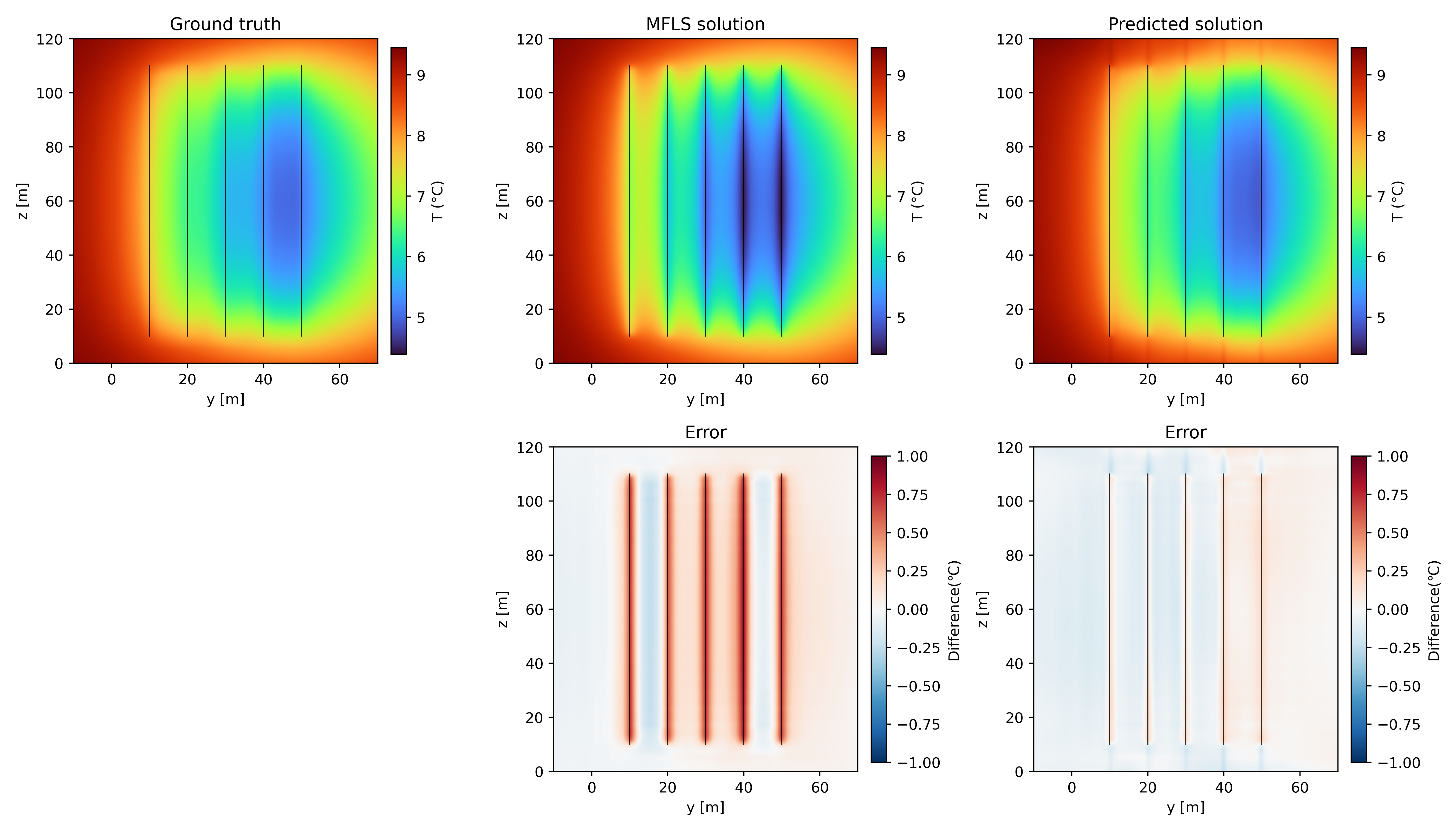
Tables 7 and 8 show the comparison between the accuracy performance of global MFLS solution, local MFLS solution and predicted approximation on the cross sections \(y=30\), \(y=x\) for Scenarios 1 and 2, respectively.

| Month | Global MFLS | Local MFLS | Predicted solution | |||
|---|---|---|---|---|---|---|
| 2-3 (lr)4-5 (lr)6-7 | \(L^2\) | \(L^{\infty}\) | \(L^2\) | \(L^{\infty}\) | \(L^2\) | \(L^{\infty}\) |
| 60 | \(3.1835\mathrm{e}{-2}\) | \(9.5800\mathrm{e}{-2}\) | \(3.3631\mathrm{e}{-2}\) | \(1.3052\mathrm{e}{-1}\) | \(1.2883\mathrm{e}{-2}\) | \(6.5947\mathrm{e}{-2}\) |
| 180 | \(3.8989\mathrm{e}{-2}\) | \(1.0668\mathrm{e}{-1}\) | \(3.8217\mathrm{e}{-2}\) | \(1.3185\mathrm{e}{-1}\) | \(1.4186\mathrm{e}{-2}\) | \(5.8802\mathrm{e}{-2}\) |
| 360 | \(3.9346\mathrm{e}{-2}\) | \(1.0401\mathrm{e}{-1}\) | \(3.7546\mathrm{e}{-2}\) | \(1.2719\mathrm{e}{-1}\) | \(1.9900\mathrm{e}{-2}\) | \(5.1020\mathrm{e}{-2}\) |
3.0pt
| Month | Global MFLS | Local MFLS | Predicted solution | |||
|---|---|---|---|---|---|---|
| 2-3 (lr)4-5 (lr)6-7 | \(L^2\) | \(L^{\infty}\) | \(L^2\) | \(L^{\infty}\) | \(L^2\) | \(L^{\infty}\) |
| 60 | \(3.0866\mathrm{e}{-2}\) | \(9.4315\mathrm{e}{-2}\) | \(3.2402\mathrm{e}{-2}\) | \(1.3027\mathrm{e}{-1}\) | \(1.0262\mathrm{e}{-2}\) | \(5.5186\mathrm{e}{-2}\) |
| 180 | \(3.9475\mathrm{e}{-2}\) | \(1.0962\mathrm{e}{-1}\) | \(3.8389\mathrm{e}{-2}\) | \(1.2948\mathrm{e}{-1}\) | \(1.3497\mathrm{e}{-2}\) | \(5.3051\mathrm{e}{-2}\) |
| 360 | \(4.2862\mathrm{e}{-2}\) | \(1.0943\mathrm{e}{-1}\) | \(4.0260\mathrm{e}{-2}\) | \(1.2774\mathrm{e}{-1}\) | \(1.5536\mathrm{e}{-2}\) | \(5.2131\mathrm{e}{-2}\) |
3.0pt
5 Conclusion↩︎
In this paper, we develop a parametric hybrid-PINN method, based on ILS, FLS and MFLS analytical models, for thermal simulation of borehole heat exchangers, i.e. singular line sources, in heterogeneous subsurface. By decomposing the global soil temperature distribution into an analytical baseline and a learned correction, we remove the challenge for the network to accurately capture the singularity and avoid the need to approach the delta function using traditional regularization tools. For the ILS and FLS based models, the goal of the correction component is to characterize both mismatches induced by formation properties and boundary conditions on account of the idealized assumptions of the analytical models on the soil homogeneity and domain boundary. The MFLS-based model mainly accounts for the former under an open boundary setting.
We propose a parametric physics-informed neural network to approximate the temperature correction governed by the correction equation and initial condition, with Dirichlet boundary treatment enforced for conduction-dominated cases. To inform the network the relative position of any input coordinate with respect to the borehole source and boundary interfaces, we include location indicator functions as additional feature inputs to the network, endowing it with capability of learning local and global behaviors simultaneously. In addition, we adopt a source-centered sampling strategy for generating physics collocation and data points to handle the correction distribution imbalance over the space and time scales. The physics-informed and data-supervised loss function is constructed via evaluating all the sampled gradient conductivity conditions on these adaptively placed training points. The inference efficiency is attained through applying the superposition principles to the trained universal corrector. We perform numerical experiments to show the effectiveness of the proposed method on top of all ILS, FLS and MFLS models in a multi-BHE domain over a long simulation period. As demonstrated in presented results, the tested examples can be solved with acceptable accuracy by the parametric hybrid-PINN universal corrector with moderate number of supervised data samples. Future research will extend to providing more comprehensive models for BHE simulation by coupling the heat transport inside the borehole to soil temperature response. The fast and differentiable nature of the learned corrector also makes it promising for PDE-constrained optimization, including borehole layout design, installation length, load profile planning and long-term operational scheduling. Another future development is to explore frameworks which can solve more complex soil property fields and include a broader set of design and operation parameters. As the parametric space becomes higher-dimensional, more expressive learning architectures including neural operators, encoder-decoder structures and generative deep learning models, may be required to construct scalable surrogate models. Incorporating these directions in future work will further improve the proposed methodology, enabling it to serve as a more extensive tool for the efficient simulation and optimization of geothermal energy systems.
Conflict of Interest↩︎
The authors declare no conflicts of interest.
Acknowledgement↩︎
The work presented in this paper was supported by the German Federal Ministry of Economics and Climate Protection (BMWK) within the scope of the research project OptiGeoS (01256700/1).
Appendix↩︎
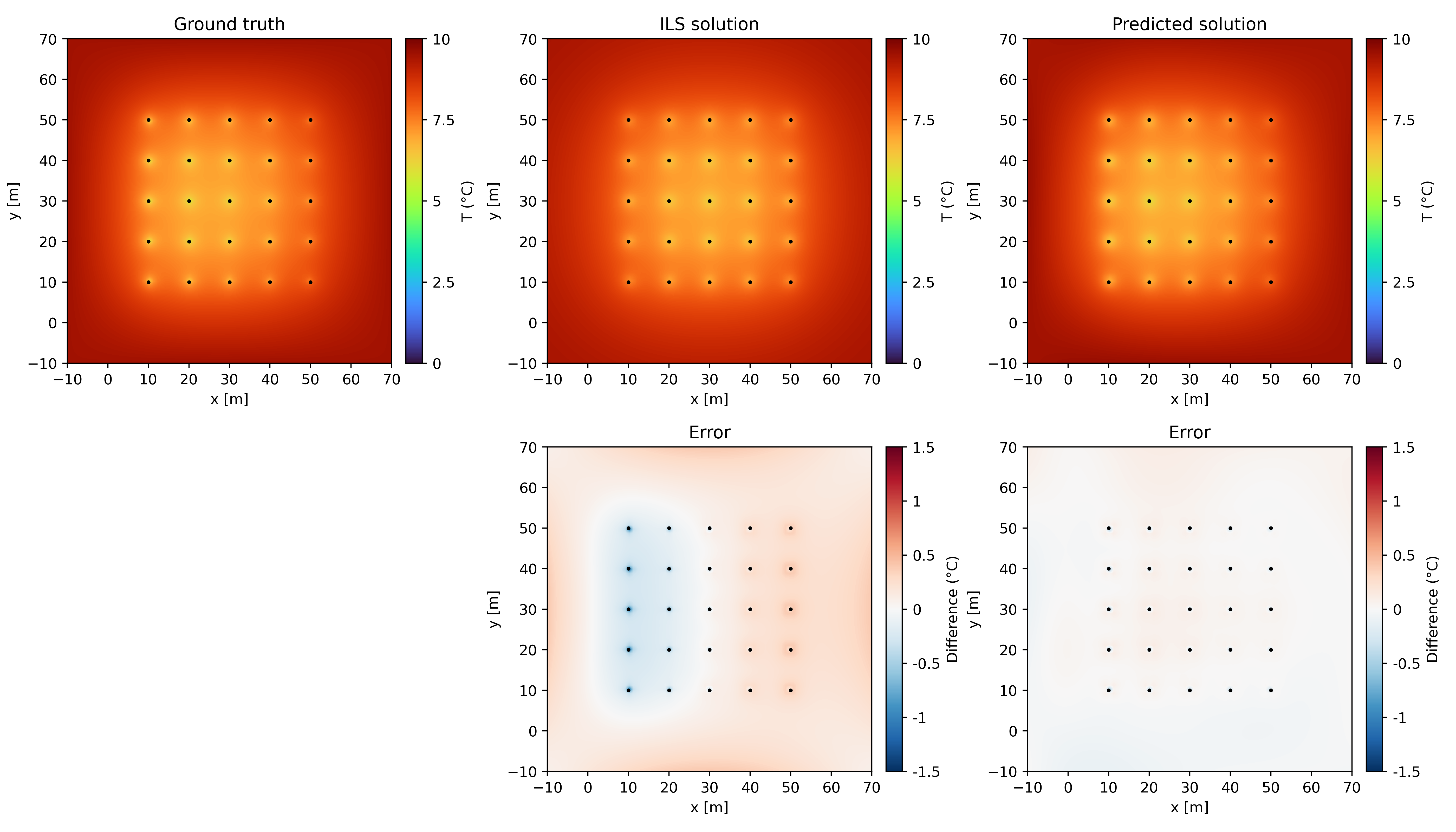
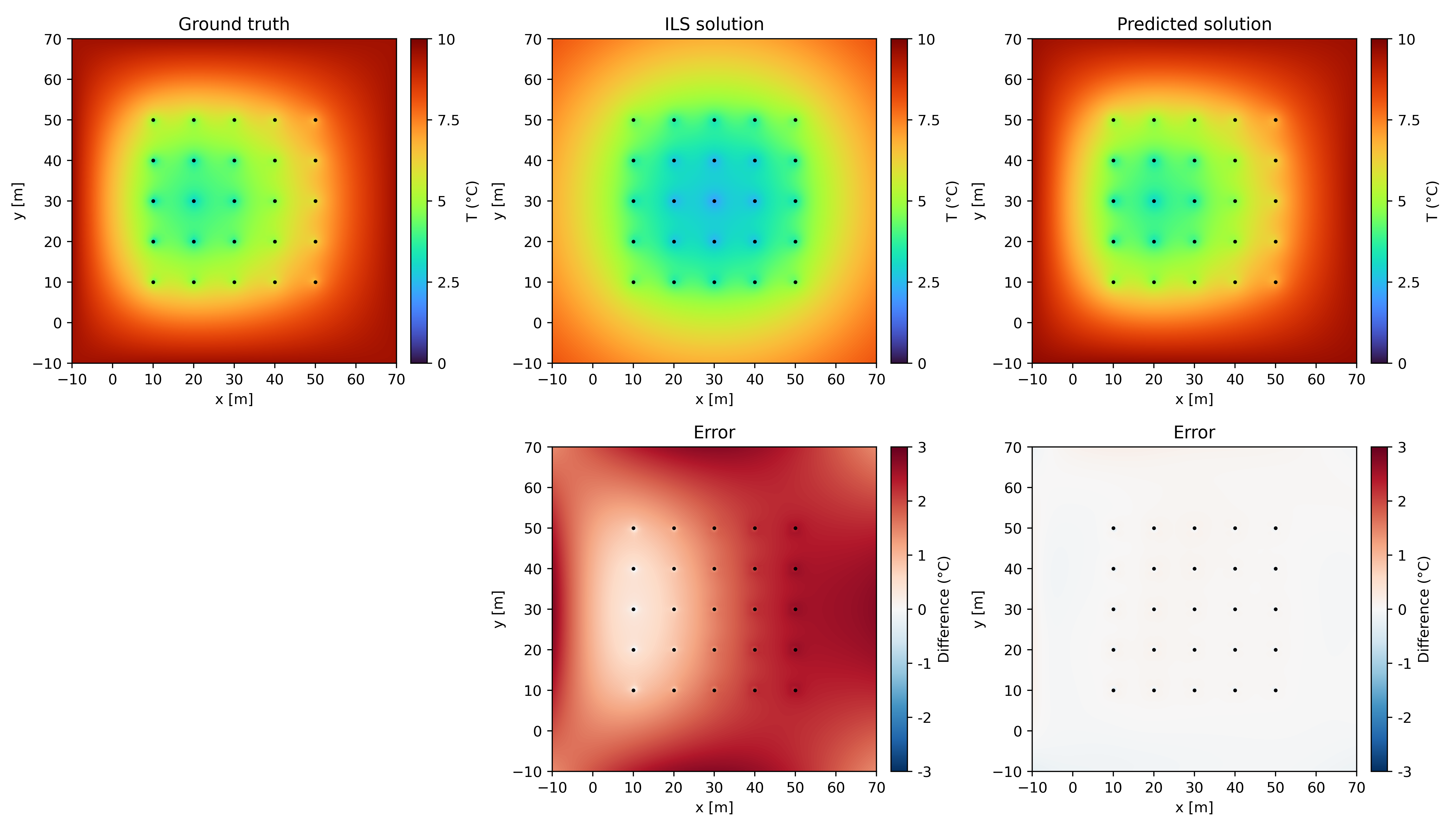
Figure 11: Temperature distributions for Scenario 1, derived from the finite difference solver (Ground truth, \(h=1\)m), ILS analytical formula (ILS solution) and hybrid-PINN corrector (Predicted solution) and the difference distributions of ILS solution and predicted solution with respect to the ground truth.. a — December of the \(5\)th simulated year., b — December of the \(30\)th simulated year.
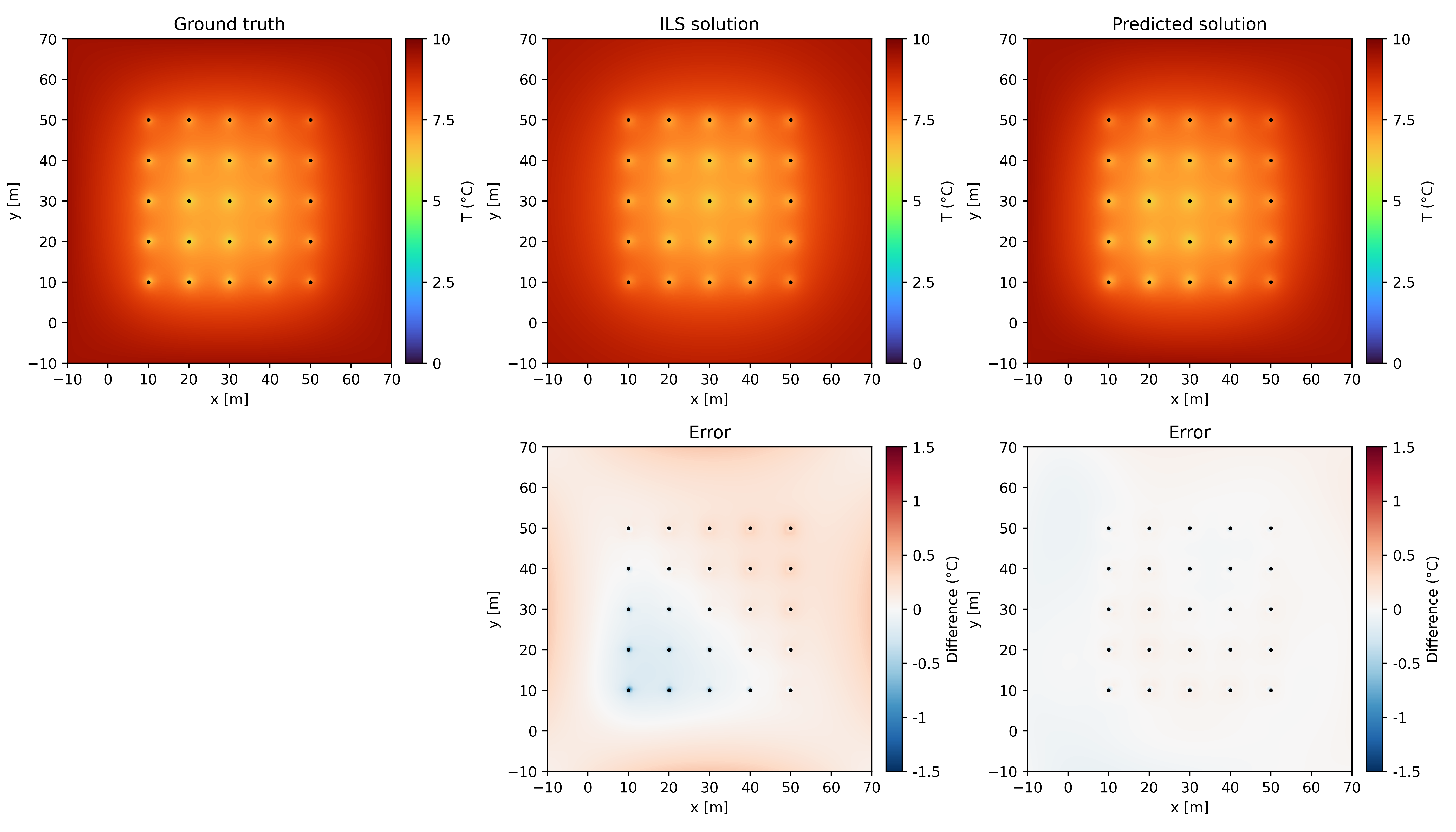
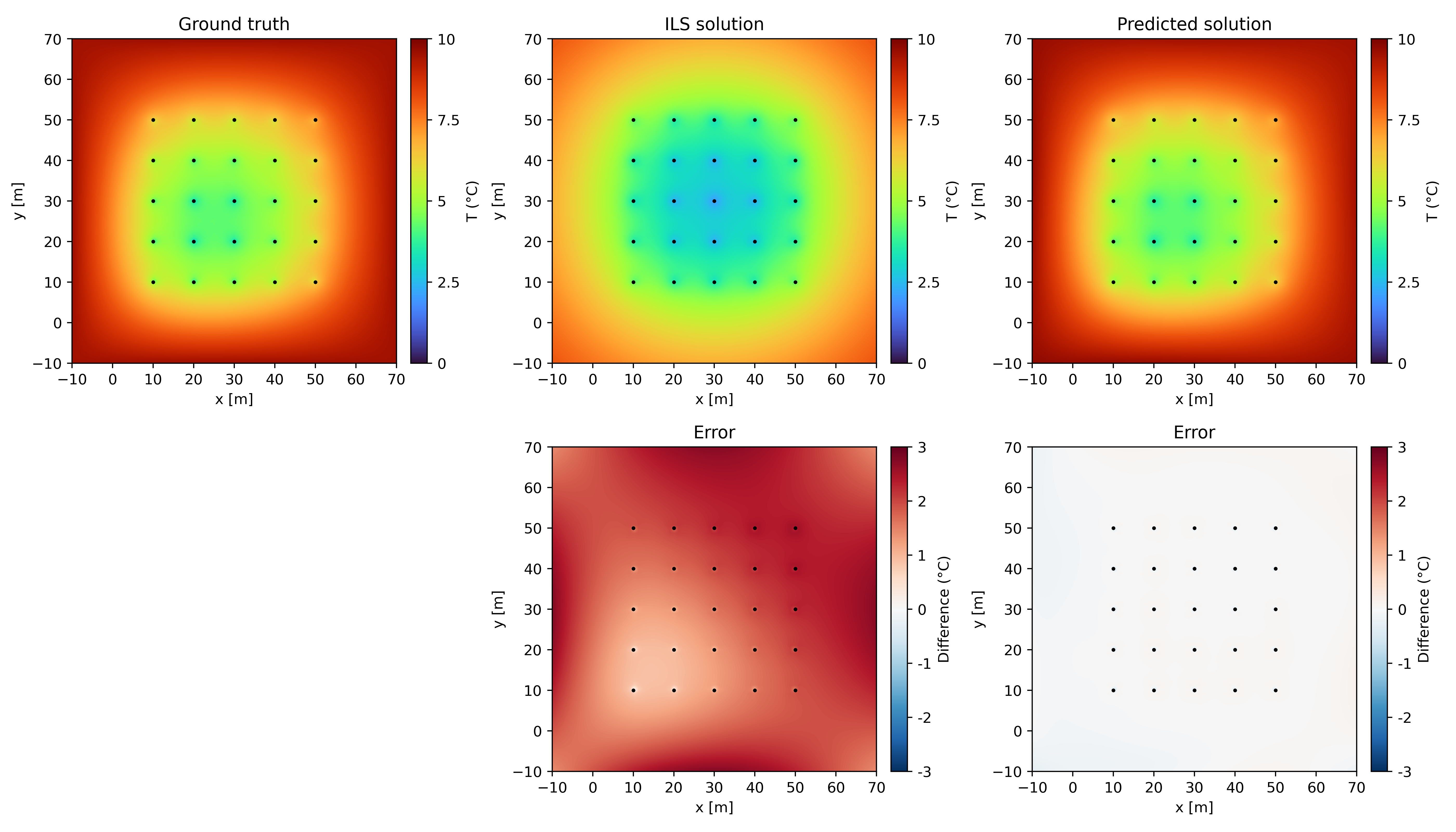
Figure 12: Temperature distributions for Scenario 2, derived from the finite difference solver (Ground truth, \(h=1\)m), ILS analytical formula (ILS solution) and hybrid-PINN corrector (Predicted solution) and the difference distributions of ILS solution and predicted solution with respect to the ground truth.. a — December of the \(5\)th simulated year., b — December of the \(30\)th simulated year.
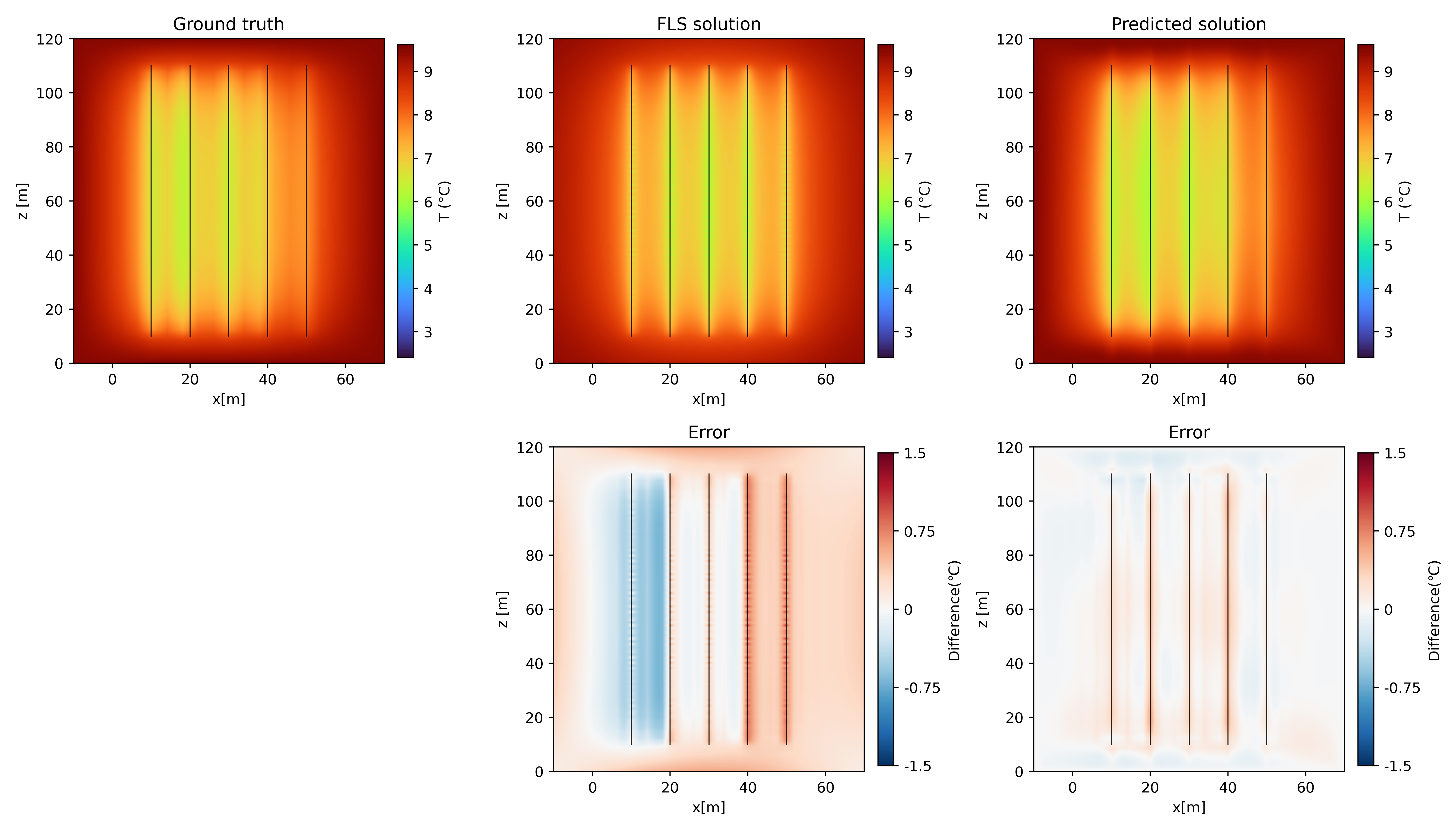
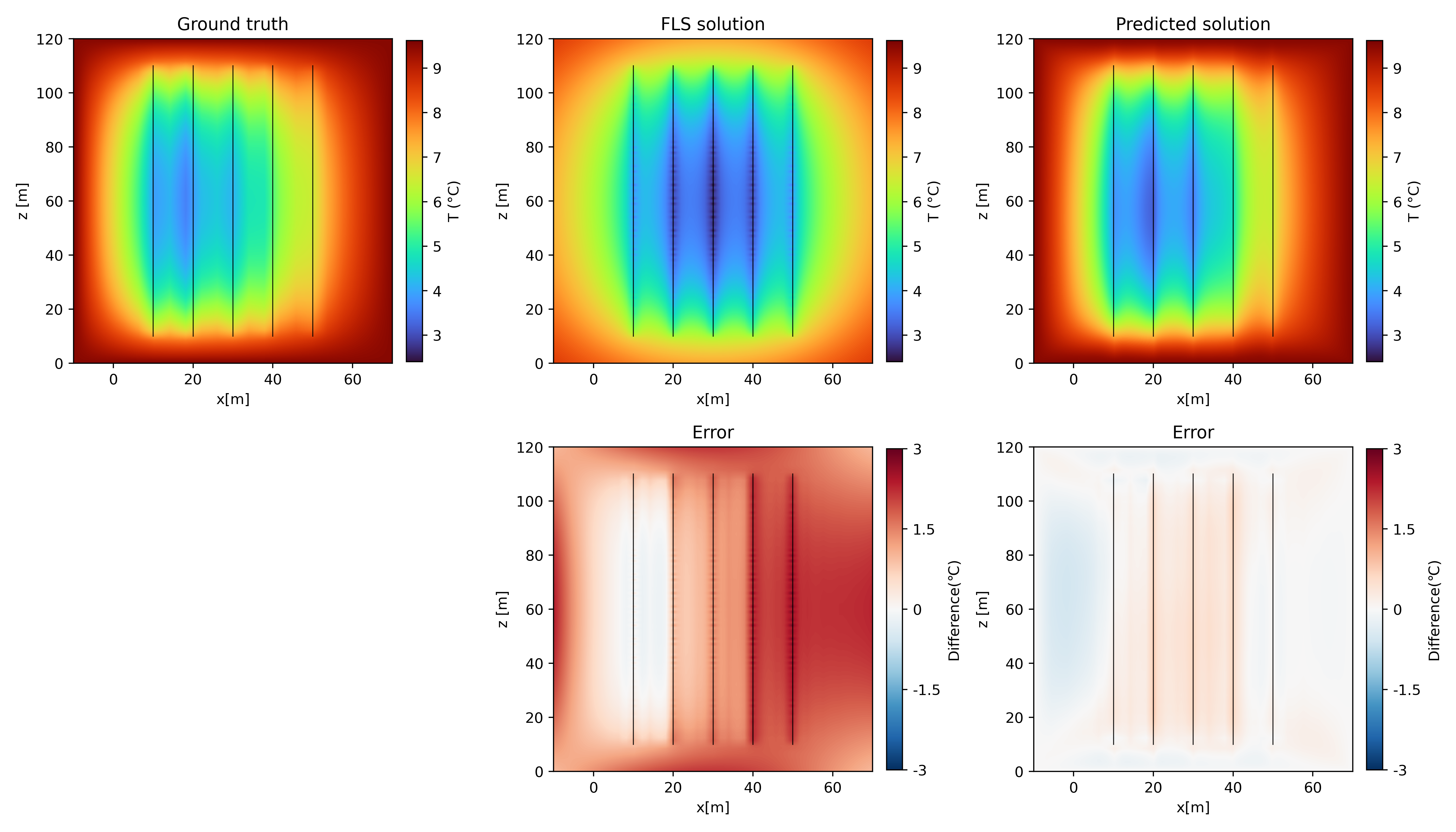
Figure 13: Temperature distributions on the vertical cross section \(y=30\) for Scenario 1, derived from the finite difference solver (Ground truth, \(h=1\)m), FLS analytical formula (FLS solution) and hybrid-PINN corrector (Predicted solution) and the difference distributions of FLS solution and predicted solution with respect to the ground truth on the same cross section.. a — December of the \(5\)th simulated year., b — December of the \(30\)th simulated year.
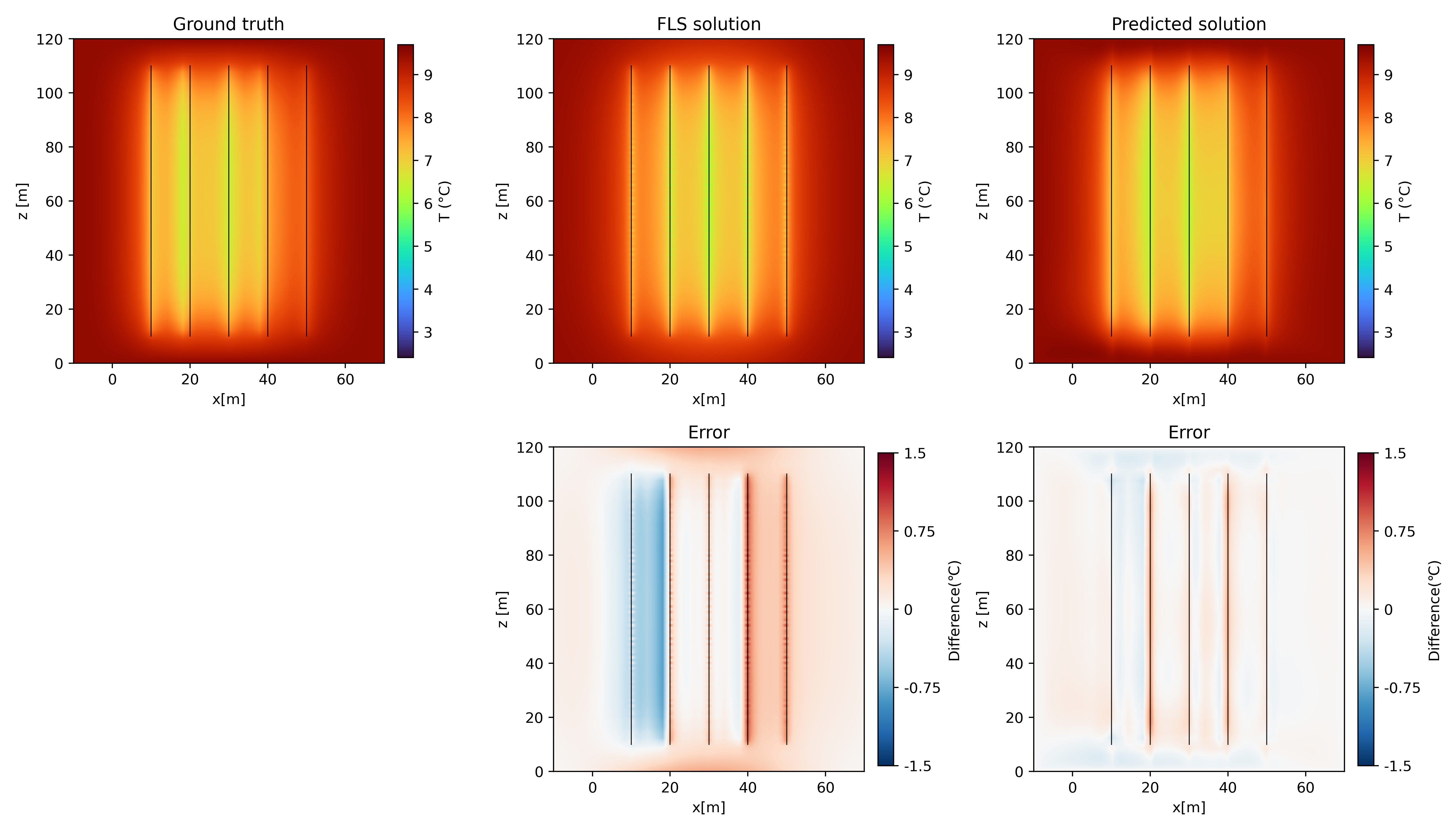

Figure 14: Temperature distributions on the vertical section \(y=x\) for Scenario 2, derived from the finite difference solver (Ground truth, \(h=1\)m), FLS analytical formula (FLS solution) and hybrid-PINN corrector (Predicted solution) and the difference distributions of FLS solution and predicted solution with respect to the ground truth on the same cross section. The horizontal coordinate is labeled by the projection onto the \(x\) axis.. a — December of the \(5\)th simulated year., b — December of the \(30\)th simulated year.
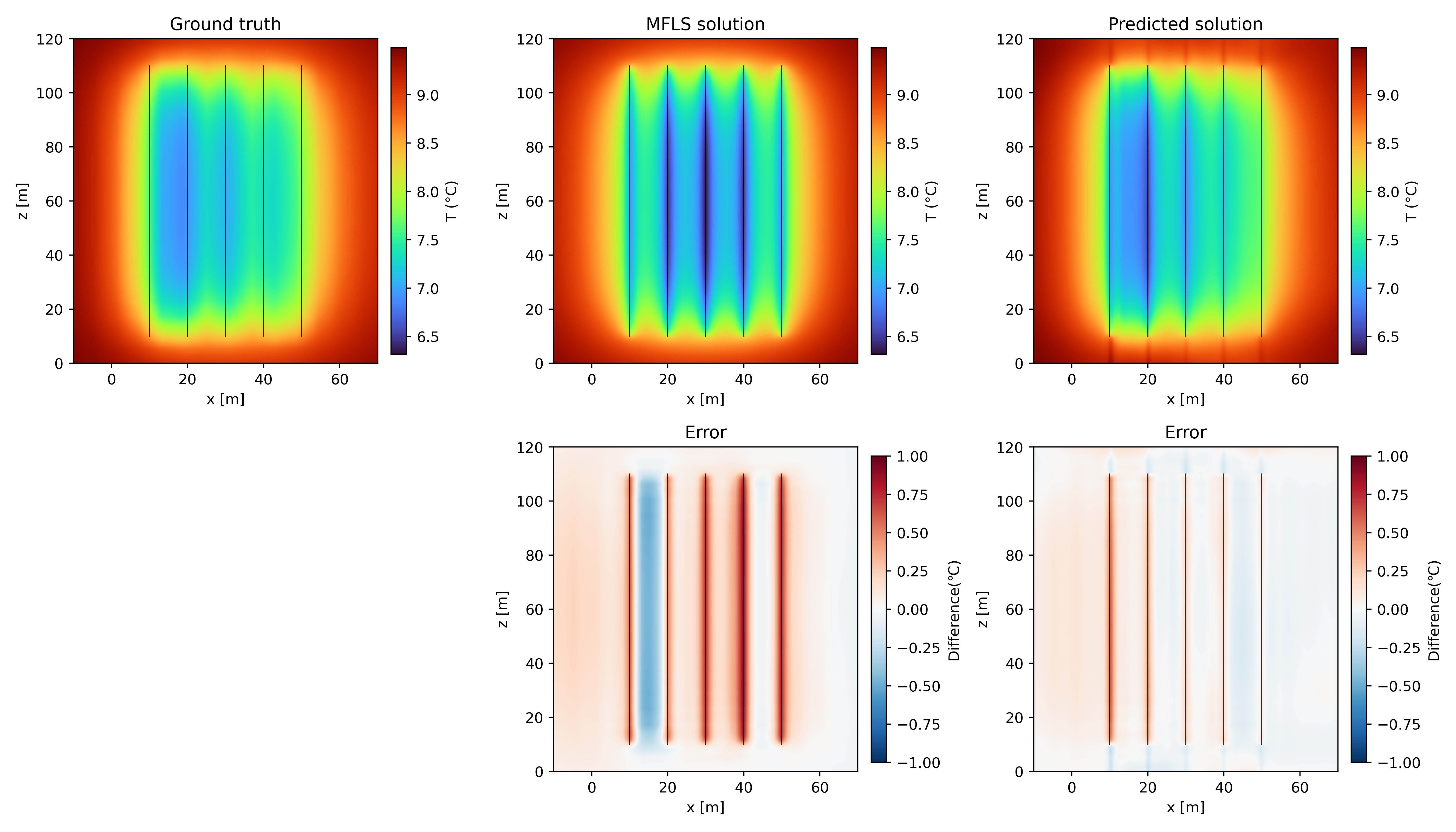
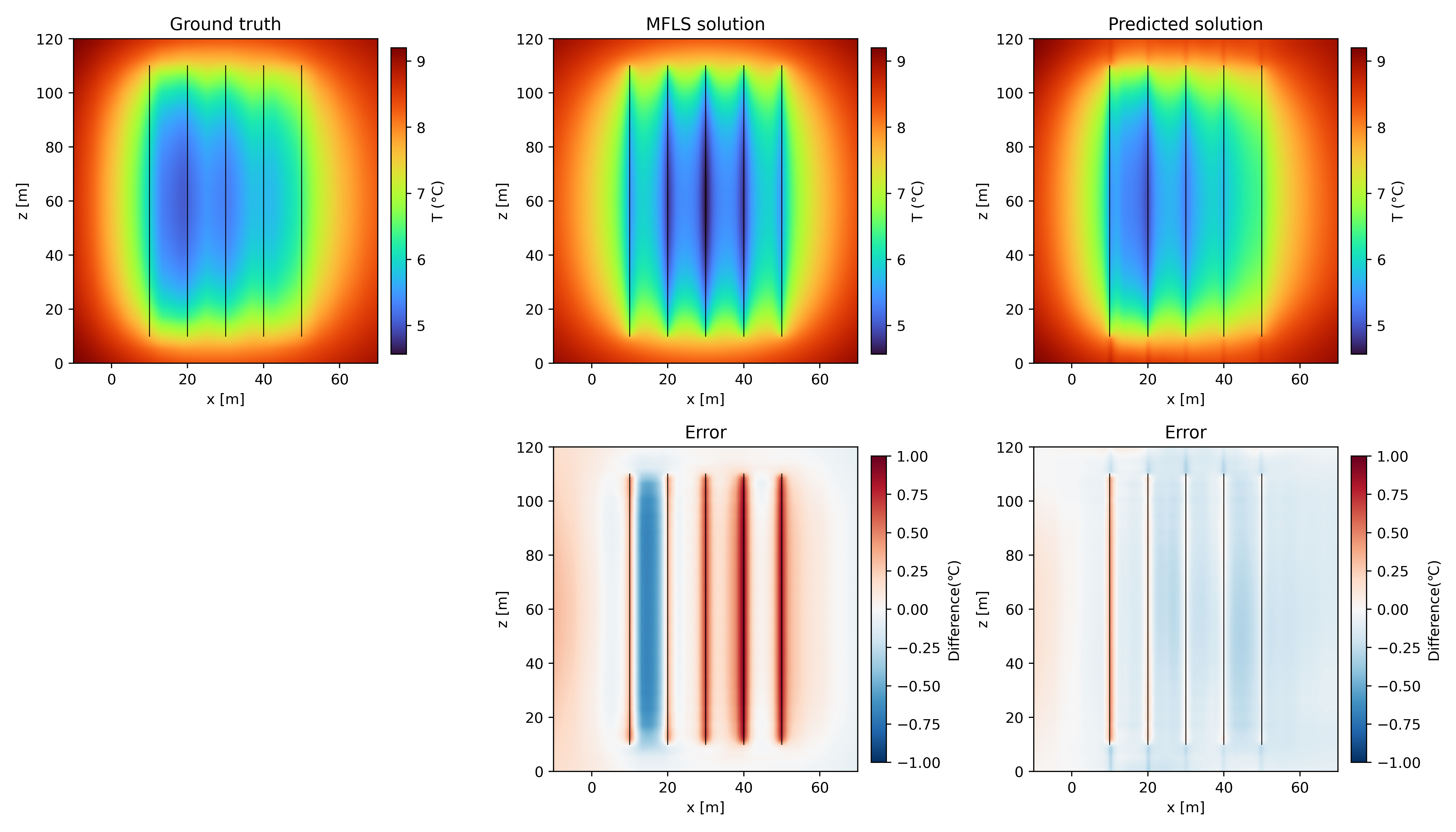
Figure 15: Temperature distributions on the vertical cross section \(y=30\) for Scenario 1, derived from the finite difference solver (Ground truth, \(h=1\)m), MFLS analytical formula (MFLS solution) and hybrid-PINN corrector (Predicted solution) and the difference distributions of MFLS solution and predicted solution with respect to the ground truth on the same cross section.. a — December of the \(5\)th simulated year., b — December of the \(30\)th simulated year.
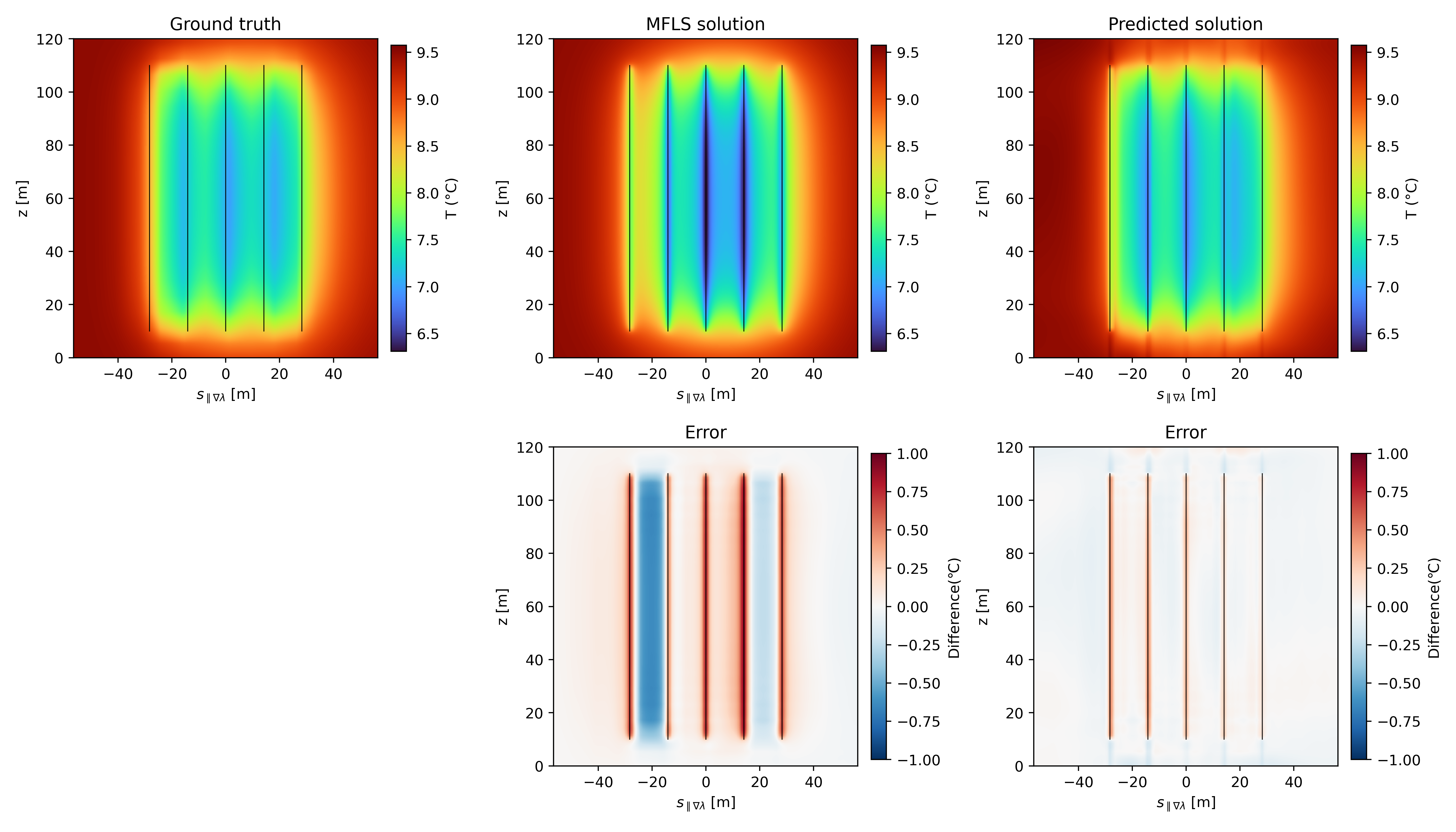
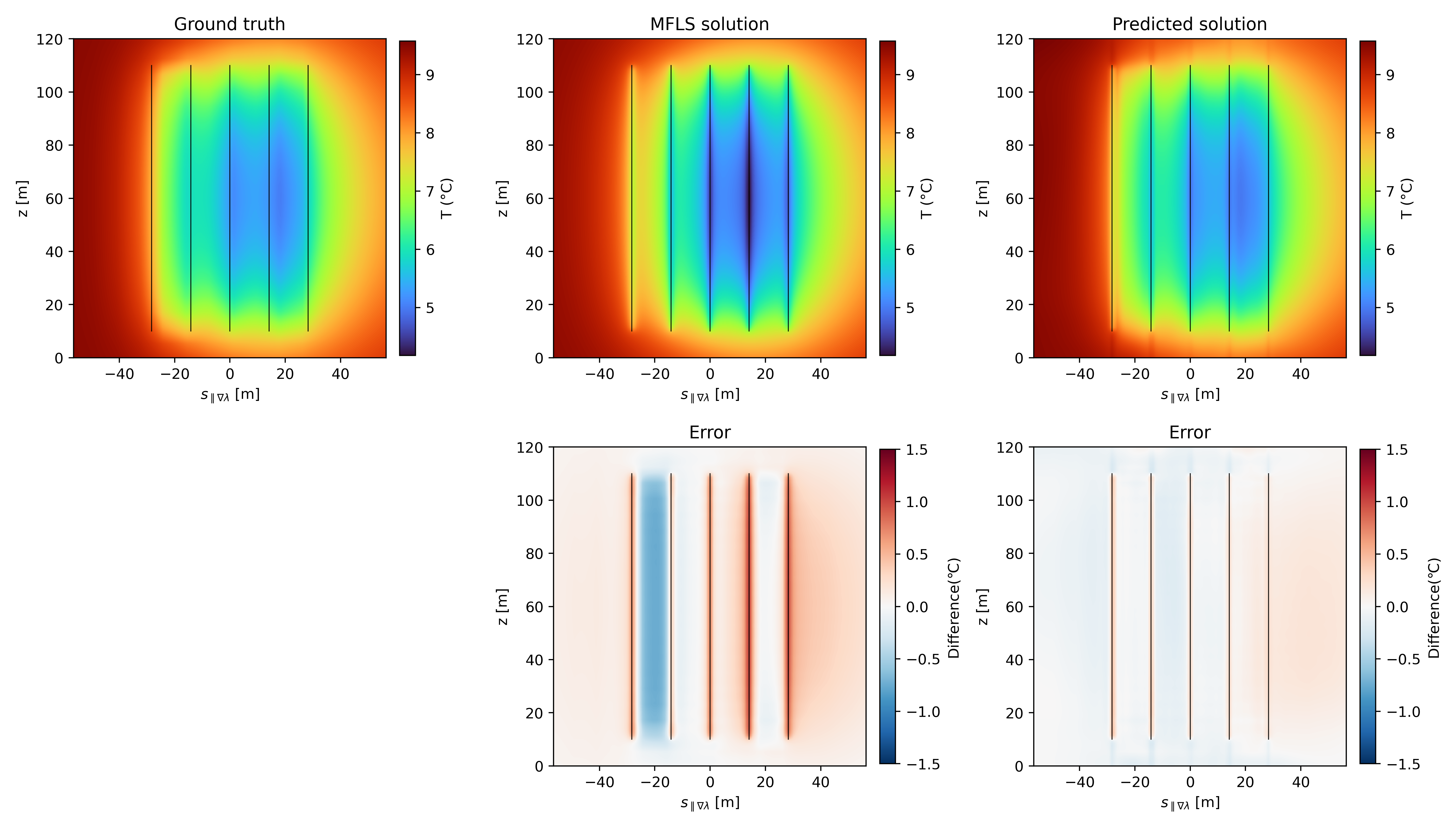
Figure 16: Temperature distributions on the vertical section \(y=x\) for Scenario 2, derived from the finite difference solver (Ground truth, \(h=1\)m), MFLS analytical formula (MFLS solution) and hybrid-PINN corrector (Predicted solution) and the difference distributions of MFLS solution and predicted solution with respect to the ground truth on the same cross section. The horizontal coordinate is labeled by the projection onto the \(x\) axis.. a — December of the \(5\)th simulated year., b — December of the \(30\)th simulated year.
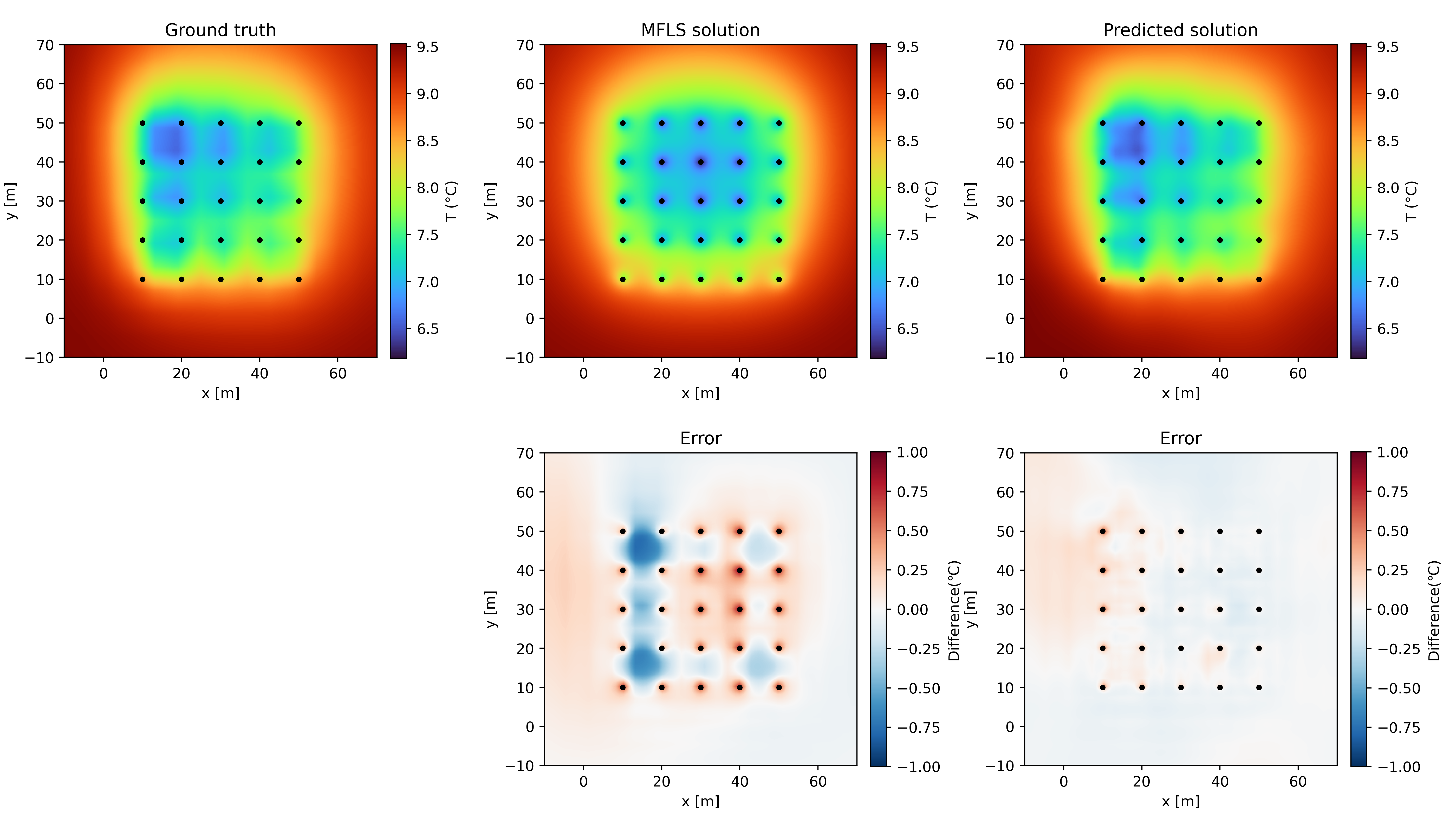
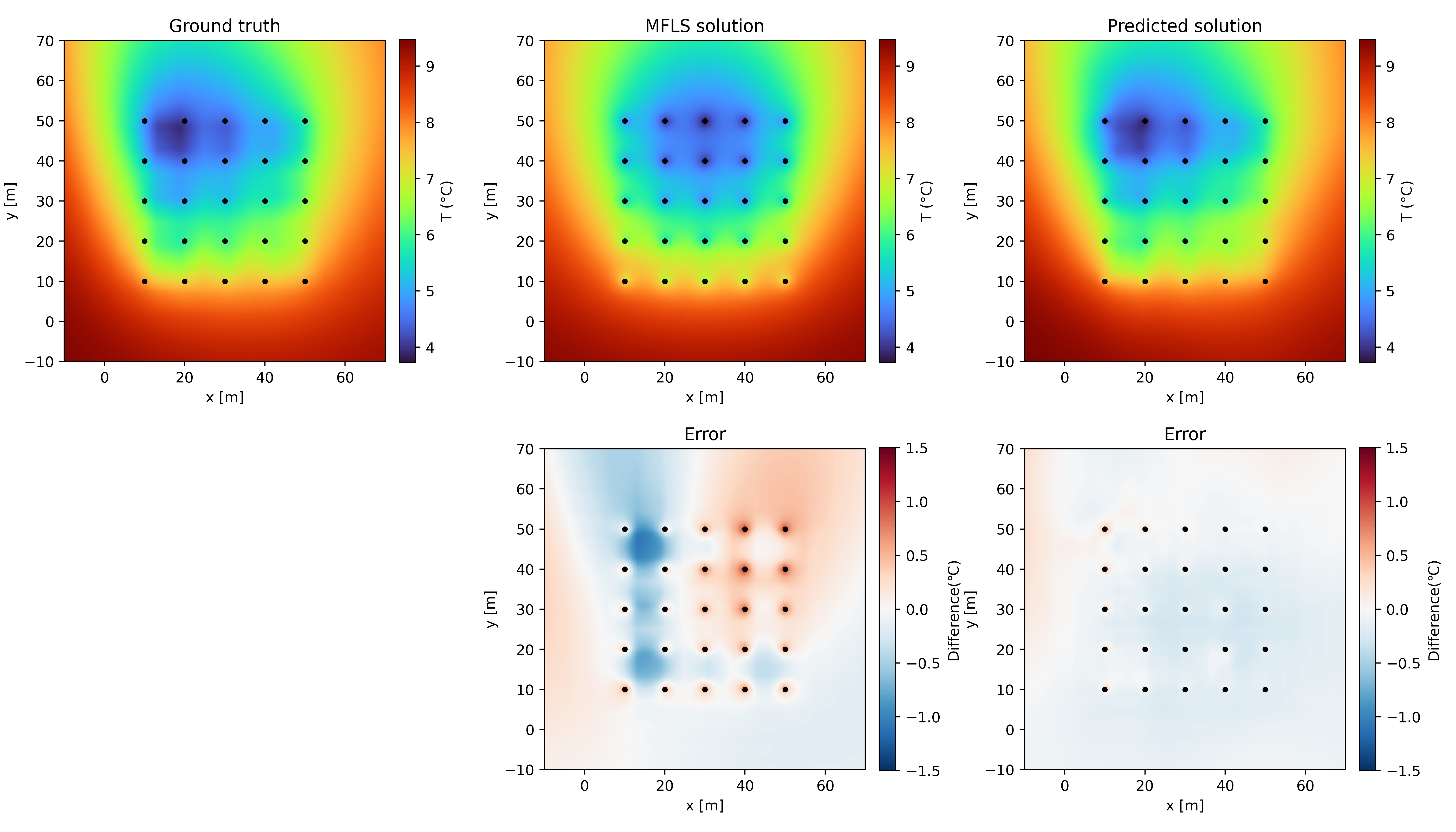
Figure 17: Temperature distributions on the horizontal section \(z=60\) for Scenario 1, derived from the finite difference solver (Ground truth, \(h=1\)m), MFLS analytical formula (MFLS solution) and hybrid-PINN corrector (Predicted solution) and the difference distributions of MFLS solution and predicted solution with respect to the ground truth on the same cross section.. a — December of the \(5\)th simulated year., b — December of the \(30\)th simulated year.
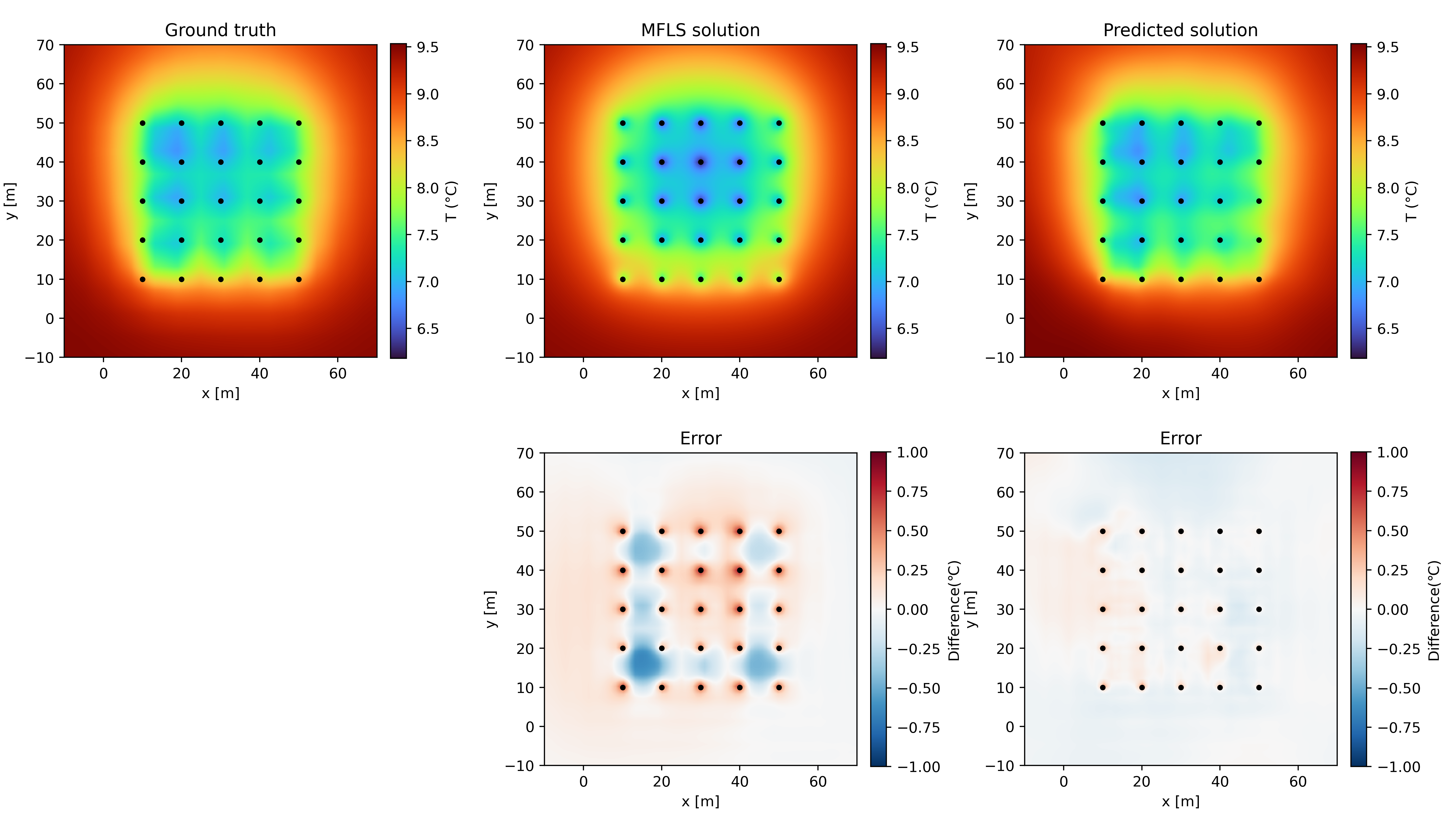
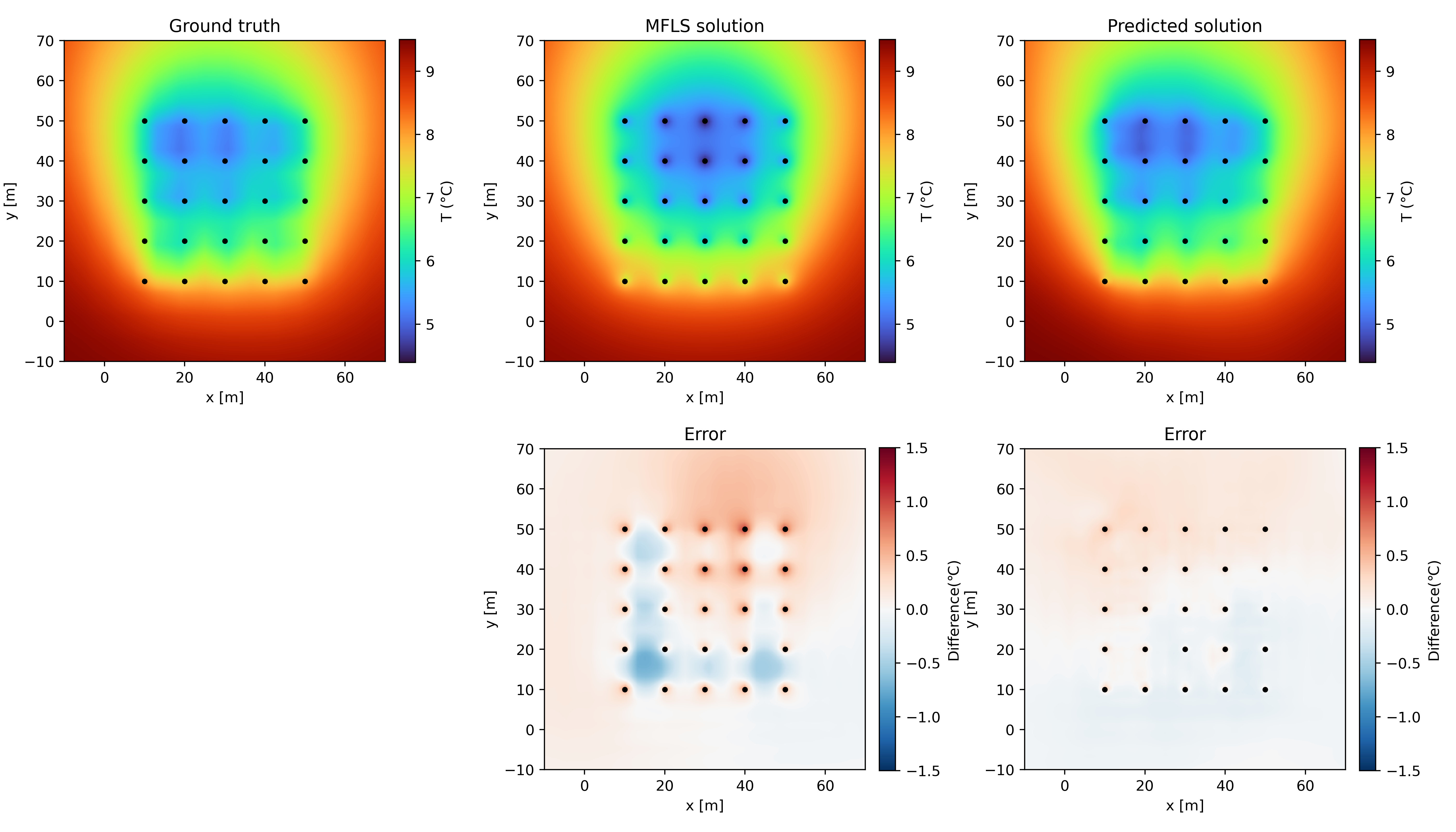
Figure 18: Temperature distributions on the horizontal section \(z=60\) for Scenario 2, derived from the finite difference solver (Ground truth, \(h=1\)m), MFLS analytical formula (MFLS solution) and hybrid-PINN corrector (Predicted solution) and the difference distributions of MFLS solution and predicted solution with respect to the ground truth on the same cross section.. a — December of the \(5\)th simulated year., b — December of the \(30\)th simulated year.
References↩︎
Corresponding author. Email: smajil.halilovic@tum.de↩︎