Contour-count indicator fields for visible pole clusters in meromorphic continuation
July 14, 2026
1 Introduction↩︎
Numerical analytic continuation is a classical problem in mathematical analysis, with important applications in scientific computing and engineering [1]. Its main difficulty is severe ill-conditioning: small perturbations in the input data may be strongly amplified after continuation, so direct numerical continuation is unstable without additional a priori information [2]. Substantial work has therefore been devoted to both the theoretical and computational stabilization of analytic continuation, including bounded continuation, conformal-mapping approaches, regularization methods, rational approximation, and fast Fourier based procedures [3]–[10]. Much of this literature concerns the stable continuation or approximation of holomorphic functions, or the reconstruction of analytic objects under prescribed regularity, boundedness, or rational-approximation assumptions. In contrast, the present paper focuses on a pole-oriented form of meromorphic continuation: rather than attempting direct pointwise extrapolation, we seek stable information about exterior poles that obstruct holomorphic continuation.
The pole-recovery viewpoint goes back at least to Miller’s stabilized numerical analytic prolongation with poles [6]. Miller formulated meromorphic continuation as a stabilized inverse problem and introduced the SNAPP algorithm, which seeks a rational approximant with the minimum number of poles compatible with the data and a prescribed global bound. This work already identifies pole recovery as a natural stabilized output of meromorphic continuation. More recently, Derevianko [11] developed a different Fourier-domain approach for recovering rational functions from their Fourier coefficients. By exploiting the finite exponential-sum structure of these coefficients, the method reconstructs poles inside and outside the unit circle through special Hankel matrix pencils and gives a sensitivity analysis for the recovered pole locations under structured and unstructured perturbations. The same algebraic backbone appears in Prony-type methods, ESPRIT, matrix pencils, and Hankel structured techniques for estimating parameters of exponential sums [12], [13]. Recent developments have further extended these ideas to rational approximation, exponential-sum reconstruction, noisy analytic continuation, and inverse problems [14]–[21]. For example, Ying [20], [21] used conformal or Möbius transformations together with Fourier-domain Prony-type recovery to extract pole or spectral information from limited noisy data. These works show that Fourier or frequency-domain data, finite exponential-sum structure, and Hankel–Prony mechanisms provide a powerful framework for pole and parameter recovery. Most directly related to the present work is the determinant-certification approach in [22], which studies outward meromorphic continuation from circular boundary data. In that work, shifted determinant characteristics are built from positive Fourier coefficients of the boundary trace. In the pure finite-pole model, the correct-order determinant factors into a nonzero constant times the polynomial whose zeros are the reciprocal exterior poles. For data contaminated by holomorphic background terms, discretization, and noise, roots of empirical determinants are treated only as candidates; local argument-principle counts, contour moments, empirical margins, and persistence over determinant orders and shifts are then used to certify visible reciprocal poles. Thus, that work follows a “root-propose and contour-certify” principle: determinant roots suggest candidate pole regions, while local contour counts provide certification.
The present paper takes a different viewpoint. We do not use Hankel ranks, Prony roots, or certified determinant roots as final pole decisions. Instead, we construct a contour-count indicator field on the reciprocal pole plane. The starting point is still a family of determinant characteristics built from positive Fourier coefficients of the boundary trace. However, rather than selecting individual candidate roots and certifying them one by one, we evaluate local one-zero contour decisions over a moving family of sampling points. At each sampling point \(\lambda\), these binary decisions are aggregated over determinant orders and shifts to define an indicator value \(P_\rho(\lambda)\). Large values of \(P_\rho\) mark regions where the evidence for a visible reciprocal pole is stable across the testing family.
This field plays the role of an imaging functional. The analogy is with sampling-type methods in inverse scattering, where an indicator function is evaluated over a search domain and its high-value regions reveal scatterers or point-like targets, e.g., see [23]–[26]. Here the indicator is not based on a far-field operator or a range test; it is based on argument-principle zero counts of determinant characteristics. Thus the method converts meromorphic pole detection into a visible-pole imaging problem in the reciprocal plane. Fixed superlevel sets of \(P_\rho\) already provide candidate visible pole clusters, while persistent homology may be used as a post-processing tool to select components that are robust under changes of the threshold.
The paper is designed as a numerical-methods contribution in the style of scientific computing: the main object is an implementable imaging functional, its stability mechanisms are made explicit, and the topology layer is used as a robustness diagnostic rather than as a substitute for the indicator itself. The contributions are as follows.
We formulate a contour-count indicator field for meromorphic pole visibility from Fourier determinant characteristics.
We prove that, in the pure finite-pole model, the ideal indicator is supported near reciprocal poles in the precise sense of one-zero contour counts.
We give a Rouché-based stability mechanism showing when the empirical indicator retains high values near visible poles under coefficient perturbations.
We prove fixed-threshold and persistence-gap stability statements for the connected components of the indicator field.
We present an algorithmic framework in which fixed thresholding gives visible clusters and persistent homology is used as an optional threshold-robust post-processing step.
The paper is organized as follows. Section 2 recalls the meromorphic continuation model and determinant-count data. Section 3 defines the contour-count indicator field and proves its pure-pole and Rouché stability properties. Section 4 studies fixed-threshold extraction of visible-pole clusters. And the persistent post-processing layer is developed. Section 5 describes the numerical experiments. Section 6 concludes the paper.
2 From determinant counts to local pole evidence↩︎
This section fixes the notation needed for the indicator construction. The determinant identities and contour-count certification mechanism are not reproved here; they are used as a local source of pole evidence. One can refer to [22] for more details. The purpose of the present paper is to turn these local one-zero decisions into an imaging field on the reciprocal pole plane.
Let \(\mathbb{D}=\{z\in\mathbb{C}:|z|<1\}\) denote the open unit disk, and \(\mathbb{D}_R=\{z\in\mathbb{C}:|z|<R\}\) be its extension for som \(R>1\). For any domain \(\Omega\subset\mathbb{C}\), the notations \(\mathcal{O}(\Omega)\) and \(\mathcal{M}(\Omega)\) stand for the spaces of holomorphic and meromorphic functions in \(\Omega\), respectively. We investigate functions \(f\in\mathcal{O}(\mathbb{D})\) that possess an outward meromorphic continuation to \(F\in\mathcal{M}(\mathbb{D}_R)\) characterized by \[F(z)=h(z)+\sum_{j=1}^{N}\frac{r_j}{z-p_j}, \qquad h\in\mathcal{O}(\mathbb{D}_{\rho_h}), \qquad 1<|p_j|<R<\rho_h . \label{eq:model}\tag{1}\] The exterior poles \(\{p_j\}_{j=1}^N\) are assumed to be simple and distinct, and located within the physical annulus \(1<|p_j|<R\), with non-vanishing residues \(r_j\neq0\).
To reformulate the topological search into an algebraic problem, we introduce the reciprocal variables \[\lambda_j=\frac{1}{p_j}, \qquad U_R=\left\{\lambda\in\mathbb{C}:\frac{1}{R}<|\lambda|<1\right\}. \label{eq:reciprocal-region}\tag{2}\] Consequently, identifying the visible exterior poles in the physical domain is equivalent to locating their reciprocal images \(\lambda_j\) within the open annulus \(U_R\).
Let the Taylor expansion of \(f(z)\) inside the unit disk be given by \[f(z)=\sum_{k=0}^{\infty}a_k z^k, \qquad |z|<1,\] whose coefficients \(a_k\) exactly coincide with the positive Fourier coefficients of the boundary trace on \(\partial\mathcal{O}(\mathbb{D})\). Under the structure assumption 1 , these spectral coefficients admit the decomposition \[a_k=h_k+\sum_{j=1}^{N}c_j\lambda_j^k, \qquad c_j=-\frac{r_j}{p_j}, \qquad k=0,1,2,\ldots, \label{eq:coefficient-model}\tag{3}\] where \(h_k\) are the Taylor coefficients of \(h(z)\). It is worth noting that 3 precisely embeds the pole contributions into a finite exponential sum parameterized by the reciprocal variables \(\lambda _{j}\), superposed on the holomorphic background sequence \((h_k)\).
In computation, the boundary data are sampled at \(M\) equispaced points and may be contaminated by noise. We denote the empirical Fourier coefficients by \(a_k^{\delta,M}\). For a trial order \(n\geq1\) and shift \(L\geq0\), define the empirical determinant characteristic \[\mathcal{D}_{n,L}^{\delta,M}(\lambda) = \det \begin{pmatrix} a_L^{\delta,M} & a_{L+1}^{\delta,M} & \cdots & a_{L+n}^{\delta,M}\\ a_{L+1}^{\delta,M} & a_{L+2}^{\delta,M} & \cdots & a_{L+n+1}^{\delta,M}\\ \vdots & \vdots & & \vdots\\ a_{L+n-1}^{\delta,M} & a_{L+n}^{\delta,M} & \cdots & a_{L+2n-1}^{\delta,M}\\ 1 & \lambda & \cdots & \lambda^n \end{pmatrix}. \label{eq:empirical-det}\tag{4}\] The coefficient availability condition is \[L+2n\leq M.\]
In the ideal finite-pole case, and for the correct order, the zeros of the corresponding determinant characteristic coincide with the reciprocal poles. With background, sampling, and noise, a zero of a single determinant is no longer accepted as a pole. It is only local evidence. To test this evidence, we use argument-principle counts on small contours.
Let \(\mathcal{I}\) be a finite family of determinant orders and shifts, \[\mathcal{I} = \{(n,L): n_{\min}\leq n\leq n_{\max},\;L\in\mathcal{L}\}, \label{eq:testing-family}\tag{5}\] where \[\mathcal{L}=\{L_1,\ldots,L_s\}\subset\mathbb{N}_0\] is a finite set of shifts and \(n_{\min}\) and \(n_{\max}\) are the minimum and maximum trial orders. For a point \(\lambda\in U_R\) and a radius \(\rho>0\), set \[\Gamma_\rho(\lambda) = \{\xi\in\mathbb{C}:|\xi-\lambda|=\rho\}.\] We restrict attention to the shrunk search domain \[U_R^\rho = \{\lambda\in U_R:\operatorname{dist}(\lambda,\partial U_R)>\rho\}, \label{eq:shrunk-domain}\tag{6}\] so that \(\Gamma_\rho(\lambda)\subset U_R\). For each \((n,L)\in\mathcal{I}\), define the local contour count \[C_{n,L}^{\delta,M}(\Gamma_\rho(\lambda)) = \frac{1}{2\pi i} \int_{\Gamma_\rho(\lambda)} \frac{(\mathcal{D}_{n,L}^{\delta,M})'(\xi)}{\mathcal{D}_{n,L}^{\delta,M}(\xi)} \,\,\mathrm d\xi , \label{eq:local-count}\tag{7}\] whenever the determinant has no zero on the contour. By the argument principle, this integer counts the zeros of \(\mathcal{D}_{n,L}^{\delta,M}\) enclosed by the local circle. The basic local evidence used in this paper is the one-zero decision \[E_{n,L}^{\rho}(\lambda) = \mathbf{1}_{\{ C_{n,L}^{\delta,M}(\Gamma_\rho(\lambda))=1 \}}. \label{eq:local-evidence}\tag{8}\] Thus \(E_{n,L}^{\rho}(\lambda)=1\) means that, for the determinant characteristic indexed by \((n,L)\), the circle centered at \(\lambda\) encloses exactly one empirical determinant zero. It is a local indicator of one-pole evidence at scale \(\rho\).
The central idea of the present paper is to aggregate these binary local decisions over the testing family \(\mathcal{I}\). The resulting averaged field is not a root set and not a Hankel-rank estimator. It is a contour-count indicator field on the reciprocal search annulus. This field is introduced in the next section.
3 Contour-count indicator fields↩︎
As explained in the previous section, the one-zero decisions \(E_{n,L}^{\rho}(\lambda)\) are local and binary. To obtain an imaging functional, we average them over the testing family.
Definition 1 (Contour-count indicator field). For \(\lambda\in U_R^\rho\), define \[P_\rho^{\delta,M}(\lambda) = \frac{1}{|\mathcal{I}|} \# \left\{ (n,L)\in\mathcal{I}: C_{n,L}^{\delta,M}(\Gamma_\rho(\lambda))=1 \right\}. \label{eq:indicator-field}\qquad{(1)}\]
The field satisfies \(0\leq P_\rho^{\delta,M}(\lambda)\leq1\). A large value means that many determinant characteristics agree that the local circle centered at \(\lambda\) encloses exactly one empirical determinant zero. Thus \(P_\rho^{\delta,M}\) is a soft indicator of visible pole evidence, not a characteristic function in the strict \(0\)-\(1\) sense.
For each \((n,L)\in\mathcal{I}\), define \[m_{n,L}^{\delta,M}(\lambda,\rho) = \min_{\xi\in\Gamma_\rho(\lambda)} |\mathcal{D}_{n,L}^{\delta,M}(\xi)| .\] The empirical contour-margin field is the median of these values: \[\mathfrak m_\rho^{\delta,M}(\lambda) = \operatorname{med} \left\{ m_{n,L}^{\delta,M}(\lambda,\rho):(n,L)\in\mathcal{I} \right\}. \label{eq:margin-field}\tag{9}\] Here, for a finite real set \(\{x_1,\ldots,x_q\}\), \(\operatorname{med}\) is the middle value after nondecreasing rearrangement if \(q\) is odd, and the average of the two middle values if \(q\) is even. Small margin values indicate that a contour passes close to a determinant zero, where winding-number computations and moment estimates may be unstable. A margin-filtered indicator can be defined by \[P_{\rho,\tau}^{\delta,M}(\lambda) = P_\rho^{\delta,M}(\lambda) \mathbf{1}_{\{\mathfrak m_\rho^{\delta,M}(\lambda)\geq\tau_{\rm cont}\}}. \label{eq:margin-filtered-indicator}\tag{10}\] Unless otherwise stated, \(P_\rho\) denotes the indicator field used in the subsequent analysis, either the raw field \(P_\rho^{\delta,M}\) or the margin-filtered field \(P_{\rho,\tau}^{\delta,M}\).
3.1 Ideal contour-count geometry↩︎
The indicator interpretation is clearest in the exact pure-pole case. Suppose that \(h\equiv0\) and that no sampling or measurement error is present. For the correct determinant order \(n=N\), the pure-pole determinant characteristic has the factorization \[\mathcal{D}_{N,L}^{\rm p}(\lambda) = A_L\prod_{j=1}^{N}(\lambda-\lambda_j), \qquad A_L\neq0.\] Thus the determinant zeros are exactly the reciprocal poles \(\lambda_1,\ldots,\lambda_N\).
Proposition 1 (One-zero geometry of the ideal indicator). Assume the pure-pole model and the correct determinant order \(n=N\). Let \(\Gamma_\rho(\lambda)\) avoid all reciprocal poles. Then \[\frac{1}{2\pi i} \int_{\Gamma_\rho(\lambda)} \frac{(\mathcal{D}_{N,L}^{\rm p})'(\xi)}{\mathcal{D}_{N,L}^{\rm p}(\xi)} \,\,\mathrm d\xi = \#\{j:|\lambda-\lambda_j|<\rho\}. \label{eq:ideal-count-geometry}\qquad{(2)}\] Consequently, the local contour gives a one-zero response exactly when the disk \(B(\lambda,\rho)\) contains one reciprocal pole.
Proof. The zeros of \(\mathcal{D}_{N,L}^{\rm p}\) are exactly \(\lambda_1,\ldots,\lambda_N\), each with multiplicity one. The argument principle gives the number of these zeros inside \(\Gamma_\rho(\lambda)\), which is exactly \(\#\{j:|\lambda-\lambda_j|<\rho\}\). ◻
This proposition explains why \(P_\rho\) is naturally an imaging functional. The high-response set is not a point set. Even in the ideal case, a pole at \(\lambda_j\) produces a response over all contour centers \(\lambda\) satisfying \[|\lambda-\lambda_j|<\rho.\] The spatial width of the response is therefore controlled by the contour radius \(\rho\), together with the spread of empirical determinant zeros across the testing family.
Corollary 1 (Separated ideal response). Assume the pure-pole model and the correct determinant order \(n=N\). Suppose \[0<\rho<\frac{1}{2}\min_{i\neq j}|\lambda_i-\lambda_j|.\] Then the disks \(B(\lambda_j,\rho)\) are disjoint. For the correct-order determinant, the one-zero response set is \[\bigcup_{j=1}^{N}B(\lambda_j,\rho), \label{eq:ideal-response-union}\qquad{(3)}\] up to boundary circles where the contour passes through a reciprocal pole.
Proof. The separation condition makes the disks \(B(\lambda_j,\rho)\) pairwise disjoint. By Proposition 1, a center \(\lambda\) gives count one if and only if \(B(\lambda,\rho)\) contains exactly one reciprocal pole. This is precisely the union in ?? , excluding the boundary cases \(|\lambda-\lambda_j|=\rho\). ◻
If the testing family contains several shifts with the correct order, the same geometry holds for each such determinant. Thus, in the ideal separated case, averaging over these correct-order tests produces high indicator values on the union of the disks \(B(\lambda_j,\rho)\). Additional trial orders may contribute extra empirical evidence, but the clean geometric interpretation above is tied to the correct-order pure-pole determinant.
3.2 Rouché stability of the indicator response↩︎
The ideal response persists under perturbations when the determinant perturbation is smaller than the corresponding contour margin. We first state this for a correct-order pure-pole reference determinant. For a fixed shift \(L\), define the reference margin on \(\Gamma_\rho(\lambda)\) by \[m_{N,L}^{\rm p}(\lambda,\rho) = \min_{\xi\in\Gamma_\rho(\lambda)} |\mathcal{D}_{N,L}^{\rm p}(\xi)|. \label{eq:reference-margin}\tag{11}\] Let \(\widetilde{\mathcal{D}}_{N,L}\) be a perturbed determinant and set \[\Delta_{N,L}(\lambda,\rho) = \max_{\xi\in\Gamma_\rho(\lambda)} |\widetilde{\mathcal{D}}_{N,L}(\xi)-\mathcal{D}_{N,L}^{\rm p}(\xi)|. \label{eq:det-perturb-on-circle}\tag{12}\]
Theorem 2 (Rouché stability of local indicator counts). Assume that the pure-pole reference determinant \(\mathcal{D}_{N,L}^{\rm p}\) has no zero on \(\Gamma_\rho(\lambda)\). If \[\Delta_{N,L}(\lambda,\rho)<m_{N,L}^{\rm p}(\lambda,\rho), \label{eq:rouche-indicator-condition}\qquad{(4)}\] then \(\widetilde{\mathcal{D}}_{N,L}\) and \(\mathcal{D}_{N,L}^{\rm p}\) have the same number of zeros inside \(\Gamma_\rho(\lambda)\), counted with multiplicity. In particular, if \(B(\lambda,\rho)\) contains exactly one reciprocal pole of the reference model, then \[\frac{1}{2\pi i} \int_{\Gamma_\rho(\lambda)} \frac{\widetilde{\mathcal{D}}_{N,L}'(\xi)}{\widetilde{\mathcal{D}}_{N,L}(\xi)} \,\,\mathrm d\xi =1.\]
Proof. Condition ?? is the hypothesis of Rouché’s theorem on \(\Gamma_\rho(\lambda)\), applied to \(\mathcal{D}_{N,L}^{\rm p}\) and \(\widetilde{\mathcal{D}}_{N,L}-\mathcal{D}_{N,L}^{\rm p}\). Therefore \(\widetilde{\mathcal{D}}_{N,L}\) and \(\mathcal{D}_{N,L}^{\rm p}\) have the same number of zeros inside the contour. The final statement follows from Proposition 1 and the argument principle. ◻
The following consequence explains how stable correct-order tests contribute to the indicator field.
Corollary 2 (Indicator lower bound from stable correct-order tests). Fix \(\lambda\in U_R^\rho\). Let \[\mathcal{I}_N(\lambda) \subseteq \{(N,L)\in\mathcal{I}\}\] be the set of correct-order tests for which \(B(\lambda,\rho)\) contains exactly one reciprocal pole of the reference model and the Rouché condition ?? holds. Then \[P_\rho^{\delta,M}(\lambda) \geq \frac{|\mathcal{I}_N(\lambda)|}{|\mathcal{I}|}. \label{eq:field-lower-bound}\qquad{(5)}\]
Proof. For every \((N,L)\in\mathcal{I}_N(\lambda)\), Theorem 2 gives \[C_{N,L}^{\delta,M}(\Gamma_\rho(\lambda))=1.\] Each such pair therefore contributes one hit to the numerator in ?? . Dividing by \(|\mathcal{I}|\) gives ?? . ◻
More generally, trial orders different from \(N\) may also produce stable one-zero responses near a visible pole. These responses are included empirically in \(P_\rho^{\delta,M}\), but the exact geometric interpretation in Proposition 1 is reserved for the correct-order pure-pole determinant. This distinction is important: the indicator field is not a rank estimator and does not require every contributing determinant to have an exact pole-factorization formula. It only aggregates stable local one-zero evidence over the testing family.
The visibility mechanism is therefore simple. A pole is visible when a non-negligible fraction of determinant tests give stable one-zero evidence around it. Small residues, close reciprocal poles, boundary-near locations, large shifts, and noise all reduce contour margins or increase determinant perturbations, thereby lowering the indicator value.
4 Visible-cluster extraction from the indicator field↩︎
The contour-count indicator field can be used directly, in the same way that sampling-type imaging functionals are used in inverse scattering. A fixed superlevel threshold gives visible-pole clusters, while persistent homology may be used as a post-processing tool to reduce dependence on the chosen threshold. This section describes both extraction mechanisms and the resulting algorithm.
4.1 Fixed-threshold visible-pole clusters↩︎
For a prescribed threshold \(\alpha\in(0,1)\), define the superlevel set \[\Omega_{\rho,\alpha} = \{\lambda\in U_R^\rho:P_\rho(\lambda)\geq\alpha\}. \label{eq:fixed-superlevel}\tag{13}\] The connected components of \(\Omega_{\rho,\alpha}\) are called fixed-threshold visible-pole clusters. If \(\mathcal{C}\) is such a component, a representative reciprocal pole location may be estimated by the weighted center \[\widehat\lambda(\mathcal{C}) = \frac{\int_{\mathcal{C}}\lambda P_\rho(\lambda)\,\,\mathrm dA(\lambda)}{\int_{\mathcal{C}}P_\rho(\lambda)\,\,\mathrm dA(\lambda)}, \label{eq:continuous-center}\tag{14}\] provided the denominator is nonzero. On a grid \(\Lambda_h\), this becomes \[\widehat\lambda_h(\mathcal{C}) = \frac{\sum_{\lambda\in \mathcal{C}_h}\lambda P_\rho(\lambda)}{\sum_{\lambda\in \mathcal{C}_h}P_\rho(\lambda)}, \qquad \mathcal{C}_h=\mathcal{C}\cap\Lambda_h . \label{eq:discrete-center}\tag{15}\] The corresponding physical pole estimate is \[\widehat p(\mathcal{C})=\frac{1}{\widehat\lambda(\mathcal{C})} .\]
The following deterministic result explains when fixed-threshold components are stable under perturbations of the indicator field.
Theorem 3 (Fixed-threshold component stability). Let \(P,\widetilde{P}:U\to[0,1]\) satisfy \[\|P-\widetilde{P}\|_{L^\infty(U)}\leq\varepsilon . \label{eq:field-uniform-bound}\qquad{(6)}\] Suppose there are compact sets \(Q\subset V\subset U\) and levels \(\alpha_{\rm in}>\alpha_{\rm out}\) such that \[P(\lambda)\geq\alpha_{\rm in}\quad\text{on }Q, \qquad P(\lambda)\leq\alpha_{\rm out}\quad\text{on }\partial V, \label{eq:threshold-separation}\qquad{(7)}\] and \(Q\) lies in a connected component of \(\Omega_{\alpha_{\rm in}}(P)\) contained in \(V\). If \[\alpha_{\rm out}+\varepsilon<\alpha<\alpha_{\rm in}-\varepsilon, \label{eq:admissible-alpha}\qquad{(8)}\] then every connected component of \(\Omega_\alpha(\widetilde{P})\) intersecting \(Q\) is contained in \(V\). In particular, such a component cannot connect to the exterior of \(V\) at level \(\alpha\).
Proof. For \(\lambda\in Q\), ?? and ?? give \[\widetilde{P}(\lambda) \geq P(\lambda)-\varepsilon \geq \alpha_{\rm in}-\varepsilon > \alpha .\] Hence \(Q\subset\Omega_\alpha(\widetilde{P})\). On the other hand, for \(\lambda\in\partial V\), \[\widetilde{P}(\lambda) \leq P(\lambda)+\varepsilon \leq \alpha_{\rm out}+\varepsilon < \alpha .\] Thus \[\partial V\cap\Omega_\alpha(\widetilde{P})=\emptyset .\] Any connected component of \(\Omega_\alpha(\widetilde{P})\) that intersects \(Q\) must therefore remain inside \(V\), since reaching the exterior of \(V\) would require crossing \(\partial V\). This proves the claim. ◻
The theorem does not prescribe a universal threshold. It states that any threshold lying between the interior response and the boundary background, with a margin exceeding the field perturbation, recovers the same visible component. In computations, this is the regime where the high-value components of \(P_\rho\) are well separated from low-level spurious responses.
4.2 Persistent post-processing↩︎
Fixed thresholding is direct and often sufficient. However, the choice of \(\alpha\) may depend on noise, contour radius, pole separation, and the testing family. Persistent homology is used here only as a post-processing technique to reduce threshold dependence. It does not replace the indicator field.
For \(\beta\in[0,1]\), define the superlevel set \[\Omega_\beta(P_\rho) = \{\lambda\in U_R^\rho:P_\rho(\lambda)\geq\beta\}. \label{eq:superlevel-filtration}\tag{16}\] As \(\beta\) decreases, these sets form a nested superlevel filtration. The connected components of the sets \(\Omega_\beta(P_\rho)\) define the zero-dimensional persistence of \(P_\rho\). A component born at level \(b\) and merged at level \(d\) has lifetime \[\ell=b-d.\] Long lifetimes indicate high-value components that persist across a range of thresholds.
Lemma 1 (Superlevel-set inclusion). Let \(P,\widetilde{P}:U\to[0,1]\) satisfy \[\|P-\widetilde{P}\|_{L^\infty(U)}\leq\varepsilon .\] Then, for every \(\beta\in[\varepsilon,1-\varepsilon]\), \[\Omega_{\beta+\varepsilon}(P) \subseteq \Omega_\beta(\widetilde{P}) \subseteq \Omega_{\beta-\varepsilon}(P). \label{eq:superlevel-inclusion}\qquad{(9)}\]
Proof. If \(P(\lambda)\geq\beta+\varepsilon\), then \[\widetilde{P}(\lambda) \geq P(\lambda)-\varepsilon \geq \beta ,\] which proves the first inclusion. If \(\widetilde{P}(\lambda)\geq\beta\), then \[P(\lambda) \geq \widetilde{P}(\lambda)-\varepsilon \geq \beta-\varepsilon ,\] which proves the second inclusion. ◻
Theorem 4 (Persistence-gap stability). Let \(P,\widetilde{P}:U\to[0,1]\) satisfy \[\|P-\widetilde{P}\|_{L^\infty(U)}\leq\varepsilon .\] Suppose there exist compact sets \(Q\subset V\subset U\) and levels \(\alpha_{\rm in}>\alpha_{\rm out}\) such that \[P(\lambda)\geq\alpha_{\rm in}\quad\text{on }Q, \qquad P(\lambda)\leq\alpha_{\rm out}\quad\text{on }\partial V,\] and \(Q\) lies in a connected component of \(\Omega_{\alpha_{\rm in}}(P)\) contained in \(V\). If \[\alpha_{\rm in}-\alpha_{\rm out}>2\varepsilon,\] then every component of \(\Omega_{\alpha_{\rm in}-\varepsilon}(\widetilde{P})\) intersecting \(Q\) is contained in \(V\) and cannot merge with the exterior of \(V\) before level \(\alpha_{\rm out}+\varepsilon\). Hence the corresponding perturbed component has lifetime at least \[\alpha_{\rm in}-\alpha_{\rm out}-2\varepsilon . \label{eq:lifetime-lower-bound}\qquad{(10)}\]
Proof. By Lemma 1, \[Q\subseteq\Omega_{\alpha_{\rm in}-\varepsilon}(\widetilde{P}).\] For \(\lambda\in\partial V\), one has \[\widetilde{P}(\lambda) \leq P(\lambda)+\varepsilon \leq \alpha_{\rm out}+\varepsilon .\] Therefore, at every level larger than \(\alpha_{\rm out}+\varepsilon\), no component of the superlevel set of \(\widetilde{P}\) that intersects \(Q\) can cross \(\partial V\). Such a component remains isolated from the exterior over the level interval \[(\alpha_{\rm out}+\varepsilon,\alpha_{\rm in}-\varepsilon].\] The length of this interval is \[\alpha_{\rm in}-\alpha_{\rm out}-2\varepsilon ,\] which gives the stated lower bound. ◻
Definition 2 (Persistent visible pole component). A connected component \(\mathcal{C}\) of the superlevel filtration of \(P_\rho\) is called a persistent visible pole component if its lifetime satisfies \[\ell(\mathcal{C})\geq\tau_{\rm life},\] its empirical contour margin satisfies \[\operatorname{med}_{\lambda\in\mathcal{C}_h} \mathfrak m_\rho^{\delta,M}(\lambda) \geq\tau_{\rm cont},\] and it is spatially disjoint from previously accepted components.
The estimated number of persistent visible pole components is \[\widehat N_{\rm pers} = \#\{\mathcal{C}:\mathcal{C}\text{ is an accepted persistent visible pole component}\}. \label{eq:Npers}\tag{17}\] This number is a cluster count. A component may represent one visible pole, or a cluster of close poles that cannot be separated at the chosen contour radius and noise level.
4.3 Algorithmic implementation↩︎
Algorithm 1 summarizes the complete procedure. The fixed-threshold step is the primary extraction method; persistent homology is an optional post-processing step for threshold robustness.
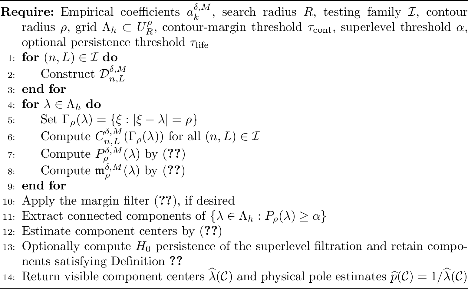
The parameters have separate roles. The contour radius \(\rho\) controls spatial resolution. Small \(\rho\) gives sharper but potentially fragmented responses, while large \(\rho\) smooths the field but may merge close poles. The threshold \(\alpha\) selects high-response visible clusters. The margin threshold \(\tau_{\rm cont}\) removes unstable contours. The persistence threshold \(\tau_{\rm life}\), when used, removes components that are short-lived across threshold levels.
Remark 5 (Scope and limitations). The method is a visible-cluster imaging and certification procedure. It does not guarantee recovery of every formal pole in the meromorphic model. The output is a set of fixed-threshold or persistent visible components in the reciprocal plane. A component may correspond to one pole, to several close poles that are not separated at the chosen radius, or to a feature that is visible only over a limited threshold range.
The main mechanisms that reduce visibility are small residues, large physical pole modulus, proximity to the boundary of \(U_R\), close reciprocal poles, holomorphic background terms comparable to the pole contribution, and noise that changes local winding counts. These are not limitations of the topological post-processing layer alone; they reflect the underlying stability balance between determinant perturbation and contour margin.
5 Numerical experiments↩︎
This section illustrates the contour-count indicator field and its use for visible-pole cluster extraction. The experiments are designed to test five questions: whether \(P_\rho\) behaves as an imaging functional, whether fixed thresholding can extract visible pole clusters, how the result depends on the contour radius and threshold, what persistent post-processing contributes, and how the method behaves in visibility-limited configurations.
Unless otherwise stated, the reciprocal search region is \[U_R=\{\lambda\in\mathbb{C}:1/R<|\lambda|<1\},\] and the indicator field is evaluated on a uniform Cartesian grid restricted to the shrunk annulus \(U_R^\rho\). The synthetic coefficient sequence has the form \[a_k = h_k+\sum_{j=1}^{N}c_j\lambda_j^k, \qquad k=0,1,\ldots ,\] with three reciprocal poles \[\lambda_1=0.8,\qquad \lambda_2=0.620998-0.299976\,\mathrm{i},\qquad \lambda_3=0.501485+0.307463\,\mathrm{i}.\] A holomorphic background and small complex coefficient noise are included. The testing family consists of several determinant orders and shifts, and \(P_\rho\) is computed from the fraction of local contours for which the argument-principle count equals one.
For localization accuracy, when the estimated and true numbers of visible clusters agree, we use the maximum matching error \[e_{\max} = \min_{\pi\in\mathfrak S_N} \max_{1\leq j\leq N} |\widehat\lambda_{\pi(j)}-\lambda_j|,\] where \(\mathfrak S_N\) denotes the set of permutations of \(\{1,\ldots,N\}\). When the numbers differ, we report the recovered components and interpret the result as a visibility-limited cluster count.
5.1 Indicator-field behavior↩︎
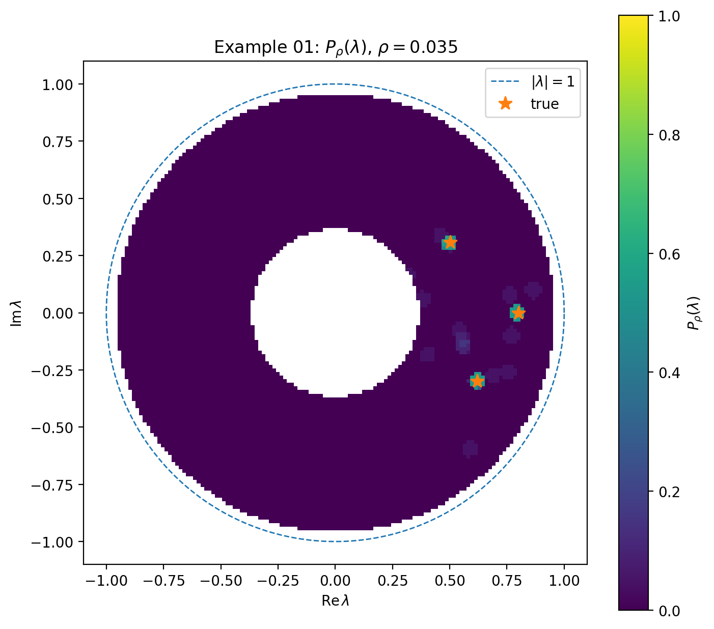
Figure 2 shows the contour-count indicator field \(P_\rho(\lambda)\) with \(\rho=0.035\). The field is concentrated near the three true reciprocal poles, while most of the search annulus has value close to zero. This confirms that the one-zero contour decisions, after averaging over determinant orders and shifts, produce a useful imaging functional on the reciprocal pole plane.
The high-response sets are not point masses. This is expected: a local circle centered at \(\lambda\) gives a one-zero response whenever the disk \(B(\lambda,\rho)\) contains one empirical determinant zero. Thus each pole generates a spatially extended response region whose width is controlled by \(\rho\) and by the spread of the empirical determinant zeros.
5.2 Fixed-threshold cluster extraction↩︎
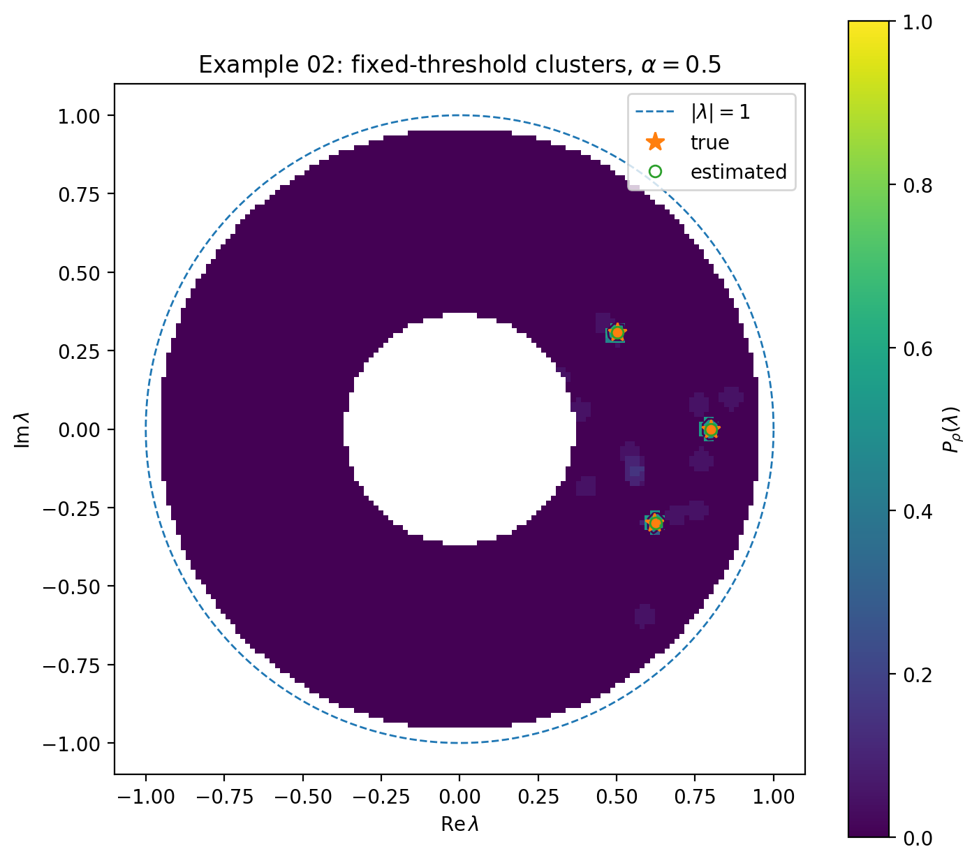
We next apply the fixed-threshold extraction rule \[\Omega_{\rho,\alpha} = \{\lambda\in U_R^\rho:P_\rho(\lambda)\geq\alpha\}.\] For \(\rho=0.035\) and \(\alpha=0.5\), the method extracts three connected components. Their weighted centers are listed in Table 1. The recovered centers are close to the three true reciprocal poles, with nearest-pole errors between \(5.08\times10^{-4}\) and \(4.20\times10^{-3}\).
| Rank | Size | Max \(P_\rho\) | Center \(\widehat\lambda\) | Median margin | Nearest error |
|---|---|---|---|---|---|
| 1 | 14 | 0.60 | \(0.501763+0.308801\,\ii\) | \(5.94\times10^{-9}\) | \(1.37\times10^{-3}\) |
| 2 | 15 | 0.55 | \(0.624934-0.298516\,\ii\) | \(4.49\times10^{-9}\) | \(4.20\times10^{-3}\) |
| 3 | 16 | 0.55 | \(0.799492-0.000000\,\ii\) | \(3.41\times10^{-9}\) | \(5.08\times10^{-4}\) |
Figure 3 displays the same indicator field together with the extracted component centers. The green circles overlap the true pole locations, showing that the fixed-threshold rule already gives reliable visible-pole localization in this example.
5.3 Dependence on the contour radius and threshold↩︎
The contour radius \(\rho\) controls the spatial scale of the indicator response. A small radius gives sharper responses but may fragment the field; a larger radius gives smoother responses but may merge nearby features. Figure 4 shows \(P_\rho\) for \[\rho=0.020,\;0.035,\;0.050,\;0.070 .\] The visible components remain centered near the true reciprocal poles over this range of radii, while the response regions broaden as \(\rho\) increases.
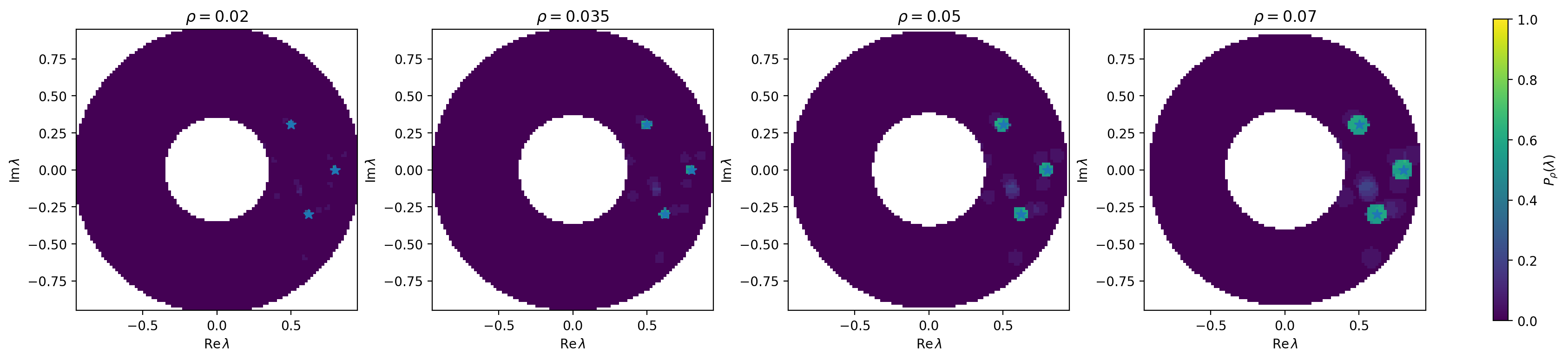
Table 2 reports the number of extracted components and the matching error for different combinations of \(\rho\) and threshold \(\alpha\). For \(\alpha=0.35\) and \(\alpha=0.50\), the method extracts the correct number of visible components for all tested radii. The matching error remains on the order of \(10^{-3}\). For \(\alpha=0.65\), no component is extracted because the threshold is above the observed peak level of the field in most cases. This illustrates why the threshold must be chosen relative to the attainable indicator height.
| \(\rho\) | \(\alpha\) | No. components | \(e_{\max}\) | Max \(P_\rho\) |
|---|---|---|---|---|
| 0.020 | 0.35 | 3 | \(2.976\times10^{-3}\) | 0.55 |
| 0.020 | 0.50 | 3 | \(2.976\times10^{-3}\) | 0.55 |
| 0.020 | 0.65 | 0 | – | 0.55 |
| 0.035 | 0.35 | 3 | \(3.100\times10^{-3}\) | 0.60 |
| 0.035 | 0.50 | 3 | \(4.745\times10^{-3}\) | 0.60 |
| 0.035 | 0.65 | 0 | – | 0.60 |
| 0.050 | 0.35 | 3 | \(5.174\times10^{-3}\) | 0.60 |
| 0.050 | 0.50 | 3 | \(5.174\times10^{-3}\) | 0.60 |
| 0.050 | 0.65 | 0 | – | 0.60 |
| 0.070 | 0.35 | 3 | \(4.075\times10^{-3}\) | 0.65 |
| 0.070 | 0.50 | 3 | \(4.302\times10^{-3}\) | 0.65 |
| 0.070 | 0.65 | 0 | – | 0.65 |
These results support the interpretation of \(P_\rho\) as a sampling-type indicator. The field gives stable visible-pole information over a moderate range of contour radii and thresholds, but an overly high threshold may remove all components.
5.4 Persistent post-processing↩︎
We then apply zero-dimensional persistence to the superlevel filtration of \(P_\rho\). This step is used as a post-processing tool, not as a replacement for fixed-threshold extraction. The corresponding persistence diagram is shown in Figure 5. The three dominant components have birth levels approximately \[0.60,\qquad 0.55,\qquad 0.55,\] and persist until the lowest background level in the discrete filtration. In contrast, many small components lie close to the diagonal or have short lifetimes, reflecting low-level spurious responses.
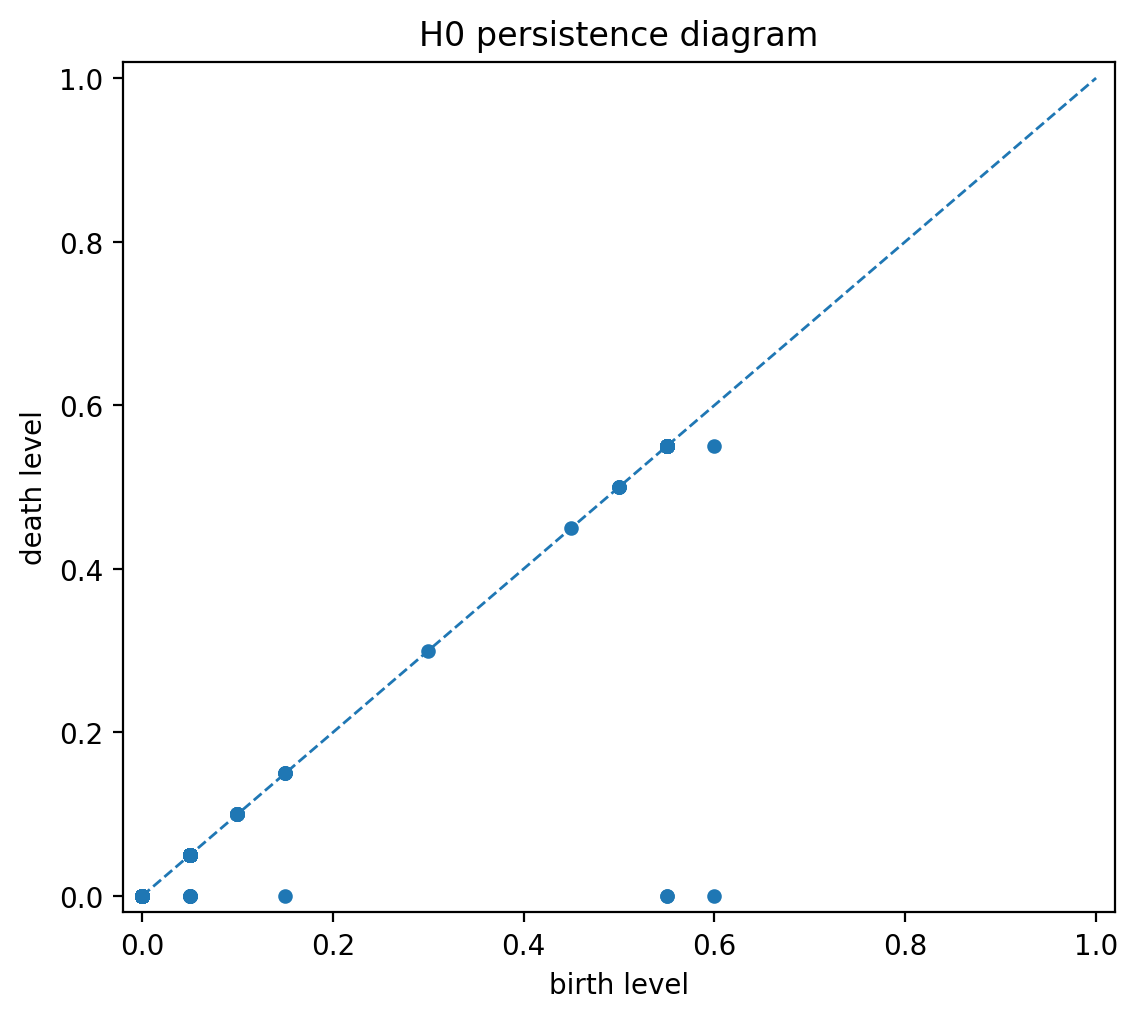
This experiment clarifies the role of persistent homology in the proposed framework. Fixed thresholding is sufficient when the high-response components are clearly separated from the background. Persistence becomes useful when one wants to reduce dependence on a particular value of \(\alpha\) and retain only components that survive over a range of thresholds.
5.5 Visibility limitations↩︎
Finally, we test three configurations where pole visibility is expected to degrade. The results are shown in Figure 6 and reported in Table 3.

| Case | No. components | Max \(P_\rho\) | Component centers |
|---|---|---|---|
| Small residue | 2 | 0.75 | \(0.798000+0.000934\,\ii;\;0.501238+0.305448\,\ii\) |
| Boundary-near pole | 2 | 0.65 | \(0.798178+0.000355\,\ii;\;0.623301-0.304841\,\ii\) |
| Close poles | 2 | 0.65 | \(0.722673-0.151664\,\ii;\;0.799462-0.000731\,\ii\) |
In the small-residue case, the weak pole does not produce a sufficiently strong high-response component at the chosen threshold. In the boundary-near case, the pole close to \(\partial U_R\) is difficult to certify because admissible contours are geometrically restricted and the determinant margin is reduced. In the close-pole case, two nearby reciprocal poles merge into a single visible component. These outcomes are consistent with the visible-cluster interpretation of the method: the algorithm reports stable clusters supported by the available contour-count evidence, rather than guaranteeing recovery of every formal pole.
Overall, the experiments support the proposed workflow. The contour-count indicator field localizes visible reciprocal poles, fixed-threshold superlevel components provide a direct extraction method, persistent homology serves as a threshold-robust post-processing tool, and the observed failures match the predicted visibility mechanisms.
6 Conclusions↩︎
We introduced a contour-count indicator field for visible pole clusters in outward meromorphic continuation. The field aggregates local argument-principle zero counts over determinant orders and shifts and can be interpreted as a sampling-type imaging functional in the reciprocal pole plane. Fixed superlevel sets provide direct visible-cluster extraction, while zero-dimensional persistent homology supplies an optional threshold-robust post-processing layer.
The analysis shows how pure-pole determinant factorization, one-zero contour geometry, Rouché stability, superlevel-set separation, and persistence-gap stability combine to explain the observed behavior of the indicator field. Strong isolated poles generate robust high-value components, while weak, close, boundary-near, or noise-dominated poles may produce low, short-lived, or merged responses.
Future work includes adaptive multiscale contour radii, sharper quantitative links between determinant margins and indicator-field contrast, and systematic comparisons with Hankel-pencil, Prony, Padé, AAA, and inverse-scattering-inspired sampling indicators.