The Benjamini–Hochberg Procedure Can Fail to Control the FDR for Correlated Two-Sided Gaussian Tests
July 13, 2026
Abstract
We show that the Benjamini–Hochberg procedure can fail to control the false discovery rate (FDR) at its nominal level for correlated two-sided Gaussian \(p\)-values. We construct a factor model for which, at level \(\alpha=0.01\), a rigorous interval-arithmetic certificate proves \(\operatorname{FDR}>0.0104\) for all sufficiently large numbers of hypotheses. This disproves a conjecture widely believed to be true for twenty years. Monte Carlo experiments are consistent with the theoretical result. The proof was obtained by GPT-5.6 Pro and carefully checked by the author.
1 The conjecture and the counterexample↩︎
Multiple hypothesis testing is a central topic in modern statistics, with applications in biology, genomics, astronomy, economics, finance, and many other fields. Over the last three decades, controlling the false discovery rate (FDR) [1] has become a standard target in applications involving many tests.
The Benjamini–Hochberg (BH) procedure is the standard method for FDR control. It controls the FDR when the \(p\)-values are independent [1], or when they satisfy the weaker positive regression dependence condition of [2]. See also [3]–[5] and the references below.
A crucial setting that had remained unresolved is that of correlated two-sided Gaussian tests. This setting matters because many data sets involve correlated tests; for example, neighboring genes or genetic variants can be correlated. Two-sided tests are also common because the direction of an effect is often unknown in advance, requiring simultaneous sensitivity to positive and negative effects.
In this paper we show, contrary to prior conjectures and supporting evidence [6], [7], that the Benjamini–Hochberg procedure need not control the FDR at its nominal level for correlated two-sided Gaussian tests.
More specifically, we consider the following setting. Let \(X\sim \mathcal{N}_m(\mu,\Sigma)\), where \(\Sigma\) is a correlation matrix. For \(1\le i\le m\), form the two-sided Gaussian \(p\)-value \(P_i=2\overline{\Phi}(|X_i|),\) where \(\Phi\) is the standard normal CDF and \(\overline{\Phi}=1-\Phi\). The Benjamini–Hochberg (BH) procedure [1] at level \(\alpha \in (0,1)\) uses critical values \(t_r=\alpha r/m\). Let \(R=\max\bigl\{r:\#\{i:P_i\le t_r\}\ge r\bigr\},\) with \(R=0\) if the set is empty. The BH procedure rejects those hypotheses \(H_i:\mu_i=0\) with \(P_i\le t_R\). If \(I_0=\{i:\mu_i=0\}\) denotes the true-null index set, define the number of false rejections by \(V=\#\{i\in I_0:P_i\le t_R\}.\) The false discovery proportion (FDP), the fraction of rejected hypotheses that are true nulls, is \(\operatorname{FDP}=V/\max(R,1)\), and the false discovery rate is its mean, \(\operatorname{FDR}=\mathbb{E}[\operatorname{FDP}]\).
A key question about the BH procedure is the following:
Does the Benjamini–Hochberg procedure control the false discovery rate at level \(\alpha\), i.e., do we have \(\operatorname{FDR}\le\alpha\), for every \(m\), every mean vector, every correlation matrix, and every \(\alpha\in(0,1)\)?
Before this work, a positive answer was widely believed. [6], [8] provided empirical and theoretical evidence in support of FDR control, and [9] provided additional evidence through extensive simulations. In an influential review, [7] wrote that “convincing simutheoretical evidence indicates that [FDR control] holds for two-sided z-tests with any correlation structure.” This motivates referring to the positive answer as a conjecture.
More recently, [10] wrote that “The answer to this question is generally believed to be yes, and is conjectured so in the literature since results of numerical studies investigating the question and reported in numerous papers strongly support it.” [10] continued that “proving this conjecture […] seems an urgent and important undertaking.” Similar statements were made by [11] and [12].
In this paper we show that the conjecture fails, by constructing the following Gaussian factor model. Let \(Z,\,(\varepsilon_i)_{i\ge1},\,(\eta_j)_{j\ge1},\,(\xi_k)_{k\ge1}\) be mutually independent standard normal random variables. For a fixed \(N\), define three coordinate blocks by \[\begin{align} X_i^{(0)} &=\frac{3}{10}Z+\frac{\sqrt{91}}{10}\varepsilon_i, &&1\le i\le96N,\tag{1}\\ X_j^{(1)} &=\frac{12}{5}-\frac{3}{10}Z+\frac{\sqrt{91}}{10}\eta_j, &&1\le j\le N,\tag{2}\\ X_k^{(2)} &=\frac{22}{5}-\frac{18}{25}Z+\frac{\sqrt{301}}{25}\xi_k, &&1\le k\le3N.\tag{3} \end{align}\] The block in 1 contains the \(96N\) true nulls. The other two blocks contain the \(4N\) nonnulls. The null block moves with \(Z\), whereas both signal blocks move against it, at two different strengths.
Theorem 1 (The Benjamini–Hochberg Procedure Can Fail to Control the FDR for Correlated Two-Sided Gaussian Tests). For each integer \(N\ge1\), let \(m_N=100N\), let the first \(96N\) hypotheses be true nulls, and let \(\operatorname{FDR}_N\) denote the FDR in the model above. Then the Benjamini–Hochberg procedure at level \(\alpha=0.01\) satisfies, for all sufficiently large \(N\), \[\operatorname{FDR}_N>0.0104>\alpha.\] Consequently, the conjecture is false.
Proof. The construction and all analytic details occupy the remainder of the paper. The final strict numerical inequality is established by the complete outward-rounded certificate in Appendix 10. ◻
1.0.0.1 AI usage.
The proof was obtained by GPT-5.6 Pro. The model was asked directly to prove or disprove the conjecture and was provided only with the mathematical definition of the Benjamini–Hochberg procedure. After about 90 minutes of reasoning, the model produced a proof, an example, and code for the numerical certificate, which form the basis of this paper.2 The author carefully checked the entire argument and the associated numerical certificate. Subsequently, the author asked the model to provide additional simulations, related work, and illustrations for a paper draft, and wrote the final version by editing the AI-generated draft.
Thus, this work falls into a line of work where AI models have helped professional mathematical scientists resolve open problems, see e.g., [13]–[23], etc.
2 Relation to existing FDR analysis↩︎
The conjecture lies between two classical regimes. Under mutual independence of the null \(p\)-values and independence from the nonnull \(p\)-values, ordinary BH satisfies the sharper bound \(\operatorname{FDR}\le\pi_0\alpha\), where \(\pi_0=|I_0|/m\) [1]. The same bound holds under positive regression dependence on the subset of true nulls (PRDS) [2]–[4].
By contrast, under completely arbitrary dependence the universal finite-sample guarantee for the unmodified linear step-up rule carries a harmonic inflation factor; replacing \(\alpha\) by \(\alpha/H_m\), where \(H_m=\sum_{r=1}^m r^{-1}\), restores level-\(\alpha\) control [2].
For one-sided Gaussian tests, nonnegative correlations provide an important PRDS setting [2], [3]. The two-sided transformation is qualitatively different: \(\{P_i\le t\}=\{X_i\ge c_t\}\cup\{X_i\le-c_t\}\) folds together two tails that induce opposite conditional shifts in correlated coordinates. Consequently, the usual monotone-regression and total-positivity arguments used for one-sided statistics do not automatically transfer to the folded Gaussian vector. This obstruction is discussed explicitly by [11] and [12].
Earlier work of [6] combined low-dimensional analysis, upper bounds, and simulation evidence, and [7] described the evidence for arbitrary-correlation control as “simutheoretical” while noting that a complete proof was unavailable. The later literature therefore developed dependence-adjusted or shifted alternatives with provable control rather than a proof for ordinary BH [10]–[12], [24].
Our argument uses a classical empirical CDF crossing representation of BH. In independent mixture models, and in several dependent asymptotic regimes, the random BH threshold is compared with the crossing of a limiting \(p\)-value CDF and the line \(t/\alpha\) [5], [25]–[27].
An innovation in our setting is the construction of a specific Gaussian factor model. Conditioning on a single latent factor produces three independent within-block empirical processes, but leaves a random limiting CDF \(G_Z\). The loadings and nonnull means are tuned so that, on a set of latent-factor values of positive Gaussian probability, the nonnull blocks enlarge the BH rejection count at precisely the same time that the conditional null distribution has heavier two-sided tails. This creates a self-consistent threshold with an FDP slightly above \(\alpha\).
A second innovation is that the argument avoids requiring a unique limiting crossing, differentiability at a crossing, or convergence of the BH threshold to an explicitly solved root. Two strict sign conditions merely bracket the threshold. Monotonicity of Gaussian tail probabilities then turns the continuum of \((z,c)\) values into finitely many rational rectangles, and outward-rounded ball arithmetic verifies the required signs. This combination of a one-sided threshold bracketing and a finite interval certificate is the distinctive mechanism of the proof.

3 Lemmas for the asymptotic BH threshold↩︎
In the remaining sections we present the argument of the proof. The proof is transparent in terms of empirical \(p\)-value distribution functions. Interpreting BH as the rightmost crossing of an empirical CDF and the line \(t/\alpha\) is standard in the asymptotic FDR literature [25]–[27]. The following lemma isolates the weaker one-sided bracketing fact that will be needed here.
For a sample of size \(M_N\), let \[\widehat G_N(t)=\frac{1}{M_N}\sum_{i=1}^{M_N}\mathbf{1}\{P_{i,N}\le t\}, \qquad 0\le t\le1.\] Let the BH grid be \(\mathcal{T}_N=\left\{\frac{\alpha r}{M_N}:1\le r\le M_N\right\},\) and define the BH \(p\)-value threshold \[\tau_N=\max\left( \left\{t\in\mathcal{T}_N:\widehat G_N(t)\ge\frac{t}{\alpha}\right\} \cup\{0\}\right).\] This is exactly \(\tau_N=\alpha R_N/M_N\): at the grid point \(t=\alpha r/M_N\), the inequality \(\widehat G_N(t)\ge t/\alpha\) is equivalent to having at least \(r\) \(p\)-values below the \(r\)th BH critical value. The argument will leverage the two lemmas below, whose proofs are presented in the appendix.
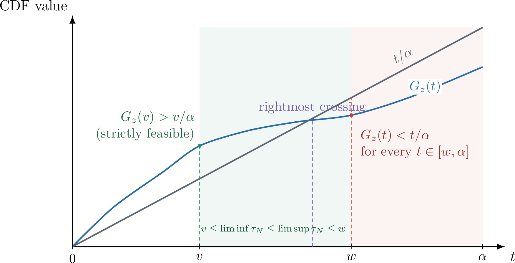
Lemma 1 (Two strict sign conditions bracket the BH threshold). Fix \(\alpha\in(0,1)\). Suppose \(M_N\to\infty\) and, for a continuous distribution function \(G\) on \([0,1]\), \(\|\widehat G_N-G\|_\infty\longrightarrow0.\) Let \(0<v\le w\le\alpha\). If \[G(t)<\frac{t}{\alpha} \quad\text{for every }t\in[w,\alpha], \label{eq:no-feasible}\tag{4}\] and \(G(v)>\frac{v}{\alpha}\), then \(\limsup_{N\to\infty}\tau_N\le w\) and \(\liminf_{N\to\infty}\tau_N\ge v\).
We also need the corresponding lower bound for the false discovery proportion. Suppose that \(|I_{0,N}|=\pi_0M_N\) for every \(N\), where \(\pi_0\in(0,1]\), and define the true-null empirical CDF \[\widehat F_{0,N}(t) =\frac{1}{\pi_0M_N}\sum_{i\in I_{0,N}}\mathbf{1}\{P_{i,N}\le t\}.\]
Lemma 2 (Threshold bracketing implies an FDP lower bound). In addition to the assumptions of Lemma 1, suppose \(\|\widehat F_{0,N}-F_0\|_\infty\longrightarrow0\) for a continuous CDF \(F_0\). Then \[\liminf_{N\to\infty}\operatorname{FDP}_N \ge \frac{\alpha\pi_0F_0(v)}{w}.\]
Figure 2 summarizes the geometry of Lemmas 1–2. Only a feasible point at \(v\) and a strictly infeasible terminal interval beginning at \(w\) are required.
4 Conditional limiting \(p\)-value distributions↩︎
We now recall the factor model introduced earlier. Let \(a_N\in\mathbb{R}^{100N}\) be the vector whose entries are \(3/10\) on the first block, \(-3/10\) on the second block, and \(-18/25\) on the third block. Let \(D_N\) be diagonal, with diagonal entries \(91/100\), \(91/100\), and \(301/625\) on the respective blocks. Then \(\Sigma_N=a_Na_N^{\mathsf T}+D_N.\) Since every diagonal entry of \(D_N\) is strictly positive, \(D_N\) and therefore \(\Sigma_N\) are positive definite. Moreover, \[\left(\frac{3}{10}\right)^2+\frac{91}{100}=1, \qquad \left(\frac{18}{25}\right)^2+\frac{301}{625}=1.\] Thus every diagonal entry of \(\Sigma_N\) is one, so \(\Sigma_N\) is a correlation matrix.
The mean vector is zero on the first block, \(12/5\) on the second block, and \(22/5\) on the third block. In particular, all nonnull means are positive. Every true-null coordinate is marginally \(\mathcal{N}(0,1)\), so its two-sided \(p\)-value is valid and uniform on \([0,1]\) marginally.
For \(c\ge0\), define \(u(c)=2\overline{\Phi}(c).\) Thus \(u\) is continuous and strictly decreasing from \(1\) to \(0\), and \(P_i\le u(c)\) exactly when \(|X_i|\ge c\). For \(a\ge0\) and \(s>0\), define \[Q(c;a,s) =\overline{\Phi}\left(\frac{c-a}{s}\right) +\overline{\Phi}\left(\frac{c+a}{s}\right). \label{eq:Q-def}\tag{5}\] If \(Y\sim \mathcal{N}(m,s^2)\), then \(\mathbb{P}(|Y|\ge c)=Q(c;|m|,s).\)
Conditional on \(Z=z\), the means and standard deviations in the three blocks are \[\begin{align} M_0(z)&=\frac{3z}{10}, &s_0&=\frac{\sqrt{91}}{10},\\ M_1(z)&=\frac{12}{5}-\frac{3z}{10}, &s_1&=\frac{\sqrt{91}}{10},\\ M_2(z)&=\frac{22}{5}-\frac{18z}{25}, &s_2&=\frac{\sqrt{301}}{25}. \end{align}\] Let \(F_{g,z}\) be the conditional \(p\)-value CDF in block \(g\). Equation 5 gives \[F_{g,z}(u(c))=Q(c;|M_g(z)|,s_g).\] Because the three block proportions are exactly \(0.96\), \(0.01\), and \(0.03\), the conditional limiting CDF of all \(p\)-values is \[G_z(u(c)) =0.96\cdot Q(c;|M_0(z)|,s_0) +0.01\cdot Q(c;|M_1(z)|,s_1) +0.03\cdot Q(c;|M_2(z)|,s_2). \label{eq:Gz}\tag{6}\] At \(\alpha=0.01\), define \[h_z(c)=G_z(u(c))-100u(c). \label{eq:hz}\tag{7}\] Thus \(h_z(c)\ge0\) is precisely the limiting BH feasibility condition at the \(p\)-value threshold \(u(c)\).
Conditional on \(Z=z\), the \(p\)-values are independent and identically distributed within each block. The Glivenko–Cantelli theorem [28] applied to each of the three blocks therefore gives \(\sup_{0\le t\le1}|\widehat G_N(t)-G_z(t)|\longrightarrow0\) almost surely under the conditional law given \(Z=z\). Applied to the null block, it also gives \[\sup_{0\le t\le1}|\widehat F_{0,N}(t)-F_{0,z}(t)|\longrightarrow0.\] By the existence of regular conditional laws and Fubini’s theorem, these two convergences hold jointly with unconditional probability one, with \(z\) replaced by the realized value \(Z\). All the limiting CDFs are continuous because the conditional Gaussian laws have strictly positive variances.
For later use, we record two monotonicity properties of \(Q\). For \(c,a\ge0\) and \(s>0\), \[\frac{\partial}{\partial c}Q(c;a,s) =-\frac{1}{s}\left\{ \phi\left(\frac{c-a}{s}\right) +\phi\left(\frac{c+a}{s}\right) \right\}<0,\] so \(Q\) is strictly decreasing in \(c\). Also, \[\frac{\partial}{\partial a}Q(c;a,s) =\frac{1}{s}\left\{ \phi\left(\frac{c-a}{s}\right) -\phi\left(\frac{c+a}{s}\right) \right\}\ge0.\] Indeed, \(|c-a|\le c+a\), and the standard normal density is decreasing as a function of the absolute value of its argument. Hence \(Q\) is nondecreasing in \(|m|\).
5 A finite collection of inequalities suffices↩︎
Let \(c_\alpha=\Phi^{-1}(1-\alpha/2).\) Since BH thresholds never exceed \(\alpha\), only \(c\ge c_\alpha\) is relevant. Partition \([-5,5]\) into the one thousand intervals \[B_k=\left[\frac{k}{100},\frac{k+1}{100}\right], \qquad -500\le k\le499.\] For \(g\in\{0,1,2\}\), define the exact extrema \[m_{g,k}^-=\min_{z\in B_k}|M_g(z)|, \qquad m_{g,k}^+=\max_{z\in B_k}|M_g(z)|.\] Because each \(M_g\) is affine, these extrema are obtained exactly from the two endpoints and, when the affine function changes sign on the interval, from the value zero.
Use the rational \(c\)-grid \(c_j=\frac{j}{1000}, \, 2575\le j\le10000.\) We provide below a numerical certificate that verifies \(u(c_{2575})>0.01\), equivalently \(c_{2575}<c_\alpha\), so this grid starts below the entire relevant \(c\)-domain.
For \(2575\le j<10000\), define \[\begin{align} U_{j,k} &=0.96\cdot Q(c_j;m_{0,k}^+,s_0) +0.01\cdot Q(c_j;m_{1,k}^+,s_1) +0.03\cdot Q(c_j;m_{2,k}^+,s_2) -100u(c_{j+1}). \label{eq:Ujk} \end{align}\tag{8}\] If \(z\in B_k\) and \(c\in[c_j,c_{j+1}]\), the monotonicities just proved imply \[Q(c;|M_g(z)|,s_g)\le Q(c_j;m_{g,k}^+,s_g),\] while the decrease of \(u\) gives \(-100u(c)\le-100u(c_{j+1})\). Therefore \[h_z(c)\le U_{j,k} \quad\text{on }B_k\times[c_j,c_{j+1}]. \label{eq:upper-rectangle}\tag{9}\]
Let \(j_k\) be the first grid index for which \(U_{j,k}\) is not certified to be strictly negative, and put \(a_k=c_{j_k}.\) Our numerical certificate verifies \(u(a_k)<\alpha\). In particular, \(j_k>2575\). Every preceding rectangle has \(U_{j,k}<0\), so \[h_z(c)<0 \quad\text{for every }z\in B_k \text{ and every }c\in[c_\alpha,a_k]. \label{eq:negative-prefix}\tag{10}\] The endpoint \(a_k\) is included because it is the right endpoint of the last strictly certified rectangle.
For \(j\ge j_k\), define the pointwise lower bound \[\begin{align} L_{j,k} &=0.96\cdot Q(c_j;m_{0,k}^-,s_0) +0.01\cdot Q(c_j;m_{1,k}^-,s_1) +0.03\cdot Q(c_j;m_{2,k}^-,s_2) -100u(c_j). \label{eq:Ljk} \end{align}\tag{11}\] Let \(\ell_k\ge j_k\) be the first index for which \(L_{\ell_k,k}\) is certified to be strictly positive, and put \(b_k=c_{\ell_k}.\) For every \(z\in B_k\), monotonicity in the absolute mean gives \[h_z(b_k)\ge L_{\ell_k,k}>0. \label{eq:positive-point}\tag{12}\] Because \(b_k\ge a_k\), one has \(u(b_k)\le u(a_k)<\alpha\).
Fix an outcome in the probability-one event on which both empirical-CDF convergences hold, and suppose that its realized factor value \(z=Z\) lies in \(B_k\). In Lemma 1, take \[v=u(b_k), \qquad w=u(a_k), \qquad G=G_z.\] As \(u\) is decreasing, condition 10 is exactly \(G_z(t)<100t=t/\alpha\) for every \(t\in[u(a_k),\alpha]\), and 12 is exactly \(G_z(u(b_k))>100u(b_k)\). Lemma 2, with \(\pi_0=0.96\), yields \[\liminf_{N\to\infty}\operatorname{FDP}_N \ge \frac{0.01\cdot0.96 \cdot F_{0,z}(u(b_k))}{u(a_k)}.\] Now \[F_{0,z}(u(b_k)) =Q(b_k;|M_0(z)|,s_0) \ge Q(b_k;m_{0,k}^-,s_0).\] Consequently, on this probability-one event, whenever \(Z\in B_k\), \[\liminf_{N\to\infty}\operatorname{FDP}_N\ge d_k, \qquad d_k=\frac{0.0096 Q(b_k;m_{0,k}^-,s_0)}{u(a_k)}. \label{eq:dk}\tag{13}\]
The finite reduction for one \(z\)-bin is shown in Figure 3. The upper bounds \(U_{j,k}\) certify a whole prefix of infeasible BH thresholds, whereas one lower bound \(L_{\ell_k,k}\) provides a feasible point farther out in the Gaussian-tail coordinate.
![Figure 3: One certified rectangle column B_k\times[c_\alpha,10].Monotonicity in c and in the absolute conditional means makes the displayedfinite sign checks valid uniformly over the entire bin.](/article/2607.12208/_pdflatex/fvhzmino.png "fig:")
6 The certified lower bound and completion of the proof↩︎
Every rational input to the certificate—the means, factor loadings, block weights, \(z\)-bin endpoints, and \(c\)-grid points—is specified using ratios of integers, without binary floating-point literals. The square roots defining the residual standard deviations and all Gaussian tails are evaluated as Arb balls. Arb performs outward-rounded midpoint-radius ball arithmetic [29]: every computed ball contains the exact real value. A strict comparison is accepted only when the entire resulting ball lies on the stated side of zero. Thus the tests \(U_{j,k}<0\), \(L_{j,k}>0\), \(u(c_{2575})>\alpha\), and \(u(a_k)<\alpha\) are rigorous interval statements, not floating-point heuristics.
The certificate computes the right side of \[\sum_{k=-500}^{499}d_k \left\{\Phi\left(\frac{k+1}{100}\right) -\Phi\left(\frac{k}{100}\right)\right\}. \label{eq:cert-sum}\tag{14}\] For readability, the one thousand terms are grouped into ten unit intervals. The following are certified strict lower bounds; every displayed decimal is rounded downward:
| Range of \(Z\) | Contribution to 14 |
|---|---|
| \([-5,-4]\) | \(0.000006254227057215695292015471184518827\) |
| \([-4,-3]\) | \(0.000116801968722543993192086605837856445\) |
| \([-3,-2]\) | \(0.000762743726482023098968624717496448543\) |
| \([-2,-1]\) | \(0.001839640615452850387738159572547846549\) |
| \([-1,0]\) | \(0.002006865275162943558353752660173437476\) |
| \([0,1]\) | \(0.001953237173075828884087571780890001262\) |
| \([1,2]\) | \(0.001827735787140664069157918588581283062\) |
| \([2,3]\) | \(0.001367544916156818165023914540138520994\) |
| \([3,4]\) | \(0.000508812722703075293268312075251660515\) |
| \([4,5]\) | \(0.000027192658519749972390210373148917831\) |
| Total on \([-5,5]\) | \(0.010416829070473713117472566385250491510\) |
Since \(0\le\operatorname{FDP}_N\le1\), Fatou’s lemma applies. The bins cover \([-5,5]\) up to endpoints of Gaussian probability zero. Equation 13 and the nonnegativity of the contribution from \(|Z|>5\) give \[\begin{align} \liminf_{N\to\infty}\operatorname{FDR}_N =\liminf_{N\to\infty}\mathbb{E}[\operatorname{FDP}_N] \ge\mathbb{E}\left[\liminf_{N\to\infty}\operatorname{FDP}_N\right] &\ge\sum_{k=-500}^{499}d_k\mathbb{P}(Z\in B_k) >0.0104. \end{align}\] This proves Theorem 1.
7 A Monte Carlo experiment↩︎
Here we provide a Monte Carlo experiment to support the theoretical analysis. However, a naive Monte Carlo experiment is inefficient: the conditional FDP is typically modest for central values of the common factor \(Z\), whereas uncommon factor values can produce much larger FDPs and make a nonnegligible contribution to the expectation. We therefore stratify on \(Z\) while simulating every residual coordinate and recomputing the BH rule without approximation.
Let \(K=1000\) and define the equiprobable standard-normal strata \[I_k=\left(\Phi^{-1}\left(\frac{k-1}{K}\right), \Phi^{-1}\left(\frac{k}{K}\right)\right], \qquad 1\le k\le K,\] with the usual interpretations at probabilities zero and one. In macro-replication \(b\), draw independently \[U_{b,k}\sim\operatorname{Unif}\left(\frac{k-1}{K},\frac{k}{K}\right), \qquad Z_{b,k}=\Phi^{-1}(U_{b,k}),\] one draw from each stratum. Conditional on each \(Z_{b,k}\), generate all \(100N\) Gaussian coordinates from 1 –3 , form the two-sided \(p\)-values, sort them, apply ordinary BH at \(\alpha=0.01\) exactly, and record the resulting \(D_{b,k,N}=\operatorname{FDP}_{b,k,N}\). The macro-replication estimate is \(Y_{b,N}=\frac{1}{K}\sum_{k=1}^K D_{b,k,N}.\) Because every stratum has probability \(1/K\) and \(Z_{b,k}\) has the conditional law of \(Z\) given \(Z\in I_k\), \[\mathbb{E}[Y_{b,N}] =\frac{1}{K}\sum_{k=1}^K\mathbb{E}[\operatorname{FDP}_N\mid Z\in I_k] =\mathbb{E}[\operatorname{FDP}_N] =\operatorname{FDR}_N.\] Thus stratification changes the Monte Carlo variance but not the estimand. We used \(B=100\) independent macro-replications and reported \(\widehat{\operatorname{FDR}}_N=\frac{1}{B}\sum_{b=1}^B Y_{b,N}\), \(\widehat{\operatorname{MCSE}} =\frac{s_Y}{\sqrt B},\) where \(s_Y\) is the sample standard deviation of the \(Y_{b,N}\). The intervals below are conventional Student-\(t\) Monte Carlo intervals with \(B-1=99\) degrees of freedom.
The experiment used \(100{,}000\) complete Gaussian data sets at each dimension. The retained reproducibility bundle uses Python 3.12.3, NumPy 1.26.4, SciPy 1.14.1, and python-flint 0.8.0. The complete executable and the macro-replication outputs are available in the GitHub repository at https://github.com/dobriban/BH.
| \(N\) | \(m\) | \(\widehat{\operatorname{FDR}}_N\) | MCSE | \(95\%\) MC interval | \(p_+\) |
|---|---|---|---|---|---|
| \(50\) | \(5{,}000\) | \(0.009936\) | \(0.000113\) | \([0.009711,\,0.010161]\) | \(0.713\) |
| \(100\) | \(10{,}000\) | \(0.010129\) | \(0.000096\) | \([0.009939,\,0.010320]\) | \(0.0905\) |
| \(200\) | \(20{,}000\) | \(0.010359\) | \(0.000103\) | \([0.010155,\,0.010563]\) | \(3.56\times10^{-4}\) |
Here \(p_+\) denotes the one-sided Student-\(t\) Monte Carlo \(p\)-value for the null inequality \(\operatorname{FDR}_N\le0.01\).
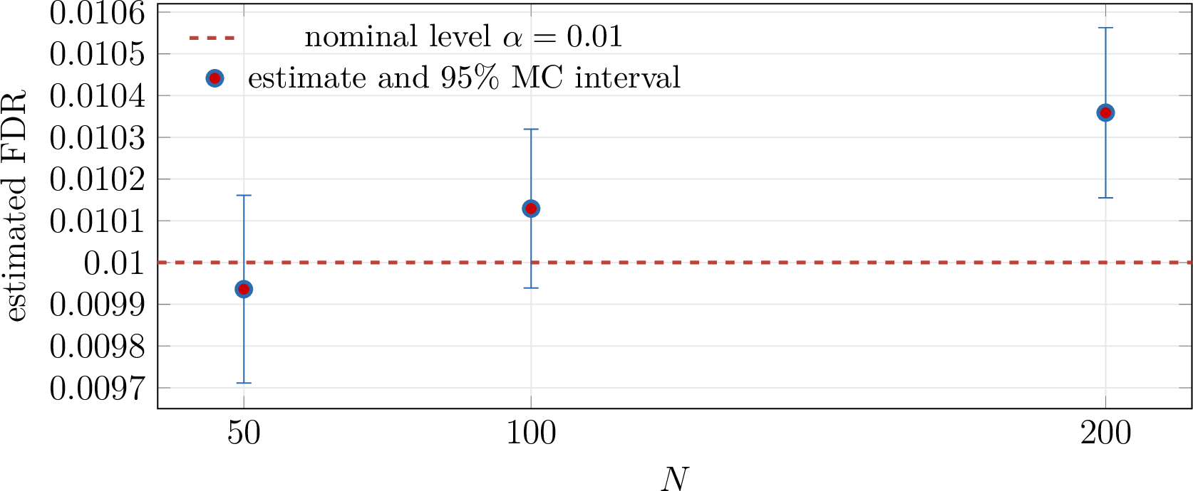
At \(N=200\), the excess is \(\widehat{\operatorname{FDR}}_{200}-\alpha=0.0003589\), or about \(3.59\%\) of the nominal level. The corresponding statistic is \(3.495\) Monte Carlo standard errors above \(\alpha\), giving the one-sided \(p\)-value in the table. Thus the direct finite-dimensional experiment provides evidence of the same failure of control established asymptotically. At \(N=50\) and \(N=100\), the intervals still overlap the nominal level. This may be because more Monte Carlo replications are needed, or because the true finite-sample FDR does not exceed the nominal level at those dimensions.
8 Discussion↩︎
Several points merit further study. The example above violates the nominal level only slightly, and additional numerical searches over related models have found similarly small violations. This raises the question of whether a universal bound exists on the possible inflation of the FDR above its nominal level.
Moreover, the example uses a large number of tests. It is therefore important to determine whether the BH procedure is guaranteed to control the FDR for smaller numbers of tests and, if not, to obtain bounds that depend explicitly on the number of tests. Both questions are directions for future research.
9 Proofs↩︎
9.1 Proof of Lemma 1↩︎
Proof. Set \(H(t)=G(t)-t/\alpha\). By continuity and the strict inequality 4 , the maximum of \(H\) on the compact interval \([w,\alpha]\) is a strictly negative number. Hence there is an \(\varepsilon>0\) such that \(H(t)\le-2\varepsilon \quad\text{for all }t\in[w,\alpha].\) For all sufficiently large \(N\), uniform convergence gives \(\|\widehat G_N-G\|_\infty<\varepsilon\). Therefore \[\widehat G_N(t)-\frac{t}{\alpha} \le H(t)+\varepsilon \le-\varepsilon<0\] for every \(t\in[w,\alpha]\). No BH grid point in that interval is feasible, which proves \(\limsup_N\tau_N\le w\).
For the lower bound, \(G(v)>\frac{v}{\alpha}\) and continuity give a \(\delta>0\) and an open interval \(J\) containing \(v\) such that \(H(t)\ge2\delta\) for all \(t\in J\). The mesh of \(\mathcal{T}_N\) is \(\alpha/M_N\to0\), so one can choose \(s_N\in\mathcal{T}_N\cap J\) with \(s_N\to v\). For all sufficiently large \(N\), uniform convergence gives \[\widehat G_N(s_N)-\frac{s_N}{\alpha} \ge H(s_N)-\delta \ge\delta>0.\] Thus \(s_N\) is feasible, and the maximal feasible grid point obeys \(\tau_N\ge s_N\). Taking lower limits proves \(\liminf_N\tau_N\ge v\). ◻
9.2 Proof of Lemma 2↩︎
Proof. Lemma 1 gives \(\liminf_N\tau_N\ge v>0\), so eventually \(\tau_N>0\). By the definition of the BH threshold, \(R_N=\frac{M_N\tau_N}{\alpha}.\) The number of false rejections is \(V_N=\pi_0M_N\widehat F_{0,N}(\tau_N).\) Consequently, \[\operatorname{FDP}_N =\frac{V_N}{R_N} =\frac{\alpha\pi_0\widehat F_{0,N}(\tau_N)}{\tau_N}. \label{eq:fdp-threshold-identity}\tag{15}\] For every \(\varepsilon\in(0,v)\), the inequality \(\tau_N\ge v-\varepsilon\) holds eventually. Monotonicity of empirical CDFs and uniform convergence then give \(\liminf_{N\to\infty}\widehat F_{0,N}(\tau_N) \ge F_0(v-\varepsilon).\) Letting \(\varepsilon\downarrow0\) and using continuity of \(F_0\) yields \(\liminf_{N\to\infty}\widehat F_{0,N}(\tau_N)\ge F_0(v).\) For any \(\varepsilon>0\), these two bounds imply, eventually, \(\widehat F_{0,N}(\tau_N)\ge F_0(v)-\varepsilon\) and \(\tau_N\le w+\varepsilon\). Substitution in 15 gives \[\operatorname{FDP}_N\ge \frac{\alpha\pi_0\{F_0(v)-\varepsilon\}}{w+\varepsilon}.\] Letting \(\varepsilon\downarrow0\) proves the result. ◻
10 Complete outward-rounded certificate↩︎
The following Python program is the complete numerical certificate used above. It requires python-flint 0.8.0. The specialization to the exact grids used in the proof deliberately avoids floating-point conversion in all mathematical inputs
and all grid-index calculations.
#!/usr/bin/env python3
"""Outward-rounded certificate for the two-sided Gaussian BH counterexample.

Dependency: python-flint

All model parameters and all subdivision endpoints are exact rationals.
Every transcendental evaluation is an Arb ball with outward rounding.
"""

from flint import arb, ctx

ctx.dps = 40

ALPHA = arb(1) / 100
PI0 = arb(24) / 25
W1 = arb(1) / 100
W2 = arb(3) / 100
R0 = arb(3) / 10
R1 = -arb(3) / 10
R2 = -arb(18) / 25
MU1 = arb(12) / 5
MU2 = arb(22) / 5
S0 = (1 - R0 * R0).sqrt()
S1 = (1 - R1 * R1).sqrt()
S2 = (1 - R2 * R2).sqrt()
SQRT2 = arb(2).sqrt()

Z_DEN = 100
C_DEN = 1000
K_MIN = -500
K_MAX = 500
J_START = 2575
J_STOP = 10000


def normal_upper_tail(x: arb) -> arb:
    return (x / SQRT2).erfc() / 2


def normal_cdf(x: arb) -> arb:
    return 1 - normal_upper_tail(x)


def two_sided_tail(c: arb, abs_mean: arb, sd: arb) -> arb:
    return (
        normal_upper_tail((c - abs_mean) / sd)
        + normal_upper_tail((c + abs_mean) / sd)
    )


def p_threshold(c: arb) -> arb:
    return 2 * normal_upper_tail(c)


def abs_range_of_affine(
    mu: arb, loading: arb, lo: arb, hi: arb
) -> tuple[arb, arb]:
    left = mu + loading * lo
    right = mu + loading * hi
    abs_left = abs(left)
    abs_right = abs(right)
    if (left <= 0 and right >= 0) or (right <= 0 and left >= 0):
        minimum = arb(0)
    else:
        minimum = abs_left if abs_left < abs_right else abs_right
    maximum = abs_left if abs_left > abs_right else abs_right
    return minimum, maximum


def certify_bin(k: int) -> arb:
    z_lo = arb(k) / Z_DEN
    z_hi = arb(k + 1) / Z_DEN

    m0_lo, m0_hi = abs_range_of_affine(arb(0), R0, z_lo, z_hi)
    m1_lo, m1_hi = abs_range_of_affine(MU1, R1, z_lo, z_hi)
    m2_lo, m2_hi = abs_range_of_affine(MU2, R2, z_lo, z_hi)

    c_start = arb(J_START) / C_DEN
    assert p_threshold(c_start) > ALPHA

    j_lower = None
    for j in range(J_START, J_STOP):
        c_j = arb(j) / C_DEN
        c_next = arb(j + 1) / C_DEN
        h_upper = (
            PI0 * two_sided_tail(c_j, m0_hi, S0)
            + W1 * two_sided_tail(c_j, m1_hi, S1)
            + W2 * two_sided_tail(c_j, m2_hi, S2)
            - 100 * p_threshold(c_next)
        )
        if not (h_upper < 0):
            j_lower = j
            break
    if j_lower is None:
        raise RuntimeError(f"No lower bracket in z-bin {k}")

    c_lower = arb(j_lower) / C_DEN
    # This is equivalent to c_lower > c_alpha and ensures that at least
    # one preceding cell was rigorously certified negative.
    assert p_threshold(c_lower) < ALPHA

    j_upper = None
    for j in range(j_lower, J_STOP + 1):
        c_j = arb(j) / C_DEN
        h_lower = (
            PI0 * two_sided_tail(c_j, m0_lo, S0)
            + W1 * two_sided_tail(c_j, m1_lo, S1)
            + W2 * two_sided_tail(c_j, m2_lo, S2)
            - 100 * p_threshold(c_j)
        )
        if h_lower > 0:
            j_upper = j
            break
    if j_upper is None:
        raise RuntimeError(f"No feasible point in z-bin {k}")

    c_upper = arb(j_upper) / C_DEN
    fdp_lower = (
        (PI0 / 100)
        * two_sided_tail(c_upper, m0_lo, S0)
        / p_threshold(c_lower)
    )
    gaussian_mass = normal_cdf(z_hi) - normal_cdf(z_lo)
    return fdp_lower * gaussian_mass


def main() -> None:
    total = arb(0)
    unit_totals: dict[int, arb] = {}

    for k in range(K_MIN, K_MAX):
        contribution = certify_bin(k)
        total += contribution
        unit = k // Z_DEN
        unit_totals[unit] = unit_totals.get(unit, arb(0)) + contribution

    for unit in sorted(unit_totals):
        print(f"z in [{unit},{unit + 1}]: {unit_totals[unit]}")
    print(f"certified total over [-5,5]: {total}")

    assert total > arb("0.0104168290704737131174725663852504915")
    assert total > ALPHA
    print(
        "CERTIFIED: liminf FDR > "
        "0.0104168290704737131174725663852504915 > alpha = 0.01"
    )


if __name__ == "__main__":
main()References↩︎
Department of Statistics and Data Science, University of Pennsylvania. E-mail address:
dobriban@wharton.upenn.edu.↩︎The conversation is available as a shared ChatGPT conversation.↩︎