Rzk: a Proof Assistant for Synthetic \(\infty\)-Categories
July 13, 2026
Abstract
Homotopy type theory (HoTT) is a type theory that allows for synthetic reasoning about \(\infty\)-groupoids. Several proof assistants (such as Rocq and Agda) implement variants of HoTT.
Directed type theory is a type theory for synthetic reasoning about \(\infty\)-categories, where morphisms (or paths) of dimension 1 are not necessarily invertible. Among the proposals for directed type theory, the most developed is Riehl and Shulman’s simplicial type theory (RSTT), based on simplicial shapes such as directed intervals and triangles.
We present Rzk, a proof assistant implementing (a refinement of) RSTT for synthetic reasoning about \(\infty\)-categories. Specifically, the type theory implemented by Rzk is a computational variant of RSTT adjusted to make type checking practical.
We define a translation from RSTT to Rzk and prove that it is sensible: every RSTT proof translates to an Rzk proof (faithfulness), and Rzk proves nothing new about RSTT types (conservativity). We also give a tutorial introduction to proving in Rzk, and describe its implementation, including the type-checking algorithm and the automated prover for the logic of shapes.
<ccs2012> <concept> <concept_id>10003752.10003790.10003794</concept_id> <concept_desc>Theory of computation Automated reasoning</concept_desc> <concept_significance>500</concept_significance> </concept> <concept> <concept_id>10003752.10003790.10011740</concept_id> <concept_desc>Theory of computation Type theory</concept_desc> <concept_significance>500</concept_significance> </concept> </ccs2012>
1 Introduction↩︎
In this paper, we describe the proof assistant Rzk1. Rzk implements a simplicial type theory similar to the one developed by [1] (RSTT). That type theory supports synthetic reasoning about \((\infty,1)\)-categories, much as homotopy type theory (HoTT) supports synthetic reasoning about \((\infty,0)\)-categories. We give a precise account of the type theory that Rzk implements, and relate it to RSTT via a translation that we prove faithful and, on a natural fragment of derivations, conservative. At its core, Rzk is roughly RSTT extended by a few declarative refinements, together with the algorithmisation that makes type checking effective: \[\begin{array}{@{}r@{\;\;}l@{\qquad}l@{\;\;}l@{\;}l@{\;\;}l@{\;}l@{}} & \text{\textsf{RSTT}{}} & & \rdelim\}{3}{2pt} & \multirow{3}{*}{~Declarative \textsf{Rzk}{}} & \rdelim\}{6}{2pt} & \multirow{6}{*}{~Algorithmic \textsf{Rzk}{}}\\[2pt] + & \text{split extension types} & \text{(\ref{sec:sec:split-ext})}\\ + & \text{coercion-free subtyping} & \text{(\ref{sec:subtyping} \ref{sec:checking-subtyping})}\\[4pt] + & \text{first-class parameters} & \text{(\ref{sec:sec:tope-params})}\\ + & \text{bidirectional typing} & \text{(\ref{sec:bidirectional} \ref{sec:def-eq-topes})}\\ + & \text{an automated tope solver} & \text{(\ref{sec:sec:automated-tope-logic})} \end{array}\] The first two refinements are declarative and are the subject of 4; the last three concern the implementation, described in 6. We also give a tutorial on proving in Rzk, in 2.
1.1 Background on Type Theories and Their Interpretations↩︎
In this section, we put simplicial type theory in the context of HoTT, to motivate both the type theory itself and a proof assistant for it.
Dependent type theory (or “type theory” for short), developed by [2] and [3], provides the logical basis for many proof assistants. A special feature of type theory is the inductively specified identity type proposed by Martin-Löf as a suitable notion of equality: given \(a, a' : A\), the type \(a =_{A}a'\) collects witnesses of “sameness” of \(a\) and \(a'\), and, being itself a type, it can be iterated. [4] interpret types as groupoids and thereby show that the principle of “Uniqueness of Identity Proofs” is not provable: two “parallel” identities \(p, q : a =_{A}a'\) need not be identical. HoTT takes this insight further, interpreting types as \(\infty\)-groupoids: objects, invertible morphisms, morphisms between morphisms, and so on in every dimension. Voevodsky’s univalence axiom completes this interpretation: with it, type theory has types of every homotopy level [5], and proof assistants can reason synthetically about “spaces”, that is, \(\infty\)-groupoids. Cubical type theories [6]–[8] regain the canonicity property lost by adding univalence as an axiom.
An \(\infty\)-category has morphisms of every dimension, of which the morphisms of dimension 1 need not be invertible, while the “higher” morphisms, such as morphisms between morphisms, are. Explicitly, \(\infty\)-categories are also called \((\infty,1)\)-categories, and \(\infty\)-groupoids are the \((\infty,0)\)-categories. Such \(\infty\)-categories arise in the study of homotopy theory, but also in the syntax of type theory: a syntactic universe should carry the structure of an \(\infty\)-category whose objects are types, whose 1-morphisms are functions, and whose higher morphisms are terms of identity type. For these reasons, soon after the development of HoTT, a quest began to reason synthetically not just about \(\infty\)-groupoids, but also about \(\infty\)-categories. In such a type theory, a type \(A\) representing an \(\infty\)-category comes, in particular, with a type \(\hom_A(x,y)\) of morphisms from \(x\) to \(y\) for any \(x,y:A\).
[1] develop such a type theory: a type theory with shapes whose special case, simplicial type theory (RSTT), supports synthetic reasoning about \((\infty,1)\)-categories. In RSTT, the types that can be interpreted as \((\infty,1)\)-categories are the Rezk types: types whose morphisms compose (Segal types) and whose isomorphisms coincide with identities. A distinguishing feature of RSTT is the extension type, a type of functions that behave in a specified way on part of the domain, up to definitional equality. In particular, extension types provide the hom-types: in RSTT, \(\hom_A(x,y)\) is the type of functions from the directed interval \(\mathbb{2}\) that return \(x\) at \(0\) and \(y\) at \(1\), definitionally. Because such boundary conditions hold definitionally, they carry no propositional bookkeeping in proofs. We review RSTT in 3.1, and the tutorial of 2 builds towards Rezk types.
1.2 This Paper: Theory and Practice of Rzk↩︎
In this paper, we present a proof assistant called Rzk, which implements a variant of RSTT.
Rzk has seen real use. Its “standard library”, sHoTT [9] (7.1), comprises over 25 000 lines and nearly 1 500 top-level declarations of synthetic \((\infty,1)\)-category theory, developing Segal and Rezk types, covariant families, adjunctions, cocartesian fibrations, and (co)limits. Rzk enabled the first formalisation of the \(\infty\)-categorical Yoneda lemma, by Kudasov, Riehl, and Weinberger [10]. The master’s thesis of Lossin [11] develops cocartesian fibrations in synthetic \((\infty,1)\)-category theory, formalising its results in Rzk and contributing parts of them to sHoTT. Rzk and sHoTT were taught at a summer school in Regensburg in 2023,2 and the upcoming ICERM workshop “Teaching Higher Category Theory with Computers” (August 2026)3 builds its practical sessions on Rzk. Two ongoing developments build on Rzk: a proof-game engine in the style of the Lean 4 games [12], whose first game is the work-in-progress Yoneda game,4 and modal extensions of Rzk towards directed univalence [13].
We present Rzk from two perspectives. From the practical perspective, we give a short tutorial on using Rzk in 2, and report on larger-scale type-checking performance of Rzk in 7. From the theoretical perspective, we present declarative Rzk (dRzk for short) in 4, and compare it to RSTT in 5 by defining a translation from RSTT to dRzk and proving it faithful and, on a natural fragment of derivations, conservative. In 6 we present algorithmic Rzk (aRzk for short), the “computational” variant of dRzk, featuring a bidirectional type-checking algorithm and an automated tope solver. It is the basis of the implementation of Rzk.
One technical obstacle to a precise comparison is that Riehl and Shulman state their theorems schematically, over an abstract context of cubes, topes, and tope inclusions. Rzk internalises these data as first-class parameters of a definition (6.2). We therefore make the meta-level assumptions formal as a meta-theoretic parameter layer (MPL) surrounding RSTT (3.2). Statements of dRzk are schematic over the same layer, and our translation keeps it in place.
Stating the algorithm precisely paid off in practice. Auditing the implementation against the rules of 18 uncovered two soundness bugs in released versions of Rzk, through v0.7.7: the checker equated identity types without comparing their underlying types, and the asymmetric subtype checks ran in a fixed direction, hence backwards in negative positions, such as the domain of a \(\Pi\)-type. Both bugs are fixed in v0.7.8, the version reported in this paper; see 5 for details, including the migration the first fix required in the sHoTT library.5
2 Proving in Rzk↩︎
In this section, we walk through a sequence of Rzk definitions6, building up to a Rezk type, the synthetic \((\infty,1)\)-category (2.5). The full code of every example is in the ancillary files accompanying this paper. Most examples have counterparts in sHoTT [9] (a community library of synthetic \((\infty,1)\)-category theory written in Rzk, evaluated in 7.1), which we point to as we go. After each example, we note which of Rzk’s simplicial features (if any) are invoked behind the scenes. Further examples are collected in 11.
2.1 The Martin-Löf Fragment↩︎
One layer of Rzk is Martin-Löf type theory, in standard notation: is the type of dependent functions from to , with for the non-dependent case and for the universe7; is the type of dependent pairs ; and is the identity type, inhabited by whenever the two sides are definitionally equal, and eliminated by path induction (). Warm-up examples in this fragment are collected in 11: the polymorphic and functions, the projections out of a \(\Sigma\)-type, and a proof by that is its own inverse, which typechecks because Rzk \(\eta\)-expands on demand (6.3). None of these examples involves a simplicial feature of Rzk.
2.2 Cubes, Topes, and Extension Types↩︎
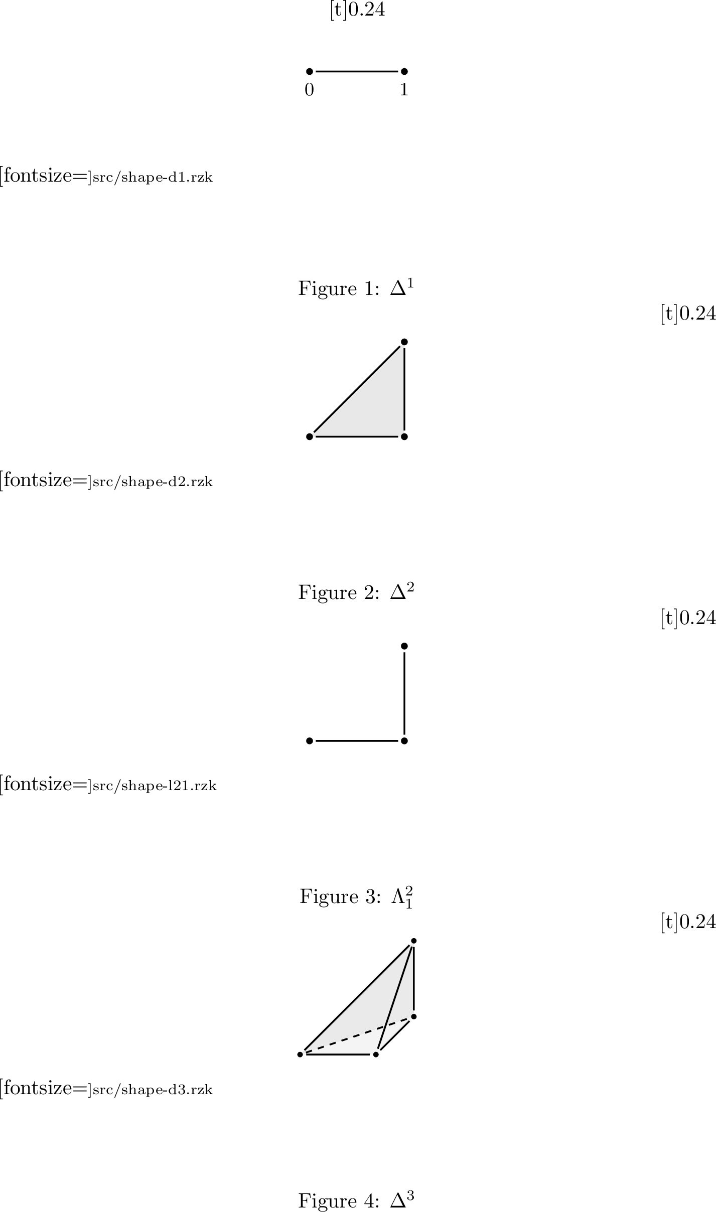
The simplicial layer of Rzk adds two ingredients below the types (3.1). A cube is an abstract space of points. The basic cube is the directed interval, carrying a total order with distinct least and greatest points and . Cubes can be multiplied: is the cube of pairs of points, so is the directed square. A tope is a logical formula constraining the points of a cube, built from equations , inequalities , the connectives and , and the constants (true) and (false). A cube together with a tope carves out a shape. 1 shows the four shapes that recur throughout the paper and their Rzk definitions: the 1-simplex is the whole interval (the always-true tope ); the 2-simplex is the triangle cut out of the square by ; the inner horn keeps only the two edges of meeting at vertex \(1\); and the 3-simplex is the tetrahedron cut out of the 3-cube by .
Functions may take a shape as their domain, and the extension type prescribes such a function on part of its domain. Given a shape , a subshape (a tope entailing ), and a section defined over , the extension type, written in Rzk, is the type of functions from to that agree with on definitionally: computes to whenever holds, with no proof obligation and no explicit coercion. The rest of this section shows extension types at work.
2.3 Hom-Types and Directed Paths↩︎
Mapping shapes into a type lets us view some types as synthetic \((\infty,1)\)-categories. A -type is the type of morphisms between two elements and of a type : a mapping from the 1-simplex to with definitionally fixed endpoints ( maps to , maps to ). The same pattern, one dimension up, gives a -type: a mapping from the 2-simplex to whose three boundary edges are pinned to three given s , , . An inhabitant is thus a filled triangle witnessing that the composite of and agrees with . 2 shows both, together with their Rzk definitions.
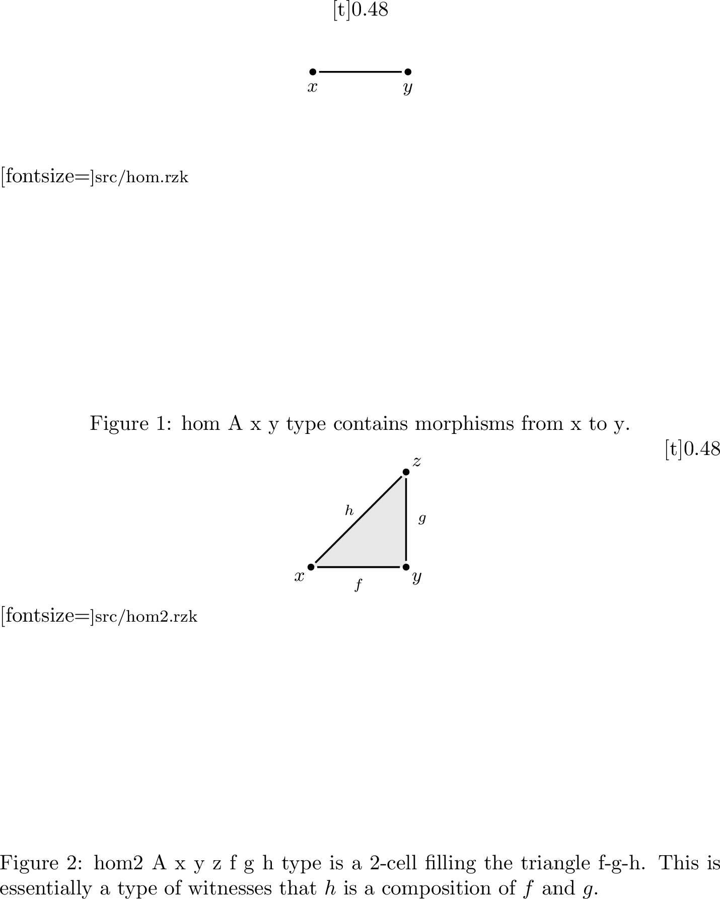
Here the simplicial layer of Rzk is used for the first time. The bracketed restriction on is the type restriction of 4.2. When a term of type is applied at the endpoint , Rzk rewrites the application to , and at to (6.3). The implied tope side conditions (e.g.that the boundary is included in the shape ) are checked automatically by the tope solver of 6.5. The same two mechanisms make the three boundaries of compute: applying a 2-cell on the edge yields , on the edge yields , and on the diagonal yields . Where two edges meet, the branches must agree; e.g., at the corner both and compute to .
2.4 Cofibration Composition↩︎
None
Figure 3: Cofibration composition in Rzk..
The examples so far used shapes to carve simplicial structure out of a type . Rzk can also prove theorems about the shape machinery itself, schematic in a cube, topes over it, and a type family, with no simplicial reading attached. For example, a theorem of [1], the composition law for cofibrations, states that an extension type from a tope to a larger factors through any intermediate with \(\phi \vdash \psi \vdash \chi\)8: extending from to is equivalent to extending from to and then from to . The Rzk statement and proof are in 3. Both maps re-package the same underlying section, and both round-trips are witnessed by .
The forward map sends a section to the pair : the same , used once as an extension over the smaller shape and once as a further extension from to . The witnesses are written \(\eta\)-expanded, as Riehl and Shulman write them in their proof: the second component uses at a type whose boundary pins the values of itself, and this use is correct for but not for an arbitrary section of its type, so no subtyping between the two types can allow it (4).
The inverse map is the plain projection . Here Rzk’s coercion-free subtyping (4.3) accepts , a section with boundary , where one with boundary is expected, with no coercion inserted. Unlike in the forward direction, this passage is correct for every section of ’s type: the expected boundary sits on the smaller tope ( entails ), and wherever holds the two boundaries agree definitionally, since there computes to and to .
Here, the round-trip witnesses typecheck because each composite reduces to the identity: applying a section pinned on a tope at a point where that tope holds computes to the pin (the restriction computation of 6.3), and the tope solver proves the entailments \(\phi(t) \vdash \psi(t)\) and \(\psi(t) \vdash \chi(t)\) from the parameter structure (6.5). Neither the subtyping step nor these computations appear in the proof term.
2.5 \(\infty\)-Categories↩︎
A Segal type is a synthetic pre-\(\infty\)-category: every composable pair of its morphisms has a unique composite. Promoting it to a synthetic \((\infty,1)\)-category, that is,
a Rezk type, requires the additional completeness condition: every type-theoretic identity arises from a unique isomorphism in the Segal structure on . Segal-ness matters here, since only it makes composition, and hence invertibility of a
morphism, well-defined. In sHoTT, module simplicial-hott/10-rezk-types, the definition reads:
#lang rzk-1

#def is-rezk (A : U) : U
  := Σ ( is-segal-A : is-segal A)
     , ( x : A) → (y : A)
     → is-equiv (x = y) (Iso A is-segal-A x y) (iso-eq A is-segal-A x y)
The \(\Sigma\) unpacks as follows: is Segal, and for every pair \((x, y)\) of points the canonical map from to (which sends to the identity isomorphism by path induction) is an equivalence. Up to equivalence, identities in are exactly the isomorphisms.
Both Segal-ness and Rezk-ness lift along the function-type formers [1]; the corresponding sHoTT closure lemmas are shown in 11.5.
Here, the entire Rezk predicate is built from extension types and \(\Sigma\) over the type and tope layers. The type-directed restriction computation of 6.3 applies whenever an -witness is unpacked at an endpoint or used to interpret an isomorphism, and the tope solver checks the simplex- and horn-inclusion side conditions arising in the underlying Segal component (6.5). Thus, Rzk can express, and mechanically check, the synthetic \((\infty,1)\)-categorical condition itself. The sHoTT library [9] contains a growing body of synthetic \(\infty\)-category theory built on this foundation, including the first formalisation of the \(\infty\)-categorical Yoneda lemma [10].
3 RSTT Review and the Meta-Theoretic Parameter Layer↩︎
In this section, we review RSTT(3.1) and then formalise, as a meta-theoretic parameter layer (MPL, 3.2), the meta-level assumptions under which theorems are stated by [1]. We denote by MPL+ RSTT the formal system consisting of MPL and RSTT. In contrast to the literal Rzk code of 2, use math-mode notation, with the cube, tope, and type layers distinguished by colour.
3.1 Review of RSTT↩︎
RSTT [1] is a three-layered type theory: the first two layers are a coherent logic of cubes and topes (formulas built from atoms by \({\color{RoyalBlue}\wedge}\), \({\color{RoyalBlue}\vee}\), \({\color{RoyalBlue}\top}\), and \({\color{RoyalBlue}\bot}\), with no implication or negation), and the third layer is Martin-Löf type theory over the first two [1]. Accordingly a judgement carries up to three telescopic contexts, \[\Xi \mid \Phi \mid \Gamma \vdash J,\] a cube context \(\Xi\), a tope context \(\Phi\), and an ordinary type context \(\Gamma\). For example, the judgement \[{\color{BurntOrange}t} : {\color{Brown}\mathbb{2}} \;\mid\; {\color{BurntOrange}t} {\color{RoyalBlue}\equiv} {\color{BurntOrange}0} \;\mid\; x : {\color{OliveGreen}A},\;y : {\color{OliveGreen}A},\;f : \hom_{{\color{OliveGreen}A}}(x, y) \;\vdash\; f({\color{BurntOrange}t}) \equiv x : {\color{OliveGreen}A}\] binds a point of the directed interval in the cube context, assumes the tope \({\color{BurntOrange}t} {\color{RoyalBlue}\equiv} {\color{BurntOrange}0}\) in the tope context, and binds three typed variables in the type context; its conclusion is the definitional equality that 2.3 computed at an endpoint, with the hom-type defined in 1 below. Judgements of the lower layers use a prefix of the three contexts: a tope entailment, for instance, has the form \({\color{Brown}\Xi} \mid {\color{RoyalBlue}\Phi} \vdash {\color{RoyalBlue}\psi}\). We recall the layers and their judgement forms; for the inference rules we refer to the original paper [1].
3.1.0.1 Cubes.
The cube layer is a simply-typed theory whose types, the cubes, comprise a terminal cube \({\color{Brown}\mathbb{1}}\) (with unique point \({\color{BurntOrange}\star}\)), the directed interval \({\color{Brown}\mathbb{2}}\) (with two distinguished points \({\color{BurntOrange}0}, {\color{BurntOrange}1} : {\color{Brown}\mathbb{2}}\)), and binary products \({\color{Brown}I \times J}\). A cube context \({\color{Brown}\Xi}\) binds points \({\color{BurntOrange}t} : {\color{Brown}I}\), and the judgement \({\color{Brown}\Xi} \vdash {\color{BurntOrange}t} : {\color{Brown}I}\) asserts that \({\color{BurntOrange}t}\) is a point of the cube \({\color{Brown}I}\) in context \({\color{Brown}\Xi}\). Note that in RSTT a context cannot posit an abstract cube: abstraction over cubes (and over topes) happens only at the meta level.
3.1.0.2 Topes.
Over the cube layer sits an intuitionistic propositional logic of topes. A tope is a formula built from \({\color{RoyalBlue}\top}\), \({\color{RoyalBlue}\bot}\), conjunction \({\color{RoyalBlue}\wedge}\), and disjunction \({\color{RoyalBlue}\vee}\), together with two kinds of atomic formulas: equalities \({\color{BurntOrange}s} {\color{RoyalBlue}\equiv} {\color{BurntOrange}t}\) of points \({\color{BurntOrange}s}, {\color{BurntOrange}t} : {\color{Brown}I}\) of a cube, and inequalities \({\color{BurntOrange}s} {\color{RoyalBlue}\leq} {\color{BurntOrange}t}\) of points \({\color{BurntOrange}s}, {\color{BurntOrange}t} : {\color{Brown}\mathbb{2}}\). A tope context \({\color{RoyalBlue}\Phi}\) in cube context \({\color{Brown}\Xi}\) is a finite list of topes built from the points bound in \({\color{Brown}\Xi}\). The layer has two judgement forms: \({\color{Brown}\Xi} \vdash {\color{RoyalBlue}\phi} \;{\color{RoyalBlue}\mathsf{tope}}\) asserts that \({\color{RoyalBlue}\phi}\) is a well-formed tope over \({\color{Brown}\Xi}\), and the entailment \({\color{Brown}\Xi} \mid {\color{RoyalBlue}\Phi} \vdash {\color{RoyalBlue}\psi}\) asserts that \({\color{RoyalBlue}\psi}\) is entailed by \({\color{RoyalBlue}\Phi}\). The interval \({\color{Brown}\mathbb{2}}\) is totally ordered: any two points are comparable (\(\vdash {\color{BurntOrange}s} {\color{RoyalBlue}\leq} {\color{BurntOrange}t} {\color{RoyalBlue}\vee} {\color{BurntOrange}t} {\color{RoyalBlue}\leq} {\color{BurntOrange}s}\)), \({\color{BurntOrange}0}\) is least and \({\color{BurntOrange}1}\) greatest (\({\color{BurntOrange}0} {\color{RoyalBlue}\leq} {\color{BurntOrange}t}\) and \({\color{BurntOrange}t} {\color{RoyalBlue}\leq} {\color{BurntOrange}1}\) for every \({\color{BurntOrange}t} : {\color{Brown}\mathbb{2}}\)), and the endpoints are distinct (\({\color{BurntOrange}0} {\color{RoyalBlue}\equiv} {\color{BurntOrange}1} \vdash {\color{RoyalBlue}\bot}\)) [1]. Tope entailments are treated as side conditions whose derivations are left implicit.
3.1.0.3 Shapes and types.
A shape is a pair \(\{{\color{BurntOrange}t} : {\color{Brown}I} \mid {\color{RoyalBlue}\phi}\}\) of a cube \({\color{Brown}I}\) and a tope \({\color{RoyalBlue}\phi}\) in context \({\color{BurntOrange}t} : {\color{Brown}I}\), denoting the points of \({\color{Brown}I}\) satisfying \({\color{RoyalBlue}\phi}\). The type layer is Martin-Löf type theory (\({\color{OliveGreen}\Pi}\) over types, \({\color{OliveGreen}\Sigma}\), identity types, the unit type, \(\ldots\)) over \({\color{Brown}\Xi} \mid {\color{RoyalBlue}\Phi}\), with the usual judgements \({\color{Brown}\Xi} \mid {\color{RoyalBlue}\Phi} \mid {\color{OliveGreen}\Gamma} \vdash {\color{OliveGreen}A} \;{\color{OliveGreen}\mathsf{type}}\), \({\color{Brown}\Xi} \mid {\color{RoyalBlue}\Phi} \mid {\color{OliveGreen}\Gamma} \vdash a : {\color{OliveGreen}A}\), and definitional equality \({\color{Brown}\Xi} \mid {\color{RoyalBlue}\Phi} \mid {\color{OliveGreen}\Gamma} \vdash a \equiv b : {\color{OliveGreen}A}\). Note that a shape is not itself a type of this layer: functions out of a shape are provided by the extension types below, and there is no type of shapes.
3.1.0.4 Extension types.
Functions whose domain is a shape are provided by the extension type, the distinguishing feature of RSTT. Suppose we are given a shape \(\{{\color{BurntOrange}t} : {\color{Brown}I} \mid {\color{RoyalBlue}\psi}\}\), a subshape \(\{{\color{BurntOrange}t} : {\color{Brown}I} \mid {\color{RoyalBlue}\phi}\}\) (so that \({\color{BurntOrange}t} : {\color{Brown}I} \mid {\color{RoyalBlue}\phi} \vdash {\color{RoyalBlue}\psi}\)), a family \({\color{OliveGreen}A}\) over \(\{{\color{BurntOrange}t} : {\color{Brown}I} \mid {\color{RoyalBlue}\psi}\}\), and a term \(a : {\color{OliveGreen}A}\) defined over the subshape, that is, \({\color{BurntOrange}t} : {\color{Brown}I} \mid {\color{RoyalBlue}\phi} \mid {\color{OliveGreen}\Gamma} \vdash a : {\color{OliveGreen}A}\). The extension type \[\left\langle \prod\nolimits_{{\color{BurntOrange}t} : {\color{Brown}I} \mid {\color{RoyalBlue}\psi}} {\color{OliveGreen}A} \middle\vert \phantom{}^{{\color{RoyalBlue}\phi}}_{a} \right\rangle\] is the type of functions \(f\) defined over the whole shape that agree with \(a\) on the subshape definitionally: \(f({\color{BurntOrange}t}) \equiv a({\color{BurntOrange}t})\) whenever \({\color{RoyalBlue}\phi}({\color{BurntOrange}t})\) holds9. Imposing boundaries by definitional equality in this way greatly reduces bookkeeping in proofs. 9 (12) collects the typing rules for extension types (formation, introduction, application, \(\beta\), boundary computation, and \(\eta\)).
Example 1 (Hom-types). The prototypical extension type is the type of morphisms of \({\color{OliveGreen}A}\) from \(x\) to \(y\) (cf.the Rzk definition of in 2.3), \[\hom_{{\color{OliveGreen}A}}(x, y) \;:=\; \left\langle \prod\nolimits_{{\color{BurntOrange}t} : {\color{Brown}\mathbb{2}}} {\color{OliveGreen}A} \middle\vert \phantom{}^{{\color{BurntOrange}t} {\color{RoyalBlue}\equiv} {\color{BurntOrange}0} {\color{RoyalBlue}\vee} {\color{BurntOrange}t} {\color{RoyalBlue}\equiv} {\color{BurntOrange}1}}_{\mathsf{rec}_{{\color{RoyalBlue}\vee}}({\color{BurntOrange}t} {\color{RoyalBlue}\equiv} {\color{BurntOrange}0} \mapsto x, {\color{BurntOrange}t} {\color{RoyalBlue}\equiv} {\color{BurntOrange}1} \mapsto y)} \right\rangle,\] where the boundary section, assembled by tope disjunction elimination \(\mathsf{rec}_{{\color{RoyalBlue}\vee}}\), takes the value \(x\) at \({\color{BurntOrange}t} {\color{RoyalBlue}\equiv} {\color{BurntOrange}0}\) and \(y\) at \({\color{BurntOrange}t} {\color{RoyalBlue}\equiv} {\color{BurntOrange}1}\).
Hom-types are the main ingredient in the definition of Rezk types, the types that represent synthetic \((\infty,1)\)-categories: one reasons about a type \({\color{OliveGreen}A}\) through its hom-types, whose terms are the morphisms between its elements. [1] isolate the Rezk types in two stages: the Segal types, in which composable morphisms have unique composites, and the Rezk types themselves, Segal types whose isomorphisms moreover coincide with their identities [14]. The tutorial defines them in 2.5.
Remark 1 (Notational conventions for extension types). Riehl and Shulman state two notational conventions for extension types [1]. First, an extension type whose boundary tope is \({\color{RoyalBlue}\bot}\) “behaves just like an ordinary (possibly dependent) function type”, so the angle brackets are omitted: one writes \({\color{OliveGreen}\prod}_{{\color{BurntOrange}t} : {\color{Brown}I} \mid {\color{RoyalBlue}\psi}} {\color{OliveGreen}A}\) for \(\left\langle \prod\nolimits_{{\color{BurntOrange}t} : {\color{Brown}I} \mid {\color{RoyalBlue}\psi}} {\color{OliveGreen}A} \middle\vert \phantom{}^{{\color{RoyalBlue}\bot}}_{\mathsf{rec}_{{\color{RoyalBlue}\bot}}} \right\rangle\). Second, officially the codomain \({\color{OliveGreen}A}\) and the boundary \(a\) are a type and a term in the extended context \({\color{BurntOrange}t} : {\color{Brown}I} \mid {\color{RoyalBlue}\psi} \mid {\color{OliveGreen}\Gamma}\); the convention writes them as if they were functions applied to the shape variable, \({\color{OliveGreen}A}({\color{BurntOrange}t})\) and \(a({\color{BurntOrange}t})\), as in \(\left\langle \prod\nolimits_{{\color{BurntOrange}t} : {\color{Brown}I} \mid {\color{RoyalBlue}\psi}} {\color{OliveGreen}A}({\color{BurntOrange}t}) \middle\vert \phantom{}^{{\color{RoyalBlue}\phi}}_{a({\color{BurntOrange}t})} \right\rangle\). Both conventions return in 4: the first becomes literal in the split extension types of 4.2, and the second in the tope families and first-class parameters of 6.2, which turn the informal application notation into actual functions.
3.2 Meta-Theoretic Parameter Layer for RSTT↩︎
Statements in RSTT may rest on assumptions that live in the meta-theory rather than inside RSTT. This concerns not just assumptions such as “let \({\color{OliveGreen}A}\) be a type”, but also entailments between topes, such as a shape inclusion \({\color{BurntOrange}t} : {\color{Brown}I} \mid {\color{RoyalBlue}\phi} \vdash {\color{RoyalBlue}\psi}\) attached to a theorem as a side condition. As a concrete example, the composition law for cofibrations [1] opens with “suppose \({\color{BurntOrange}t} : {\color{Brown}I} \mid {\color{RoyalBlue}\phi} \vdash {\color{RoyalBlue}\psi}\) and \({\color{BurntOrange}t} : {\color{Brown}I} \mid {\color{RoyalBlue}\psi} \vdash {\color{RoyalBlue}\chi}\), and that \({\color{OliveGreen}X} : \{{\color{BurntOrange}t} : {\color{Brown}I} \mid {\color{RoyalBlue}\chi}\} \to {\color{OliveGreen}\mathcal{U}}\)”, and then asserts, for any \(a : {\color{OliveGreen}\prod}_{{\color{BurntOrange}t} : {\color{Brown}I} \mid {\color{RoyalBlue}\phi}} {\color{OliveGreen}X}({\color{BurntOrange}t})\), an equivalence \[\left\langle \prod\nolimits_{{\color{BurntOrange}t} : {\color{Brown}I} \mid {\color{RoyalBlue}\chi}} {\color{OliveGreen}X}({\color{BurntOrange}t}) \middle\vert \phantom{}^{{\color{RoyalBlue}\phi}}_{a} \right\rangle \;\simeq\; {\color{OliveGreen}\sum}_{f : \left\langle \prod\nolimits_{{\color{BurntOrange}t} : {\color{Brown}I} \mid {\color{RoyalBlue}\psi}} {\color{OliveGreen}X}({\color{BurntOrange}t}) \middle\vert \phantom{}^{{\color{RoyalBlue}\phi}}_{a} \right\rangle} \left\langle \prod\nolimits_{{\color{BurntOrange}t} : {\color{Brown}I} \mid {\color{RoyalBlue}\chi}} {\color{OliveGreen}X}({\color{BurntOrange}t}) \middle\vert \phantom{}^{{\color{RoyalBlue}\psi}}_{f} \right\rangle.\] The section \(a\) and the equivalence are an ordinary RSTT hypothesis and conclusion, respectively, but the cube \({\color{Brown}I}\), the three topes, their two entailments, and the family \({\color{OliveGreen}X}\) do not live in an RSTT context.
To define a formal translation from RSTT to dRzk, we need to formalise these meta-theoretic assumptions. We do this by defining the meta-theoretic parameter layer (MPL). An element of MPL is a meta-theoretic parameter context: it collects the schematic parameters and the side conditions that a statement is abstracted over.
Specifically, a meta-theoretic parameter context has five kinds of entries:
Definition 1 (Meta-theoretic parameter context). A meta-theoretic parameter context* is a dependent list of entries of the following kinds, each well-formed relative to the entries before it; an entry may depend on any earlier one, regardless of kind, so the kinds need not be grouped.*
**Cube parameters* \({\color{Brown}I_1}, \ldots, {\color{Brown}I_m}\), each positing an abstract cube (“let \({\color{Brown}I}\) be a cube”). From these one forms cube contexts \({\color{Brown}\Xi}\), the finite lists of points of the declared cubes.*
**Tope parameters \({\color{RoyalBlue}\phi_1}, \ldots, {\color{RoyalBlue}\phi_n}\), each positing an abstract tope over such a cube context, \({\color{Brown}\Xi} \vdash {\color{RoyalBlue}\phi_j} \;{\color{RoyalBlue}\mathsf{tope}}\).
**Tope inclusion assumptions, a finite list of entailments \({\color{Brown}\Xi} \mid {\color{RoyalBlue}\phi} \vdash {\color{RoyalBlue}\psi}\) between declared topes sharing a cube context \({\color{Brown}\Xi}\).
**Term parameters \(v_1 : {\color{OliveGreen}T_1}, \ldots, v_k : {\color{OliveGreen}T_k}\), each positing a variable of a previously formed type, \({\color{Brown}\Xi} \mid {\color{RoyalBlue}\Phi} \mid {\color{OliveGreen}\Gamma} \vdash {\color{OliveGreen}T} \;{\color{OliveGreen}\mathsf{type}}\) (“let \(a : {\color{OliveGreen}A}\)”). A type-family parameter cannot live in an RSTT context, and neither can the terms mentioned in its type. Term parameters lift such terms to the meta level, so that a later type-family parameter may depend on them.
**Type-family parameters* \(B_1, \ldots, B_l\), each positing a type over a cube context, \({\color{Brown}\Xi} \mid {\color{RoyalBlue}\Phi} \mid {\color{OliveGreen}\Gamma} \vdash B \;{\color{OliveGreen}\mathsf{type}}\), for some tope context \({\color{RoyalBlue}\Phi}\) over \({\color{Brown}\Xi}\) and some type context \({\color{OliveGreen}\Gamma}\) well-formed under \({\color{Brown}\Xi} \mid {\color{RoyalBlue}\Phi}\) and the earlier entries.*
An RSTT statement is schematic over* a meta-theoretic parameter context when it is an RSTT judgement in which the declared cubes, topes, and type families may occur, under the inclusion assumptions. An instance replaces each parameter by concrete RSTT data: a cube for each cube parameter, a tope for each tope parameter, a term for each term parameter, and a type family for each type-family parameter. To be an instance, the data must make every inclusion assumption a derivable RSTT entailment.*
Note that a type-family parameter is, by the convention above, usually written as a function into the universe, with the cube context packed into a single shape over the product cube as the domain: \(B : \{({\color{BurntOrange}t}, {\color{BurntOrange}s}) : {\color{Brown}I \times J} \mid {\color{BurntOrange}t} {\color{RoyalBlue}\leq} {\color{BurntOrange}s}\} \to ({\color{OliveGreen}x} : {\color{OliveGreen}A}) \to {\color{OliveGreen}\mathcal{U}}\) stands for the meta-judgement \({\color{BurntOrange}t} : {\color{Brown}I}, {\color{BurntOrange}s} : {\color{Brown}J} \mid {\color{BurntOrange}t} {\color{RoyalBlue}\leq} {\color{BurntOrange}s} \mid {\color{OliveGreen}x} : {\color{OliveGreen}A} \vdash B \;{\color{OliveGreen}\mathsf{type}}\). This is a notational convenience, not an RSTT function type.
Example 2 (The composition law for cofibrations). Consider again the composition law for cofibrations, proved in Rzk in 2.4. Its hypotheses form a meta-theoretic parameter context: one cube \({\color{Brown}I}\); three topes \({\color{RoyalBlue}\chi}, {\color{RoyalBlue}\psi}, {\color{RoyalBlue}\phi}\) over \({\color{Brown}I}\) with the inclusion assumptions \({\color{BurntOrange}t} : {\color{Brown}I} \mid {\color{RoyalBlue}\phi} \vdash {\color{RoyalBlue}\psi}\) and \({\color{BurntOrange}t} : {\color{Brown}I} \mid {\color{RoyalBlue}\psi} \vdash {\color{RoyalBlue}\chi}\); and one type-family parameter \({\color{OliveGreen}X} : \{{\color{BurntOrange}t} : {\color{Brown}I} \mid {\color{RoyalBlue}\chi}\} \to {\color{OliveGreen}\mathcal{U}}\). The remaining hypothesis and the conclusion are then ordinary RSTT judgements schematic over this context. An instance is a concrete cube with concrete topes that satisfy the two inclusions, recovering one instance of the Riehl–Shulman statement.
Example 3 (Dependent Yoneda). The dependent Yoneda lemma [1] is a directed analogue of path induction: for a Segal type \({\color{OliveGreen}A}\), an element \(a : {\color{OliveGreen}A}\), and a covariant family \({\color{OliveGreen}C} : (x : {\color{OliveGreen}A}) \to \hom_{{\color{OliveGreen}A}}(a, x) \to {\color{OliveGreen}\mathcal{U}}\), a dependent function in \({\color{OliveGreen}\prod}_{x : {\color{OliveGreen}A}} {\color{OliveGreen}\prod}_{f : \hom_{{\color{OliveGreen}A}}(a, x)} {\color{OliveGreen}C}(x, f)\) is determined, up to equivalence, by its value at the identity morphism of \(a\). For our purposes, the lemma illustrates a term parameter and a type family depending on it: its parameter context consists of a type-family parameter \({\color{OliveGreen}A} : {\color{OliveGreen}\mathcal{U}}\), term parameters \(\sigma : \mathsf{isSegal}({\color{OliveGreen}A})\) and \(a : {\color{OliveGreen}A}\), and the type-family parameter \({\color{OliveGreen}C}\) (whose covariance is a further term parameter). Because \({\color{OliveGreen}C}\) is a meta-theoretic parameter, it cannot mention a variable bound in an RSTT judgement. Thus \(a\) must itself be a term parameter declared before \({\color{OliveGreen}C}\), rather than a hypothesis of the RSTT statement.
4 Declarative Rzk↩︎
This section describes declarative Rzk (dRzk): RSTT extended by two refinements, as shown in the display of 1. First, dRzk splits the extension type of RSTT into two independent constructs whose combination recovers it: split extension types (4.2). This makes the first notational convention of 1 literal. Second, paper proofs in RSTT silently identify terms of different types, for instance reading an extension type as the plain function over its shape by forgetting its boundary. dRzk formalises these passages by an explicit coercion-free subtyping relation (4.3).10 dRzk shares its judgement forms and contexts with RSTT, so a dRzk statement can be schematic over a meta-theoretic parameter context (1) in exactly the same sense as an RSTT one. The implementation additionally internalises that layer, binding cubes, tope families, and type families as first-class parameters of a definition (6.2). 2 (10) summarises the correspondence, pairing each informal practice of RSTT with the Rzk device that formalises it.
4.1 Judgements and Contexts in Rzk↩︎
Before turning to Rzk’s refinements, we fix the judgement forms. Declarative Rzk keeps RSTT’s three context layers. A judgement has the form \({\color{Brown}\Xi} \mid {\color{RoyalBlue}\Phi} \mid {\color{OliveGreen}\Gamma} \vdash \mathcal{C}\), with a cube context \({\color{Brown}\Xi}\), a tope context \({\color{RoyalBlue}\Phi}\) of assumed topes, and a type context \({\color{OliveGreen}\Gamma}\); the conclusion \(\mathcal{C}\) can be
a type formation,
a typing \(M : {\color{OliveGreen}T}\),
a definitional equality \(t_1 \equiv t_2\), or
a subtyping \({\color{OliveGreen}A} \mathrel{<:}{\color{OliveGreen}B}\),
where the first three are like in RSTT(3.1).
4.2 Adding Split Extension Types↩︎
In place of RSTT’s extension-type former, which fuses the function type with its boundary, Rzk provides two independent constructs whose combination recovers extension types.
The first is the shape-indexed function type \({\color{OliveGreen}\prod}_{{\color{BurntOrange}t} : \{{\color{Brown}I} \mid {\color{RoyalBlue}\psi}\}} {\color{OliveGreen}B}\), the type of dependent functions over a shape \(\{{\color{Brown}I} \mid {\color{RoyalBlue}\psi}\}\), which recovers RSTT’s empty-boundary extension type (rule \(\Pi\)-form-shape in 4).
The second is a type restriction \({\color{OliveGreen}B}\,[\, {\color{RoyalBlue}\phi} \mapsto a \,]\), which attaches a definitional boundary to an arbitrary type \({\color{OliveGreen}B}\). It is well-formed when the boundary section \(a\) is well-typed under \({\color{RoyalBlue}\phi}\) (rule Restr-form in 4).
An element of this restriction is an element \(x : {\color{OliveGreen}B}\) that equals \(a\) wherever \({\color{RoyalBlue}\phi}\) holds (rule Restr-intro in 4). Whenever the tope context \({\color{RoyalBlue}\Phi}\) entails \({\color{RoyalBlue}\phi}\), such an \(x\) computes to \(a\) (rule Restr-comp in 4); this type-directed computation makes boundaries definitional.
The reason to split the extension-type former is that type checking produces intermediate types that have one construct without the other. Applying a section of an extension type at a point consumes the function part of the type, but must not forget its boundary: the natural type of the result is the codomain with a restriction on it, a type that RSTT cannot express and dRzk can. 4 shows such an intermediate type arising from the hom-type.
Example 4 (The hom-type, split). The hom-type of 1 reads in dRzk as a shape-\({\color{OliveGreen}\Pi}\) with a restricted codomain (the translation of 5.1 makes this reading official), \[\hom_{{\color{OliveGreen}A}}(x, y) \;=\; {\color{OliveGreen}\prod}_{{\color{BurntOrange}t} : \{{\color{Brown}\mathbb{2}} \mid {\color{RoyalBlue}\top}\}} \big( {\color{OliveGreen}A}\,[\, {\color{BurntOrange}t} {\color{RoyalBlue}\equiv} {\color{BurntOrange}0} {\color{RoyalBlue}\vee} {\color{BurntOrange}t} {\color{RoyalBlue}\equiv} {\color{BurntOrange}1} \mapsto \mathsf{rec}_{{\color{RoyalBlue}\vee}}({\color{BurntOrange}t} {\color{RoyalBlue}\equiv} {\color{BurntOrange}0} \mapsto x, {\color{BurntOrange}t} {\color{RoyalBlue}\equiv} {\color{BurntOrange}1} \mapsto y) \,]\big).\] Applying a morphism \(f\) at a point \({\color{BurntOrange}s}\) then yields the restricted* type \({\color{OliveGreen}A}\,[\, {\color{BurntOrange}s} {\color{RoyalBlue}\equiv} {\color{BurntOrange}0} {\color{RoyalBlue}\vee} {\color{BurntOrange}s} {\color{RoyalBlue}\equiv} {\color{BurntOrange}1} \mapsto \ldots \,]\), the intermediate type just described: the boundary stays attached to the type of \(f({\color{BurntOrange}s})\), ready to compute when \({\color{BurntOrange}s}\) is an endpoint, rather than living in a side condition next to the derivation.*
None
Figure 4: Declarative typing rules for Rzk’s split extension types: the shape-indexed function type \({\color{OliveGreen}\prod}_{{\color{BurntOrange}t} : \{{\color{Brown}I} \mid {\color{RoyalBlue}\psi}\}} {\color{OliveGreen}B}\) (top five rules, with definitional \(\beta\) and \(\eta\)) and the single-branch type restriction \({\color{OliveGreen}B}\,[\, {\color{RoyalBlue}\phi} \mapsto a \,]\) (bottom three)..
Remark 2 (Surface notation). In Rzk’s surface syntax, and in examples throughout the paper, the domain of a shape-\({\color{OliveGreen}\Pi}\) is written as a tope family: the surface form \(({\color{BurntOrange}t} : {\color{RoyalBlue}\psi}) \to {\color{OliveGreen}A}\,[\, {\color{RoyalBlue}\phi} \mapsto a \,]\), which the reader has met in 2.2, stands for \({\color{OliveGreen}\prod}_{{\color{BurntOrange}t} : \{{\color{Brown}I} \mid {\color{RoyalBlue}\psi}\}} {\color{OliveGreen}A}\,[\, {\color{RoyalBlue}\phi} \mapsto a \,]\) with the cube \({\color{Brown}I}\) left implicit; tope families and the elaboration of this notation belong to the implementation and are treated in 6.2.
Remark 3 (Multi-branch restrictions). Throughout the declarative theory, a restriction carries a single branch. The multi-branch restriction \({\color{OliveGreen}B}\,[\, {\color{RoyalBlue}\phi_1} \mapsto b_1, \ldots, {\color{RoyalBlue}\phi_n} \mapsto b_n \,]\) of the surface syntax, as in the hom-type of 2.3, is treated in 6.
4.3 Adding Subtyping for Extension Types↩︎
Splitting extension types into shape-\({\color{OliveGreen}\Pi}\) and type restrictions exposes a gap in Riehl and Shulman’s treatment of extension types: for instance, how are the types \({\color{OliveGreen}B}\) and \({\color{OliveGreen}B}\,[\,{\color{RoyalBlue}\bot} \mapsto \mathsf{rec}_{{\color{RoyalBlue}\bot}}\,]\) related? On paper, such passages are made silently: the proof of [1] repackages a term “into a different extension type”, and the remark following [1] “blur[s] the line” between a natural transformation and its components, each time justified by an \(\eta\)-rule of RSTT. A type checker cannot blur lines: confronted with a term of one type used at another type, it must either treat the two types as equal, which they are not, or insert a coercion, and then guarantee that the coercions inserted at different points of checking agree. dRzk formalises the passages instead as an explicit subtyping judgement \({\color{Brown}\Xi} \mid {\color{RoyalBlue}\Phi} \mid {\color{OliveGreen}\Gamma} \vdash {\color{OliveGreen}A} \mathrel{<:}{\color{OliveGreen}B}\), which enters typing through the usual subsumption rule T-Sub:
Subtyping is coercion-free: T-Sub leaves the term \(a\) unchanged, so a term of a subtype is literally a term of the supertype, with no coercion inserted. Coercion-freeness makes the silent passages checkable without new proof obligations: no coherence questions arise at the term level, and the checker folds subtyping into its definitional-equality routine (6.4).
In 5, we present five rules of Rzk’s subtyping. Four are related to the split extension types, including the rule S-Restr\('\) that drops a restriction entirely. The fifth, S-Split, establishes a subtyping branch-wise over an entailed tope disjunction, just as definitional equality is checked by cases under a disjunctive tope context (6.6). The remaining rules are standard; we present them in 16 (14). Note that the cube-subtyping premise of S-Pi-Shape is degenerate, but we keep the premise to record the intended variance.
Example 5 (Morphisms applied as functions). A morphism \(f : \hom_{{\color{OliveGreen}A}}(x, y)\) applies to any point \({\color{BurntOrange}s} : {\color{Brown}\mathbb{2}}\) as if \(f\) were a function \({\color{Brown}\mathbb{2}} \to {\color{OliveGreen}A}\), with \(f({\color{BurntOrange}0}) \equiv x\) at the endpoint. In RSTT the two readings of \(f\) are identified by notational convention (1); in Rzk, reading the restricted codomain of 4 as plain \({\color{OliveGreen}A}\) is the explicit subtyping step S-Restr\('\) (5), silent in the term but present in the derivation.
None
Figure 5: Selected subtyping rules of Rzk: restriction weakening (S-Restr), dropping a restriction (S-Restr\('\)), contravariant cube and shape domains (S-Pi-Shape), vacuous-boundary introduction (S-Restr-Bot), and the case split over an entailed tope disjunction (S-Split)..
Remark 4 (\(\eta\)-expanded witnesses). Subtyping does not capture every silent passage of RSTT. In the proof of the composition law for cofibrations (2.4), the forward direction re-packages a section \(h\) as a pair of its own further extensions: the second component uses \(h\) at a type whose boundary \([\, {\color{RoyalBlue}\psi}({\color{BurntOrange}t}) \mapsto h({\color{BurntOrange}t}) \,]\) pins the values of the very term being checked, while \(h\) itself carries a boundary only on the smaller tope \({\color{RoyalBlue}\phi}\). This passage cannot be a subtyping: it is sound for \(h\) itself, but not for an arbitrary inhabitant of \(h\)’s type, and a subtyping judgement quantifies over all inhabitants. dRzk, like RSTT, therefore accepts here only the \(\eta\)-expanded witness \(\lambda {\color{BurntOrange}t}.\, h({\color{BurntOrange}t})\), by Restr-intro. This is the form Riehl and Shulman write, and the sHoTT library after them. Thus, typing in dRzk is not invariant under \(\eta\)-contraction of the subject. It could be made so by a pointwise subsumption* rule, which types \(h\) by typing its application \(h({\color{BurntOrange}t})\) under the binder. We have prototyped such a rule in a development version of the type checker, but keep it out of dRzk in this paper.*
5 From RSTT to Rzk: Translation, Faithfulness, and Conservativity↩︎
In 3 we reviewed MPL+ RSTT, and in 4 we defined dRzk. We now relate the two by a translation \(\tau\) from MPL+ RSTT to dRzk and a back-translation \(\sigma\) in the opposite direction.
The translation is mostly trivial. On the cube and tope layers and on the shared Martin-Löf fragment it is the identity; it re-encodes only the extension type, by the encoding 1 below. A meta-theoretic parameter context \(\mathcal{M}\) stays a parameter context, with only the types of its entries translated; an RSTT statement schematic over abstract cubes, topes, and type families thus becomes a dRzk statement schematic over the same parameters.
The main result is conservativity (5.2), which states that dRzk proves nothing new compared to RSTT: whenever dRzk inhabits the translation of an RSTT type, RSTT already inhabits the original.
5.1 Translation from MPL+ RSTT to dRzk↩︎
The translation \(\tau\) takes a meta-theoretic parameter context \(\mathcal{M}\) (1) and an RSTT derivation schematic over \(\mathcal{M}\), and returns a dRzk derivation schematic over \(\tau(\mathcal{M})\). We give it in three stages: on the parameter layer, on judgements, and on derivations. Within the common fragment it is the identity everywhere except on extension types, and it introduces no subtyping: RSTT’s formal rules make none of the silent identifications of 4.3, so their translations need none either. Subtyping is exercised by new dRzk derivations, which conservativity (5.2) must therefore handle.
Definition 2 (Translation \(\tau\) from MPL+ RSTT to dRzk). Let \(\mathcal{M}\) be a meta-theoretic parameter context and let \(D\) be an RSTT derivation schematic over \(\mathcal{M}\).
**On the parameter layer.* The translation keeps \(\mathcal{M}\) as a meta-theoretic parameter context and acts only on the types of its entries: a cube parameter, a tope parameter, and a tope inclusion assumption are unchanged, since \(\tau\) is the identity on the cube and tope layers; a term parameter \(v : {\color{OliveGreen}T}\) becomes \(v : \tau{\color{OliveGreen}T}\); and a type-family parameter keeps its cube and tope contexts and has its type context translated entry by entry (7). We write \(\tau(\mathcal{M})\) for the result; a translated judgement is schematic over \(\tau(\mathcal{M})\) exactly as the original is over \(\mathcal{M}\) (1).*
**On judgements.* On the cube and tope layers, on the Martin-Löf fragment (\({\color{OliveGreen}\Pi}\) over types, \({\color{OliveGreen}\Sigma}\), identity types, the unit type), and on tope disjunction elimination, dRzk reproduces RSTT verbatim and \(\tau\) is the identity. In particular \(\tau\) keeps the cube context \({\color{Brown}\Xi}\) and the tope context \({\color{RoyalBlue}\Phi}\) unchanged, so the assumed topes are the same formulas in both theories. The one non-identity case is the extension type, for which dRzk has no primitive former: \(\tau\) re-encodes it as the shape-\({\color{OliveGreen}\Pi}\) of a restricted codomain, \[\label{eq:ext-encoding} \left\langle \prod\nolimits_{{\color{BurntOrange}t} : {\color{Brown}I} \mid {\color{RoyalBlue}\psi}} {\color{OliveGreen}A}({\color{BurntOrange}t}) \middle\vert \phantom{}^{{\color{RoyalBlue}\phi}}_{a} \right\rangle \;\overset{\tau}{\longmapsto}\; {\color{OliveGreen}\prod}_{{\color{BurntOrange}t} : \{{\color{Brown}I} \mid {\color{RoyalBlue}\psi}\}} \big( \tau{\color{OliveGreen}A}({\color{BurntOrange}t}) \big)\,[\, {\color{RoyalBlue}\phi}({\color{BurntOrange}t}) \mapsto \tau a({\color{BurntOrange}t}) \,],\tag{1}\] and sends extension-type abstraction and application to shape-\({\color{OliveGreen}\Pi}\) abstraction and application. On a type context \({\color{OliveGreen}\Gamma}\), \(\tau\) acts entry by entry, re-encoding any extension types in the types of \({\color{OliveGreen}\Gamma}\) by 1 .*
**On derivations.* \(\tau\) is defined by recursion on \(D\). Each rule of the shared fragment maps to the identical dRzk rule. The extension-type rules map to derivations by the split constructs of 4.2 under the encoding 1 : formation maps to a shape-\({\color{OliveGreen}\Pi}\) over a restricted codomain (\(\Pi\)-form-shape, Restr-form); introduction to shape-\({\color{OliveGreen}\Pi}\) abstraction into the restriction (\(\Pi\)-intro-shape, Restr-intro); application to shape-\({\color{OliveGreen}\Pi}\) application (\(\Pi\)-app-shape), landing in the restricted type; and boundary computation to the restriction computation (Restr-comp). 10 (12) shows how each judgement’s conclusion translates. These rules are admissible in dRzk (3, 12), and the translation introduces no subtyping.*
One feature of the definition deserves comment: \(\tau\) does not forget boundaries. In RSTT, applying \(f\) at a point \({\color{BurntOrange}s}\) of its shape yields \(f({\color{BurntOrange}s}) : {\color{OliveGreen}A}({\color{BurntOrange}s})\), and the boundary information lives in the side condition of the computation rule Ext-comp. Under the encoding 1 , applying \(\tau f\) at \({\color{BurntOrange}s}\) instead yields the restricted type \(\tau{\color{OliveGreen}A}({\color{BurntOrange}s})\,[\, {\color{RoyalBlue}\phi}({\color{BurntOrange}s}) \mapsto \tau a({\color{BurntOrange}s}) \,]\), exactly as in 4: the boundary is carried by the type of the result. The extra restriction claims nothing new: where \({\color{RoyalBlue}\phi}({\color{BurntOrange}s})\) holds, \(f({\color{BurntOrange}s})\) equals \(\tau a({\color{BurntOrange}s})\) in RSTT already by Ext-comp, and because restrictions are coercion-free (4.3), \(f({\color{BurntOrange}s})\) itself inhabits the restricted type, with no coercion to insert.
Example 6 (Composites of cofibrations). Recall the meta-theoretic parameter context of 2: a cube \({\color{Brown}I}\), topes \({\color{RoyalBlue}\chi}, {\color{RoyalBlue}\psi}, {\color{RoyalBlue}\phi}\) with \({\color{BurntOrange}t} : {\color{Brown}I} \mid {\color{RoyalBlue}\phi} \vdash {\color{RoyalBlue}\psi}\) and \({\color{BurntOrange}t} : {\color{Brown}I} \mid {\color{RoyalBlue}\psi} \vdash {\color{RoyalBlue}\chi}\), and a type family \({\color{OliveGreen}X} : \{{\color{BurntOrange}t} : {\color{Brown}I} \mid {\color{RoyalBlue}\chi}\} \to {\color{OliveGreen}\mathcal{U}}\). The statement asserts, for any section \(a : {\color{OliveGreen}\prod}_{{\color{BurntOrange}t} : {\color{Brown}I} \mid {\color{RoyalBlue}\phi}} {\color{OliveGreen}X}({\color{BurntOrange}t})\), an equivalence between an extension along \({\color{RoyalBlue}\phi} \vdash {\color{RoyalBlue}\chi}\) and a pair of extensions along \({\color{RoyalBlue}\phi} \vdash {\color{RoyalBlue}\psi}\) and \({\color{RoyalBlue}\psi} \vdash {\color{RoyalBlue}\chi}\).
No entry of \(\mathcal{M}\) mentions an extension type, so \(\tau(\mathcal{M}) = \mathcal{M}\), and the statement translates to a dRzk judgement schematic over the same parameters; the hypothesis \(a\) and the conclusion translate by 1 .
Example 7 (Dependent Yoneda, translated). The cofibration family \({\color{OliveGreen}X}\) of 6 is declared over a non-trivial cube and tope context, but its type context is empty. The dependent Yoneda lemma (3) is complementary: its cube and tope contexts are empty, its type context is not, and it contains an extension type that \(\tau\) must re-encode. Here \(\tau\) keeps \({\color{OliveGreen}A}\), \(\sigma\), and \(a\) unchanged and translates the domain telescope of \({\color{OliveGreen}C}\) entry by entry, so the re-encoding 1 reaches the \(\hom\)-type nested in \({\color{OliveGreen}C}\)’s domain: it becomes \({\color{OliveGreen}\prod}_{{\color{BurntOrange}t} : {\color{Brown}\mathbb{2}}} {\color{OliveGreen}A}\,[\, {\color{BurntOrange}t} {\color{RoyalBlue}\equiv} {\color{BurntOrange}0} {\color{RoyalBlue}\vee} {\color{BurntOrange}t} {\color{RoyalBlue}\equiv} {\color{BurntOrange}1} \mapsto \mathsf{rec}_{{\color{RoyalBlue}\vee}}({\color{BurntOrange}t} {\color{RoyalBlue}\equiv} {\color{BurntOrange}0} \mapsto a, {\color{BurntOrange}t} {\color{RoyalBlue}\equiv} {\color{BurntOrange}1} \mapsto x) \,]\). The dependence of \({\color{OliveGreen}C}\) on the earlier term parameter \(a\) is untouched: it is a feature of \(\mathcal{M}\) itself, not of the translation.
Because \(\tau\) is defined by recursion on derivations, faithfulness reduces to a single fact: every rule of RSTT must map to a derivable dRzk inference.
Proposition 1 (Faithfulness). The translation \(\tau\) (2) carries every RSTT derivation to a dRzk derivation of the translated judgement; dRzk faithfully contains RSTT.
Proof. By recursion on the derivation. On the shared fragment each rule maps to the identical dRzk rule, and the extension-type rules map to admissible dRzk derivations (10), by the admissibility of RSTT’s extension-type rules in dRzk (3, 12). ◻
To see what the translation does on a derivation, consider the identity morphism \(\lambda {\color{BurntOrange}t}.\, x : \hom_{{\color{OliveGreen}A}}(x, x)\) (2.3): \(\tau\) maps its single RSTT introduction step Ext-intro to Restr-intro followed by \(\Pi\)-intro-shape, over the same two premises and with no subtyping. 11 in 12 traces this derivation in full.
5.2 Conservativity of dRzk over RSTT↩︎
Conservativity is the statement that dRzk’s two refinements, taken together, prove nothing new compared to RSTT: any dRzk inhabitant of a translated RSTT type yields an RSTT inhabitant of the original.
The obstacle to a back-translation is that a dRzk restriction is more general than an RSTT extension type: it may sit on any type, not only on a shape-\({\color{OliveGreen}\Pi}\) codomain, and RSTT has no free-standing restriction to receive it. We therefore prove conservativity for the derivations that use this extra generality only positively: a free-standing restriction may be concluded, but no variable may be assumed at a type carrying one. Every derivation that \(\tau\) produces is of this form, and so are the worked examples of [app:conservativity-example] [app:backtranslation]. For arbitrary dRzk derivations we state conservativity as a conjecture at the end of this section.
Definition 3 (Ext-style and tail types). Call a restriction ext-style* when it is the codomain of a shape-\({\color{OliveGreen}\Pi}\), \({\color{OliveGreen}\prod}_{{\color{BurntOrange}t} : \{{\color{Brown}I} \mid {\color{RoyalBlue}\psi}\}} \big( {\color{OliveGreen}A}\,[\, {\color{RoyalBlue}\phi} \mapsto a \,] \big)\), and its boundary tope entails the shape tope of its binder, \({\color{BurntOrange}t} : {\color{Brown}I} \mid {\color{RoyalBlue}\phi} \vdash {\color{RoyalBlue}\psi}\). These are exactly the restrictions that the encoding 1 produces. A dRzk type is ext-style when every restriction in it is ext-style. A tail type may also carry restrictions that are not ext-style, but only in the nesting of codomains: tail types are generated by the grammar \[S \;::=\; E \;\mid\; {\color{OliveGreen}\prod}_{y : E} S \;\mid\; {\color{OliveGreen}\prod}_{{\color{BurntOrange}t} : \{{\color{Brown}I} \mid {\color{RoyalBlue}\psi}\}} S \;\mid\; S\,[\, {\color{RoyalBlue}\phi} \mapsto a \,],\] where \(E\) ranges over ext-style types. A restriction of a tail type that is not ext-style we call free-standing.11*
Note that every \(\tau\)-image is ext-style: the entailment in the definition is RSTT’s side condition on extension types (9), which the encoding 1 preserves. dRzk itself does not impose it (Restr-form, 4): a boundary may overhang its shape.12
Example 8 (Ext-style, tail, and free-standing types). Some examples and counter-examples:
The \(\tau\)-image of \(\hom_{{\color{OliveGreen}A}}(x, x)\) (11), \({\color{OliveGreen}\prod}_{{\color{BurntOrange}t} : \{{\color{Brown}\mathbb{2}} \mid {\color{RoyalBlue}\top}\}} {\color{OliveGreen}A}\,[\, {\color{BurntOrange}t} {\color{RoyalBlue}\equiv} {\color{BurntOrange}0} {\color{RoyalBlue}\vee} {\color{BurntOrange}t} {\color{RoyalBlue}\equiv} {\color{BurntOrange}1} \mapsto \ldots \,]\), is ext-style: its one restriction is the codomain of a shape-\({\color{OliveGreen}\Pi}\), and its boundary tope entails the shape tope \({\color{RoyalBlue}\top}\).
Applying a \(\tau\)-image at a point \({\color{BurntOrange}s}\) yields \(\big( \tau{\color{OliveGreen}A}({\color{BurntOrange}s}) \big)\,[\, {\color{RoyalBlue}\phi}({\color{BurntOrange}s}) \mapsto \tau a({\color{BurntOrange}s}) \,]\) (5.1): a tail type that is not ext-style, with a free-standing restriction at the root.
The type \({\color{OliveGreen}\prod}_{{\color{BurntOrange}t} : \{{\color{Brown}I} \mid {\color{RoyalBlue}\psi}\}} {\color{OliveGreen}\prod}_{x : {\color{OliveGreen}X}} {\color{OliveGreen}Y}({\color{BurntOrange}t}, x)\,[\, {\color{RoyalBlue}\phi}({\color{BurntOrange}t}) \mapsto f({\color{BurntOrange}t}, x) \,]\) of the auxiliary lemma in 13 (14) is a tail type: its restriction sits under an ordinary \({\color{OliveGreen}\Pi}\), so it is free-standing.
The type \({\color{OliveGreen}\prod}_{{\color{BurntOrange}t} : \{{\color{Brown}\mathbb{2}} \mid {\color{BurntOrange}t} {\color{RoyalBlue}\equiv} {\color{BurntOrange}0}\}} {\color{OliveGreen}A}\,[\, {\color{BurntOrange}t} {\color{RoyalBlue}\equiv} {\color{BurntOrange}0} {\color{RoyalBlue}\vee} {\color{BurntOrange}t} {\color{RoyalBlue}\equiv} {\color{BurntOrange}1} \mapsto a \,]\) is a tail type but not ext-style: its restriction is the codomain of a shape-\({\color{OliveGreen}\Pi}\), but the boundary tope overhangs the shape tope \({\color{BurntOrange}t} {\color{RoyalBlue}\equiv} {\color{BurntOrange}0}\), so the restriction is free-standing.
The type \({\color{OliveGreen}\sum}_{x : {\color{OliveGreen}X}} \big( {\color{OliveGreen}Y}(x)\,[\, {\color{RoyalBlue}\phi} \mapsto b(x) \,] \big)\) is not a tail type: its restriction sits in the second component of a \({\color{OliveGreen}\Sigma}\)-type, which the grammar does not reach.
Definition 4 (Derivations with ext-style hypotheses). A dRzk derivation has ext-style hypotheses when
every type in the context of its conclusion is ext-style,
every binder in it (\(\lambda\), \({\color{OliveGreen}\Pi}\), \({\color{OliveGreen}\Sigma}\), and their shape forms) binds its variable at an ext-style type, and
every type concluded by one of its typing judgements is a tail type.
Intuitively, this means that free-standing restrictions may be concluded but not assumed. In the sHoTT library [9], all of the roughly 450 restriction types sit directly on shape-\({\color{OliveGreen}\Pi}\) codomains, with each boundary tope entailing its shape tope, so the whole library stays within the fragment.
Theorem 1 (Conservativity). Let \(\mathcal{M}\) be a meta-theoretic parameter context (1) and let \(\mathcal{J} = ({\color{Brown}\Xi} \mid {\color{RoyalBlue}\Phi} \mid {\color{OliveGreen}\Gamma} \vdash {\color{OliveGreen}T} \;{\color{OliveGreen}\mathsf{type}})\) be an RSTT judgement schematic over \(\mathcal{M}\). If a dRzk term \(M\) inhabits the translated type by a derivation with ext-style hypotheses (4), that is, if \(\tau(\mathcal{J})\) extends to such a dRzk derivation \(D\) of \[\tau\big({\color{Brown}\Xi} \mid {\color{RoyalBlue}\Phi} \mid {\color{OliveGreen}\Gamma}\big) \;\vdash_{\textsf{d\textsf{Rzk}}{}}\; M : \tau({\color{OliveGreen}T}),\] then RSTT derives an inhabitant \(M'\) of \({\color{OliveGreen}T}\) schematic over \(\mathcal{M}\), \[{\color{Brown}\Xi} \mid {\color{RoyalBlue}\Phi} \mid {\color{OliveGreen}\Gamma} \;\vdash_{\textsf{RSTT}{}}\; M' : {\color{OliveGreen}T},\] where \(M'\) is the term concluded by the back-translated derivation \(\sigma(D)\) (5).
The proof is by a back-translation \(\sigma\), a retraction of \(\tau\) (2), whose full definition, by recursion on derivations, is given in 14 (5). On types, \(\sigma\) reads the encoding 1 in reverse, transferring a restriction on a shape-\({\color{OliveGreen}\Pi}\) codomain back into the extension type; a free-standing restriction, which RSTT cannot receive, is erased. On derivations, the erased boundaries are not lost: alongside each typing, \(\sigma\) maintains an RSTT proof of a boundary equation for every erased restriction, stating that the inhabitant equals its boundary wherever the boundary tope holds. The equation is produced exactly where dRzk establishes the boundary (Restr-intro) and consumed exactly where dRzk uses it (Restr-comp); a subtyping step back-translates to the identity on terms or, where its source and target become different extension types, to an \(\eta\)-expansion. This is also where the ext-style-hypotheses condition is needed. \(\sigma\) produces the boundary equation of a free-standing restriction from the derivation of its inhabitant; a variable comes with no derivation, so a variable assumed at a type carrying a free-standing restriction would need a boundary equation that \(\sigma\) cannot produce.
The back-translation is sound: on derivations with ext-style hypotheses, every clause lands in RSTT and maintains the boundary equations, and \(\sigma(\tau({\color{OliveGreen}T})) = {\color{OliveGreen}T}\) for every RSTT type \({\color{OliveGreen}T}\) (2). This is all the theorem needs.
With soundness in hand, the proof of 1 is by recursion on the given derivation, applying \(\sigma\) clause by clause and keeping the parameters of \(\mathcal{M}\) schematic throughout. The conclusion type is a \(\tau\)-image, so it carries no free-standing restriction and requires no boundary equation; every boundary equation produced along the way is consumed inside the derivation. One further obligation, conversion agreement (that dRzk proves no new equalities between translated terms), holds because the only dRzk-specific equality on \(\tau\)-types is the restriction computation, which is exactly RSTT’s extension-type computation (3). The proof is assembled in 14, and a fully worked instance of conservativity, recovering an RSTT proof of [1] from a dRzk one, is given in 13.
The ext-style-hypotheses condition is where our proof stops, and we state the general case as a conjecture.
Conjecture 1 (Full conservativity). 1 holds for every dRzk derivation, without the ext-style-hypotheses condition (4).
6 Implementing Rzk↩︎
Rzk is implemented in the Haskell programming language; its full source is open and available
at https://github.com/rzk-lang/rzk.
This section describes the type checker. Much of it is standard for a dependently typed language, and we keep its description brief; we present in the body only the rules of specific interest to Rzk, collecting the remaining typing, subtyping, and desugaring rules in 18. After fixing the term representation (6.1), the section develops six points that we emphasise up front:
tope families internalise the tope inclusions that MPL+ RSTT carries as side conditions: a single conjunct, inserted where a family is applied, makes the inclusion assumptions available to the tope solver (6.2);
bidirectional typing interacts with the tope layer: every judgement carries the tope context, restrictions are checked under their boundary topes, tope-disjunction eliminators are checked by cases, and a contradictory context collapses every type to \(\mathsf{rec}_{{\color{RoyalBlue}\bot}}\) (6.3);
computation is type-directed, as in cubical type theories [6], [7]: a term cannot be normalised before it is checked, so normalisation is defined on elaborated terms, which cache their types (6.3);
subtyping is folded into definitional equality: being coercion-free, it is checked by the same comparison routine, directed by a variance flag, much as the Rocq kernel checks cumulativity (6.4);
the tope solver is a simple prototype, sound but incomplete; it has proven sufficient in practice (6.5);
definitional equality is checked relative to the tope context: a tope disjunction in the context licenses a case split on the equality judgement itself, so one term may compute differently in different branches; splitting is expensive, and the checker resorts to it only after equality fails in the undivided context (6.6).
Finally, 6.7 states soundness of the whole algorithm relative to dRzk: everything the checker accepts is derivable declaratively, and the solver’s soundness alone carries the guarantees of 5 over to the checker.
We generate parsing and pretty-printing with the BNF Converter13 [15] from a labelled BNF grammar; for type checking, we re-present terms in an intrinsically scoped form (6.1) that rules out variable-capture errors during substitution.
6.1 Abstract Syntax Representation↩︎
Internally, we represent Rzk terms as a free scoped monad [16], a presentation of second-order abstract syntax in which the datatype provides binding and capture-avoiding substitution once and for all: substitution is the monadic bind, and is capture-avoiding by construction. We refer to [16] and the \(E\)-unification work it builds on [17] for the construction. We type-check over an annotated copy of this syntax, in which every node carries its checked type together with cached weak-head and full normal forms; repeated normalisation and type lookups during checking are thus memoised rather than recomputed. A checked declaration is a typed term paired with its type, elaborated in a context of previously checked declarations.
6.2 First-Class Parameters and Their Elaboration↩︎
A Rzk definition may take cubes, points, tope families, terms, and type families as first-class parameters, as the examples of 2 do throughout (e.g. 3). Inside the checker all of them are ordinary entries of a single variable context, so that one substitution lemma (3, 15) covers them all. Most of them mean what such parameters mean in any proof assistant, read against the meta-theoretic parameter layer of 1: a cube or type-family parameter stands for the corresponding parameter of \(\mathcal{M}\), and a point or term parameter lands in the cube or type context of the judgement.14
The Rzk-specific entries are the tope families: they internalise the tope parameters of \(\mathcal{M}\) together with their inclusion assumptions, which MPL+ RSTT carries as side conditions. The rest of this subsection describes the elaboration that achieves this.
6.2.0.1 Tope families.
Shapes appear in Rzk not as a separate syntactic category but through tope families: functions into the single tope universe \({\color{RoyalBlue}\mathsf{TOPE}}\), written \({\color{RoyalBlue}\phi} : \{{\color{Brown}I} \mid {\color{RoyalBlue}\psi}\} \to {\color{RoyalBlue}\mathsf{TOPE}}\).15 A bare tope parameter, assumed to be included in no other, is the special case \({\color{RoyalBlue}\phi} : \{{\color{BurntOrange}t} : {\color{Brown}I} \mid {\color{RoyalBlue}\top}\} \to {\color{RoyalBlue}\mathsf{TOPE}}\), whose domain records only the trivial inclusion \({\color{RoyalBlue}\phi} \vdash {\color{RoyalBlue}\top}\) (as \({\color{RoyalBlue}\chi}\) in 3). 25 (18) gives the typing rules: the connectives and the atomic topes have type \({\color{RoyalBlue}\mathsf{TOPE}}\), and families are formed and applied as ordinary functions. Note that these rules do not enforce the domain \({\color{RoyalBlue}\psi}\): there is a single tope universe, so an application \({\color{RoyalBlue}\phi}({\color{BurntOrange}t})\) has type \({\color{RoyalBlue}\mathsf{TOPE}}\) at any point \({\color{BurntOrange}t}\) of the cube, whether or not \({\color{RoyalBlue}\psi}({\color{BurntOrange}t})\) holds. Instead, we enforce the domain at application sites, by the inserted conjunct described below.
Tope families are subtyped covariantly:
in contrast to the contravariant shape domains of \({\color{OliveGreen}\Pi}\)-types (4.3); this variance mismatch is what forces tope families to be treated separately in the subtyping routine (6.4).16
Finally, a tope family in domain position abbreviates a shape-indexed \({\color{OliveGreen}\Pi}\)-type, \[({\color{BurntOrange}t} : {\color{RoyalBlue}\phi}) \to {\color{OliveGreen}A} \;:\equiv\; {\color{OliveGreen}\prod}_{{\color{BurntOrange}t} : \{{\color{Brown}I} \mid {\color{RoyalBlue}\phi}\}} {\color{OliveGreen}A},\] recovering the function over a shape of 3.1 and the surface notation of 2.
6.2.0.2 Applying tope families: the inserted domain conjunct.
A tope family \({\color{RoyalBlue}\phi} : \{{\color{Brown}I} \mid {\color{RoyalBlue}\psi}\} \to {\color{RoyalBlue}\mathsf{TOPE}}\) specifies a tope only within its domain \({\color{RoyalBlue}\psi}\), and says nothing about points outside it. The typing rules cannot record this (there is a single tope universe, 25), so we enforce it during elaboration: wherever the tope \({\color{RoyalBlue}\phi}({\color{BurntOrange}t})\) is written, the checker reads its conjunction with the domain instead, \[{\color{RoyalBlue}\phi}({\color{BurntOrange}t}) \;\rightsquigarrow\; {\color{RoyalBlue}\psi}({\color{BurntOrange}t}) {\color{RoyalBlue}\wedge} {\color{RoyalBlue}\phi}({\color{BurntOrange}t}),\] which appears as the boxed conjunct of rule \(\Pi\)-elim-shape in 29 (18). The insertion iterates along a telescope of parameters: for the chain \({\color{RoyalBlue}\chi} : \{{\color{Brown}I} \mid {\color{RoyalBlue}\top}\} \to {\color{RoyalBlue}\mathsf{TOPE}}\), \({\color{RoyalBlue}\psi} : \{{\color{Brown}I} \mid {\color{RoyalBlue}\chi}\} \to {\color{RoyalBlue}\mathsf{TOPE}}\), \({\color{RoyalBlue}\phi} : \{{\color{Brown}I} \mid {\color{RoyalBlue}\psi}\} \to {\color{RoyalBlue}\mathsf{TOPE}}\) of 3, \({\color{RoyalBlue}\phi}({\color{BurntOrange}t})\) elaborates to \({\color{RoyalBlue}\chi}({\color{BurntOrange}t}) {\color{RoyalBlue}\wedge} {\color{RoyalBlue}\psi}({\color{BurntOrange}t}) {\color{RoyalBlue}\wedge} {\color{RoyalBlue}\phi}({\color{BurntOrange}t})\). In general, cube and tope-family parameters form a dependent telescope: the domain of each family is an arbitrary tope over an arbitrary cube, both formed from the earlier parameters.
The following minimal type is well-typed only because of the insertion: \[{\color{Brown}I} : {\color{Brown}\mathsf{Cube}},\quad {\color{RoyalBlue}\psi} : {\color{Brown}I} \to {\color{RoyalBlue}\mathsf{TOPE}},\quad {\color{RoyalBlue}\phi} : \{{\color{Brown}I} \mid {\color{RoyalBlue}\psi}\} \to {\color{RoyalBlue}\mathsf{TOPE}},\quad A : {\color{RoyalBlue}\psi} \to {\color{OliveGreen}\mathcal{U}} \;\vdash\; ({\color{BurntOrange}t} : {\color{RoyalBlue}\phi}) \to A\,{\color{BurntOrange}t}.\]
Forming \(A\,{\color{BurntOrange}t}\) in the body requires the tope \({\color{RoyalBlue}\psi}({\color{BurntOrange}t})\), since the domain of the family \(A\) is \({\color{RoyalBlue}\psi}\); the binder \(({\color{BurntOrange}t} : {\color{RoyalBlue}\phi})\) puts the elaborated tope \({\color{RoyalBlue}\psi}({\color{BurntOrange}t}) {\color{RoyalBlue}\wedge} {\color{RoyalBlue}\phi}({\color{BurntOrange}t})\) into the context, which supplies it. Had \({\color{RoyalBlue}\phi}\) been given the plain type \({\color{Brown}I} \to {\color{RoyalBlue}\mathsf{TOPE}}\) instead, the inserted conjunct would be the trivial \({\color{RoyalBlue}\top}\), and Rzk would reject the same body, reporting that the local context \({\color{RoyalBlue}\phi}({\color{BurntOrange}t})\) does not entail the tope \({\color{RoyalBlue}\psi}({\color{BurntOrange}t})\).
The inserted conjuncts also keep instantiation within the domain. For example, substituting the constantly true family \(\lambda {\color{BurntOrange}t}.\, {\color{RoyalBlue}\top}\) for \({\color{RoyalBlue}\phi}\) might appear to extend the shape \(\{{\color{BurntOrange}t} : {\color{Brown}I} \mid {\color{RoyalBlue}\phi}({\color{BurntOrange}t})\}\) to all of \({\color{Brown}I}\). It does not: every occurrence of \({\color{RoyalBlue}\phi}({\color{BurntOrange}t})\) was elaborated to \({\color{RoyalBlue}\psi}({\color{BurntOrange}t}) {\color{RoyalBlue}\wedge} {\color{RoyalBlue}\phi}({\color{BurntOrange}t})\), which the substitution turns into \({\color{RoyalBlue}\psi}({\color{BurntOrange}t}) {\color{RoyalBlue}\wedge} {\color{RoyalBlue}\top}\), the shape carved out by \({\color{RoyalBlue}\psi}\). Thus instantiating a family with \({\color{RoyalBlue}\top}\) selects its whole domain and no more, as intended.
6.2.0.3 The correspondence with MPL
By the correspondence at the start of this subsection, a definition over first-class parameters is the implementation’s internalised form of a dRzk judgement schematic over a meta-theoretic parameter context (1). In 3, the two inclusion assumptions of 2 have become the domains of \({\color{RoyalBlue}\phi}\) and \({\color{RoyalBlue}\psi}\), and the whole statement is a single definition schematic over these parameters. Specialising a schematic definition to concrete data is a substitution into the variable context; the substitution lemma (3, 15) makes every instance of a checked definition admissible. The soundness statement of 6.7 uses this correspondence.
We regard the inserted conjunct as a practical answer to a typing question, namely what the type of a tope family should say about its domain; a cleaner design, refining the single universe into tope subuniverses that track the domain by typing, is sketched as future work in 9.
6.3 Bidirectional Typing↩︎
Rzk type-checks with a bidirectional algorithm in the style of [18] and [19]: every term is either checked against a known type, \({\color{Brown}\Xi} \mid {\color{RoyalBlue}\Phi} \mid {\color{OliveGreen}\Gamma} \vdash t \Leftarrow {\color{OliveGreen}T}\), or has a type synthesised, \({\color{Brown}\Xi} \mid {\color{RoyalBlue}\Phi} \mid {\color{OliveGreen}\Gamma} \vdash t \Rightarrow {\color{OliveGreen}T}\). The two modes meet at the change-of-direction rule: to check a synthesising term, Rzk synthesises its type and compares it with the expected one up to definitional equality and subtyping (4.3). Dependent types are treated as by [18]. What is distinctive is that every judgement also carries the tope context \({\color{RoyalBlue}\Phi}\), and side conditions \({\color{Brown}\Xi} \mid {\color{RoyalBlue}\Phi} \vdash {\color{RoyalBlue}\psi}\) are checked by the tope solver of 6.5. This is a constraint-oriented reading of bidirectional typing in the spirit of [20] and [19]. The rest of this subsection goes through the points where the cube and tope layers change this standard picture.
6.3.0.1 Type-directed computation.
Extension types make computation depend on type information: a term cannot be normalised before it is checked, so a naïve “evaluate, then check” strategy is unavailable. Concretely, applying \(f : \left\langle \prod\nolimits_{{\color{BurntOrange}t} : {\color{Brown}I} \mid {\color{RoyalBlue}\psi}} {\color{OliveGreen}A} \middle\vert \phantom{}^{{\color{RoyalBlue}\phi}}_{a} \right\rangle\) at a point \({\color{BurntOrange}s}\) with \({\color{Brown}\Xi} \mid {\color{RoyalBlue}\Phi} \vdash {\color{RoyalBlue}\phi}({\color{BurntOrange}s})\) reduces \(f({\color{BurntOrange}s})\) to \(a({\color{BurntOrange}s})\) by the restriction computation of 4.2; whether this step applies depends on the type of \(f\) and on whether the solver derives \({\color{RoyalBlue}\phi}({\color{BurntOrange}s})\). The checker therefore threads types through reduction: normalisation is defined on the elaborated terms of 6.1, which cache their types, and weak-head normalisation consults the head restriction, firing it exactly when the relevant tope is entailed. This difficulty is not specific to Rzk: computation in cubical type theories is similarly type-directed [6], [7].
6.3.0.2 Checking against a restriction.
To check a term against a restricted type \({\color{OliveGreen}A}\,[\, {\color{RoyalBlue}\phi_1} \mapsto t_1, \ldots, {\color{RoyalBlue}\phi_n} \mapsto t_n \,]\), Rzk checks it against \({\color{OliveGreen}A}\) and verifies each boundary agreement, \({\color{Brown}\Xi} \mid {\color{RoyalBlue}\Phi}, {\color{RoyalBlue}\phi_i} \mid {\color{OliveGreen}\Gamma} \vdash t \equiv t_i\). Each boundary is thus used only on its overlap with the ambient context.
The multi-branch form is the surface generality deferred in 3: Rzk checks each branch \(t_i : {\color{OliveGreen}A}\) under \({\color{RoyalBlue}\phi_i}\) and the pairwise coherence \(t_i \equiv t_j\) under \({\color{RoyalBlue}\phi_i} {\color{RoyalBlue}\wedge} {\color{RoyalBlue}\phi_j}\), exactly the premises for assembling the branches by tope disjunction elimination, so the multi-branch restriction declaratively reads as \[{\color{OliveGreen}A}\,[\, {\color{RoyalBlue}\phi_1} \mapsto t_1, \ldots, {\color{RoyalBlue}\phi_n} \mapsto t_n \,] \;:\equiv\; {\color{OliveGreen}A}\,[\, {\color{RoyalBlue}\phi_1} {\color{RoyalBlue}\vee} \cdots {\color{RoyalBlue}\vee} {\color{RoyalBlue}\phi_n} \mapsto \mathsf{rec}_{{\color{RoyalBlue}\vee}}({\color{RoyalBlue}\phi_1} \mapsto t_1, \ldots, {\color{RoyalBlue}\phi_n} \mapsto t_n) \,],\] and the soundness statement of 6.7 uses this desugaring.
Following Riehl and Shulman, a boundary tope need not be entailed by the context: reusing a shape that is defined on the whole cube naturally makes a boundary overhang the context (for example, splitting \({\color{RoyalBlue}\Delta^2}\) by the global order topes \({\color{BurntOrange}t} {\color{RoyalBlue}\leq} {\color{BurntOrange}s}\) and \({\color{BurntOrange}s} {\color{RoyalBlue}\leq} {\color{BurntOrange}t}\)), and such a boundary is accepted with a non-fatal warning. We reject one degenerate case: a boundary disjoint from a consistent context (its conjunction with \({\color{RoyalBlue}\Phi}\) entails \({\color{RoyalBlue}\bot}\)) makes the restriction vacuous everywhere and is likely a mistake; a user who really intends it can write the contradictory conjunction explicitly. When the context is itself contradictory (\({\color{Brown}\Xi} \mid {\color{RoyalBlue}\Phi} \vdash {\color{RoyalBlue}\bot}\)), every type collapses to \(\mathsf{rec}_{{\color{RoyalBlue}\bot}}\) (below), so the check is skipped.
6.3.0.3 Tope disjunction.
Tope-disjunction elimination \(\mathsf{rec}_{{\color{RoyalBlue}\vee}}({\color{RoyalBlue}\phi_1} \mapsto a_1, \ldots, {\color{RoyalBlue}\phi_n} \mapsto a_n)\) defines a term by cases over a covering family \({\color{RoyalBlue}\bigvee_i \phi_i}\) of topes that agree on overlaps. It is checked by entering each \({\color{RoyalBlue}\phi_i}\) in turn (extending \({\color{RoyalBlue}\Phi}\)), checking the branch \(a_i\), and verifying coherence \(a_i \equiv a_j\) under \({\color{RoyalBlue}\phi_i} {\color{RoyalBlue}\wedge} {\color{RoyalBlue}\phi_j}\). Definitional equality is therefore relative to \({\color{RoyalBlue}\Phi}\): one term may reduce differently in different tope branches. This is how \(\mathsf{rec}_{{\color{RoyalBlue}\vee}}\) meets extension types, treated in full in 6.6.
6.3.0.4 \(\eta\)-expansion and \(\mathsf{rec}_{{\color{RoyalBlue}\bot}}\).
Checking respects \(\eta\) for functions, pairs, and \(\mathsf{Unit}\): rather than expand eagerly, the checker performs at most one top-level \(\eta\)-expansion on demand. When the tope context is contradictory (\({\color{Brown}\Xi} \mid {\color{RoyalBlue}\Phi} \vdash {\color{RoyalBlue}\bot}\)), every type collapses to \(\mathsf{rec}_{{\color{RoyalBlue}\bot}}\), the eliminator for \({\color{RoyalBlue}\bot}\), which inhabits every type and to which every term is then definitionally equal. A term checked against \(\mathsf{rec}_{{\color{RoyalBlue}\bot}}\) must nonetheless be well-typed in its own right, so that ill-formed terms are not silently admitted under an absurd hypothesis.
Rzk normalises by direct reduction over the abstract syntax of 6.1, which keeps the checker close to the rules of this section but is slower than normalisation by evaluation [21]; an NbE backend, where the non-trivial part is the type-directed restriction computation, is discussed as future work in 9.
6.4 Checking Subtyping↩︎
Subtyping (4.3) is not a separate judgement in the implementation. Since it is coercion-free, we check it by the same routine as definitional equality, which carries a variance flag (covariant by default) in the context: with the flag set, the routine accepts a subtype where a supertype is expected, and definitional equality is its symmetric, variance-free case. The flag is flipped (switchVariance) at negative positions, such as the domain of a \(\Pi\)-type, and is otherwise threaded unchanged through the structural comparison. There is precedent for folding subsumptive subtyping into conversion: the Rocq kernel decides cumulativity by its conversion routine, parameterised by a conversion-versus-cumulativity flag, as formalised in MetaCoq [22]. Two things are specific to Rzk:
where the flag flips (cumulativity never does, its domains being invariant) and
which formers are asymmetric.
Subtyping is asymmetric at only three formers: restrictions (S-Restr and S-Restr\('\), 5), tope-family types, whose domains are covariant (S-TopeFam, 25), and \({\color{OliveGreen}\Pi}\)-types, whose cube and shape domains are contravariant (S-Pi-Shape, 5). (In a contradictory tope context every two terms are already definitionally equal, so \(\mathsf{rec}_{{\color{RoyalBlue}\bot}}\) needs no subtyping rule of its own.) Everywhere else the routine is a structural congruence carrying the variance flag, with the same shape as the corresponding definitional-equality rule. In particular, the term-level cases (\(\mathrm{\small Lambda}\), \(\mathrm{\small Refl}\), \(\mathrm{\small App}\), and the like) are merely congruences for definitional equality (18): there is no genuine subtyping of terms, which is also why subtyping adds no terms over RSTT (1). The one place where the variance flag is not simply threaded through such a congruence is the argument of an application: the head of a neutral application is opaque, so its variance in the argument is unknown, and \(\mathrm{\small App}\) therefore compares arguments invariantly (the flag is set to its invariant value) even under subtyping. This is sound but conservative; it never arises for the sHoTT library.
Because subtyping is checked by the equality routine, the case analyses of 6.6 also run in subtyping mode: a stuck tope disjunction is compared branch-wise, and the routine falls back to splitting the context when the undivided comparison fails. Declaratively, both are instances of the case-split rule S-Split (5).
6.5 Automated Reasoning for Tope Logic↩︎
Type checking repeatedly asks whether a tope \({\color{RoyalBlue}\psi}\) follows from the topes currently assumed: shape inclusions, the firing of a restriction (6.3), and the coverage of a tope disjunction all reduce to an entailment query \({\color{Brown}\Xi} \mid {\color{RoyalBlue}\Phi} \vdash {\color{RoyalBlue}\psi}\). Rzk checks these automatically, so that, as in RSTT, the user never proves an inclusion by hand.
6.5.0.1 The fragment.
Topes form an intuitionistic propositional logic over two atomic predicates on cube points, equality \({\color{BurntOrange}s} {\color{RoyalBlue}\equiv} {\color{BurntOrange}t}\) and the interval order \({\color{BurntOrange}s} {\color{RoyalBlue}\leq} {\color{BurntOrange}t}\), closed under \({\color{RoyalBlue}\top}\), \({\color{RoyalBlue}\bot}\), \({\color{RoyalBlue}\wedge}\), and \({\color{RoyalBlue}\vee}\), subject to the strict-interval axioms [1] (a total order with least \({\color{BurntOrange}0}\) and greatest \({\color{BurntOrange}1}\), distinct endpoints, and comparability \({\color{BurntOrange}s} {\color{RoyalBlue}\leq} {\color{BurntOrange}t} {\color{RoyalBlue}\vee} {\color{BurntOrange}t} {\color{RoyalBlue}\leq} {\color{BurntOrange}s}\)). We expect entailment in this fragment to be decidable, since only finitely many cube points occur within a query; we have no proof, and leave it to future work (9).
6.5.0.2 The algorithm.
To decide \({\color{Brown}\Xi} \mid {\color{RoyalBlue}\Phi} \vdash {\color{RoyalBlue}\psi}\) the solver proceeds in three steps. (i) It puts the assumptions \({\color{RoyalBlue}\Phi}\) into disjunctive normal form; the goal must then be derivable in every resulting conjunctive case. (ii) In each case it saturates the assumptions with their consequences under the structural rules of the theory (the equivalence and order laws, substitution of equals, and boundary facts such as \({\color{BurntOrange}x} {\color{RoyalBlue}\leq} {\color{BurntOrange}0} \vdash {\color{BurntOrange}x} {\color{RoyalBlue}\equiv} {\color{BurntOrange}0}\)), up to a fixed bound. (iii) It then matches the goal against the saturated context, splitting conjunctions, solving atomic goals by reflexivity, membership, or the order laws, and attempting a disjunctive goal on each side and, failing that, by a case split on a valid disjunction supplied by the theory.
The only disjunction the solver introduces for such a split is the linearity of the interval, \(({\color{BurntOrange}x} {\color{RoyalBlue}\leq} {\color{BurntOrange}y}) {\color{RoyalBlue}\vee} ({\color{BurntOrange}y} {\color{RoyalBlue}\leq} {\color{BurntOrange}x})\), which is an axiom of the tope theory (3.1), so the split is sound. Importantly, it does not treat the boundary \(({\color{BurntOrange}x} {\color{RoyalBlue}\equiv} {\color{BurntOrange}0}) {\color{RoyalBlue}\vee} ({\color{BurntOrange}x} {\color{RoyalBlue}\equiv} {\color{BurntOrange}1})\) as covering: the directed interval is linearly ordered, not a two-point set.
Lemma 1 (Soundness of the tope solver). If the solver reports \({\color{Brown}\Xi} \mid {\color{RoyalBlue}\Phi} \vdash {\color{RoyalBlue}\psi}\), then \({\color{RoyalBlue}\Phi}\) entails \({\color{RoyalBlue}\psi}\) in RSTT’s tope logic, extended with the directed-interval axioms [1]. Equivalently, the solver derives no entailment that RSTT does not.
The proof follows the three steps of the algorithm, checking that each is a valid inference from the directed-interval axioms; it is given in 17.
6.5.0.3 Incompleteness and practice.
The solver is incomplete: saturation is bounded, the only case split it attempts is the linearity lemma, and otherwise it fails. It began as a prototype, with simple rules whose soundness is easy to establish, and it has proven sufficient in practice: real developments generate only small tope problems, which the naïve implementation dispatches quickly (7.3). A purpose-built decision procedure, sound and complete for the fragment, is discussed as future work in 9.
6.6 Checking Definitional Equality under Tope Disjunctions↩︎
Definitional equality in Rzk is checked relative to the tope context \({\color{RoyalBlue}\Phi}\) (6.3); when \({\color{RoyalBlue}\Phi}\) (or one of the terms being compared) mentions a disjunction, the checker reasons by cases. Two rules capture this.
First, a term is equal to a tope-disjunction eliminator branch-wise. Writing \(\mathsf{rec}_{{\color{RoyalBlue}\vee}}({\color{RoyalBlue}\phi_1} \mapsto a_1, \ldots, {\color{RoyalBlue}\phi_n} \mapsto a_n)\) for the eliminator over a cover \({\color{RoyalBlue}\bigvee_i \phi_i}\) (the cover being established when the eliminator is formed),
This is exactly how a section of a restricted type is recognised as equal to its boundary value wherever the boundary tope holds (4.2).
Second, and more generally, a disjunction in the context licenses a case split on the equality judgement itself:
Iterating this rule reduces \({\color{RoyalBlue}\Phi}\) to a disjunction of conjunctive sub-contexts (its disjunctive normal form, 6.5), and two terms are equal under \({\color{RoyalBlue}\Phi}\) exactly when they are equal in every sub-context. As each disjunct holds in its case, this is sound disjunction elimination, and it is what the conversion step of conservativity (1) appeals to.
Splitting the context is expensive, so we first attempt the equality in the undivided context and fall back to the case analysis only when that attempt fails.
6.7 Soundness Relative to Declarative Rzk↩︎
The intended guarantee of the algorithm is soundness relative to dRzk: everything the checker accepts is derivable declaratively. Each preceding subsection has supplied one ingredient. The correspondence of 6.2 says which dRzk judgement a checker run establishes: the judgement schematic over the meta-theoretic parameter context that the first-class parameters elaborate to, with tope-family applications carrying the inserted conjunct (6.2.0.2) and multi-branch restrictions replaced by their single-branch desugaring (6.3). Every tope side condition is sound by 1, and the equality and subtyping steps are those of [sec:checking-subtyping] [sec:def-eq-topes].
Proposition 2 (Soundness of the algorithm). Suppose the checker derives \({\color{Brown}\Xi} \mid {\color{RoyalBlue}\Phi} \mid {\color{OliveGreen}\Gamma} \vdash t \Leftarrow {\color{OliveGreen}T}\) or \({\color{Brown}\Xi} \mid {\color{RoyalBlue}\Phi} \mid {\color{OliveGreen}\Gamma} \vdash t \Rightarrow {\color{OliveGreen}T}\) (18). Then dRzk derives \({\color{Brown}\Xi'} \mid {\color{RoyalBlue}\Phi} \mid {\color{OliveGreen}\Gamma'} \vdash t : {\color{OliveGreen}T}\), schematic over the meta-theoretic parameter context \(\mathcal{M}\) to which the first-class parameters among the entries of \({\color{Brown}\Xi}\) and \({\color{OliveGreen}\Gamma}\) elaborate (6.2), and where \({\color{Brown}\Xi'}\) and \({\color{OliveGreen}\Gamma'}\) collect the remaining entries.
The proof is by induction on the algorithmic derivation; it is sketched in 18.4, in three families of steps over the rule listing of 18.
We do not claim the converse: the algorithm is incomplete, both in the solver (6.5) and in its bounded reduction strategy, and normalisation for RSTT is not known to terminate in general [23]. A full metatheoretic analysis, including a machine-checked account of 2, remains open.
To compose with conservativity (1), the obtained dRzk derivation must moreover have ext-style hypotheses (4). We impose all three conditions as a side condition: parameter and binder types must be ext-style (3), and every concluded type must be a tail type. The types the checker generates on its own are tail types: a restriction it introduces sits on a shape-\({\color{OliveGreen}\Pi}\) codomain or at the root (\(\Pi\)-elim-shape, Restr-intro). However, a user-written type can reach conclusion position, e.g.through a type ascription () or a type argument of a lemma, and condition (3) constrains these. Similarly, ext-style requires each boundary tope to entail its shape tope (3). A user-written boundary can overhang it, accepted with a warning (6.3); the side condition excludes such a boundary from parameter and binder types, while as a free-standing restriction it may still be concluded. The side condition is mild in practice, holding throughout the sHoTT library (5.2). The composite is the end-to-end guarantee of this paper.
Corollary 1. Let \({\color{OliveGreen}T}\) be an RSTT type schematic over a meta-theoretic parameter context \(\mathcal{M}\), and suppose the checker accepts a definition of type \(\tau({\color{OliveGreen}T})\) over parameters elaborating to \(\tau(\mathcal{M})\), satisfying the side condition above: all parameter and binder types ext-style (3), and every concluded type a tail type. Then RSTT derives an inhabitant of \({\color{OliveGreen}T}\) schematic over \(\mathcal{M}\).
7 Validation↩︎
Rzk is intended both as a faithful implementation of RSTT (1 1) and as a system one can use today: we evaluate the scale of the library it supports and the performance of the tope solver in practice, and survey the supporting tooling.
7.1 The sHoTT Library↩︎
The most direct evidence that Rzk suffices for non-trivial synthetic \((\infty,1)\)-category theory is the in-progress sHoTT library [9]. At the paper commit, it consists of 25 literate-Rzk modules totalling 25 095 lines and 1 471 top-level declarations: on top of a HoTT base layer (paths, equivalences, \(\Sigma\)-types, fibres, propositions), it develops Segal and Rezk types, discrete and covariant families, the Yoneda lemma for \(\infty\)-categories [10], adjunctions, cocartesian fibrations, and (co)limits.
7.2 Tooling↩︎
Rzk compiles to JavaScript with GHCJS and runs entirely in the browser as an online playground, letting users write, check, and share developments with no local installation. This has proven convenient for introductory
teaching. Rzk also implements the Language Server Protocol (rzk lsp), and provides a Visual Studio Code extension [24]; the server rechecks incrementally across a multi-file development, though richer interaction remains work in progress. Finally, Rzk accepts literate Markdown sources (),
type-checking fenced code blocks in place; the sHoTT library (7.1) is written this way.
7.3 Tope-Solver Performance↩︎
In this section we show that the incompleteness of the tope solver is not a major limitation in practice. We measure the solver’s aggregate cost with GHC’s cost-centre profiler, which attributes time to functions reliably, and separately log
each query as it is handled, recording its result and its search steps: the number of entries of the disjunction-search core solveRHS, including recursion. The step count is a machine-independent difficulty measure, and it is
deterministic for a pinned checker and corpus. We typecheck the full sHoTT library with Rzk v0.7.8 compiled by GHC 9.10.2 (Stackage LTS 24.4, the resolver pinned in the shipped
stack.yaml).
7.3.0.1 Scale and difficulty.
Over the run the solver handles 25 615 entailment queries, and the profiler attributes about 10% of the typecheck to the solver and all its callees (inherited cost-centre time of the outermost solver calls; 1). The difficulty distribution is extremely skewed: 59% of queries are dispatched in a single search step, 99% within 35 steps, and only 82 queries (0.3%) ever use the linearity case-split. The two hardest queries alone hold 22% of all search steps, and the profiler confirms the concentration in time: the typical query is trivial, and the aggregate cost sits in a handful of hard coverage checks. At the same time, a 10% share for a solver that mostly answers trivial queries indicates an inefficient implementation; together with a normalisation-by-evaluation backend (9), the solver is among the first candidates for optimisation.
7.3.0.2 The hardest query.
The hardest entailment (19 507 search steps, including 825 linearity case-splits) arises in the definition h^ of 05-segal-types.rzk.md, where checking a six-branch \(\mathsf{rec}_\lor\) requires
verifying that the branch-conjunctions cover a pushout-product shape \(\Lambda^3_1 \boxtimes \Lambda^2_1 \subseteq \Delta^3 \times \Delta^2\); the goal is a disjunction of \(\leq\)-inequalities over eight projections of a five-cube point.
7.3.0.3 Failure modes.
The depth-bounded saturation (6.5), whose bound is a cap on the number of derived topes in generateTopes, is never reached on sHoTT: 0 saturation-cap hits.
9 125 queries (35.6%) return False, but these are legitimate negative answers, obtained when the checker probes a side condition and takes an alternative path. The overall typecheck succeeds, and no sHoTT development
required a manual workaround for the solver.
| Number of solver queries | \(25\,615\) |
| Solver share of typecheck time (profiler) | \(\approx 10\%\) |
| Search steps per query: median / p99 / max | 1 / 35 / \(19\,507\) |
| Queries solved in a single step | \(15\,133\) (\(59.1\%\)) |
| Queries returning False | \(9\,125\) (\(35.6\%\)) |
| Saturation-cap hits | 0 |
8 Related Work↩︎
Type Theories for \(\infty\)-Categories
[1] develop RSTT [§3] as a special case of a general type theory with shapes and extension types [§2], giving basic definitions and results within RSTT and sketching a model construction; we review it in 3.1. The sketch leaves open the strict stability of extension types under substitution; [25] proves it, via Voevodsky’s splitting method, so that the system has semantics in simplicial objects of an \(\infty\)-topos. That result is the semantic counterpart of the coherence concerns that our coercion-free treatment addresses syntactically (4.3, 16).
Some mathematics has been formalised in RSTT, but not necessarily implemented yet in Rzk: [26] and [27] develop (co)cartesian fibrations and prove Moen’s Theorem, [28] develops two-sided cartesian fibrations, and [29] develops the theory of (co)limits.
[30] study type theories with several commuting cohesive modalities, part of the broader effort to capture geometric and directed structure type-theoretically. [31] construct a model of directed univalence in bicubical sets; their use of monotone maps out of the directed interval is closely related to the order structure on \(\mathbb{2}\) that Rzk’s tope solver relies on. [32] pursue a directed type theory from a semantic, higher-categorical perspective.
Technology for Proof Assistants
Rzk’s checker is built from standard proof-assistant technology, adapted to the shape layer. Its core is bidirectional type checking [18]–[20] (6); what is non-standard is that, because extension types make computation depend on type information, reduction itself is type-directed. For conversion, Rzk normalises terms eagerly, rather than via the normalisation-by-evaluation used to establish decidability of conversion for Martin-Löf type theory [21]; for RSTT, normalisation is not known to terminate in general [23]. Implementing type theories whose contexts carry extra judgemental structure is a recurring theme: [33] describe implementing a modal dependent type theory, where, as with Rzk’s cube and tope layers, the algorithm must track and respect that structure.
Subtyping in Dependent Type Theories
dRzk’s subtyping is subsumptive: T-Sub reuses the term unchanged (4.3). The main alternative is the coercive subtyping of [34], where a subtyping judgement abbreviates an explicitly inserted coercion; its extension of a type theory is conservative [35], a result in the same role as our 1. Identity types are the delicate case for structural subtyping: lifting a coercion through a type former calls for functorial equality rules [36]. [37] treat full MLTT and give a covariant subsumptive rule for identity types (IdSub, Appendix C.7 of the extended version), equivalent to the coercive reading precisely because the functor laws hold definitionally, notably \(\mathrm{map}_{\mathsf{Id}}\,\mathrm{id} \cong \mathrm{id}\) (their §5). On the semantic side, [38] justify such a covariant rule in comprehension categories with functorial identity types. Rzk keeps identity types invariant in their underlying type: a covariant rule would back-translate to RSTT as an \(\mathsf{ap}\), which is not definitionally the identity on neutral terms; this is exactly the equation that the definitional functor laws supply. We leave such a rule as possible future work.
Proof Assistants and Libraries
To our knowledge, Rzk is the first and so far only proof assistant for RSTT. There are, of course, proof assistants for other variants of (homotopy) type theory; below we mention the systems, referring to [10] for an overview of proof-assistant libraries for category theory and, specifically, of formalisations of the Yoneda lemma. A “standard library” for Rzk, called sHoTT[9], originated as a fork of the Yoneda formalisation [10] and received major contributions during and after a summer school held in Regensburg in 2023.17
The proof assistants Rocq and Agda have modes compatible with HoTT; Lean 2 supported HoTT natively [39], though later versions of Lean do not.
The cubicaltt type checker [6] was the first for (a variant of) cubical type theory.
Cubical Agda [7] is a mode for Agda that provides cubical features, such as an interval type, and supports higher inductive
types natively, with definitional computation rules. The RedPRL Development Team has developed several proof assistants for variants of Cartesian cubical type theory (RedPRL [8], redtt, and cooltt), focusing on prototypes rather than production-ready libraries [40]; RedPRL implements a two-level type theory (see also [41]).
The proof assistant Arend [42] implements a variant of HoTT with an interval type.
Narya [43], currently under development, is a proof assistant for several type theories, including higher observational, internally parametric, and displayed type theory; its base theory does not include an interval.
9 Conclusion and Future Work↩︎
We have presented Rzk, a proof assistant for RSTT, and given a precise account of the theory it implements as a refinement of RSTT: extension types are split into a shape-indexed \(\Pi\)-type and a first-class type restriction; the silent reshaping conventions of the original paper are internalised as an explicit, coercion-free subtyping relation; and topes and shapes become schematic parameters, so that a single Rzk definition is general over all instances of a shape. We related the two systems in both directions: Rzk faithfully implements RSTT (1) and is conservative over it on a natural fragment of derivations (1), conjecturally in general (1); both results reduce to the admissibility of RSTT’s extension-type rules (3) and to tope entailment in the shared logic. Carrying them over to the checker rests on the soundness of the bidirectional, type-directed algorithm relative to dRzk (2), and in particular of the tope solver (1). Rzk is a usable tool (7), and it underpins a growing library of synthetic \(\infty\)-category theory [9], [10].
Several questions remain open. The conservativity argument rests on obligations we have stated but not mechanised (coercion coherence for the back-translation, the collapse of term-level subtyping to definitional equality, and solver soundness). Mechanising them means formalising the judgements of RSTT and dRzk together with the back-translation \(\sigma\); to our knowledge, no mechanisation of RSTT exists yet. A promising setting is the Agda framework for second-order abstract syntax of [44]: it provides binding and substitution lemmas once and for all, and it matches the free scoped monads of Rzk’s own term representation (6.1). We expect the tope fragment to be decidable, but leave a proof and a complete decision procedure to future work. A direct semantics for the split constructs is also open: [25] proves strict stability for the fused extension type, which covers the shape-\({\color{OliveGreen}\Pi}\), but a free-standing restriction constrains the ambient cube context, which that former cannot. Most fundamentally, normalisation for RSTT is not known to terminate [23], so a full metatheory of the checker, and canonicity or normalisation for the theory itself, remain open problems.
Three concrete refinements of the checker are open. First, extending a well-studied intuitionistic kernel [45], [46] (Voronkov’s proof search with equality [47] is the closest fragment to ours) with the directed-interval theory would make the tope solver complete for the fragment, and handle the heavy outliers (1 [sec:validation-solver]) more uniformly. Second, a normalisation-by-evaluation backend [21] should give substantially better constant factors than the current direct reduction [48], [49]; two wrinkles are specific to RSTT: the type-directed restriction computation of 6.3, and the fact that one term may compute differently under different tope assumptions (6.6), so values must be indexed by the tope context. Third, the planned rework of tope-family domains refines the single tope universe into tope subuniverses \(\mathsf{Tope}[\phi]\), covariantly ordered by entailment, so that a tope family’s domain is tracked by typing rather than by the inserted conjunct (6.2.0.2).
Two missing features currently limit formalisation in Rzk. First, Rzk lacks implicit arguments, making its developments substantially more verbose than in Rocq or Agda. We plan to implement them in the style of Mazzoli and Abel [50], via the second-order abstract syntax [51] that underlies Rzk’s term representation (6.1). Second, Rzk has no user-defined (higher) inductive types, so it suits abstract synthetic \((\infty,1)\)-category theory better than concrete \(\infty\)-categories (which currently need to be postulated with propositional computation rules). To the best of our knowledge, a satisfactory account of directed or simplicial higher inductive types is itself open.
We thank the contributors to Rzk: Abdelrahman Abounegm, for the language server and the Visual Studio Code extension [24]; Danila Danko, for the Nix setup and the online playground; Ekaterina Maximova, for tuple patterns, LSP tokenization, and the syntactic sugar for nested \(\Sigma\)-types; and Alice Logos, for fixes to the tuple-pattern syntax. Special thanks go to Emily Riehl and Jonathan Weinberger, the first outside users of Rzk. We thank the sHoTT contributors and the participants of the 2023 summer school in Regensburg for testing early versions of Rzk, and Fredrik Bakke, Benno Lossin, Kenji Maillard, and Tashi Walde for their bug reports and suggestions.
10 Glossary↩︎
This appendix collects the terminology used throughout the paper, separated into four groups: RSTT as published by [1]; its meta-theory and notational conventions (the informal practices that surround paper proofs); the declarative type theory of Rzk; and the algorithmic notions specific to the implementation. 2, deferred from 4, pairs each informal practice of RSTT with the Rzk device that formalises it.
| , meta-theory, notation | § | |
|---|---|---|
| Shared core | reproduced verbatim; the translation \(\tau\) is the identity | |
| Extension types | split extension types: a shape-\(\ty{\Pi}\) and a type restriction | |
| Silent identifications | coercion-free subtyping: a subtype’s term is accepted unchanged, with no coercion | |
| Shapes and inclusions | tope families \(\tp{\phi} : \tp{\psi} \to \tp{\mathsf{TOPE}}\), with the domain conjunct inserted at applications | |
| Meta-level topes and shapes | topes and shapes as first-class parameters of a definition |
10.1 RSTT (Riehl–Shulman, as published)↩︎
- RSTT (simplicial type theory)
-
The three-layered type theory of [1]: a cube layer, a tope layer over it, and Martin-Löf type theory over both. A judgement carries three contexts, \({\color{Brown}\Xi} \mid {\color{RoyalBlue}\Phi} \mid {\color{OliveGreen}\Gamma} \vdash J\) (3.1).
- Cube layer
-
The simply-typed theory whose types are the cubes (the terminal cube \({\color{Brown}\mathbb{1}}\), the directed interval \({\color{Brown}\mathbb{2}}\), and products), with points \({\color{BurntOrange}t} : {\color{Brown}I}\).
- Tope layer
-
The intuitionistic propositional logic over the cube layer, with topes built from \({\color{RoyalBlue}\top}, {\color{RoyalBlue}\bot}, {\color{RoyalBlue}\wedge}, {\color{RoyalBlue}\vee}\), an equality \({\color{BurntOrange}s} {\color{RoyalBlue}\equiv} {\color{BurntOrange}t}\), and an inequality \({\color{BurntOrange}s} {\color{RoyalBlue}\leq} {\color{BurntOrange}t}\) on the interval.
- Shape
-
A pair \(\{{\color{BurntOrange}t} : {\color{Brown}I} \mid {\color{RoyalBlue}\phi}\}\) of a cube and a tope, denoting the points of \({\color{Brown}I}\) satisfying \({\color{RoyalBlue}\phi}\).
- Sub-shape inclusion
-
An entailment \({\color{BurntOrange}t} : {\color{Brown}I} \mid {\color{RoyalBlue}\phi} \vdash {\color{RoyalBlue}\psi}\), making \(\{{\color{Brown}I} \mid {\color{RoyalBlue}\phi}\}\) a subshape of \(\{{\color{Brown}I} \mid {\color{RoyalBlue}\psi}\}\).
- Extension type
-
The former \(\left\langle \prod\nolimits_{{\color{BurntOrange}t} : {\color{Brown}I} \mid {\color{RoyalBlue}\psi}} {\color{OliveGreen}A} \middle\vert \phantom{}^{{\color{RoyalBlue}\phi}}_{a} \right\rangle\): functions over the shape \(\{{\color{Brown}I} \mid {\color{RoyalBlue}\psi}\}\) that agree definitionally with the boundary section \(a\) on the subshape \(\{{\color{Brown}I} \mid {\color{RoyalBlue}\phi}\}\).
- Tope disjunction elimination (\(\mathsf{rec}_{\vee}\))
-
The eliminator providing a case split under a disjunction of topes; reproduced verbatim in Rzk.
10.2 RSTT meta-theory and abuse of notation↩︎
- Meta-theoretic parameter layer (MTPL)
-
The implicit quantification over cubes and topes, together with the inclusion side conditions, under which the propositions of [1] are stated. It is not part of RSTT’s object syntax: a context cannot posit an abstract cube or tope, so this quantification lives in the meta-theory. We make it formal as meta-theoretic parameter contexts (below), shared by RSTT and dRzk; the implementation internalises it as first-class parameters of a definition (6.2).
- Meta-theoretic parameter context
-
An element of the meta-theoretic parameter layer (1): the cube, tope, and type-family parameters, with their inclusion side conditions, that a single RSTT theorem is schematic over. The translation \(\tau\) keeps it schematic; the implementation internalises it as the first-class parameters of a definition (6.2).
- MPL+ RSTT
-
RSTT together with its meta-theoretic parameter layer made explicit, treated as a single system: the system over which a Riehl–Shulman theorem, schematic over abstract cubes, topes, and type families, is stated. It is the source of the translation \(\tau\) into Rzk (5); RSTT itself is the special case of an empty context.
- Side condition (inclusion)
-
An entailment such as \({\color{BurntOrange}t} : {\color{Brown}I} \mid {\color{RoyalBlue}\phi} \vdash {\color{RoyalBlue}\psi}\) attached to a theorem. It is a judgement of the tope logic, but its derivation is left implicit in paper proofs.
- Empty-boundary convention
-
Writing \({\color{OliveGreen}\prod}_{{\color{BurntOrange}t} : {\color{Brown}I} \mid {\color{RoyalBlue}\psi}} {\color{OliveGreen}A}\) for the extension type with boundary \({\color{RoyalBlue}\bot}\), omitting the angle brackets [1]. The empty-boundary form of an extension type is its image under this convention.
- Codomain-as-function convention
-
Writing the codomain family \({\color{OliveGreen}A}\) and the boundary \(a\) as ordinary functions of the shape variable [1].
- Silent identification (abuse of notation)
-
Re-reading a term as an element of a different extension type, by an \(\eta\)-expansion that is definitionally the identity (for instance the “repackaging” in the proof of [1]). Rzk makes these passages formal as coercion-free subtyping (4.3).
10.3 Rzk (declarative)↩︎
- Split extension types
-
Rzk’s replacement of RSTT’s extension-type former by two independent constructs, a shape-\({\color{OliveGreen}\Pi}\) and a type restriction, whose combination recovers the extension type (4.2, 2).
- Shape-\({\color{OliveGreen}\Pi}\)
-
The function type over a shape, \({\color{OliveGreen}\prod}_{{\color{BurntOrange}t} : \{{\color{Brown}I} \mid {\color{RoyalBlue}\psi}\}} {\color{OliveGreen}B}\); exactly RSTT’s empty-boundary case.
- Type restriction
-
The construct \({\color{OliveGreen}B}\,[\, {\color{RoyalBlue}\phi_1} \mapsto b_1, \ldots, {\color{RoyalBlue}\phi_n} \mapsto b_n \,]\) attaching definitional boundaries to an arbitrary type. The declarative theory treats the single-branch form \({\color{OliveGreen}B}\,[\, {\color{RoyalBlue}\phi} \mapsto b \,]\); the multi-branch surface form desugars to a single branch over the disjunction, with the section assembled by tope disjunction elimination (4.2, 6.3).
- Coercion-free subtyping
-
The judgement \({\color{Brown}\Xi} \mid {\color{RoyalBlue}\Phi} \mid {\color{OliveGreen}\Gamma} \vdash {\color{OliveGreen}A} \mathrel{<:}{\color{OliveGreen}B}\) under which any \(a : {\color{OliveGreen}A}\) is accepted where a \({\color{OliveGreen}B}\) is expected, with no coercion inserted, so a subtype’s elements are literally elements of the supertype (4.3).
- Ext-style type, tail type
-
A dRzk type is ext-style when every restriction in it is the codomain of a shape-\({\color{OliveGreen}\Pi}\), with the boundary tope entailing the shape tope; a tail type also allows free-standing restrictions in its nesting of codomains (3). Conservativity (1) is proved for derivations whose hypotheses are ext-style.
- Boundary equation
-
The RSTT definitional equality that the back-translation \(\sigma\) re-proves for each erased free-standing restriction, produced at Restr-intro and consumed at Restr-comp and at the agreement premise of Ext-intro (5).
10.4 Rzk (algorithmic)↩︎
- Tope family
-
A function \({\color{RoyalBlue}\phi} : \{{\color{Brown}I} \mid {\color{RoyalBlue}\psi}\} \to {\color{RoyalBlue}\mathsf{TOPE}}\) into the single tope universe, representing a (sub-)shape; its domain \({\color{RoyalBlue}\psi}\) is enforced by the inserted domain conjunct rather than by typing (6.2.0.2).
- Tope subuniverse
-
The planned refinement \({\color{RoyalBlue}\mathsf{Tope}}[{\color{RoyalBlue}\phi}]\) of the tope universe to the topes considered within the context \({\color{RoyalBlue}\phi}\), with \({\color{RoyalBlue}\mathsf{TOPE}} = {\color{RoyalBlue}\mathsf{Tope}}[{\color{RoyalBlue}\top}]\); not part of the implementation, which tracks domains by the inserted conjunct instead (6.2.0.2).
- Inserted domain conjunct
-
At a tope-family application, the elaborated tope \({\color{RoyalBlue}\psi}({\color{BurntOrange}t}) {\color{RoyalBlue}\wedge} {\color{RoyalBlue}\phi}({\color{BurntOrange}t})\) rather than the bare \({\color{RoyalBlue}\phi}({\color{BurntOrange}t})\), confining a tope family to its domain against Rzk’s single tope universe (6.2.0.2).
- Ambient tope context
-
The implementation-side name for the tope context \({\color{RoyalBlue}\Phi}\) of a judgement: like RSTT’s, it carries no variables, since the tope logic has no term syntax in either theory. The implementation also keeps the cube and type contexts \({\color{Brown}\Xi}\) and \({\color{OliveGreen}\Gamma}\) as a single variable context, a minor representation detail (6.2).
- Bidirectional typing
-
The type-directed algorithm alternating checking against a known type and inferring a type, used to decide the declarative judgements (6.3).
- Tope solver
-
The automated decision procedure for tope entailments \({\color{Brown}\Xi} \mid {\color{RoyalBlue}\Phi} \vdash {\color{RoyalBlue}\psi}\), checking the side conditions left implicit in RSTT (6.5, 1).
11 Further Tutorial Examples↩︎
This appendix collects the examples deferred from 2. The first four stay within the Martin-Löf fragment of Rzk: no tope queries reach the solver (6.5), and the restriction computation (6.3) is never used. The last exercises the simplicial features.
11.1 Presentations of the Identity Function↩︎
The identity function is parameterized by a type , introduced as an argument of type . 6 shows three equivalent presentations: the full form with a named argument (); the same with moved into the parameter list and the arrow shorthand for the body type, since does not appear in it (); and the fully parameterised form ().

11.2 Argument Swapping↩︎
The function swaps the arguments of another (curried) function. 7 shows both a non-dependent version, where the codomain is a plain type, and a dependent version, where the codomain is a family depending on both arguments. The term is the same in both cases, and only the type changes.

11.3 Projections out of the Total Type↩︎
8 shows the \(\Sigma\)-type and its two projections in Rzk (sHoTT module hott/05-sigma). The first
projection lands in and is non-dependent. The second is dependently typed: its result type depends on the value of the first projection of its argument.

11.4 Swap is Self-Inverse↩︎
The function of 7 is its own inverse: swapping the arguments twice yields back the original function.
#lang rzk-1

#define swap-swap
  ( A B C : U)
  ( f : A → B → C)
  : swap B A C (swap A B C f) = f
  := refl
The composite reduces to a \(\lambda\)-term that is \(\eta\)-equal to , so the propositional equality holds definitionally and suffices. Rzk performs this \(\eta\)-expansion on demand (6.3).
11.5 Functions into Segal Types are Segal↩︎
A central technical lemma of synthetic \((\infty,1)\)-category theory is that the Segal condition lifts along the function-type formers: if each fibre of a family is Segal then so is the function type , and the analogous
statement holds for an extension type over a shape [1]. In sHoTT
(simplicial-hott/05-segal-types):
#def is-segal-function-type uses (funext)
  ( X : U)
  ( A : X → U)
  ( fiberwise-is-segal-A : (x : X) → is-segal (A x))
  : is-segal ((x : X) → A x)
  := ...  -- delegates to is-segal-is-local-horn-inclusion via a horn-inclusion lemma; see sHoTT
The same statement with the domain a shape rather than a type, for extension types over :
#def is-segal-extension-type uses (extext)
  ( I : CUBE)
  ( ψ : I → TOPE)
  ( A : ψ → U)
  ( fiberwise-is-segal-A : (s : ψ) → is-segal (A s))
  : is-segal ((s : ψ) → A s)
  := ...
The and clauses record that the proof depends on the postulated function-extensionality and extension-type-extensionality18 axioms without mentioning them in its parameters, type, or body: the dependency is indirect, through the lemmas the proof invokes, and Rzk rejects such a hidden dependency unless it is declared. sHoTT introduces both axioms via , in the HoTT tradition. The keyword is a first-class syntactic feature of Rzk for tracking such required assumptions.
Here, the Segal predicate is itself an extension-type statement (a horn-filler condition), so its proof terms invoke the type-directed restriction computation of 6.3 throughout, and the auxiliary horn-inclusion lemmas rely on the tope solver to check shape-inclusion side conditions (6.5). The analogous closure lemma for Rezk types, , mirrors this one; Riehl and Shulman prove its non-dependent case [1], and the dependent statement is a strengthening due to sHoTT.
12 Admissibility of RSTT Extension Types↩︎
The split constructs of 4.2 recover RSTT’s extension-type former: when an extension type is read via the encoding 1 of 2, each of RSTT’s extension-type rules is admissible in dRzk. This is the local ingredient of faithfulness (1) and conservativity (1). The proof is a routine rule-by-rule check, which we give here. The appendix also collects the figures deferred from [sec:review-rstt-mtpl] [sec:translation-conservativity]: the RSTT extension-type rules (9) and the conclusion-by-conclusion translation of the extension-type rules (10).
None
Figure 9: RSTT’s extension typing rules [1]: formation, introduction, application, \(\beta\)-reduction, boundary computation, and \(\eta\). The boundary section \(a\) lives over the subshape \(\{{\color{BurntOrange}t} : {\color{Brown}I} \mid {\color{RoyalBlue}\phi}\}\); Ext-\(\beta\) is the usual computation rule for an applied abstraction, and Ext-comp makes a function agree with \(a\) definitionally on the subshape. The shape inclusion \({\color{BurntOrange}t} : {\color{Brown}I} \mid {\color{RoyalBlue}\phi} \vdash {\color{RoyalBlue}\psi}\) is a side condition of the tope logic, proved in the meta-theory..
None
Figure 10: The translation \(\tau\) on the conclusions of RSTT’s extension-type judgements, under the encoding 1 ..
Proposition 3 (Admissibility of RSTT extension types). The formation, introduction, application, \(\beta\)-reduction, boundary computation, and \(\eta\) rules for RSTT extension types [1] (9) are admissible in dRzk when extension types are read via the encoding 1 : for each rule, whenever dRzk derives (the translations of) its premises, it also derives (the translation of) its conclusion.
Proof. Write \({\color{OliveGreen}E} := {\color{OliveGreen}\prod}_{{\color{BurntOrange}t} : \{{\color{Brown}I} \mid {\color{RoyalBlue}\psi}\}} {\color{OliveGreen}A}({\color{BurntOrange}t})\,[\,{\color{RoyalBlue}\phi}({\color{BurntOrange}t}) \mapsto a({\color{BurntOrange}t})\,]\) for the right-hand side of 1 , and recall RSTT’s side condition \({\color{BurntOrange}t} : {\color{Brown}I} \mid {\color{RoyalBlue}\phi} \vdash {\color{RoyalBlue}\psi}\), so \({\color{RoyalBlue}\phi}\) is a subshape of \({\color{RoyalBlue}\psi}\). We treat the rules of 9 in turn, using the declarative rules for the split constructs (4).
Formation. Assume the RSTT premises: \({\color{OliveGreen}A}\) is a type over \(\{{\color{BurntOrange}t} : {\color{Brown}I} \mid {\color{RoyalBlue}\psi}\}\) and \(a : {\color{OliveGreen}\prod}_{{\color{BurntOrange}t} : \{{\color{Brown}I} \mid {\color{RoyalBlue}\phi}\}} {\color{OliveGreen}A}({\color{BurntOrange}t})\); we must show that \({\color{OliveGreen}E}\) is a well-formed type. Under \({\color{RoyalBlue}\psi}({\color{BurntOrange}t})\) the restriction \({\color{OliveGreen}A}({\color{BurntOrange}t})\,[\,{\color{RoyalBlue}\phi}({\color{BurntOrange}t}) \mapsto a({\color{BurntOrange}t})\,]\) is well-formed by Restr-form: its single branch is well-typed because \({\color{RoyalBlue}\phi}({\color{BurntOrange}t}) \vdash {\color{RoyalBlue}\psi}({\color{BurntOrange}t})\), so under \({\color{RoyalBlue}\psi}({\color{BurntOrange}t}) {\color{RoyalBlue}\wedge} {\color{RoyalBlue}\phi}({\color{BurntOrange}t}) = {\color{RoyalBlue}\phi}({\color{BurntOrange}t})\) we have \(a({\color{BurntOrange}t}) : {\color{OliveGreen}A}({\color{BurntOrange}t})\), and the coherence condition is vacuous for a single branch. Closing under the shape-\({\color{OliveGreen}\Pi}\) over \(\{{\color{BurntOrange}t} : {\color{Brown}I} \mid {\color{RoyalBlue}\psi}\}\) (\(\Pi\)-form-shape) yields \({\color{OliveGreen}E} \;{\color{OliveGreen}\mathsf{type}}\), which is the formation rule.
Introduction. We must show: if \(b({\color{BurntOrange}t}) : {\color{OliveGreen}A}({\color{BurntOrange}t})\) for \({\color{BurntOrange}t} : \{{\color{Brown}I} \mid {\color{RoyalBlue}\psi}\}\) and \(b\) agrees with \(a\) on the subshape (RSTT’s premises), then \(\lambda {\color{BurntOrange}t}.\, b : {\color{OliveGreen}E}\). By shape-\({\color{OliveGreen}\Pi}\) introduction (\(\Pi\)-intro-shape), \(\lambda {\color{BurntOrange}t}.\, b : {\color{OliveGreen}E}\) holds iff, for \({\color{BurntOrange}t} : \{{\color{Brown}I} \mid {\color{RoyalBlue}\psi}\}\), the body \(b({\color{BurntOrange}t})\) has type \({\color{OliveGreen}A}({\color{BurntOrange}t})\,[\,{\color{RoyalBlue}\phi}({\color{BurntOrange}t}) \mapsto a({\color{BurntOrange}t})\,]\). By the membership condition Restr-intro this holds iff \(b({\color{BurntOrange}t}) : {\color{OliveGreen}A}({\color{BurntOrange}t})\) under \({\color{RoyalBlue}\psi}({\color{BurntOrange}t})\) and \(b({\color{BurntOrange}t}) \equiv a({\color{BurntOrange}t})\) under \({\color{RoyalBlue}\psi}({\color{BurntOrange}t}) {\color{RoyalBlue}\wedge} {\color{RoyalBlue}\phi}({\color{BurntOrange}t})\), i.e.under \({\color{RoyalBlue}\phi}({\color{BurntOrange}t})\), which is exactly RSTT’s premise that the section agrees with \(a\) on the subshape.
Application. Let \(f : {\color{OliveGreen}E}\) and \({\color{BurntOrange}s} : {\color{Brown}I}\) with \({\color{RoyalBlue}\psi}({\color{BurntOrange}s})\). Shape-\({\color{OliveGreen}\Pi}\) application (\(\Pi\)-app-shape) gives \(f({\color{BurntOrange}s}) : {\color{OliveGreen}A}({\color{BurntOrange}s})\,[\,{\color{RoyalBlue}\phi}({\color{BurntOrange}s}) \mapsto a({\color{BurntOrange}s})\,]\), the restricted type. The translation keeps this restriction (2, 10) rather than forgetting it, so it uses no subtyping here. Because restrictions are coercion-free, a term of the restricted type is literally a term of \({\color{OliveGreen}A}({\color{BurntOrange}s})\) (\({\color{OliveGreen}A}({\color{BurntOrange}s})\,[\,{\color{RoyalBlue}\phi}({\color{BurntOrange}s}) \mapsto a({\color{BurntOrange}s})\,] \mathrel{<:}{\color{OliveGreen}A}({\color{BurntOrange}s})\), S-Restr\('\)), which recovers RSTT’s application rule with no coercion inserted.
RSTT has two computation rules, and we treat them separately.
\(\beta\)-reduction. For an abstraction \(\lambda {\color{BurntOrange}t}.\, b : {\color{OliveGreen}E}\) and \({\color{BurntOrange}s} : {\color{Brown}I}\) with \({\color{RoyalBlue}\psi}({\color{BurntOrange}s})\), the shape-\({\color{OliveGreen}\Pi}\) \(\beta\)-law gives \((\lambda {\color{BurntOrange}t}.\, b)({\color{BurntOrange}s}) \equiv b[{\color{BurntOrange}s}/{\color{BurntOrange}t}]\), which the application case types at \({\color{OliveGreen}A}({\color{BurntOrange}s})\). This is Ext-\(\beta\), and it holds for every point of the shape, independently of the boundary.
Boundary computation. Suppose additionally \({\color{RoyalBlue}\phi}({\color{BurntOrange}s})\) is entailed, \({\color{Brown}\Xi} \mid {\color{RoyalBlue}\Phi} \vdash {\color{RoyalBlue}\phi}({\color{BurntOrange}s})\). Then the restriction \({\color{OliveGreen}A}({\color{BurntOrange}s})\,[\,{\color{RoyalBlue}\phi}({\color{BurntOrange}s}) \mapsto a({\color{BurntOrange}s})\,]\) is active and the restriction computation Restr-comp rewrites its inhabitant to the boundary: \(f({\color{BurntOrange}s}) \equiv a({\color{BurntOrange}s}) : {\color{OliveGreen}A}({\color{BurntOrange}s})\,[\,{\color{RoyalBlue}\phi}({\color{BurntOrange}s}) \mapsto a({\color{BurntOrange}s})\,]\). Forgetting the restriction (coercion-free, S-Restr\('\)) gives the same equation at \({\color{OliveGreen}A}({\color{BurntOrange}s})\), which is Ext-comp. This is the one step that consumes type information (the equality holds by virtue of the type of \(f\)), and it applies exactly when the boundary tope \({\color{RoyalBlue}\phi}({\color{BurntOrange}s})\) is entailed — the same entailment that RSTT’s Ext-comp requires.
\(\eta\). Finally, Ext-\(\eta\) is the shape-\({\color{OliveGreen}\Pi}\)’s \(\eta\)-law (\(\Pi\)-\(\eta\)-shape, 4) read at the encoded type \({\color{OliveGreen}E}\). ◻
To see the translation of 2 on a concrete derivation, consider the identity morphism on a point \(x\) of a type \({\color{OliveGreen}A}\), the constant map \(\lambda {\color{BurntOrange}t}.\, x\) of the \(\hom\)-type \(\hom_{{\color{OliveGreen}A}}(x, x)\) (2.3). Its RSTT introduction and the dRzk derivation its translation produces are shown in 11. The RSTT rule Ext-intro has two premises: the body \(x : {\color{OliveGreen}A}\) over the shape, and the agreement of the body with the boundary section on the subshape, here \(x \equiv \mathsf{rec}_{{\color{RoyalBlue}\vee}}({\color{BurntOrange}t} {\color{RoyalBlue}\equiv} {\color{BurntOrange}0} \mapsto x, {\color{BurntOrange}t} {\color{RoyalBlue}\equiv} {\color{BurntOrange}1} \mapsto x)\) under \({\color{RoyalBlue}\partial\Delta^1}\), which holds by reflexivity since both endpoints are \(x\). The translation maps this single step to two dRzk steps over the same two premises: Restr-intro attaches the boundary as a restriction on the codomain, and \(\Pi\)-intro-shape abstracts over the shape. The conclusion type is the \(\tau\)-image of \(\hom_{{\color{OliveGreen}A}}(x, x)\), and no subtyping is used. This is the general pattern of 10 on a concrete derivation.
None
Figure 11: Translating the introduction of the identity morphism \(\lambda {\color{BurntOrange}t}.\, x : \hom_{{\color{OliveGreen}A}}(x, x)\), schematic over \(\Gamma_0 := ({\color{OliveGreen}A} : {\color{OliveGreen}\mathcal{U}},\, x : {\color{OliveGreen}A})\), with boundary tope \({\color{RoyalBlue}\partial\Delta^1} := {\color{BurntOrange}t} {\color{RoyalBlue}\equiv} {\color{BurntOrange}0} {\color{RoyalBlue}\vee} {\color{BurntOrange}t} {\color{RoyalBlue}\equiv} {\color{BurntOrange}1}\) and \(\hom_{{\color{OliveGreen}A}}(x, x) := \left\langle \prod\nolimits_{{\color{BurntOrange}t} : {\color{Brown}\mathbb{2}}} {\color{OliveGreen}A} \middle\vert \phantom{}^{{\color{RoyalBlue}\partial\Delta^1}}_{\mathsf{rec}_{{\color{RoyalBlue}\vee}}({\color{BurntOrange}t} {\color{RoyalBlue}\equiv} {\color{BurntOrange}0} \mapsto x, {\color{BurntOrange}t} {\color{RoyalBlue}\equiv} {\color{BurntOrange}1} \mapsto x)} \right\rangle\). The two derivations share the same leaves; \(\tau\) maps the single Ext-intro step to Restr-intro followed by \(\Pi\)-intro-shape, and the conclusion type is the \(\tau\)-image of \(\hom_{{\color{OliveGreen}A}}(x, x)\) by 1 ..
13 A Worked Conservativity Instance↩︎
We trace conservativity (1) on the statement of [1], recovering an RSTT proof from a Rzk one and staying schematic over its meta-theoretic parameter context throughout. For a case where the proof routes through a lemma whose type is not a \(\tau\)-image, see 14.
The statement is schematic over the meta-theoretic parameter context \(\mathcal{M}\) (1) with cube \({\color{Brown}I}\), topes \({\color{RoyalBlue}\psi}, {\color{RoyalBlue}\phi}\) subject to \({\color{BurntOrange}t} : {\color{Brown}I} \mid {\color{RoyalBlue}\phi} \vdash {\color{RoyalBlue}\psi}\), and type families \({\color{OliveGreen}X} : {\color{OliveGreen}\mathcal{U}}\) and \({\color{OliveGreen}Y} : \{{\color{BurntOrange}t} : {\color{Brown}I} \mid {\color{RoyalBlue}\psi}\} \to {\color{OliveGreen}X} \to {\color{OliveGreen}\mathcal{U}}\). Over a section \(f : {\color{OliveGreen}\prod}_{{\color{BurntOrange}t} : {\color{Brown}I} \mid {\color{RoyalBlue}\phi}} {\color{OliveGreen}\prod}_{x : {\color{OliveGreen}X}} {\color{OliveGreen}Y}({\color{BurntOrange}t}, x)\), it asserts the equivalence \({\color{OliveGreen}{T}}\), \[{\color{OliveGreen}{ \left\langle \prod\nolimits_{{\color{BurntOrange}t} : {\color{Brown}I} \mid {\color{RoyalBlue}\psi}} {\color{OliveGreen}\prod}_{x : {\color{OliveGreen}X}} {\color{OliveGreen}Y}({\color{BurntOrange}t}, x) \middle\vert \phantom{}^{{\color{RoyalBlue}\phi}}_{f} \right\rangle \simeq {\color{OliveGreen}\prod}_{x : {\color{OliveGreen}X}} \left\langle \prod\nolimits_{{\color{BurntOrange}t} : {\color{Brown}I} \mid {\color{RoyalBlue}\psi}} {\color{OliveGreen}Y}({\color{BurntOrange}t}, x) \middle\vert \phantom{}^{{\color{RoyalBlue}\phi}}_{\lambda {\color{BurntOrange}t}. f({\color{BurntOrange}t}, x)} \right\rangle }}.\] We recover an RSTT inhabitant of \({\color{OliveGreen}{T}}\), schematic over \(\mathcal{M}\), from a Rzk one.
The translation keeps \(\mathcal{M}\) schematic (2); no entry of \(\mathcal{M}\) mentions an extension type, so \(\tau(\mathcal{M}) = \mathcal{M}\). The section \(f\) is an ordinary term of the type context, so \(\tau({\color{Brown}\Xi})\) and \(\tau({\color{RoyalBlue}\Phi})\) are empty and \(\tau({\color{OliveGreen}\Gamma}) = f : {\color{OliveGreen}\prod}_{{\color{BurntOrange}t} : {\color{Brown}I} \mid {\color{RoyalBlue}\phi}} {\color{OliveGreen}\prod}_{x : {\color{OliveGreen}X}} {\color{OliveGreen}Y}({\color{BurntOrange}t}, x)\). A Rzk inhabitant of \(\tau({\color{OliveGreen}{T}})\) over \(\tau(\mathcal{M})\) is the function of 12, whose first-class parameters render \(\mathcal{M}\) with the inclusion \({\color{RoyalBlue}\phi} \vdash {\color{RoyalBlue}\psi}\) recorded as the domain of \({\color{RoyalBlue}\phi}\) (6.2).
None
Figure 12: A Rzk proof of [1], schematic over the topes \({\color{RoyalBlue}\psi}\) and \({\color{RoyalBlue}\phi}\). Verified with Rzk v0.7.8..
The surface listing is for context; the back-translation acts on the declarative term it desugars to (6.2.0.1). Desugared, is the declarative-Rzk term \[M \;=\; ( \lambda g\, x\, {\color{BurntOrange}t}.\, g\,{\color{BurntOrange}t}\,x,\; ( ( \lambda h\, {\color{BurntOrange}t}\, x.\, h\,x\,{\color{BurntOrange}t},\; \lambda g.\, \mathsf{refl} ),\; ( \lambda h\, {\color{BurntOrange}t}\, x.\, h\,x\,{\color{BurntOrange}t},\; \lambda h.\, \mathsf{refl} ) ) )\] of type \[\tau({\color{OliveGreen}{T}}) \;=\; \mathsf{Equiv}\Big( {\color{OliveGreen}\textstyle\prod}_{{\color{BurntOrange}t} : \{{\color{Brown}I} \mid {\color{RoyalBlue}\psi}\}} \big({\color{OliveGreen}\textstyle\prod}_{x : {\color{OliveGreen}X}} {\color{OliveGreen}Y}({\color{BurntOrange}t}, x)\big)\,[\, {\color{RoyalBlue}\phi}({\color{BurntOrange}t}) \mapsto f({\color{BurntOrange}t}) \,],\; {\color{OliveGreen}\textstyle\prod}_{x : {\color{OliveGreen}X}} {\color{OliveGreen}\textstyle\prod}_{{\color{BurntOrange}t} : \{{\color{Brown}I} \mid {\color{RoyalBlue}\psi}\}} {\color{OliveGreen}Y}({\color{BurntOrange}t}, x)\,[\, {\color{RoyalBlue}\phi}({\color{BurntOrange}t}) \mapsto f({\color{BurntOrange}t}, x) \,] \Big).\] The back-translation \(\sigma\) keeps the cube \({\color{Brown}I}\), topes \({\color{RoyalBlue}\psi}, {\color{RoyalBlue}\phi}\), and type families \({\color{OliveGreen}X}, {\color{OliveGreen}Y}\) of \(\mathcal{M}\) schematic, with no instantiation to concrete topes. Both codomain restrictions are single-branch and sit on a shape-\({\color{OliveGreen}\Pi}\) codomain, so \(\sigma\) transfers each boundary directly (5) into the matching side of \({\color{OliveGreen}{T}}\), and every subtyping step (dropping a boundary by S-Restr\('\)) back-translates to the identity. On the term \(\sigma\) is thus the identity: the same \(M\) inhabits \({\color{OliveGreen}{T}}\) in RSTT, schematic over \(\mathcal{M}\), now with the two extension types in place of the restricted shape-\({\color{OliveGreen}\Pi}\)s. The four reflexivity witnesses, which in Rzk type-check by the restriction computation Restr-comp, type-check in RSTT by the extension-type computation Ext-comp (3): the same definitional equalities. Thus \(M\) is the RSTT proof of the original equivalence, schematic over \(\mathcal{M}\).
14 Back-Translation through a Nested Restriction↩︎
The back-translation \(\sigma\) in the proof of conservativity (1) takes a Rzk derivation whose conclusion is a translated RSTT type and returns an RSTT derivation. The conclusion type is a \(\tau\)-image, but the derivation may use auxiliary lemmas whose types are not \(\tau\)-images. The delicate case is a restriction nested under an inner ordinary \({\color{OliveGreen}\Pi}\), which RSTT cannot express as a single extension type. This appendix defines \(\sigma\) in full, establishes its soundness, assembles the proof of 1, and then gives a small well-typed Rzk development (13) that exhibits exactly this delicate case, tracing how \(\sigma\) back-translates it.
Definition 5 (Back-translation \(\sigma\)). Fix a meta-theoretic parameter context \(\mathcal{M}\) with translation \(\tau(\mathcal{M})\) (2). The back-translation \(\sigma\) acts on a well-typed dRzk derivation \(D\) schematic over \(\tau(\mathcal{M})\). Its conclusion is one of the dRzk judgement forms (4.1): (1) a cube, (2) a point of a cube, (3) a tope, (4) a tope entailment, (5) a type, (6) a typing, (7) a definitional equality, or (8) a subtyping. The back-translation \(\sigma(D)\) is an RSTT derivation schematic over \(\mathcal{M}\) (1), of the corresponding RSTT judgement, defined by recursion on \(D\); we require \(D\) to have ext-style hypotheses (4).
**On types, \(\sigma\) is a structural function, independent of the ambient context.
On the cube and tope layers and on the Martin-Löf formers, \(\sigma\) is the identity.
A shape-\({\color{OliveGreen}\Pi}\) whose codomain carries an ext-style restriction (3, so that \({\color{BurntOrange}t} : {\color{Brown}I} \mid {\color{RoyalBlue}\phi} \vdash {\color{RoyalBlue}\psi}\)) back-translates by boundary transfer, the single-branch encoding 1 read in reverse: \({\color{OliveGreen}\prod}_{{\color{BurntOrange}t} : \{{\color{Brown}I} \mid {\color{RoyalBlue}\psi}\}} {\color{OliveGreen}B}({\color{BurntOrange}t})\,[\, {\color{RoyalBlue}\phi}({\color{BurntOrange}t}) \mapsto b({\color{BurntOrange}t}) \,]\) becomes \(\left\langle \prod\nolimits_{{\color{BurntOrange}t} : {\color{Brown}I} \mid {\color{RoyalBlue}\psi}} \sigma{\color{OliveGreen}B}({\color{BurntOrange}t}) \middle\vert \phantom{}^{{\color{RoyalBlue}\phi}}_{\sigma b} \right\rangle\). A shape-\({\color{OliveGreen}\Pi}\) with no codomain restriction becomes the empty-boundary extension type \(\left\langle \prod\nolimits_{{\color{BurntOrange}t} : {\color{Brown}I} \mid {\color{RoyalBlue}\psi}} \sigma{\color{OliveGreen}B} \middle\vert \phantom{}^{{\color{RoyalBlue}\bot}}_{\mathsf{rec}_{{\color{RoyalBlue}\bot}}} \right\rangle\); an overhanging codomain restriction is free-standing (3) and falls to the next clause.
A free-standing restriction is erased: \(\sigma(S\,[\, {\color{RoyalBlue}\phi} \mapsto a \,]) = \sigma S\).
Because \(\sigma\) on types never consults the context, it commutes with substitution and weakening on the nose: \(\sigma({\color{OliveGreen}T}[N/y]) = (\sigma{\color{OliveGreen}T})[\sigma N / y]\).
**On derivations, \(\sigma\) maintains, alongside the typing \(\sigma M : \sigma{\color{OliveGreen}S}\), one boundary equation* for each free-standing restriction \([{\color{RoyalBlue}\phi_i} \mapsto a_i]\) of \({\color{OliveGreen}S}\): an RSTT derivation of \[{\color{Brown}\Xi}, \Delta_i \mid {\color{RoyalBlue}\Phi}, {\color{RoyalBlue}\phi_i} \mid {\color{OliveGreen}\Gamma}, \Delta_i \;\vdash_{\textsf{RSTT}{}}\; \sigma M \cdot \Delta_i \,\equiv\, \sigma a_i,\] where \(\Delta_i\) is the telescope of binders above the restriction and \(\sigma M \cdot \Delta_i\) applies \(\sigma M\) to its binders. The erased boundaries are thus re-proved about each inhabitant, not remembered outside RSTT. The clauses:*
On the cube and tope layers, items (1)–(4), and on the Martin-Löf fragment, \(\sigma\) maps each rule to the corresponding RSTT rule. The boundary equations are propagated: abstraction turns an equation of the body into one of the abstraction by \(\beta\), and application instantiates an equation by substitution; for a term argument this is substitution into judgmental equality, which RSTT adopts as the primitive rule \((\ast)\) [1], and for a point argument it is the admissible point substitution.
A variable owes no boundary equation, since its type is ext-style (4).
Restr-form maps to the formation of \(\sigma{\color{OliveGreen}B}\). Restr-intro leaves the term unchanged; its second premise, \(x \equiv a\) under \({\color{RoyalBlue}\phi}\), becomes the new root equation. Restr-comp, firing on an entailed \({\color{RoyalBlue}\phi}\), back-translates to the root equation itself, cut with the entailment \({\color{RoyalBlue}\Phi} \vdash {\color{RoyalBlue}\phi}\).
At a shape-\({\color{OliveGreen}\Pi}\) whose codomain restriction is transferred, \(\Pi\)-intro-shape maps to Ext-intro, whose boundary-agreement premise is the body’s root equation; \(\Pi\)-app-shape maps to Ext-app, and the root equation of the restricted conclusion comes from Ext-comp on the head.
A subtyping step back-translates to a coercion that is the identity on terms wherever possible, matching dRzk’s coercion-free reading. The restriction layer contributes nothing: the restriction rules (S-Restr\('\), S-Restr, S-Restr-Bot) pass on the coercion of their type premise, if they have one, with the target’s boundary equation obtained from the source’s (or holding trivially under \({\color{RoyalBlue}\bot}\) [1]). Shape-domain narrowing (S-Pi-Shape), and congruences whose source and target back-translate to different extension types, insert the \(\eta\)-reshape \(\lambda {\color{BurntOrange}x}.\, c(f\,{\color{BurntOrange}x})\), an \(\eta\)-expansion into a different* extension type, with \(c\) the coercion of the codomain premise; RSTT has no implicit reshaping. A case split (S-Split) assembles the branch coercions by \(\mathsf{rec}_{{\color{RoyalBlue}\vee}}\) (16.1). T-Sub applies the resulting coercion; the coercion details are collected in 16.*
Because \(\sigma\) is the identity on the tope layer, it runs with the topes left schematic: a shape or a boundary tope built from the tope parameters of \(\mathcal{M}\) back-translates to itself, and the inclusion assumptions of \(\mathcal{M}\) are available on both sides, so RSTT’s tope logic derives the required entailments schematically and no instantiation to concrete topes is required.
The free-standing clauses are where \(\sigma\) does the real work. Erasure is lossy on types: \(\sigma\) forgets which boundary a free-standing restriction imposed. The derivation loses nothing, however: the boundary equation re-proves the constraint about each inhabitant, produced exactly where dRzk establishes the boundary (Restr-intro) and consumed exactly where dRzk uses it (Restr-comp, and the agreement premise of Ext-intro).
5 generates proof obligations: each clause must land in RSTT and must maintain the boundary equations. We collect and prove them now.
Lemma 2 (Soundness of \(\sigma\)). On derivations with ext-style hypotheses, every clause of 5 yields a well-formed RSTT derivation and maintains the boundary equations. In particular: (1) boundary transfer back-translates a \(\tau\)-image to the original extension type, and \(\sigma(\tau({\color{OliveGreen}T})) = {\color{OliveGreen}T}\) for every RSTT type \({\color{OliveGreen}T}\); (2) every boundary equation has a source: the second premise of Restr-intro, or Ext-comp for a term of transferred type; (3) the equations are stable under the Martin-Löf rules; and (4) subtyping back-translates to a coercion built from identities, \(\eta\)-reshapes \(\lambda {\color{BurntOrange}x}.\, c(f\,{\color{BurntOrange}x})\), and case splits assembled by \(\mathsf{rec}_{{\color{RoyalBlue}\vee}}\).
Proof sketch of 2. (1) Boundary transfer is 1 read in reverse; the ext-style entailment \({\color{RoyalBlue}\phi} \vdash {\color{RoyalBlue}\psi}\) (3) is exactly RSTT’s side condition on the extension type, so the transferred type is well-formed by 3. \(\sigma(\tau({\color{OliveGreen}T})) = {\color{OliveGreen}T}\) follows by induction on \({\color{OliveGreen}T}\), since \(\tau\) and \(\sigma\) are mutually inverse structural maps on the shared fragment and on extension types, and a \(\tau\)-image carries no free-standing restriction. (2) At Restr-intro the equation is literally the second premise; for a head \(f\) of transferred type, Ext-comp gives \(\sigma f({\color{BurntOrange}s}) \equiv \sigma b({\color{BurntOrange}s})\) under \({\color{RoyalBlue}\phi}({\color{BurntOrange}s})\). A variable owes no equation, since its type is ext-style; this is the one place the fragment condition enters, and it is exactly what fails in general (1). (3) Abstraction turns an equation of the body into one of the abstraction by \(\beta\); application instantiates an equation by substitution (the primitive rule \((\ast)\) of RSTT for a term argument [1], admissible point substitution for a point one); and the \(\sigma\)-type of the conclusion is the substituted \(\sigma\)-type, because \(\sigma\) on types is structural (5). (4) The restriction layer of S-Restr\('\) and S-Restr leaves the term unchanged; S-Restr passes on the coercion of its type premise. The target’s equation follows from the source’s by transitivity along \({\color{RoyalBlue}\psi} \vdash {\color{RoyalBlue}\phi}\) and \(t \equiv u\); the coercion is applied by congruence and collapses on the boundary section by the \(\eta\)-rules. S-Restr-Bot’s equation holds under \({\color{RoyalBlue}\bot}\) by \(\mathsf{rec}_{{\color{RoyalBlue}\bot}}\). The \(\eta\)-reshape of S-Pi-Shape is accepted by Ext-intro at the target type, its boundary premise supplied by Ext-comp on \(f\), the tope entailment of the rule, and the codomain coercion’s collapse on the boundary. The case split S-Split forms a \(\mathsf{rec}_{{\color{RoyalBlue}\vee}}\) of the branch coercions; its formation premises hold by the entailed cover, and its coherence premise is coercion coherence at the extended context (2), proved simultaneously with this clause (16.1). ◻
Note that \(\sigma\) back-translates a derivation, not a term: a Rzk judgement may have more than one derivation, and we make no claim that their \(\sigma\)-images agree. Conservativity needs no such claim, since it produces an inhabitant from the one derivation it is given.
Proof sketch of 1. The argument is by recursion on the given dRzk derivation, applying \(\sigma\) (5) clause by clause and keeping the parameters of \(\mathcal{M}\) schematic throughout. No instantiation to concrete topes is needed: \(\tau\) is the identity on the tope layer, so the tope parameters and their inclusion assumptions are the same schematic data on both sides.
By 2 every clause lands in RSTT: a restriction on a shape-\({\color{OliveGreen}\Pi}\) codomain transfers its boundary to the extension type, every free-standing restriction is erased with its boundary equation re-proved and consumed inside the derivation, and subtyping back-translates to the identity or an \(\eta\)-reshape. The conclusion type \(\tau({\color{OliveGreen}T})\) is a \(\tau\)-image, so it carries no free-standing restrictions and \(\sigma(\tau({\color{OliveGreen}T})) = {\color{OliveGreen}T}\) (2); in particular every boundary equation is produced and consumed inside the derivation, and the result is a self-contained RSTT derivation \(\sigma(D)\) of \(M' : {\color{OliveGreen}T}\), schematic over \(\mathcal{M}\). This establishes typability conservativity on derivations with ext-style hypotheses.
One obligation remains, which upgrades the result to definitional conservativity, namely that Rzk proves no new equalities between translated terms:
Conversion agreement. If \(\tau\big({\color{Brown}\Xi} \mid {\color{RoyalBlue}\Phi} \mid {\color{OliveGreen}\Gamma}\big) \vdash_{\textsf{d\textsf{Rzk}}{}} \tau(s) \equiv \tau(t) : \tau({\color{OliveGreen}T})\), then \({\color{Brown}\Xi} \mid {\color{RoyalBlue}\Phi} \mid {\color{OliveGreen}\Gamma} \vdash_{\textsf{RSTT}{}} s \equiv t : {\color{OliveGreen}T}\).
The only Rzk-specific equality on \(\tau\)-types is the restriction computation \({\color{OliveGreen}A}\,[\,{\color{RoyalBlue}\phi} \mapsto a\,] \equiv a\) under \({\color{RoyalBlue}\phi}\), which is exactly RSTT’s extension-type computation (3) and applies only when the boundary tope \({\color{RoyalBlue}\phi}\) is entailed. The remaining equality rules of dRzk are shared with RSTT: the Martin-Löf \(\beta\)- and \(\eta\)-rules, the branch-wise and case-split equalities of tope disjunction elimination (6.6), and the collapse under a contradictory tope context [1]. Since \(\tau\) is the identity on the tope layer, this is the same entailment in both theories, so RSTT validates the same equation and conversion agreement holds with no further declarative obligation. ◻
We work over a meta-theoretic parameter context (1) with a cube \({\color{Brown}I}\), topes \({\color{RoyalBlue}\psi}, {\color{RoyalBlue}\phi}\) subject to \({\color{BurntOrange}t} : {\color{Brown}I} \mid {\color{RoyalBlue}\phi} \vdash {\color{RoyalBlue}\psi}\), type families \({\color{OliveGreen}X} : {\color{OliveGreen}\mathcal{U}}\) and \({\color{OliveGreen}Y} : \{{\color{BurntOrange}t} : {\color{Brown}I} \mid {\color{RoyalBlue}\psi}\} \to {\color{OliveGreen}X} \to {\color{OliveGreen}\mathcal{U}}\), a boundary \(f\) over \({\color{RoyalBlue}\phi}\), and a section \(g\) whose type \({\color{OliveGreen}\prod}_{x : {\color{OliveGreen}X}} {\color{OliveGreen}\prod}_{{\color{BurntOrange}t} : \{{\color{Brown}I} \mid {\color{RoyalBlue}\psi}\}} {\color{OliveGreen}Y}({\color{BurntOrange}t}, x)\,[\, {\color{RoyalBlue}\phi}({\color{BurntOrange}t}) \mapsto f({\color{BurntOrange}t}, x) \,]\) is a \(\tau\)-image: its restriction sits on a shape-\({\color{OliveGreen}\Pi}\) codomain. The surface listing of 13 is for context; the demonstration below is in declarative Rzk, to which it desugars (6.2.0.1).
None
Figure 13: A Rzk definition with a \(\tau\)-image type, whose proof routes through a lemma of nested-restriction type. Both are verified with Rzk v0.7.8..
The lemma is the declarative term \(L = \lambda {\color{BurntOrange}t}\, x.\, g\,x\,{\color{BurntOrange}t}\), which swaps the two arguments of \(g\). Its type \({\color{OliveGreen}\prod}_{{\color{BurntOrange}t} : \{{\color{Brown}I} \mid {\color{RoyalBlue}\psi}\}} {\color{OliveGreen}\prod}_{x : {\color{OliveGreen}X}} {\color{OliveGreen}Y}({\color{BurntOrange}t}, x)\,[\, {\color{RoyalBlue}\phi}({\color{BurntOrange}t}) \mapsto f({\color{BurntOrange}t}, x) \,]\) carries the restriction one \({\color{OliveGreen}\Pi}\) deeper, in the codomain of the inner ordinary \({\color{OliveGreen}\Pi}\) over \(x\), while its boundary tope \({\color{RoyalBlue}\phi}({\color{BurntOrange}t})\) depends only on the outer shape variable \({\color{BurntOrange}t}\). This type is not a \(\tau\)-image. The translation \(\tau\) always places a restriction directly on a shape-\({\color{OliveGreen}\Pi}\) codomain (2), one \({\color{OliveGreen}\Pi}\) out from this nested form.
The definition is the declarative term \(D = \lambda {\color{BurntOrange}t}\, x.\, L\,{\color{BurntOrange}t}\,x\), of the \(\tau\)-image type \({\color{OliveGreen}\prod}_{{\color{BurntOrange}t} : \{{\color{Brown}I} \mid {\color{RoyalBlue}\psi}\}} \big({\color{OliveGreen}\prod}_{x : {\color{OliveGreen}X}} {\color{OliveGreen}Y}({\color{BurntOrange}t}, x)\big)\,[\, {\color{RoyalBlue}\phi}({\color{BurntOrange}t}) \mapsto f({\color{BurntOrange}t}) \,]\), and its proof goes through \(L\). The proof relies on the nested restriction. Under \({\color{RoyalBlue}\phi}({\color{BurntOrange}t})\), the restriction computation Restr-comp gives \(L\,{\color{BurntOrange}t}\,x \equiv f({\color{BurntOrange}t}, x)\). Hence the body \(\lambda x.\, L\,{\color{BurntOrange}t}\,x\) agrees definitionally with the boundary \(f({\color{BurntOrange}t})\) by \(\eta\), which is what its restriction requires.
The back-translation \(\sigma\) treats the development as follows (5). The type of \(L\) is a tail type whose restriction is free-standing (3), and the derivation has ext-style hypotheses: its binders bind \({\color{BurntOrange}t}\) at a shape and \(x\) at \({\color{OliveGreen}X}\). So \(\sigma\) erases the restriction, sending the type of \(L\) to the empty-boundary extension type \(\left\langle \prod\nolimits_{{\color{BurntOrange}t} : {\color{Brown}I} \mid {\color{RoyalBlue}\psi}} {\color{OliveGreen}\prod}_{x : {\color{OliveGreen}X}} \sigma{\color{OliveGreen}Y}({\color{BurntOrange}t}, x) \middle\vert \phantom{}^{{\color{RoyalBlue}\bot}}_{\mathsf{rec}_{{\color{RoyalBlue}\bot}}} \right\rangle\), with \(\sigma L = \lambda {\color{BurntOrange}t}\, x.\, \sigma g\,x\,{\color{BurntOrange}t}\). The erased boundary is re-proved as the boundary equation: under \({\color{RoyalBlue}\phi}({\color{BurntOrange}t})\), \(\sigma L\,{\color{BurntOrange}t}\,x \equiv \sigma g\,x\,{\color{BurntOrange}t} \equiv f({\color{BurntOrange}t}, x)\), by \(\beta\) and Ext-comp on \(\sigma g\), whose type is a \(\tau\)-image with a transferred boundary. On \(g\) and on \(D\), whose restrictions sit on a shape-\({\color{OliveGreen}\Pi}\) codomain, \(\sigma\) transfers the boundary directly, so the \(\sigma\)-type of \(D\) is exactly the \(\tau\)-image conclusion \({\color{OliveGreen}T}\). The use of \(L\) inside \(D\), which in Rzk drops the restriction by S-Restr\('\), back-translates to the identity; and the Ext-intro for \(\sigma D = \lambda {\color{BurntOrange}t}\, x.\, \sigma L\,{\color{BurntOrange}t}\,x\) has its boundary-agreement premise supplied by the boundary equation of \(L\), pointwise, together with \(\eta\). No transport is needed: the free-standing restriction is erased, and the boundary it carried is re-proved exactly where the \(\tau\)-image conclusion consumes it.
15 Substitution and Specialisation to Instances↩︎
A statement schematic over a meta-theoretic parameter context \(\mathcal{M}\) (1) specialises to each of its instances by substituting concrete topes for the tope parameters. Conservativity itself (1) stays schematic over \(\mathcal{M}\) and does not use this; the substitution lemma below justifies recovering the per-instance Riehl–Shulman statements. In the implementation, the tope-family parameters live in the variable context ([sec:tope-params] [sec:bidirectional]), so substituting a concrete tope for one is substituting for a context variable. The tope context \({\color{RoyalBlue}\Phi}\) collects only the topes assumed to hold, and such a substitution leaves it untouched.
Lemma 3 (Substitution). Substitution of a well-typed term for a variable preserves Rzk derivability. Let \(J\) be a derivable Rzk judgement and let \(x\) be a variable of its context. Let \(u\) match the declaration of \(x\), well-typed in the part of the context preceding \(x\): a cube if \(x\) is a cube variable, a point of the same cube if \(x\) is a point variable, a tope family of the same type if \(x\) is a tope-family variable, or a term of the same type if \(x\) is a term variable. Then \(J[u/x]\) is derivable.
Proof sketch. By induction on the derivation of \(J\). Each use of the variable rule for \(x\) is replaced by the derivation of \(u\), and the substitution \([u/x]\) is propagated through every premise. The cube and tope layers and the Martin-Löf fragment have the standard substitution structure. The only Rzk-specific premises are those of the shape-\({\color{OliveGreen}\Pi}\) and the restriction (4). These are closed under substitution because tope entailment is: a substituted entailment \({\color{Brown}\Xi} \mid {\color{RoyalBlue}\Phi} \vdash {\color{RoyalBlue}\phi}\) remains derivable, since the tope logic is closed under substitution of points and tope families. ◻
Specialising a schematic statement to one of its instances (1) is exactly such a substitution: replacing each tope parameter \({\color{RoyalBlue}p_i}\) by its concrete tope \({\color{RoyalBlue}\psi_i}\) yields, by the lemma, a derivable Rzk judgement, and back-translation (1) then gives the corresponding RSTT statement at that instance.
16 Declarative Rules and Coercion Coherence↩︎
This appendix supplies two ingredients for the soundness of the back-translation \(\sigma\) (2). We start by fixing the declarative rules of dRzk that 4 calls standard (16.1). We then prove two lemmas about \(\sigma\). First, \(\sigma\) respects definitional equality of types (16.2); this makes the identity coercion of S-Conv well-typed. Second, any two subtyping derivations of the same judgement yield definitionally equal coercions (16.3); this discharges the coherence premise of the \(\mathsf{rec}_{{\color{RoyalBlue}\vee}}\) that assembles the coercion of a case split (S-Split).
Throughout, all derivations have ext-style hypotheses (4) and are schematic over a fixed meta-theoretic parameter context \(\mathcal{M}\).
16.1 The Remaining Declarative Rules↩︎
The soundness of \(\sigma\) quantifies over all dRzk derivations, so the rule set must be fixed in full. Definitional equality of dRzk is the congruent closure of:
the \(\beta\)- and \(\eta\)-rules of the shared Martin-Löf fragment, where, following [1], both \({\color{OliveGreen}\Pi}\)- and \({\color{OliveGreen}\Sigma}\)-types carry definitional \(\eta\);
the \(\beta\)-, \(\eta\)-, and restriction-computation rules of the split constructs (4);
the two tope-disjunction rules of 6.6, read declaratively;
the collapse under a contradictory tope context and the compatibility of tope equality with definitional equality, both shared with RSTT [1];
the pruning of \({\color{RoyalBlue}\bot}\)-faces, \({\color{OliveGreen}B}\,[\,{\color{RoyalBlue}\bot} \mapsto \mathsf{rec}_{{\color{RoyalBlue}\bot}}\,] \equiv {\color{OliveGreen}B}\), which the checker performs during normalisation (18.1).
For the unit type, Riehl and Shulman do not fix an \(\eta\)-rule; we adopt it on both sides of the translation, matching the implementation (6.3), so the choice does not affect the translation. Subtyping is generated by the five rules of 5, including the case split S-Split on the subtyping judgement, together with the covariant tope-family rule S-TopeFam (6.2) and the structural rules of 14. The implementation exercises S-Split because it checks subtyping with the equality routine, whose case analyses run in subtyping mode as well ([sec:checking-subtyping] [sec:def-eq-topes]). Every other former is covered by S-Conv. There is no separate conversion rule: conversion is T-Sub composed with S-Conv.
None
Figure 14: The standard subtyping rules of dRzk, completing 5: conversion, transitivity, and the congruences for ordinary \({\color{OliveGreen}\Pi}\) (contravariant domain) and \({\color{OliveGreen}\Sigma}\) (covariant components), matching the variance discipline of the implementation (6.4). Reflexivity is S-Conv over a reflexive equality..
The \(\sigma\)-coercions for these rules, extending 5: S-Conv and S-Trans give the identity and composition; S-Pi gives \(f \mapsto \lambda y.\, c_{{\color{OliveGreen}B}}\big(f\,(c_{{\color{OliveGreen}A}'}\,y)\big)\), with \(c_{{\color{OliveGreen}A}'}\) the coercion of the (contravariant) domain premise; S-Sigma gives \(p \mapsto \big(c_{{\color{OliveGreen}A}}(\pi_1 p),\, c_{{\color{OliveGreen}B}}(\pi_2 p)\big)\); S-TopeFam gives the identity, since \(\sigma\) is the identity on the parameter layer. S-Split assembles the branch coercions by tope disjunction elimination, \(f \mapsto \mathsf{rec}_{{\color{RoyalBlue}\vee}}\big({\color{RoyalBlue}\phi} \mapsto c_{{\color{RoyalBlue}\phi}}(f),\, {\color{RoyalBlue}\xi} \mapsto c_{{\color{RoyalBlue}\xi}}(f)\big)\). Its coherence premise, that the branch coercions agree under \({\color{RoyalBlue}\Phi}, {\color{RoyalBlue}\phi}, {\color{RoyalBlue}\xi}\), is coercion coherence (2) at the extended context; we therefore establish the clause and the theorem by simultaneous induction on the size of the derivations. As with the \(\eta\)-reshapes of 5, these are \(\eta\)-expansions dressed with recursive coercions, and they collapse to the identity by the \(\eta\)-rules when the recursive coercions do; for S-Split the collapsing rule is the \(\eta\)-rule of \(\mathsf{rec}_{{\color{RoyalBlue}\vee}}\) [1].
16.2 \(\sigma\) Respects Definitional Equality of Types↩︎
Recall that \(\sigma\) on types is total and structural (5): it does not consult the ambient context, transfers boundaries at shape-\({\color{OliveGreen}\Pi}\) codomains, and erases free-standing restrictions.
Lemma 4. If \({\color{Brown}\Xi} \mid {\color{RoyalBlue}\Phi} \mid {\color{OliveGreen}\Gamma} \vdash {\color{OliveGreen}A} \equiv {\color{OliveGreen}B}\) in dRzk, then \({\color{Brown}\Xi} \mid {\color{RoyalBlue}\Phi} \mid {\color{OliveGreen}\Gamma} \vdash \sigma{\color{OliveGreen}A} \equiv \sigma{\color{OliveGreen}B}\) in RSTT.
Proof. By induction on the equality derivation. If the tope context is contradictory, every two terms are equal in RSTT as well [1] and the claim is immediate; assume it consistent, so the collapse rule does not apply. Congruences map to RSTT congruences: for the restriction congruence both sides erase (at a free-standing position) or both transfer, the latter giving a congruence between extension types whose boundary data are related by the premises; for the other formers \(\sigma\) is structural. The \(\beta\)- and \(\eta\)-rules map to the same rules of RSTT, using 16.1 for \({\color{OliveGreen}\Sigma}\) and the unit type, and the tope-equality rule maps to its RSTT counterpart [1]. \({\color{RoyalBlue}\bot}\)-face pruning is invisible to \(\sigma\): a shape-\({\color{OliveGreen}\Pi}\) codomain carries the \({\color{RoyalBlue}\bot}\)-face into the empty boundary that \(\sigma\) produces anyway, and elsewhere the face is free-standing and erased, so both sides have the same \(\sigma\)-image. The tope-disjunction rules are derivable in RSTT from the rules of [1] together with the congruence of \(\mathsf{rec}_{{\color{RoyalBlue}\vee}}\), which compares branches under the branch topes (RSTT leaves its congruences implicit; this one is the \(\mathsf{rec}_{{\color{RoyalBlue}\vee}}\) analogue of the \(\lambda\)-congruence under a binder). For the case-split rule the derivation is \(t \equiv \mathsf{rec}_{{\color{RoyalBlue}\vee}}({\color{RoyalBlue}\phi} \mapsto t, {\color{RoyalBlue}\xi} \mapsto t) \equiv \mathsf{rec}_{{\color{RoyalBlue}\vee}}({\color{RoyalBlue}\phi} \mapsto s, {\color{RoyalBlue}\xi} \mapsto s) \equiv s\), by the \(\eta\)-rule of \(\mathsf{rec}_{{\color{RoyalBlue}\vee}}\) (twice, using the entailed cover \({\color{RoyalBlue}\phi} {\color{RoyalBlue}\vee} {\color{RoyalBlue}\xi}\)) around the congruence, whose premises are exactly the two branch equalities; the branch-wise rule derives in the same way, with the branch computation rules of [1] supplying the branches. In a consistent context, no remaining rule of dRzk equates a restricted type with an unrestricted one (the restriction computation Restr-comp is a rule about terms), so the two sides of every equality step have matching restriction structure and the induction goes through. ◻
16.3 Skeletons and Coercion Coherence↩︎
The coercions produced by \(\sigma\) are governed by the outer \({\color{OliveGreen}\Pi}\)/\({\color{OliveGreen}\Sigma}\)/extension structure of the types involved, which we isolate as a skeleton.
Definition 6 (\({\color{RoyalBlue}\Phi}\)-skeleton). Fix a tope context \({\color{RoyalBlue}\Phi}\). The \({\color{RoyalBlue}\Phi}\)-skeleton* of an RSTT type is computed by first unfolding every \(\mathsf{rec}_{{\color{RoyalBlue}\vee}}\) type node one of whose branch topes is \({\color{RoyalBlue}\Phi}\)-entailed (if several are, the branches agree under \({\color{RoyalBlue}\Phi}\) by the coherence premise of \(\mathsf{rec}_{{\color{RoyalBlue}\vee}}\), so the choice is immaterial up to definitional equality), and then recording the tree of extension-type, \({\color{OliveGreen}\Pi}\)-, and \({\color{OliveGreen}\Sigma}\)-nodes down to the first node of any other form (a leaf: a base type or a stuck \(\mathsf{rec}_{{\color{RoyalBlue}\vee}}\)).*
A stuck \(\mathsf{rec}_{{\color{RoyalBlue}\vee}}\) is a skeleton leaf, but it need not stay stuck: its cover is \({\color{RoyalBlue}\Phi}\)-entailed, so refining \({\color{RoyalBlue}\Phi}\) by one of its branch topes unfolds it. The case-split rules (6.6, S-Split) relate types across exactly such refinements. For example, the branch-wise rule derives \({\color{OliveGreen}X} \equiv \mathsf{rec}_{{\color{RoyalBlue}\vee}}({\color{RoyalBlue}\phi} \mapsto {\color{OliveGreen}X}, {\color{RoyalBlue}\xi} \mapsto {\color{OliveGreen}X})\) over any entailed cover \({\color{RoyalBlue}\phi} {\color{RoyalBlue}\vee} {\color{RoyalBlue}\xi}\), equating a type with a stuck \(\mathsf{rec}_{{\color{RoyalBlue}\vee}}\). Thus the two sides of a derivable equality need not share their \({\color{RoyalBlue}\Phi}\)-skeleton; they do so only after the stuck nodes are resolved. We package the refinements as follows. Fix a consistent \({\color{RoyalBlue}\Phi}\) and a finite set of types. A resolving tope for the set conjoins one branch tope from the cover of each stuck \(\mathsf{rec}_{{\color{RoyalBlue}\vee}}\) node occurring in the set, recursively in the chosen branches. Since each cover is \({\color{RoyalBlue}\Phi}\)-entailed, the resolving topes form a finite \({\color{RoyalBlue}\Phi}\)-entailed cover, and under a consistent refinement \({\color{RoyalBlue}\Phi}, {\color{RoyalBlue}\theta}\) every \(\mathsf{rec}_{{\color{RoyalBlue}\vee}}\) node of the set unfolds. A judgement then holds under \({\color{RoyalBlue}\Phi}\) once it holds under every \({\color{RoyalBlue}\Phi}, {\color{RoyalBlue}\theta}\): for definitional equality this is the case-split rule, derivable in RSTT (4), and a contradictory refinement holds by the collapse.
Lemma 5 (Skeleton preservation). Let \({\color{RoyalBlue}\Phi}\) be consistent. If \({\color{Brown}\Xi} \mid {\color{RoyalBlue}\Phi} \mid {\color{OliveGreen}\Gamma} \vdash {\color{OliveGreen}A} \equiv {\color{OliveGreen}B}\) or \({\color{Brown}\Xi} \mid {\color{RoyalBlue}\Phi} \mid {\color{OliveGreen}\Gamma} \vdash {\color{OliveGreen}A} \mathrel{<:}{\color{OliveGreen}B}\) in dRzk, then for every consistent resolving refinement \({\color{RoyalBlue}\Phi}, {\color{RoyalBlue}\theta}\) of \(\{\sigma{\color{OliveGreen}A}, \sigma{\color{OliveGreen}B}\}\), the types \(\sigma{\color{OliveGreen}A}\) and \(\sigma{\color{OliveGreen}B}\) have the same \(({\color{RoyalBlue}\Phi}, {\color{RoyalBlue}\theta})\)-skeleton.
Proof sketch. By induction on the derivation. Each subtyping rule preserves the skeleton by inspection: the restriction rules act on restrictions, which are invisible in the skeleton (erased when free-standing, or recorded only in the boundary data of an extension node); S-Pi-Shape, S-Pi, and S-Sigma preserve the node and recurse; S-Conv reduces to the equality case; S-TopeFam relates leaves. For S-Split, at least one disjunct is consistent with the refinement: if both were contradictory, then so would be \({\color{RoyalBlue}\Phi}, {\color{RoyalBlue}\theta}\), by the entailed cover. The induction hypothesis of that premise applies at \({\color{RoyalBlue}\Phi}, {\color{RoyalBlue}\phi}, {\color{RoyalBlue}\theta}\), and conjoining \({\color{RoyalBlue}\phi}\) does not change the \(({\color{RoyalBlue}\Phi}, {\color{RoyalBlue}\theta})\)-skeletons: \({\color{RoyalBlue}\theta}\) already resolves every node, and additionally entailed branches are immaterial (6). For equality, congruences preserve nodes, \(\beta\)/\(\eta\) act below the type level, the collapse is confined to contradictory contexts (excluded here), and the tope-disjunction rules are absorbed by the unfolding in 6: under a resolving refinement each \(\mathsf{rec}_{{\color{RoyalBlue}\vee}}\) node computes to its chosen branch, which is exactly the unfolding the skeleton records. ◻
Theorem 2 (Coercion coherence). Let \(S_1\) and \(S_2\) be two dRzk derivations of the same subtyping judgement \({\color{Brown}\Xi} \mid {\color{RoyalBlue}\Phi} \mid {\color{OliveGreen}\Gamma} \vdash {\color{OliveGreen}A} \mathrel{<:}{\color{OliveGreen}B}\). Then for every RSTT term \(f\) with \({\color{Brown}\Xi} \mid {\color{RoyalBlue}\Phi} \mid {\color{OliveGreen}\Gamma} \vdash f : \sigma{\color{OliveGreen}A}\), \[{\color{Brown}\Xi} \mid {\color{RoyalBlue}\Phi} \mid {\color{OliveGreen}\Gamma} \;\vdash_{\textsf{RSTT}{}}\; \sigma(S_1)(f) \equiv \sigma(S_2)(f) : \sigma{\color{OliveGreen}B}.\]
Proof. If \({\color{RoyalBlue}\Phi}\) is contradictory, any two RSTT terms of the same type are definitionally equal [1] and the claim is trivial; assume \({\color{RoyalBlue}\Phi}\) consistent. We argue by induction on the combined size of \(S_1\) and \(S_2\), simultaneously with the well-formedness of the S-Split coercion (16.1), whose coherence premise is this theorem for the two smaller branch premises at the extended context. Fix a \({\color{RoyalBlue}\Phi}\)-entailed cover that refines a resolving cover for the \(\sigma\)-types occurring in \(S_1\) and \(S_2\), and also the disjunctions of their S-Split instances. By the case-split rule (4) it suffices to derive \(\sigma(S_1)(f) \equiv \sigma(S_2)(f)\) under each consistent refinement \({\color{RoyalBlue}\Phi}, {\color{RoyalBlue}\theta}\); a contradictory refinement holds by the collapse. Under \({\color{RoyalBlue}\Phi}, {\color{RoyalBlue}\theta}\), every S-Split coercion computes to the coercion of its selected branch premise [1], so the comparison continues with the weakened, hence no larger, premise derivations. Moreover, every stuck \(\mathsf{rec}_{{\color{RoyalBlue}\vee}}\) type node unfolds, so all types along both derivations share their \(({\color{RoyalBlue}\Phi}, {\color{RoyalBlue}\theta})\)-skeleton (5). Reading each derivation along S-Trans, its coercion is the composite of the coercions of atomic steps (single rule instances other than S-Trans and S-Split), applied in sequence to \(f\). We induct on the shared skeleton.
Leaf. Every atomic step whose conclusion has leaf skeleton is S-Conv, S-TopeFam, or a root-level restriction rule (S-Restr, S-Restr\('\), S-Restr-Bot); the congruence rules conclude at non-leaf skeletons, and under a resolving refinement a leaf is a base type or a neutral, never an unfoldable \(\mathsf{rec}_{{\color{RoyalBlue}\vee}}\). A root-level restriction is free-standing, so \(\sigma\) erases it on both sides; the step contributes the coercion of its type premise, if it has one (S-Restr), which is again a subtyping between leaf-skeleton types and is the identity by the induction on derivation size. S-Conv and S-TopeFam are the identity as well, the former well-typed by 4. Hence every composite is the identity function, and any two agree.
Extension node. Every atomic step at an extension node is S-Conv, a root-level restriction rule (contributing its type premise’s coercion, as above), S-Pi-Shape, or a congruence under the shape binder. The coercion of each non-identity step has the uniform form \(g \mapsto \lambda {\color{BurntOrange}t}.\, c(g\,{\color{BurntOrange}t})\), where \(c\) is a coercion between the codomain \(\sigma\)-types at the generic point; the identity steps take this form as well, up to Ext-\(\eta\) (\(g \equiv \lambda {\color{BurntOrange}t}.\, g\,{\color{BurntOrange}t}\)). Composing along the sequence and contracting the resulting \(\beta\)-redexes, \(\sigma(S_i)(f) \equiv \lambda {\color{BurntOrange}t}.\, c_i^*(f\,{\color{BurntOrange}t})\), where \(c_i^*\) is the composite of the codomain coercions of \(S_i\). The endpoints of \(c_1^*\) and \(c_2^*\) agree: they are the codomain \(\sigma\)-types of \({\color{OliveGreen}A}\) and \({\color{OliveGreen}B}\) at the generic point, fixed by the judgement. By the induction hypothesis at the child skeleton, \(c_1^*(f\,{\color{BurntOrange}t}) \equiv c_2^*(f\,{\color{BurntOrange}t})\), and the claim follows by congruence under the binder. The boundary premise of each Ext-intro involved is proof-irrelevant: it does not occur in the term.
\({\color{OliveGreen}\Pi}\) node. The same argument with the uniform form \(g \mapsto \lambda y.\, c\big(g\,(c'\,y)\big)\), the contravariant coercion \(c'\) compared by the induction hypothesis at the domain child (its endpoints are again fixed by the judgement, in the opposite orientation), and \({\color{OliveGreen}\Pi}\)-\(\eta\) in place of Ext-\(\eta\).
\({\color{OliveGreen}\Sigma}\) node. The uniform form is \(p \mapsto \big(c_1(\pi_1 p), c_2(\pi_2 p)\big)\), using the \(\eta\)-rule for \({\color{OliveGreen}\Sigma}\) (16.1) for the identity steps and \({\color{OliveGreen}\Sigma}\)-\(\beta\) for composition; the components are compared by the induction hypothesis. ◻
17 Soundness of the Tope Solver↩︎
This appendix proves the soundness of the tope solver (1), deferred from 6.5, by following the three steps of the algorithm described there.
Proof sketch of 1. (i) Normalisation. Putting \(\Phi\) into disjunctive normal form is a chain of logical equivalences (distributing \(\vee\), splitting pair equalities \((x,y) \equiv (x',y')\) into \(x \equiv x'\) and \(y \equiv y'\)), so \(\Phi\) and the resulting \(\bigvee_k \Gamma_k\) are interderivable; deriving \(\psi\) in every case \(\Gamma_k\) therefore derives it from \(\Phi\) by \(\vee\)-elimination. (ii) Saturation. Each saturation rule (reflexivity, symmetry, and transitivity of \(\equiv\); transitivity and antisymmetry of \(\leq\); substitution of equals; and the boundary facts \(x \leq 0 \vdash x \equiv 0\), \(1 \leq x \vdash 1 \equiv x\), and \(0 \equiv 1 \vdash \bot\)) is a valid inference from those axioms, so saturation adds only genuine consequences of \(\Gamma_k\). (iii) Goal matching. Each branch (reflexivity, membership, the order laws, and splitting of conjunctions and disjunctions) is a valid entailment, and the one disjunction the solver ever introduces for a case split is interval linearity \((x \leq y) \vee (y \leq x)\), an axiom of the directed interval (and never the boundary disjunction, as noted in 6.5). Hence every reported entailment is RSTT-derivable. The bound on saturation, the single-lemma case split, and the failure fallbacks only ever reject queries, so they bear on completeness, not soundness.
The solver has two entry points: the monadic entailM, used for the shape-inclusion and coverage queries above, and a pure entail, used only for the \(\bot\)-collapse check (does the local tope
context entail \(\bot\)?). Both run the same core (solveRHS), so the argument covers both; the \(\bot\)-collapse query has an empty right-hand side, so it generates no linearity
topes and the interval-linearity case is vacuous for it. ◻
18 Complete Rules of Rzk↩︎
This appendix collects the typing, subtyping, and desugaring rules of Rzk omitted from 6, where only the rules of specific interest are shown. Each rule appears once, grouped by judgement (18.1) and by type former ([app:rules-by-former] [app:rules-shape]).
Each rule name hyperlinks to the corresponding point of the implementation, at the version v0.7.8 that this paper reports.
18.1 Definitional Equality and Universe Rules↩︎
The figures of this subsection give the judgement-level rules: the structural congruences of definitional equality, including equality under tope disjunctions (15), and type synthesis for variables and the type-in-type universes, with the bidirectional subsumption rule (16). Three devices of the equality routine are described in prose rather than as rules: on-demand \(\eta\)-expansion when exactly one side is a literal \(\lambda\)-abstraction or pair (6.3); the equality treatment of tope disjunctions, including the collapse of a \(\mathsf{rec}_{\vee}\) whose branches are syntactically equal (6.6); and the pruning of \({\color{RoyalBlue}\bot}\)-faces from restrictions during normalisation (6.3).
Remark 5 (Two bugs found by this audit). Completing Unify-Id uncovered a soundness bug in Rzk before* v0.7.8. The premise \({\color{OliveGreen}A} \equiv {\color{OliveGreen}A'}\) was omitted (a TODO in the source), so the checker equated identity types over different types whenever the endpoints unify. In particular, it accepted a
path of \(f =_{({\color{BurntOrange}t} : \Delta^1) \to {\color{OliveGreen}A}} g\), a free homotopy, where a path of \(f =_{\hom_{{\color{OliveGreen}A}}(x, y)} g\), an endpoint-fixing one, is
expected, a passage dRzk does not derive. Version v0.7.8, reported here, adds the premise, so Unify-Id in 15 is the
corrected rule, and 2 holds for it. The omission had been relied on in benign instances of the same pattern: in sHoTT, a pair whose type is synthesised as a non-dependent \({\color{OliveGreen}\Sigma}\) was compared, through such an identity type, against the dependent \({\color{OliveGreen}\Sigma}\) it also inhabits, and paths between sections with definitional boundaries were stated over the boundary-free function type. Restoring the premise required annotating the affected identity types in
sHoTT, twenty-five one-line changes, each stating an identity type at the type intended; the annotated library checks both before and after the fix. The fix recovers the underlying type from an endpoint when the stored
annotation has been erased by normalisation, so the type comparison cannot be silently skipped.*
The audit uncovered a second bug, in the subtyping mode of the same routine. Before v0.7.8, the variance flag (6.4) was consulted only to orient \(\eta\)-expansion, so the three asymmetric checks of 4.3 (restriction faces, tope-family domains, and the domain topes of shape \(\Pi\)-types) ran in a fixed direction, hence backwards in negative positions. In particular, a partial function became applicable outside its domain, again a passage dRzk does not derive. Version v0.7.8 makes the three checks consult the flag; the annotated sHoTT library checks both before and after this fix.
None
Figure 15: Definitional equality: structural congruences and equality under tope disjunctions. When these congruences are run in subtyping mode (6.4), each premise carries the ambient variance, except the argument premise of Unify-App (\(\dagger\)), which is always compared invariantly: the head \(f\) is neutral, so its variance in the argument is unknown, and only definitional equality of the arguments is sound..
None
Figure 16: Type synthesis for variables and the type-in-type universes, and the bidirectional subsumption rule Sub (the algorithmic counterpart of T-Sub, 4.3), whose subtyping premise is decided by the variance-flagged equality routine (6.4)..
18.2 Rules by Type Former↩︎
The figures of this subsection give the bidirectional rules former by former: the cube layer (17), identity types (18), the unit type (19), elimination out of the false tope (20), dependent sums (21), dependent functions over types and over cubes (22 23), and type ascription (24). The function types with tope and shape domains follow in 18.3.
None
Figure 17: The cube layer.
None
Figure 18: Identity types.
None
Figure 19: Unit type.
None
Figure 20: Elimination for the false tope \(\bot\) via \(\mathsf{rec}_{\bot}\) (in a contradictory tope context \({\color{Brown}\Xi} \mid {\color{RoyalBlue}\Phi} \vdash {\color{RoyalBlue}\bot}\)), and the projections at type \(\mathsf{rec}_{\bot}\)..
None
Figure 21: Dependent sum types.
None
Figure 22: Dependent function types.
None
Figure 23: Dependent function types with \(\mathsf{Cube}\) domain.
None
Figure 24: Type ascription.
18.3 Shape-Layer, Extension-Type, and Unification Rules↩︎
The figures of this subsection give the bidirectional rules for the shape and tope layers, referenced from 6, whose body shows only the rules of specific interest: the tope layer (25), extension types (26), type synthesis for tope elimination (27), function types with tope and with shape domains (28 29), and the unification rule turning a tope equality on cube points into a definitional equality (30).
None
Figure 25: Bidirectional typing rules for topes and tope families over the single tope universe \({\color{RoyalBlue}\mathsf{TOPE}}\), as implemented, and the covariant subtyping of tope-family types (S-TopeFam). The connectives and atomic topes synthesise the one universe, so the rules do not track the domain of a family; the domain acquires its meaning through the inserted conjunct at application sites (6.2.0.2). In S-TopeFam the entailment premise is checked absolutely, without the ambient tope context \({\color{RoyalBlue}\Phi}\)..
None
Figure 26: Extension types in Rzk..
None
Figure 27: Type synthesis for tope disjunction elimination..
None
Figure 28: Dependent function types with topes.
None
Figure 29: Dependent function types with shape domains. The boxed conjunct in \(\Pi\)-elim-shape is the domain conjunct inserted when a tope family is applied; see 6.2.0.2..
None
Figure 30: Unification but not subtyping.
18.4 Soundness of the Algorithm Relative to dRzk↩︎
The rules above support the soundness statement of 6.7; we give the deferred proof.
Proof sketch of 2. By induction on the algorithmic derivation. Three families of steps occur. (1) Structural rules. Erasing the mode arrows from each bidirectional rule of this appendix yields an inference derivable in dRzk: most rules are mode-annotated declarative rules of 4 25 verbatim, and the composite rules, such as \(\Pi\)-elim-shape with its inserted conjunct, erase to short declarative derivations. (2) Conversion and subsumption. The change-of-direction rule compares the synthesised type with the expected one by the variance-flagged routine of 6.4; an accepting run of the routine maps to a derivation built from the subtyping rules (5, 14, S-TopeFam) and the definitional-equality rules, with every tope side condition checked by the solver, which is sound (1). In particular, the branch-wise comparison of stuck tope disjunctions and the context-split fallback (6.6), run in subtyping mode, map to the case-split rule S-Split (5). (3) Reduction. Each normalisation step the checker takes — weak-head reduction, on-demand \(\eta\)-expansion, the restriction computation gated by the solver, and the \(\mathsf{rec}_{{\color{RoyalBlue}\vee}}\) and \(\mathsf{rec}_{{\color{RoyalBlue}\bot}}\) steps of 6.6 — instantiates a declarative equality rule, again with tope premises sound by 1, and the type conversions it induces enter through S-Conv (14). Soundness needs neither termination nor completeness: a run that fails or diverges accepts nothing. ◻
References↩︎
Pronounced either letter-by-letter (R-Z-K) or as “Rezk”. The name comes from the Rezk type in RSTT (the synthetic counterpart of an \((\infty,1)\)-category), which is in turn named after the Rezk completion, due to Charles Rezk.↩︎
https://icerm.brown.edu/program/topical_workshop/tw-26-thc↩︎
For the development version of Rzk, the fixes are pull requests https://github.com/rzk-lang/rzk/pull/269 and https://github.com/rzk-lang/rzk/pull/270.↩︎
Throughout the paper, typewriter font on a light background (e.g. ) marks literal Rzk source, accepted by the proof assistant verbatim. Math-mode notation is reserved for the formal treatment of RSTT and Rzk in .↩︎
The universe “types” are a notational convenience both in Rzk and RSTT [1] and should not be considered proper types.↩︎
Formally, \(\phi \vdash \psi \vdash \chi\) stands for the two tope entailments \({\color{BurntOrange}t} : {\color{Brown}I} \mid {\color{RoyalBlue}\phi}({\color{BurntOrange}t}) \vdash {\color{RoyalBlue}\psi}({\color{BurntOrange}t})\) and \({\color{BurntOrange}t} : {\color{Brown}I} \mid {\color{RoyalBlue}\psi}({\color{BurntOrange}t}) \vdash {\color{RoyalBlue}\chi}({\color{BurntOrange}t})\) in the sense of 3.1; the entailments \(\phi(t) \vdash \psi(t)\) and \(\psi(t) \vdash \chi(t)\) below are read the same way.↩︎
That is, \(f({\color{BurntOrange}s}) \equiv a({\color{BurntOrange}s})\) in any context with \({\color{Brown}\Xi} \vdash {\color{BurntOrange}s} : {\color{Brown}I}\) and \({\color{Brown}\Xi} \mid {\color{RoyalBlue}\Phi} \vdash {\color{RoyalBlue}\phi}({\color{BurntOrange}s})\).↩︎
Riehl and Shulman make these passages explicitly, but treat them as trivial: each is an \(\eta\)-expansion, definitionally the identity on the term; dRzk makes the same passages by coercion-free subtyping, equally without changing the term.↩︎
The grammar could be relaxed to admit restrictions also in the second components of \({\color{OliveGreen}\Sigma}\)-types, with the boundary equation of 5 transported along pairing and projections by the \({\color{OliveGreen}\Sigma}\) computation rules, and even in identity types, although there the transported equation is an \(\mathsf{ap}\), definitional only on \(\mathsf{refl}\) (the same obstacle as for a covariant identity-type subtyping rule, 8). We do not need either extension: the grammar above covers the image of \(\tau\), the worked examples, and the sHoTT library.↩︎
And the checker accepts such a boundary with a warning (6.3).↩︎
Except that a term parameter stands for a term parameter of \(\mathcal{M}\) when a later type-family parameter depends on it (3).↩︎
As syntactic sugar, the surface syntax also allows \({\color{RoyalBlue}\phi} : {\color{RoyalBlue}\psi} \to {\color{RoyalBlue}\mathsf{TOPE}}\), with the cube left implicit, as in the parameters of 3.↩︎
Note that the entailment in the premise is checked without the ambient tope context \({\color{RoyalBlue}\Phi}\), matching 1: the inclusion assumptions of a meta-theoretic parameter context are absolute entailments between the declared topes, and an instance must satisfy them as such. A \({\color{RoyalBlue}\Phi}\)-relative premise, as in S-Pi-Shape (5), appears sound and would accept a family whose inclusion holds only on the current subshape; but such a family is not an instance in the sense of 1, so the correspondence of this subsection would need a generalised notion of instance.↩︎
Extension-type extensionality is called relative function extensionality in RSTT; see Axiom 4.6 and Proposition 4.8 of [1].↩︎