Forgetful Attention: A Trainable Support-Vector Memory
with Certified Selection and Exact Unlearning
July 13, 2026
Abstract
Attention can be viewed as an online learner over context, yet existing test-time memories cannot certify that dropping a token leaves outputs unchanged or delete its influence outright. We introduce Support Vector Attention (SV-Attention), a max-margin memory whose weights are support coefficients of a one-class SVM with fixed box parameter \(C\). Its active-set partition gives reserve tokens exactly zero weight, certifying output-preserving eviction; a reversible incremental solver deletes a token to recover the state produced by retraining without it under the same \(C\). In fp64 experiments, decrement and refit recover identical partitions whenever the optimum is unique, and their decision functions match to a median deviation of about \(10^{-9}\) (\(10^{-13}\) on learned keys); the \(10^{-2}\) worst case is confined to ill-conditioned duplicates and remains below coefficient decay in every regime. The exact path reuses the maintained KKT inverse in a custom backward. Training uses a separate stabilized batched approximation and does not carry the exact-deletion certificate; it reaches \(9{,}125\) tokens/s on a \(3.22\)M-parameter model, while remaining \(35.8\) times slower than an MPS softmax reference. At matched budgets, certified selection reaches \(0.86\) vs.\(0.32\) rare-item recall and retains \(0.80\) vs.\(0.05\) deterioration hours on real MIMIC-IV streams. We also demonstrate surgical forgetting, exact editing, patient-record deletion, and a forgettable retrieval memory over real sentence embeddings. On enwik8, the hybrid obtains \(2.178\) BPC vs.\(2.383\) for a matched-state sliding-window Transformer across seven seeds (\(8.6\%\) paired improvement, \(p=0.001\)); a three-seed TinyStories result is directionally positive but not significant (\(p=0.057\)).
1 Introduction↩︎
Attention is increasingly understood not as a similarity heuristic but as a learning algorithm that runs at inference time. In this test-time-learning (TTL) view, a layer maintains a memory fit online to the (key, value) pairs of the context and answers queries by reading that memory out [1]–[3]. The members of this family are distinguished by the inner problem they solve: DeltaNet takes a single online gradient (delta-rule) step per token [2], the mesa layer solves an online ridge regression in closed form [3], [4], Titans trains a deep memory by gradient descent with a surprise gate and decay-based forgetting [5], and selective state-space models gate what enters a fixed recurrent state [6]. The family has a conspicuous gap. Every member fits an unconstrained, dense least-squares-style or recurrent memory in which every token retains some weight, and the only lever for removing a token is an exponential decay that erodes it slowly and never fully. Two questions therefore have no principled answer: which context tokens can be dropped with no effect on the output, and how a single token’s contribution can be deleted outright.
Both questions are practical. Long-context inference is memory-bound, and production systems prune the key–value cache with scored heuristics that come with no guarantee about what was discarded [7], [8]. Separately, the EU GDPR’s right to erasure and clinical consent withdrawal can require a specific record to be deleted from a deployed model on demand; the usual remedies (clearing a buffer, gradient ascent, scaling a coefficient toward zero) leave a residual that is hard to bound and therefore hard to defend to an auditor [9], [10]. Fast attention has, by default, accepted both approximations. We show that for a well-chosen member of the TTL family neither is necessary.
The lever is a classical algorithm. [11] showed that the support vector machine solution can be constructed exactly one point at a time: an adiabatic increment raises a point’s coefficient while preserving the Karush–Kuhn–Tucker (KKT) conditions on all previous points, and the procedure is reversible, so a point can be decrementally removed, leaving the solution identical to one never trained on it. In the maintained fp64 implementation, the algorithm keeps the inverse of the bordered KKT matrix over the margin support vectors. We observe that this single object pays for itself three times: it drives the forward solve, it certifies which tokens are inert, and by the implicit function theorem it is precisely the operator needed by a custom backward pass. The stabilized batched implementation used for training is a separate numerical path, described in Section 3.4.
We make this concrete in Support Vector Attention (SV-Attention), the constrained, max-margin member of the TTL family: a layer whose attention weights over context tokens are the support coefficients of a one-class SVM fit to the keys. Tokens the margin classifies as reserve receive exactly zero weight; tokens on or beyond the margin carry the readout. From this single construction the layer inherits two properties that gradient-based memories structurally lack, certified selection and exact forgetting, along with a third property that makes it trainable. Our contributions are as follows:
Exact forgetting in the maintained solver. Exact (“perfect”) unlearning is equivalence to retraining from scratch without the data [9], [12]. We test the fp64 decremental path against a retrain-without run of the same algorithm with the same primitive box hyperparameter \(C\) held fixed. It recovers the identical support-vector partition wherever the optimum is unique (\(98\)–\(100\%\) of trials on Gaussian, real MIMIC-IV [13], and trained-model keys), and its decision function, the metric invariant to the non-unique optimum on duplicates, matches that refit to a median of \({\sim}10^{-9}\) (\(10^{-13}\) on learned keys). The worst case of \(1.1\times10^{-2}\) is confined to ill-conditioned near-duplicate streams and remains below coefficient decay’s deviation in every regime (Section 4).
Certified selection. The active-set partition is a certificate rather than a score: complementary slackness makes reserve eviction provably output-preserving. At a matched token budget under skewed redundancy, certified selection beats H2O-style heavy-hitter eviction on rare-item recall by a wide margin (\(0.86\) vs.\(0.32\), even with H2O given oracle access to the evaluation queries), and an adaptive support set retains \(0.95\) recall at \(40\) distinct items where a matched-state DeltaNet recurrence collapses to \(0.06\) (Section 5).
A trainable max-margin memory with two numerical paths. For the exact maintained solver, a custom vector–Jacobian product reuses the forward-maintained bordered-KKT inverse with no second solve and no unrolling (gradients match finite differences under double-precision
gradcheck). The separate batched training path finds approximate partitions for all (sequence, head, chunk) problems at once, then uses a \(10^{-3}\)-ridgedtorch.linalg.solveand its autograd backward. Its coefficients are a stabilized differentiable approximation, not exact coefficients and not an exact-deletion certificate. In a full-model benchmark this path reaches \(9{,}125\) tokens/s, \(6.1\times\) slower than an unfused PyTorch CPU softmax reference and \(35.8\times\) slower than its MPS reference (Section 7).Capabilities demonstrated on real data. Using the exact fp64 solver on learned keys and on records we did not construct, we show surgical fact forgetting that leaves other facts intact, exact knowledge editing, a right-to-be-forgotten patient deletion on real MIMIC-IV streams (zero leakage; \(0.80\) vs.\(0.05\) retention of critical hours against heavy-hitter eviction), and a certified, forgettable retrieval memory over real sentence embeddings (Section 6).
1.0.0.1 Scope of the claims.
The contribution is a pair of properties, certified selection and exact fixed-\(C\) forgetting, for the long-range gate evaluated with the maintained fp64 solver, together with a custom inverse-reusing backward for that solver. No standard sequence layer offers either property, and both hold on real data independent of language-model scale. The batched language-model path is a stabilized training approximation and does not itself certify exact deletion; the hybrid’s dense local path is deleted by masking and renormalization, not by an SV certificate (Section 3.5). The layer is not positioned as a throughput- or accuracy-competitive general-purpose replacement for attention: on non-redundant context the gate is near-uniform and the layer behaves as plain kernel attention, and on raw predictive accuracy against standard sequence baselines it is competitive rather than dominant. A language-model probe (Section 8) confirms the layer is a usable sequence layer, with a matched-state advantage specific to small scale. On redundant, anomaly-driven streams with deletion obligations, the long-range certificates are worth their cost.
2 Related Work↩︎
Test-time learning and fast weights. Linear attention reads the context as an associative memory updated by outer products [1], [14]; DeltaNet replaces the Hebbian update with an online delta rule [2]; the mesa layer solves the regularized least-squares problem exactly each step [3], [4]; Titans trains a deep memory online with momentum and a forgetting gate [5]; and selective state-space models gate what enters a fixed recurrent state [6]. All maintain an unconstrained least-squares-style or recurrent state, which is why they lack the active-set structure, and hence the certificates, of our constrained, max-margin gate. Our experiments compare against DeltaNet and linear attention, the constant-state members with standard reference implementations; the mesa layer and Titans differ in their inner objective but share the dense, decay-only state the contrast targets, so the structural argument, though not the empirical comparison, carries over to them unchanged.
Attention and support vector machines. [15] showed that gradient descent on a one-layer attention model converges in direction to a hard-margin SVM that separates optimal from non-optimal tokens, a descriptive result about training dynamics. Ours is constructive: we place a one-class SVM in the layer, solve it with an exact fp64 maintained path for the certificates, and use a separate stabilized differentiable approximation for batched training.
Machine unlearning and knowledge editing. Exact unlearning by retraining shards (SISA, [9]) is costly, and weight-space approximate unlearning (gradient ascent, scrubbing) leaves residual influence that is hard to bound; decremental SVM unlearning was revisited for deep classifiers by ECO [10], which removes training data through a final-layer SVM. The current benchmarks for language-model unlearning (TOFU, [16]; MUSE, [17]; WMDP, [18]) evaluate parametric forgetting (editing weights so a fact is no longer recalled), and report a stubborn forget-versus-utility trade: MUSE finds approximate unlearning degrades retained-task utility by \(24\)–\(100\%\). Our scope is different: SV-Attention forgets from the context memory rather than from weights, and its decrement is zero-collateral by construction, because the retained tokens are re-solved under the same fixed \(C\) to the optimum they would have reached without the deleted one, so there is no utility-for-forgetting trade to tune. We hold the fp64 result to the exact-unlearning definition of [12] (equivalence to retraining with the same algorithm and hyperparameters), whose in-layer analogue is coefficient decay, our baseline. Knowledge-editing methods such as ROME [19] and MEMIT [20] edit facts by modifying weights; our edit is an exact remove-and-add in the context memory whose old binding leaves a residual at machine precision.
KV-cache eviction and long context. H2O [7] and SnapKV [8] rank cache entries by accumulated attention mass, a frequency signal with no guarantee about what eviction discards. A more recent line restores losslessness by keeping the full cache: VeriCache [21] drafts from a compressed cache and verifies each token against the retained full cache, guaranteeing identical outputs. We differ on both axes. Our certified reserve is structurally inert by complementary slackness rather than by a verification pass, so its eviction cannot change the output, and we retain no full cache to fall back on. The same machinery supports exact deletion, which a verify-against-full-cache scheme does not address. The hybrid layer’s global-plus-local pattern follows the long-context literature [22]; its exactly solved global memory can be certified, while its local current-chunk path is deleted directly by masking and carries no SV certificate.
Differentiable optimization. A layer that contains an optimization problem can be differentiated by the implicit function theorem on its KKT system, as in OptNet [23] and differentiable convex layers [24]; the usual price is a matrix factorization in the backward pass. The exact maintained path
avoids that price, because its forward state carries the relevant inverse [11], reducing its custom backward to a multiply. The batched training path
(Section 3.4) instead calls torch.linalg.solve on a ridged system and relies on autograd; it does not share the no-second-solve claim.
3 Method↩︎
3.1 The support-vector gate↩︎
Given context keys \(x_i \in \mathbb{R}^d\) and values \(v_i \in \mathbb{R}^{d_v}\), \(i = 1, \dots, n\), and a query \(q\), SV-Attention computes a kernel-weighted average gated by support coefficients \(\alpha\), \[o(q) = \frac{\sum_i \alpha_i\, \kappa(q, x_i)\, v_i}{\sum_i \alpha_i\, \kappa(q, x_i)}, \qquad \kappa(a,b) = \exp(-\lVert a-b\rVert^2/\sigma^2),\] where \(\sigma\) is the kernel bandwidth and \(\alpha = (\alpha_1, \dots, \alpha_n)\) solves the one-class support vector data description [25], [26] over the keys, \[\min_{\alpha}\; \alpha^\top K \alpha - \mathrm{diag}(K)^\top \alpha \quad\text{s.t.}\quad \textstyle\sum_i \alpha_i = 1,\; 0 \le \alpha_i \le C, \label{eq:svdd}\tag{1}\] with \(K_{ij} = \kappa(x_i, x_j)\) the key Gram matrix. The box \(C\) is the primitive solver hyperparameter and remains fixed as tokens are admitted or deleted. When we report the familiar budget parameter \(\nu \in (0,1]\), it is used only once to calibrate \(C := 1/(\nu n_0)\) at a declared admission/reference size \(n_0\); we do not replace \(n_0\) by the changing context size. Feasibility requires \(nC\geq1\); the causal implementation uses an ungated warm-up until at least \(\lceil1/C\rceil+2\) keys are available and issues no SV certificate during that warm-up. The attention weight of a token is its query similarity gated by its support coefficient in a max-margin description of the key distribution. The KKT conditions partition the context into the margin set \(S\) (coefficients strictly inside the box, \(0 < \alpha_i < C\)), the error set \(E\) (coefficients at \(C\); boundary and outlier keys), and the reserve set \(R\) (coefficients exactly zero; keys interior to the description). A reserve token’s coefficient is not merely small; it is identically zero, and by complementary slackness removing it leaves the optimum, and hence the readout, unchanged. This is the certificate: eviction of \(R\) provably cannot alter the output (Figure 1).
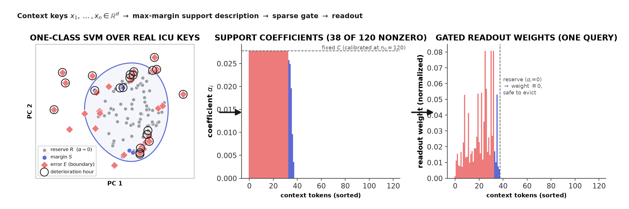
3.2 Exact fp64 increments and decrements↩︎
For certificate experiments we compute \(\alpha\) in fp64 with the maintained incremental algorithm of [11] (the same exact add/remove machinery was developed for support vector regression by [27]), which we ported and verified (Section 7). The solver receives \(C\) directly and keeps it unchanged for its lifetime. It adds one key at a time, raising its coefficient adiabatically while preserving the KKT conditions of all previous keys, with set migrations handled by rank-one updates of \(\mathcal{R} = M^{-1}\), the inverse of the bordered KKT matrix \[M = \begin{bmatrix} 0 & \mathbf{1}^\top \\ \mathbf{1} & 2K_{SS} \end{bmatrix},\] where \(K_{SS}\) is the Gram matrix restricted to the margin set. With \(C\) held fixed, the procedure is reversible: driving a coefficient back to zero along the same path removes the key exactly, returning the solver to the state it would occupy had the key never entered under the same algorithm and hyperparameters. In our fp64 verification suite a decrement composed with the increment that preceded it restored the solution to within \({\sim}10^{-16}\) on well-conditioned data. All exact-deletion claims use this path, not the batched training approximation below.
3.3 The inverse-reusing custom backward↩︎
For the exact maintained path, within a fixed partition the free variables \(u = [\rho;\, \alpha_S]\) satisfy \(Mu = c\), where \(\rho\) is the multiplier
of the equality constraint and \(c\) collects the constant terms contributed by \(E\). By the implicit function theorem, a custom vector–Jacobian product for an upstream cotangent \(\bar u\) reuses \(\mathcal{R}\): with \(w = \mathcal{R}^\top \bar u\), the gradient \(\partial L/\partial K\) is a sum of
rank-one outer products of \(w\) and \(\alpha_S\) (full expressions in Appendix 12). Because the forward pass already maintains \(\mathcal{R}\), this custom backward performs no second system solve. Set migrations are measure-zero, piecewise-smooth boundaries, which we treat as ReLU-style kinks and do not differentiate through. The expressions match
finite differences under double-precision gradcheck (Section 7). This no-second-solve statement does not apply to the batched path.
3.4 A stabilized batched training path↩︎
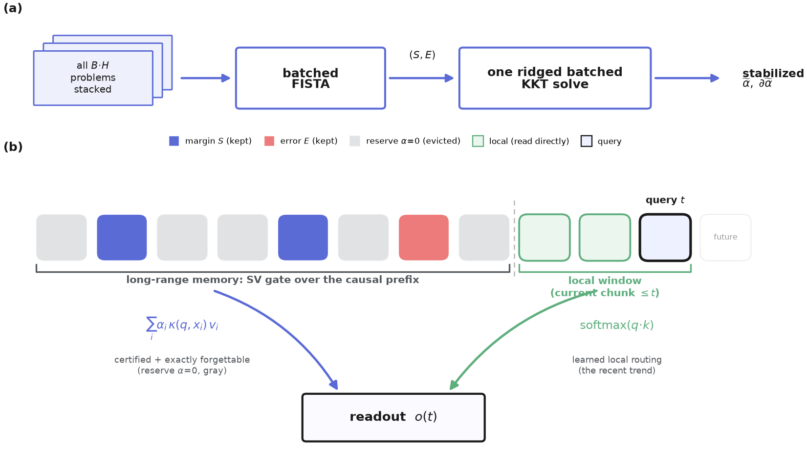
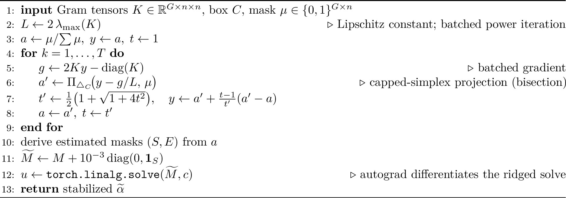
Solved per (sequence, head) and, in the causal layer, per chunk boundary, a sequential active-set walk in Python does not use the GPU and is the layer’s throughput bottleneck. We therefore use a separate, stabilized approximation for training (Figure 2a). First, a single batched accelerated projected-gradient solver (FISTA, [28]) estimates the partition for all problems
at once: 1 is a box- and sum-constrained convex quadratic program, so each iteration is a dense batched matrix product plus a vectorized capped-simplex projection, fused into one compiled graph and masked so problems of different
prefix length pack into one batch (Algorithm 7, Appendix 13). We run this partition finder in single precision on Apple-silicon GPUs through MLX [29]. Second, the PyTorch path constructs the bordered KKT system for those masks, adds a ridge of \(10^{-3}\) to the margin block, and calls torch.linalg.solve;
standard autograd differentiates that solve. We denote the resulting coefficients \(\widetilde{\alpha}\). The ridge stabilizes redundant-key batches, but it also means \(\widetilde{\alpha}\)
is an approximation to the coefficients of 1 . This path neither uses the inverse-reusing custom VJP nor supplies an exact-deletion certificate. Its throughput consequence is in Section 7.0.0.2.
3.5 A causal layer and a local path↩︎
We lift the block gate to a causal, multi-head sequence layer with a chunk-frozen update (Titans-MAC style): the sequence is processed in chunks, and queries in a chunk read against the gate state fit on the causal prefix. Under exact inference, each boundary admits the new keys to the fixed-\(C\) maintained solver and may evict certified-inert reserve tokens; batched training instead recomputes the approximate partition. Within a fixed estimated partition the per-chunk readout is differentiable through the ridged batched solve and autograd, so the layer trains end-to-end; the gate state is detached across chunk boundaries (a chunk-frozen approximation controlled by the chunk length), which costs \(0.04\%\) bits-per-character against a token-level update ablation at small scale.
Trained as a pure chunk-frozen gate the layer plateaus as a language-model layer. We localize the cause by ablation (Section 8): it is neither the kernel nor the gate but the chunk-frozen contract itself, which makes a query read the gate fit on the prefix before its chunk and therefore never see the most recent tokens, the local context that dominates next-token prediction. We add a local path (Figure 2b): a query at position \(t\) attends, with a learned \(q\!\cdot\!k\) softmax, over all of \([0, t]\), where the chunk-frozen long-range prefix is weighted by the gate coefficient and the recent tokens inside its own chunk are read directly. This is a gated-global, dense-local pattern in the spirit of long-context sparse attention [22]; it preserves causality and differentiability (verified by gradient check).
3.5.0.1 Hybrid deletion semantics.
The support-vector certificate applies to the long-range prefix when it is solved by the exact fixed-\(C\) maintained solver: deleting an admitted token follows the decremental reverse path and re-solves the remaining gate. A token in the current chunk has not yet been admitted to that gate. Deleting it masks its raw key/value slot and its attention weight, then renormalizes the remaining weights; the mask also excludes it at future admissions. This is direct local-cache deletion, not a support-vector certificate. During training, the long-range gate uses the stabilized batched approximation while the local path remains dense; exact deletion is certified only when the long-range gate is recomputed by the fp64 maintained path.
4 Exact forgetting↩︎
We test exact forgetting twice: first as a concrete, legible removal, then against the formal definition of exact unlearning. Every deletion and selection certificate in this and the next two sections uses the maintained CPU solver in fp64. For trained-model experiments, the model supplies frozen learned keys, which are then solved and deleted with that fp64 path. Language-model training and the throughput benchmark use the stabilized batched path and are not used to certify exact deletion.
4.0.0.1 Removing a planted secret.
We add a distinctive (key, value) pair to \(14\) ordinary context tokens (\(d=4\), \(\sigma=1.5\)), giving admission size \(n_0=15\). The reporting parameter \(\nu=0.5\) calibrates \(C=1/(\nu n_0)=2/15\) once, and that \(C\) is held fixed for deletion and the never-saw-it reference. We probe near every key over \(30\) trials. Before forgetting, a probe near the secret retrieved it in \(80\%\) of trials. The exact decrement left a maximum readout deviation of \(8.9\times10^{-5}\) from a layer that never contained the secret, and the secret was retrieved in \(0\%\) of trials. Decay-style forgetting (scaling the secret’s coefficient by \(\gamma\)) left deviations of \(0.57\), \(0.34\), and \(0.16\) at \(\gamma = 0.5, 0.1, 0.01\), and still surfaced the secret in \(80\%\), \(40\%\), and \(7\%\) of trials. Even a \(99\%\) decay leaves the layer measurably shaped by the token; the decremental path removes the shape itself, because the remaining coefficients are re-solved to the optimum they would have reached without it.
4.0.0.2 Equivalence to retraining.
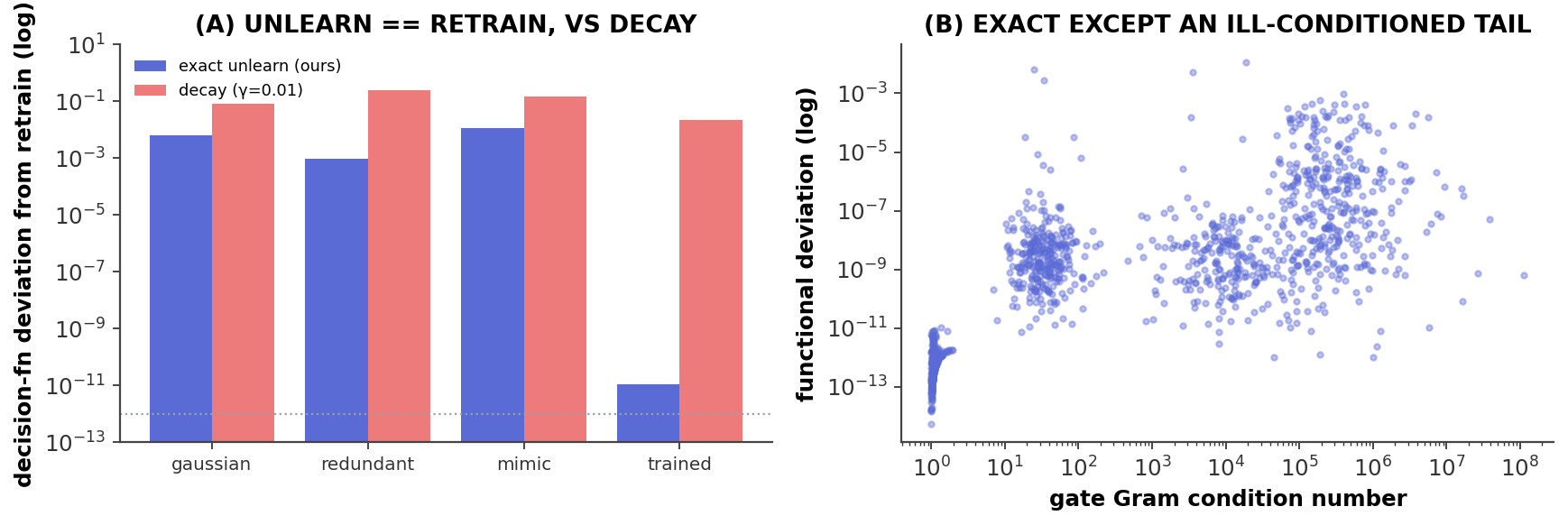
Exact (“perfect”) unlearning is defined as equivalence to retraining from scratch without the data [9], [12]. That reference must use the same learning algorithm and hyperparameters. Here \(C\) is the primitive hyperparameter: decrement and retrain-without both retain the \(C\) calibrated at \(n_0\). Replacing it by \(1/(\nu(n_0-1))\) after one deletion would change the optimization problem and would not be a same-algorithm unlearning test. We evaluate the fixed-\(C\) decrement on two levels. State-level. Where the SVDD optimum is unique, the decremental reverse path recovers the same active-set partition \((S,E,R)\) and coefficients \(\alpha\), up to fp64 numerical tolerance, as a from-scratch refit on the retained tokens. The observed partition-match rates are \(99\%\), \(98\%\), and \(100\%\) on Gaussian, real MIMIC-IV, and trained-model keys respectively (Table 1). On exact duplicates the optimum is non-unique, so \(\alpha\) and the partition can legitimately differ (\(52\%\) match) without any forgetting failure, which is why we also measure at the function level. Function-level (the duplicate-invariant metric). We compare the decision functions \(f(x) = 2\sum_i \alpha_i \kappa(x, x_i) - \rho\) of the decrement and the refit on probes spanning the retained, forgotten, and jittered points, over \(300\) trials per regime. The deviation has a median of \(4.5\times10^{-13}\) on the trained model’s learned keys and \({\sim}10^{-9}\) on well-conditioned Gaussian and real-ICU keys, rising to a worst case of \(1.1\times10^{-2}\) confined to the ill-conditioned near-duplicate tail, which deduplication removes (Figure 3b); the mean is pulled up by that tail, so the median is the representative figure. Coefficient decay, on the identical metric, deviates by \(2.2\times10^{-2}\) to \(2.4\times10^{-1}\) (median), larger than our worst case in every regime and five to eleven orders of magnitude larger at the median, because it never re-solves and its gate still reflects the forgotten token. The precise boundary of the claim is therefore algorithmic equivalence to the same fixed-\(C\) retrain-without problem, realized numerically in fp64 and reported with the measured function deviations above. The threat model is decision/readout influence, not membership inference.
4.0.0.3 The cost of a deletion.
The decrement is also cheap: an active-token removal uses rank-one updates on the maintained KKT inverse, while a certified-inert reserve token deletes directly. In our deterministic benchmark, a uniformly selected deletion completes in \(0.31\)–\(1.23\) ms on an Apple M3 Ultra CPU for contexts of \(120\)–\(512\) tokens (the regime of our ICU streams), \(18\)–\(197\times\) faster than a from-scratch retained-set QP refit with the same primitive box \(C\) held fixed (median over \(30\) trials per context length; experiments/deletion_latency.py). Across all trials, the maximum decision-function deviation from that refit was \(5.3\times10^{-4}\).
| regime | partition match | decrement f-dev (median / mean / worst) | decay f-dev (median) |
|---|---|---|---|
| Gaussian (distinct) | \(99\%\) | \(2.4\mathrm{e}{-}9\) / \(3.1\mathrm{e}{-}5\) / \(6.4\mathrm{e}{-}3\) | \(8.3\mathrm{e}{-}2\) |
| redundant (duplicates) | \(52\%\) | \(5.7\mathrm{e}{-}7\) / \(3.1\mathrm{e}{-}5\) / \(9.6\mathrm{e}{-}4\) | \(2.4\mathrm{e}{-}1\) |
| MIMIC-IV (real ICU) | \(98\%\) | \(1.6\mathrm{e}{-}9\) / \(5.6\mathrm{e}{-}5\) / \(1.1\mathrm{e}{-}2\) | \(1.5\mathrm{e}{-}1\) |
| trained model keys | \(\mathbf{100\%}\) | \(\mathbf{4.5\mathrm{e}{-}13}\) / \(9.7\mathrm{e}{-}13\) / \(1.1\mathrm{e}{-}11\) | \(2.2\mathrm{e}{-}2\) |
5 Certified selection↩︎
Certified selection is the second property the active-set partition confers: because reserve tokens are provably inert, evicting them to a bounded budget cannot change the output. We establish it on the smallest tasks that can falsify it, against the eviction baselines (H2O-style heavy hitters, recency, random) and the efficient-attention baselines (linear attention, DeltaNet) a deployed selector must beat.
5.0.0.1 The gate earns its keep under redundancy.
A control experiment first scopes where the gate does and does not help. On a causal multi-query associative-recall sweep [30] over distinct keys (Table 2), the distance-kernel readout holds recall@1 at \(0.96\)–\(0.99\) while softmax decays from \(0.87\) to \(0.14\) and the matched-state inner-product recurrences (DeltaNet, linear) collapse to chance: the distance kernel retrieves where dot-product memories cannot. But a gate-off ablation (uniform weights, same readout) matches the gate on distinct keys and slightly exceeds it at the highest load (\(0.99\) vs.\(0.88\) at \(64\) items): on clean, non-redundant keys the max-margin gate can drop a still-needed key for no benefit. The advantage there is the distance kernel, not the gate. The gate earns its keep under redundancy, which the next results isolate.
| # distinct items | softmax | DeltaNet | linear | SV (no gate) | SV-Attn |
|---|---|---|---|---|---|
| 4 | 0.870 | 0.295 | 0.422 | 0.965 | 0.979 |
| 8 | 0.779 | 0.140 | 0.202 | 0.980 | 0.985 |
| 16 | 0.692 | 0.077 | 0.077 | 0.982 | 0.976 |
| 32 | 0.411 | 0.029 | 0.032 | 0.984 | 0.976 |
| 64 | 0.144 | 0.017 | 0.017 | 0.987 | 0.875 |
5.0.0.2 The gate is load-bearing on selective copying.
The selective-copying task [6] is the opposite regime: a handful of informative (content, value) tokens must be recovered from a growing field of near-duplicate zero-value filler. With \(8\) informative tokens and \(F\) filler tokens (Table 3), SV-Attention holds recall@1 at \({\sim}0.99\) as \(F\) grows from \(8\) to \(120\), while softmax is diluted to \(0.48\)–\(0.76\) and the fixed-state recurrences fade. The mechanism is the certified reserve: the support set stays at \(11\)–\(14\) tokens regardless of length, so the working state does not grow with the distractor mass.
| filler \(F\) (length \(L\)) | SV-Attn | softmax | DeltaNet | linear | SV state |
|---|---|---|---|---|---|
| \(8\) (\(16\)) | 0.990 | 0.707 | 0.353 | 0.153 | 11.6 |
| \(24\) (\(32\)) | 0.993 | 0.477 | 0.310 | 0.180 | 11.0 |
| \(56\) (\(64\)) | 0.990 | 0.757 | 0.290 | 0.167 | 11.1 |
| \(120\) (\(128\)) | 0.993 | 0.693 | 0.230 | 0.183 | 14.0 |
5.0.0.3 Matched-budget selection beats heavy-hitter eviction.
We construct contexts with skewed redundancy: \(6\) rare groups of one key each and \(6\) dense groups of \(10\) near-duplicate keys (\(n = 66\) tokens, \(12\) effective items); two queries probe each group. We fix a token budget equal to the gate’s support size and compare selection policies with an identical uniform-RBF readout, so only the selection differs: the certified support set; an H2O-style policy keeping the top-\(k\) tokens by accumulated attention mass [7], given an oracle form (scoring with the evaluation queries) and a warm form (scoring with an early half, then serving unseen queries); recency; and random. Over \(60\) trials at a \({\sim}56\%\) budget (Table 4), the certified gate beats every baseline; the gap is starkest on rare items (\(0.86\) vs.\(0.32\) for H2O), because under redundancy the heavy hitters are the duplicated keys. The gate also exceeds full-context recall (\(0.93\) vs.\(0.86\)), as evicting certified-inert duplicates removes mass that crowds rare keys out of the kernel sum, and the advantage grows as the budget tightens: at a \(41\%\) budget, rare-item recall is \(0.94\) (gate) vs.\(0.21\) (H2O). Streaming a redundant context through the causal layer with an online bounded budget (deciding eviction before future queries are known), certified selection retains rare items at \(0.93\) versus \(0.30\) for streaming heavy-hitter eviction, confirming the result survives causal operation.
| policy | recall, all groups | recall, rare groups |
|---|---|---|
| SV gate (certified, query-independent) | 0.929 | 0.861 |
| H2O heavy-hitter (oracle queries) | 0.571 | 0.319 |
| H2O heavy-hitter (warm/streaming) | 0.571 | 0.317 |
| recency-\(k\) | 0.336 | 0.000 |
| random-\(k\) | 0.733 | 0.472 |
| full context (no eviction) | 0.861 | 0.722 |
5.0.0.4 An adaptive bounded state outlasts a fixed-state recurrence.
A fair capacity comparison against DeltaNet must isolate state capacity from the similarity function, since the distance kernel retrieves on non-orthogonal keys where inner-product memories cannot. We therefore use near-orthogonal content keys, on which every method retrieves perfectly at low load, and grow the number of distinct items at a fixed block of \(20\) filler tokens (Table 5). All methods ace \(8\) items (confirming fairness), then the fixed-state baselines fade as distinct items exceed capacity (DeltaNet \(0.93\!\to\!0.06\)), while SV-Attention holds near \(1.0\) through \(24\) items and \(0.95\) at \(40\), its support set growing adaptively (\(9\!\to\!37\)) but well below full context. DeltaNet’s capacity scales with its state dimension, so this is a matched-state claim, not an absolute one.
| # distinct items | SV-Attn | softmax (full) | DeltaNet | linear | SV state |
|---|---|---|---|---|---|
| 8 | 1.000 | 1.000 | 1.000 | 1.000 | 9 |
| 16 | 1.000 | 1.000 | 0.930 | 0.250 | 16 |
| 24 | 1.000 | 0.857 | 0.317 | 0.077 | 23 |
| 40 | 0.947 | 0.783 | 0.060 | 0.023 | 37 |
6 Capabilities on real data↩︎
We now demonstrate the two properties as concrete capabilities on a trained model, on real intensive-care records, and on real text, rather than as aggregate metrics alone. In each case, the certificate is computed by the exact fixed-\(C\) fp64 solver.
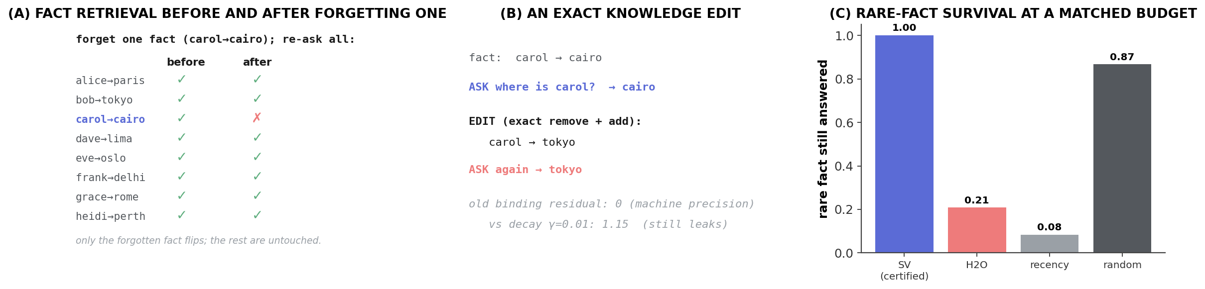
6.0.0.1 Surgical forgetting and exact editing on a trained model
(Figure 4). We freeze the learned keys of a trained multi-query associative-recall model [30] (recall@1 \(= 1.0\)) and pass them to the fp64 maintained solver. Forgetting one fact drops its retrieval from \(1.0\) to chance while every other fact remains perfectly answerable: the unlearning is targeted, with no collateral damage. An exact fixed-\(C\) remove-and-add edits a fact (“carol \(\to\) cairo” becomes “carol \(\to\) tokyo”); the old binding’s residual influence is \(0\) to machine precision, versus \(1.15\) for decay. Under redundancy, certified eviction keeps a queried rare fact \(100\%\) of the time at a token budget where heavy-hitter (H2O) eviction keeps it \(21\%\).
6.0.0.2 Right-to-be-forgotten and certified retention on real ICU streams
(Figure 5). Intensive-care vital-sign records are a near-ideal stress test: a patient is monitored for days, most hours are physiologically stable and nearly identical to their neighbors, and the decisive moments are rare and irregular. We built hourly token streams from the MIMIC-IV v3.1 ICU module [13]: \(1{,}465\) stays of at least \(48\) hours, six routine vitals binned to hourly means, forward-filled and standardized, a Harutyunyan-style feature set [31]. Solving the gate per stay, the certified-inert reserve fraction is \(0.667\) and stable with length: roughly two of every three monitored hours are provably redundant. At a matched budget equal to the support-set size (mean \(33\%\) of the stream), with an identical uniform-RBF readout, the certified gate retained \(0.80\) of the rare deterioration hours a clinician must not lose, against \(0.05\) for heavy-hitter eviction (Table 6); deterioration hours are physiologic outliers, and the one-class support set is outlier-aware by construction, whereas heavy-hitter mass concentrates on the dense, stable hours. Separately, fixed-\(C\) fp64 decremental forgetting of one of several patients sharing a context removed only that patient (no longer retrievable; the others untouched and the retained state an exact solution, KKT residual \({\sim}10^{-12}\)), and the forgotten patient’s record leaked zero weight into the readout, against \(0.29\) and \(0.09\) under decay: a right-to-be-forgotten deletion with a numerical certificate, on real records.
| policy | deterioration-hour retention | deterioration-hour retrieval |
|---|---|---|
| SV gate (certified, query-independent) | 0.80 | 0.95 |
| H2O heavy-hitter | 0.05 | 0.13 |
| recency-\(k\) | 0.30 | 0.45 |
| random-\(k\) | 0.34 | 0.61 |

6.0.0.3 Downstream prediction is competitive.
Beyond selection, we ask the head-to-head question directly: at each hour, predict whether any vital crosses a deterioration threshold within the next six hours, a future-outcome task, so the label and the gate do not read the same hour’s vitals. Training the causal SV-Attention layer and the sequence baselines (Table 7), SV-Attention is competitive but not best: AUROC \(0.70\) versus \(0.78\) for an LSTM and \(0.75\) for softmax. A \(2\times2\) ablation crossing the gate update (chunk-frozen vs.per-token) with the selection mechanism (max-margin gate vs.uniform-RBF readout) localizes the gap: a uniform-RBF readout with per-token updates matches softmax (\(0.751\)), while the chunk-frozen blind spot (a query misses the most recent hours) and the max-margin selection (weight on atypical rather than recently-trending tokens) each cap AUROC near \(0.70\) and are partly redundant. The selection that wins certified retention is the same selection that mildly costs prediction, here \({\sim}0.05\) AUROC.
| model | AUROC | AUPRC |
|---|---|---|
| LSTM | 0.783 | 0.709 |
| softmax | 0.751 | 0.664 |
| DeltaNet | 0.746 | 0.665 |
| linear | 0.746 | 0.660 |
| SV-Attention | 0.696 | 0.598 |
6.0.0.4 A certified, forgettable retrieval memory over real text
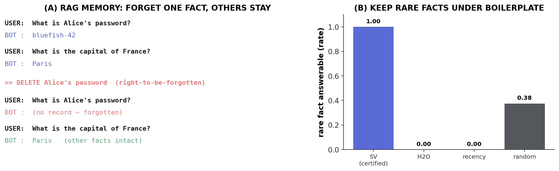
(Figure 6). We build a retrieval memory whose fact keys are real MiniLM sentence embeddings and whose gate is the exact fixed-\(C\) fp64 one-class SVM; it answers \(7/7\) natural-language questions. Deleting “Alice’s password” makes the system return “no record—forgotten” on that query while other facts answer unchanged, and under boilerplate redundancy certified eviction keeps a rare fact answerable (\(1.00\)) where heavy-hitter eviction does not (\(0.00\)). This is the deployable framing: a retrieval-augmented memory [32] for a language model whose retention and deletion are auditable rather than scored.
7 The gate is correct and trainable↩︎
7.0.0.1 Maintained-solver and gradient verification.
We verify the exact path’s custom implicit backward with double-precision gradcheck (\(\epsilon = 10^{-6}\)), differentiating through the kernel map so perturbations preserve the symmetry of \(K\) and the partition is locally stable; gradcheck passes for a scalarization of \((\alpha,\rho)\), for the decision scores, and for the full layer readout \(o(q)\) with respect to keys, values, and queries. A student layer trained by Adam to match a teacher SV-Attention mapping reduced loss by \(99\%\) in \(200\)
steps, confirming that custom-VJP gradients are usable, not merely correct. We separately gradcheck the batched torch.linalg.solve/autograd path end to end; that check validates the derivative of the ridged approximation, not exact
coefficients of 1 . We verified the maintained incremental solver against an independent interior-point QP: on well-conditioned data it matched the batch optimum at every point of a \(45\)-point
stream (worst decision-value gap \(1.6\times10^{-6}\)), removal matched the batch optimum on the retained set (\(2.7\times10^{-7}\)), and decrement\(\circ\)increment restored the state to \(4.4\times10^{-16}\). On near-duplicate points the key Gram matrix can reach condition number \({\sim}10^{11}\) and the
optimum is effectively non-unique, so fixed-\(C\) retraining equivalence is reported at the decision-function level with a logged numerical tolerance.
7.0.0.2 The batched solver makes the gate trainable at scale.
Table 8 times a full forward/backward step at the \(3.22\)M configuration (four layers, \(d_{\text{model}}{=}256\), block \(256\), batch \(16\)). Each direct row is the median of seven synchronized repetitions after three warm-ups. The current hybrid path spans PyTorch on CPU (model, ridged KKT solve, and autograd) and MLX on the Apple GPU (FISTA partition finder), including transfers between them. It reaches \(9{,}125\) tokens/s: \(6.11\times\) the step time of an unfused PyTorch CPU softmax reference and \(35.80\times\) the step time of the corresponding MPS reference. The two exact active-set rows are historical RBF-only diagnostics, measured directly at batch \(2\) and linearly extrapolated to batch \(16\); they are not like-for-like hybrid measurements. A \(50\)k-step projection for the directly measured mixed path is \(6.23\) hours, excluding optimizer updates, data loading, evaluation, and checkpoints. The \(10\)M model we study (Section 8; \(d_{\text{model}}{=}384\), block \(512\)) runs at \({\sim}2{,}400\) tokens/s and trains for \(6{,}000\) steps in under six hours. The comparison establishes practical small-scale training, not throughput parity; a fused softmax kernel would widen the accelerator gap.
| method | device / measurement | ms/step | tokens/s | rel.time |
|---|---|---|---|---|
| softmax reference | PyTorch CPU, direct | \(73.4\) | \(55{,}789\) | \(1.00\times\) |
| softmax reference | PyTorch MPS, direct | \(12.5\) | \(326{,}648\) | \(0.17\times\) |
| SV exact re-stream RBF\(^\ast\) | CPU, extrapolated | \(17{,}336\) | \(236\) | \(236.12\times\) |
| SV exact persistent RBF\(^\ast\) | CPU, extrapolated | \(10{,}538\) | \(389\) | \(143.53\times\) |
| SV hybrid, batched | PyTorch CPU + MLX GPU, direct | \(\mathbf{448.9}\) | \(\mathbf{9{,}125}\) | \(\mathbf{6.11\times}\) |
8 A language-model usability probe↩︎
This section asks whether the hybrid layer is a usable sequence layer at a matched token budget. We use byte-level corpora with no tokenizer, where a controlled comparison is cleanest, and report on both standard enwik8 and the contemporary TinyStories corpus [33] at two model scales. The only fair state-matched comparison is against a sliding-window softmax Transformer (“Transformer++,” swa), whose window we set to the hybrid’s measured state; recurrent baselines (DeltaNet, linear) carry their own state and are reported at it (full protocol in Appendix 14).
At \(3.22\)M parameters (Table 9), the seven-seed mean BPC is \(2.178\) for the hybrid and \(2.383\) for the matched-state Transformer++. Every paired seed favors the hybrid, with a mean relative improvement of \(8.6\%\) (\(95\%\) CI \([5.2,12.0]\%\); paired \(t=5.95\), two-sided \(p=0.001\); Appendix 15). The DeltaNet, linear-attention, and full-softmax entries are single-seed reference runs, so we do not use them for multi-seed inference; they suggest that DeltaNet, with its larger matrix state, is the stronger raw predictor. On TinyStories, all three paired seeds favor the hybrid by \(14.2\%\) on average, but this is a directional replication at \(n=3\), not a statistically confirmed result (\(p=0.057\)). The hybrid’s distinction is the certifiable exact-solver memory that the recurrences cannot provide, not dominance in raw perplexity.
The small-scale edge does not extend to larger models. Repeating the matched-state comparison at \(10\)M parameters (block \(512\), five seeds) is a wash: SV is \(2.5\%\) worse than swa on average with very high seed variance (sd \({\sim}15\%\); not significant), and a single \(32\)M run is similar. Two effects compound. At block \(512\) the matched window is most of the context, so the sliding-window baseline is already near-full attention and leaves little for a selective long-range memory to win. More importantly, the chunk-frozen gate optimizes more slowly and less stably at scale: several \(10\)M seeds (and the \(32\)M run) had not converged within our \(6{,}000\)-step budget (their loss was still descending), so the fixed-budget comparison penalizes them. We therefore scope the language-model edge to the small-scale regime and treat scalable, stable optimization of the gate as an open problem. This is a limitation of the language-modeling use; certified selection and exact deletion are properties of the separate fp64 maintained solve, established on real data and independent of language-model scale.
| layer | BPC | aggregation | state |
|---|---|---|---|
| DeltaNet | \(1.961\) | single seed | \(d_k{\times}d_v\) matrix |
| SV hybrid (ours) | \(\mathbf{2.178}\) | seven-seed mean | gated long-range \(+\) local |
| linear attention | \(2.215\) | single seed | \(d\)-dim |
| Transformer++ (sliding window, matched) | \(2.383\) | seven-seed mean | window (matched) |
| softmax (full attention) | \(2.359\) | single seed | full context |
9 Discussion↩︎
The experiments support a single thesis: when the inner problem of a test-time-learning layer is constrained and max-margin rather than dense and least-squares, the layer acquires structure that can be certified rather than merely measured. For the exact fixed-\(C\) solve, the active-set partition is not a score to be thresholded; it is a statement, backed by complementary slackness, about which tokens the readout provably ignores. This is the right lens on the empirical results. Heavy-hitter eviction lost on rare items not because its scoring is poorly tuned but because accumulated attention mass is a popularity statistic: under redundancy, popularity concentrates on duplicates, and the rare singletons that carry the information are exactly what gets evicted. The one-class gate inverts this failure mode by construction, spending its budget on the boundary of the key distribution, and the MIMIC-IV result is the same mechanism on data we did not design: deterioration hours are physiologic outliers, so a gate that keeps outliers keeps them, at a \(0.80\) vs.\(0.05\) retention gap.
Exactness of forgetting deserves a separate comment, because its value is regulatory as much as technical. Every gradient-based memory forgets by decay, which leaves behind an influence one can only bound empirically and argue about; the fp64 decremental path instead returns the solver to the state it would hold without the token under the same fixed \(C\), to a tolerance we log. We checked this not against a convenient probe but against the formal definition of exact unlearning, equivalence to same-algorithm retraining, on real ICU records and on a trained model’s own keys, and we measured coefficient decay on the identical yardstick so the gap is not an artifact of metric choice. When deleting a record is a legal or clinical obligation, “the residual was small” and “the model was provably re-solved without it” are not the same statement, and only the second is one an auditor can act on. This also marks where the layer does not help: the certificate is a statement about redundancy and atypicality, and a context with neither gives the gate nothing to certify, so it falls back to ordinary kernel attention. Fortunately the workloads that motivate long-context memory (boilerplate documents, vitals stable for hours, dialogue that repeats) are redundant in precisely this sense. In the hybrid, this certificate stops at the long-range gate: current-chunk tokens belong to the dense local path and are removed by masking and renormalization.
10 Limitations↩︎
The advantage is regime-specific. The selection advantage requires the informative tokens to be distributional outliers, or the context to be redundant; the gate is a one-class anomaly detector and confers no benefit where importance does not coincide with atypicality. It is an active-set solve, not a fused kernel. The current mixed CPU–MLX implementation is \(6.1\times\) slower than an unfused CPU softmax reference and \(35.8\times\) slower than its MPS reference, so it is not a throughput-competitive general-purpose attention layer.
The language-model edge is confined to small scale. The significant enwik8 matched-state win (\(8.6\%\), \(p=0.001\), seven seeds) is at \(3.22\)M parameters. TinyStories is a three-seed directional replication (\(14.2\%\) mean improvement, \(p=0.057\)), not statistical confirmation. At \(10\)M (five seeds) the comparison is a wash and a \(32\)M run is similar. The chunk-frozen gate converges markedly slower and less stably than softmax at \(10\)M–\(32\)M; a stable, budget-efficient optimizer for the gate at scale is an open problem we do not solve here. This is the central obstacle to the language-modeling use; it does not affect the exact-solver certificate experiments.
The training path is approximate and the hybrid certificate is long-range only. Batched training uses an estimated partition, a \(10^{-3}\) ridge,
torch.linalg.solve, and autograd. It does not produce exact SVDD coefficients, does not reuse a maintained inverse in backward, and carries no exact-deletion certificate. Exact deletion requires the fixed-\(C\) fp64 maintained solver. Within the hybrid, that certificate covers admitted long-range tokens; deleting a current-chunk local token masks its raw slot/weight and renormalizes, with no SV certificate.Exactness carries a logged tolerance on ill-conditioned streams. Where the optimum is unique, the fixed-\(C\) decrement and retrain-without target the same state; in fp64 we report the observed partition match and function deviation. On near-duplicate keys the optimum is non-unique and conditioning degrades, with a logged worst-case decision-function deviation of \(1.1\times10^{-2}\); deduplication is required on maximally redundant streams. We also found one edge case (the margin set emptying mid-decrement) unhandled in both our solver and the reference, which deduplication avoids but a production decrement path should cover. Finally, fixed-\(C\) feasibility requires \(nC\geq1\) after deletion; below the implementation’s \(\lceil1/C\rceil+2\) admission threshold it falls back to the ungated path and makes no SV certificate.
Forgetting threat model. We measure decision/readout influence, not membership inference; deploying for compliance would require a privacy evaluation appropriate to the regulation.
The contribution is scale-independent. Certified selection and exact deletion are properties of the fixed-\(C\) fp64 solve, established on real MIMIC-IV records and a trained model’s learned representations; they do not depend on language-model scale, so the small-scale probe caveat above does not weaken those solver-level results.
11 Conclusion↩︎
We added the constrained, max-margin member to the test-time-learning family of attention layers. Its exact fixed-\(C\) fp64 maintained solver provides certified selection, exact forgetting relative to same-algorithm
retraining, and a custom backward that reuses the forward-maintained KKT inverse. A separate \(10^{-3}\)-ridged batched torch.linalg.solve/autograd path makes training practical, but its coefficients are
approximate and it does not inherit the exact-deletion certificate. We verified the solver-level properties on real clinical streams and learned representations and made the hybrid boundary explicit: the certificate covers the long-range gate, while a
current-chunk deletion masks and renormalizes the local path. As attention systems take on longer contexts and stricter retention obligations, such precisely scoped guarantees can be evaluated alongside predictive and throughput benchmarks.
Broader Impact↩︎
Exact, auditable deletion of a token’s influence is a capability with an obvious upside for deployed systems that must honor erasure requests: a mechanism whose removals can be demonstrated is preferable to one whose removals can only be claimed. We are deliberate about its limits. The guarantee applies to the exact fixed-\(C\) fp64 long-range gate, not the ridged batched training path or the hybrid’s local-path mask. It concerns decision and readout behavior, not membership inference, so a deleted long-range token is “forgotten” in the sense that the memory’s outputs match a same-hyperparameter model that never held it, not in the sense of a formal privacy bound; a compliance use would need to be paired with a privacy evaluation matched to the relevant regulation. The clinical study is retrospective on de-identified MIMIC-IV data used under its credentialed agreement, the deterioration labels are alarm thresholds rather than validated endpoints, and none of this constitutes a clinical tool absent prospective validation.
Data Availability and Reproducibility↩︎
The clinical experiments use the MIMIC-IV v3.1 ICU module [13], a de-identified record dataset released by the MIT Laboratory for Computational Physiology through PhysioNet and available to credentialed researchers under the PhysioNet Credentialed Health Data Use Agreement; the data were used in accordance with that agreement. Because the agreement prohibits redistribution of the dataset or its derivatives, we release the full preprocessing and experiment code, which reproduces every clinical result from the raw PhysioNet files, but not the data or any derived caches. The verified solver, the batched GPU gate, the hybrid layer, the full verification suite, and every synthetic experiment and figure are released as code with fixed seeds. Source and reproducibility materials are available at https://github.com/vishrmsh/sv-attention.
12 The implicit vector–Jacobian product↩︎
This section describes the custom backward for the exact fp64 maintained solver; it is not the backward used by the stabilized batched training path. Within a fixed active-set partition \((S, E, R)\) the free variables
\(u = [\rho;\, \alpha_S]\) satisfy the bordered KKT system \(M u = c\), with \(M = [[0, \mathbf{1}^\top],[\mathbf{1},
2K_{SS}]]\) and \[c = \begin{bmatrix} 1 - |E|\,C \\ \mathrm{diag}(K)_S - 2C\, K_{SE}\mathbf{1} \end{bmatrix},
\qquad u = \mathcal{R} c, \quad \mathcal{R} = M^{-1}.\] For a loss \(L\) with upstream cotangents \(\bar\rho, \bar\alpha_S\), let \(\bar u = [\bar\rho;\,
\bar\alpha_S]\) and \(w = \mathcal{R}^\top \bar u\) with margin block \(w_S\). Differentiating \(u = \mathcal{R} c\) and using \(d\mathcal{R} = -\mathcal{R}\, dM\,
\mathcal{R}\) gives \(dL = w^\top dc - w^\top dM\, u\); collecting the coefficients of \(dK_{ij}\), \[\begin{align}
\frac{\partial L}{\partial K_{ii}} &\mathrel{+}= [w_S]_i && (i \in S), &
\frac{\partial L}{\partial K_{ie}} &\mathrel{+}= -2C\,[w_S]_i && (i \in S,\, e \in E), &
\frac{\partial L}{\partial K_{ij}} &\mathrel{+}= -2\,[w_S]_i\,[\alpha_S]_j && (i, j \in S).
\end{align}\] Every term is a rank-one assembly, and the custom backward only multiplies by \(\mathcal{R}^\top\), which the exact forward pass already maintains; it performs no second system solve. Changes in the
active set happen on a measure-zero set of inputs across which the map is piecewise smooth; as with the kink in a ReLU, we do not route gradient through the discrete change in set membership. The expressions are verified against finite differences by
double-precision gradcheck. This inverse-reuse/no-second-solve statement does not apply to Appendix 13.
13 The batched projected-gradient solver↩︎
The language-model training forward uses a stabilized approximation for every (sequence, head, chunk) problem. A sequential active-set walk solves one problem at a time; instead, the single-precision accelerated projected gradient of Algorithm 7 estimates all partitions at once. Because 1 is a box- and sum-constrained convex quadratic program, each FISTA step is a dense batched matrix product and a vectorized projection onto the capped simplex \(\{a : \sum_i a_i = 1,\, 0 \le a_i \le C\}\), computed by bisection on the dual variable. The projection and step are fused into one compiled graph and run through MLX [29]; a per-row mask lets problems of different prefix length share one batch.
The estimated coefficients define masks \((S,E)\). In PyTorch, the implementation packs their bordered KKT systems, adds a fixed ridge \(\lambda=10^{-3}\) to each valid margin diagonal,
and computes \[\widetilde{M}u=c,\qquad
\widetilde{M}=M+\lambda\,\mathrm{diag}(0,\mathbf{1}_S),
\qquad \widetilde{\alpha}_S=u_S\] with torch.linalg.solve. Standard autograd differentiates this solve. Thus \(\widetilde{\alpha}\) is the exact solution of the ridged packed system, but only a
stabilized approximation to the unregularized coefficients of 1 . This path neither invokes the custom VJP of Appendix 12 nor inherits its no-second-solve property, and it is not used for an
exact-deletion certificate.
14 Experimental details↩︎
14.0.0.1 Models and training.
The backbone is a pre-norm decoder with token and learned positional embeddings, a weight-tied output head, and a pluggable attention module so every variant shares an identical backbone. The \(3.22\)M configuration is \(d_{\text{model}}{=}256\), \(4\) layers, \(4\) heads, block \(256\); the \(10\)M configuration is \(d_{\text{model}}{=}384\), \(6\) layers, \(6\) heads, block \(512\). All variants train with AdamW (\(\beta = (0.9, 0.95)\), weight decay \(0.1\)), gradient clip \(1.0\), a cosine schedule, batch \(16\), on enwik8 bytes (vocabulary \(256\)); we report the best validation BPC over training. The primitive solver hyperparameter is the box \(C\). The language-model runs set \(C=0.25\) directly. In studies that report \(\nu\), we calibrate \(C:=1/(\nu n_0)\) once at the declared admission/reference size \(n_0\), record that scalar, and do not recompute it as the context size changes. Because the constrained problem requires \(nC\geq1\), the causal implementation uses an ungated warm-up below \(\lceil1/C\rceil+2\) available keys and issues no SV certificate there. The gate uses an RBF kernel, chunk length \(64\), and \(80\) FISTA iterations in the batched solver.
All selection and exact-forgetting certificates use the maintained CPU solver in fp64 with fixed \(C\). The language-model training and throughput paths use the single-precision batched partition finder followed by the
\(10^{-3}\)-ridged torch.linalg.solve/autograd path; their coefficients are a stabilized training approximation. When a certificate is reported on a trained model, its frozen learned keys are re-solved by the
fp64 maintained solver. Clinical experiments use MIMIC-IV under its credentialed data use agreement.
14.0.0.2 Throughput protocol.
We run python -m experiments.g1_throughput --paper on an Apple M3 Ultra (32 physical CPU cores, 512 GiB unified memory), macOS 26.5, Python 3.11.14, PyTorch 2.12.1, NumPy 2.4.6, and MLX 0.31.2. A timed step is zero_grad plus
full-model forward, cross-entropy, and backward; it excludes the optimizer update, data loading, evaluation, and checkpointing. Direct rows use batch \(16\) and report the median and interquartile range of seven separately
synchronized samples after three warm-ups. The mixed SV row includes PyTorch CPU work, host/device transfers, MLX-GPU FISTA, the ridged PyTorch KKT solve, and backward. The two exact active-set diagnostics implement the RBF readout, are measured at batch
\(2\), and are linearly extrapolated by \(8\times\); they are retained as historical diagnostics rather than like-for-like hybrid comparisons. Softmax is the repository’s unfused masked
implementation, not FlashAttention.
14.0.0.3 Matched-state protocol.
For each seed we train the SV hybrid, measure its mean active state \(|S \cup E|\) on held-out data, and set the sliding-window Transformer’s window to that state plus the local-window length, so the two layers see a matched token budget. The recurrent baselines (DeltaNet, linear attention) carry their own fixed state and are reported at it; full softmax is the unbounded reference. The seven-seed paired comparison is only SV versus matched swa; the DeltaNet, linear, and full-softmax rows are single-seed references. Every variant uses the identical backbone, optimizer, schedule, and training token budget.
14.0.0.4 Exact-forgetting protocol.
For each trial we build a context, calibrate or set \(C\) once, solve the gate in fp64, and forget a token two ways: (i) the Cauwenberghs–Poggio decremental reverse path, and (ii) a from-scratch refit on the retained tokens with that same \(C\) (the “retrain-without” reference). This is required by the same-algorithm definition: recomputing \(C\) from the smaller retained-set size would change a primitive hyperparameter. We compare their decision functions \(f(x) = 2\sum_i \alpha_i \kappa(x, x_i) - \rho\) on probes spanning the retained, forgotten, and jittered points, and report the maximum deviation. We use the decision function rather than the raw coefficients because on exact duplicates the SVDD optimum is non-unique (\(\alpha\) and the partition may differ while the function is identical), so the function is the correct equivalence test. The decay baseline scales the forgotten token’s coefficient by \(\gamma\) and is evaluated on the same metric. Regimes: Gaussian keys (\(d{=}6\)), redundant near-duplicate clusters, real MIMIC-IV hourly vitals (six Harutyunyan-style core vitals [31], deduplicated within \(0.1\) standardized units), and a trained recall model’s learned key projections; \(300\) trials each.
15 Per-seed matched-state results↩︎
Table 10 gives the per-seed bits-per-character for the SV hybrid and the matched-state sliding-window Transformer (swa) at \(3.22\)M parameters, the basis for the significance test in Section 8. Every one of the seven seeds favors the hybrid. Mean BPC is \(2.178\) for SV and \(2.383\) for swa; the mean paired relative improvement is \(8.6\%\) (\(95\%\) CI \([5.2, 12.0]\%\)), with a paired \(t\)-test \(t = 5.95\) (\(p = 0.001\)), a distribution-free Wilcoxon signed-rank \(p = 0.016\), and Cohen \(d_z = 2.25\).
| seed | 0 | 1 | 2 | 3 | 4 | 5 | 6 | mean |
|---|---|---|---|---|---|---|---|---|
| SV hybrid | 2.110 | 2.104 | 2.139 | 2.120 | 2.310 | 2.303 | 2.159 | 2.178 |
| Transformer++ (matched) | 2.287 | 2.297 | 2.469 | 2.415 | 2.389 | 2.420 | 2.405 | 2.383 |
| improvement (%) | 7.7 | 8.4 | 13.4 | 12.2 | 3.3 | 4.8 | 10.2 | 8.6 |
On the contemporary TinyStories corpus [33] (also \(3.22\)M, byte-level), the hybrid wins directionally on all three seeds: BPC \(1.329/1.185/1.269\) versus matched swa \(1.434/1.451/1.526\), a mean improvement of \(14.2\%\) (paired \(t=4.0\), \(p=0.057\) at \(n=3\)). This is a small directional replication on a second corpus, not statistical confirmation.
15.0.0.1 Larger scales.
At \(10\)M parameters (block \(512\), five seeds) the matched-state comparison does not favor the hybrid: per-seed SV vs.swa BPC is \(2.406/2.502\), \(2.249/2.661\), \(2.415/2.426\), \(2.475/2.286\), \(3.127/2.524\), a mean of \(+2.5\%\) (SV worse) with a standard deviation of \({\sim}15\%\) (not significant). The SV runs are themselves high-variance: the two worst seeds had not converged within the \(6{,}000\)-step budget (their loss was still descending steeply), so the comparison is partly a fixed-budget artifact rather than a clean quality verdict. A single \(32\)M run tells the same story: the SV-hybrid reached only \(4.456\) BPC and was still descending at step \(6{,}000\), versus a converged swa at \(3.106\). The chunk-frozen gate optimizes slower and less stably at scale, and we scope the language-model edge to the small-scale regime accordingly (Section 10).