Generalized Segmented GRAND for Guesswork Reduction in Turbo Product Decoding
July 13, 2026
Abstract
GRAND can efficiently decode any moderately redundant code with near ML performance via noise effect guessing. For binary linear codes, Rowshan and Yuan’s Segmented GRAND was the first to show that constrained guessing can reduce guesswork. Although powerful, their approach requires a specific parity-check matrix structure that limits the number of constraints that can be exploited as well as the class of applicable codes. Here we introduce GSegGRAND, a generalization of Segmented GRAND that circumvents its limitations. Built on a novel parity check structure and a transformation that maps codes into this structure, GSegGRAND efficiently incorporates up to \(\log_2(n)\) constraints for a wide range of codes, reducing guesswork by an additional \(75 \%\) over Segmented GRAND. To leverage that advantage for soft-output decoding, we derive an accurate SO equation for GSegGRAND by extending SOGRAND to incorporate constrained guessing. Applying this SO to turbo product decoding, GSegGRAND achieves up to \(88 \%\) guesswork reduction, making it a promising candidate for low-latency decoding in future communication systems.
GRAND, Segmented GRAND, constrained guessing, turbo product decoding, SOGRAND
1 Introduction↩︎
Guessing random additive noise decoding (GRAND) [2] is a decoding framework capable of decoding any code of moderate redundancy, including non-linear codes [3], while achieving near ML performance. A core component is a noise effect generator that produces noise effects in decreasing order of likelihood. For each query, GRAND inverts the noise effect from the hard-decision channel output and returns the resulting vector as soon as it is a valid codeword. This principle can be applied to various channel models, such as hard-decision [2], soft-decision [4], or correlated channels [5], [6]. GRAND’s practicality has been demonstrated through multiple taped out chips [7]–[11] and hardware syntheses, e.g. [12]–[17].
Recently, there has been increased interest in the reduction of GRAND’s guesswork, i.e., the number of noise effect queries until a codeword is found or decoding is abandoned. Existing work either targets special codes and applications [18], [19] or is applicable to general linear codes [20]–[28]. One strategy is to exploit the syndrome of each query during decoding, enabling [24] to correct an additional bit error and [22] to terminate decoding early. Another promising direction is constrained guessing. For a binary linear code with parity check matrix \(H\), GRAND searches for a noise effect \(z^n\) that satisfies a set of parity constraints \(H z^n = s^{n-k}\), induced by the syndrome \(s^{n-k}\) of the received hard-decision. Guesswork can therefore be reduced by restricting the guessing to noise effects that already fulfill a subset of such constraints, where each constraint reduces guesswork by up to a factor of \(2\) [27]. This creates the challenge of designing noise effect generators that can incorporate constraints efficiently while preserving an accurate guessing order.
Rowshan and Yuan’s proposed Segmented GRAND [20], [21], [27], which generates constrained queries efficiently using multiple noise effect generators, each operating on distinct segments of the codeword bits. That approach requires that the parity check matrix be in a class that can be transformed into a special structure where there exists a subset of rows such that each row has 1s in distinct, non-overlapping columns. If the parity check matrix can be transformed into that form, for each of these rows, the columns containing 1s then define an individual segment. In this case, segment parities correspond to syndrome values, allowing each noise effect generator to skip the generation and testing of noise effects of incorrect parity. While Segmented GRAND reduces guesswork efficiently, its guesswork reduction is limited by the number of rows that can be transformed into the specific structure. The transformation becomes more challenging as more constraints are extracted, and an efficient method for extracting numerous constraints for any given code is currently lacking.
In this paper, we propose GSegGRAND, which operates on a new parity check structure into which a wide range of parity check matrices can be easily transformed. This structure and transformation, which we term balanced tree structure and balanced tree transformation, preserves the codebook and facilitates the extraction of additional constraints. For all practical codes that we tested, we consistently extracted \(4\) constraints enabling a guesswork reduction by a factor of \(16\) over ORBGRAND without constrained guessing. To achieve this, we propose a novel noise effect generator tailored to this generalized structure. Unlike Segmented GRAND, whose segment parities are fixed, GSegGRAND works with segment parities that form a linear binary subspace induced by the balanced tree structure. This paper demonstrates how GSegGRAND can efficiently iterate through noise effects within this subspace.
An important recent development of GRAND is SOGRAND [29], which produces accurate SO and facilitates iterative decoding of TPC. TPCs enable the construction of long and powerful codes that, when decoded with SOGRAND, can outperform LDPC codes used in the 5G New Radio [29].
GRAND variants with constrained guessing, such as Segmented GRAND or GSegGRAND, have the potential to reduce guesswork during TPC decoding, an application that remains largely unexplored. However, constrained guessing requires a more nuanced SO calculation: Feng et al. found that, when using ORBGRAND with noise effect skipping for even-weight codes, conditioning the noise effect probabilities on their parity improves the SO quality [30]. As GSegGRAND exploits multiple constraints for skipping, a generalization of that correction is necessary.
In this paper, we propose a general framework to improve SOGRAND’s SO for any GRAND algorithm with constrained guessing and demonstrate it on GSegGRAND. Our simulation results highlight the importance of the improved SO calculation for turbo product decoding: with the conventional SO calculation, constrained guessing suffers from a high error floor above a BLER of × 10−1 for the \((32, 26)^2\) eBCH TPC. In contrast, with the proposed SO calculation, GSegGRAND reaches a BLER performance close to SOGRAND while preserving most of the guesswork reduction observed during isolated component code decoding.
This paper is structured as follows: Section 2 introduces the preliminaries such as GRAND, Segmented GRAND and turbo product decoding. Section 3 outlines GSegGRAND and its balanced tree transformation while Sec. 4 develops the improved SO calculation for constrained guessing. Section 5 presents the simulation results of GSegGRAND under component decoding and turbo product decoding.
| Symbol | Description (Defined in) |
|---|---|
| \(c^n\) | Transmitted codeword ([sec:sec:channel]). |
| \(y^n, y_\text{hd}^n, \ell^n\) | Received sequence, hard-decision and LLRs ([sec:sec:channel]). |
| \(s^{n-k}\) | Syndrome of the received hard-decision ([sec:sec:preliminaries-grand]). |
| \(e^n\) | True noise effect ([sec:sec:channel]). |
| \(z^{n,(i)}, z^n\) | \(i\)-th, and generic noise effect query ([sec:sec:preliminaries-grand]). |
| \(\nc, t\) | Number of constraints and segments ([sec:sec:seg-grand]). |
| \(n_\segi\) | Length of segment \(j\) ([sec:sec:seg-grand]). |
| \(z_\segi^{n_\segi}, e_\segi^{n_\segi}\) | Subeffect of \(z^n, e^n\) of segment \(j\) ([sec:sec:seg-grand]). |
| \(\ell_\segi^{n_\segi}\) | LLRs of \(\ell^n\) of segment \(j\) ([sec:sec:dec-alg-seg-grand]). |
| \(w_{\text{H},\segi}, w_{\text{L},\segi}, p_\segi\) | HW, LW, and parity of subeffect \(z_\segi^{n_\segi}\) ([sec:sec:seg-grand]). |
| \(w_\text{H}, w_\text{L}, w_\text{T}\) | HW, LW, and Total LW of \(z^n\) ([sec:sec:orbgrand], [sec:sec:seg-grand]). |
| \(\bima{v_1 \dots v_\nc}\) | Integer value \(\sum_{i=1}^\nc v_i 2^{\nc-i}\) of \(v^\nc \in \fbinary^n\) ([sec:sec:bal-tree-struc]) |
| \(p_\text{u}^\nc, p_\text{nu}^{t-\nc-1}\) | Unit and non-unit parities ([sec:sec:bal-tree-struc]). |
| \(\hat{c}^n\), \(\mathcal{L}\) | Codeword candidate and candidate list ([sec:sec:preliminaries-grand], [sec:sec:prelim-sogrand]). |
| \(\pnoise, \plist\) | Accumulated noise effect and list probability ([sec:sec:prelim-sogrand]). |
2 Preliminaries↩︎
2.0.1 Notation↩︎
In this work, sets are denoted by calligraphic uppercase letters (e.g., \(\mathcal{A}\)), and the cardinality of a set \(\mathcal{A}\) is denoted by \(|\mathcal{A}|\). We use \([n]\) to represent the set of integers \(\{1,\ldots,n\}\). Random variables are denoted by uppercase letters (e.g., \(A\)), while specific realizations are denoted with lowercase letters (e.g., \(a\)). A sequence or vector of length \(n\) is represented with a superscript, \(a^n\), where \(a_i\) denotes the \(i\)-th entry. Unless otherwise specified, vectors are indexed starting at \(1\) (\(i \in [n]\)); the only exception is for bit segments whose indexing begins at \(0\) for convenience. Matrices are likewise denoted by uppercase letters \(A\); the distinction between matrix and a random variable will be clear from context. We adopt MATLAB-style slice notation. For a matrix \(A\) and integers \(a, b\), \(A_{a:b, :}\) denotes the submatrix formed by rows \(a\) through \(b\) (inclusive) and all columns, while \(A_{:, a:b}\) denotes all rows and columns \(a\) through \(b\). We use \(\mathbb{F}_2= \{0, 1\}\) to denote the binary field. For two binary sequences \(a^n, b^n\), we denote the componentwise addition in \(\mathbb{F}_2\) by \(a^n \oplus b^n\), and the parity via \(\Phi(a^n) = \sum_{i=1}^n a_i \mod 2\). Table 1 lists the important notation used in this work. The section or equation in which the symbol is defined is listed at the end of each description.
2.0.2 Channel↩︎
While the GRAND principle works with any code, including non-linear codes [3], and various channel models, we consider in this work linear codes, and assume that the channel outputs LLRs. Specifically, let \(\mathcal{C} \subset \mathbb{F}_2^n\) and \(H \in \mathbb{F}_2^{m \times n}\) be the codebook and parity check matrix of an \((n,k)\) linear code with information and codeword length \(k\) and \(n\) and \(m \mathrel{\vcenter{:}}= n - k\) parity check constraints. Let \(c^n \in \mathcal{C}\) be a codeword that is transmitted over a binary symmetric memoryless channel, and \(y^n\) the sequence that is received. The receiver computes LLRs \(\ell^n \in \mathbb{R}^n\) and hard-decision \(y_\text{hd}^n\) from \(y^n\), where \(y_{\text{hd},i} = 0\) if \(\ell_i > 0\) and \(y_{\text{hd},i} = 1\), otherwise. \(e^n = y_{\text{hd}}^n \oplus c^n\) denotes the true noise effect by which the channel perturbs \(c^n\), whose bit and block-wise a posteriori probability are given by \[\label{eqn:reliabilities} \begin{align} P_{E_i | Y_i}(e_i | y_i) &= (1 + \exp(-(-1)^{e_i} \ell_i))^{-1} \\ P_{E^n | Y^n}(e^n | y^n) &= \prod_{i=1}^n P_{E_i | Y_i}(e_i | y_i) = \exp(-\text{Rel}(e^n)), \; \\ \text{where} \; \text{Rel}(e^n) &\mathrel{\vcenter{:}}= \sum_{i=1}^n |\ell_i| e_{i}. \end{align}\tag{1}\]
2.0.3 GRAND↩︎
The GRAND principle [2] enables universal decoding of any code of moderate redundancy. The key component of every GRAND algorithm is a noise effect generator \(\textrm{NoiseGen}(y^n) = [z^{n,(1)}, z^{n,(2)}, \dots]\) that iterates through noise effects in approximately decreasing order of a posteriori probability \(P_{E^n | Y^n}(z^{n,(i)} | y^n)\), where \(z^{n,(i)}\) denotes the \(i\)-th generated binary noise effect. This implies that, for every \(i\), \(P_{E^n | Y^n}(z^{n, (i)} | y^n) \geq P_{E^n | Y^n}(z^{n, (i+1)} | y^n).\) For each query \(z^{n,(i)}\), GRAND subtracts \(z^{n,(i)}\) from the hard decision and returns the first sequence that forms a valid codeword: \(y_\text{hd}^n \oplus z^{n,(i)} \in \mathcal{C}\), equivalent to \[\label{eqn:parity-check-equations} H (y_\text{hd}^n \oplus z^{n,(i)}) = 0^{n-k} \Leftrightarrow H z^{n,(i)} = s^{n-k},\tag{2}\] where \(s^{n-k} \mathrel{\vcenter{:}}= H y_\text{hd}^n\) is the received syndrome. For clarity, we henceforth drop the superscript index \(i\) in \(z^{n,(i)}\): \(z^n\) and restore it only when the ordering of queries matters. If list decoding is desired, GRAND algorithms can continue the search until the required number of valid codewords is identified, yielding a list of candidate codewords \(\mathcal{L}\). Decoding is abandoned if the number of guesses exceeds a given abandonment threshold [2].
2.0.4 ORBGRAND↩︎
One soft-input GRAND variant is ORBGRAND [4], which uses an approximate guessing order to enable efficient hardware implementations. For clarity, this section assumes that the received LLRs \(\ell^n\) have increasing reliability \(|\ell_i|\). In practice, the received values are sorted upon reception.5 The noise effect generator of ORBGRAND approximates the rank-ordered reliabilities \(|\ell_i|\) by a line \(|\ell_i| \approx \beta i\) for \(i \in [n]\) with slope \(\beta > 0\). With this approximation, the reliability of query \(z^n\) in 1 is proportional to the LW of \(z^n\) [4] \[\begin{align} w_\textrm{L} \mathrel{\vcenter{:}}= -\text{Rel}(z^n) / \beta \approx \sum_{i = 1}^n i z_i,\label{eq95ORB95rel} \end{align}\tag{3}\] implying that the noise effect probability decreases with \(w_\textrm{L}\). Consequently, ORBGRAND’s noise effect generator approximates the optimal guessing order by iterating through noise effects in increasing LW. To realize this, ORBGRAND iterates for a given LW \(w_\text{L}\) over all HWs \(w_\text{H}\) of \(z^n\) for which this LW can be achieved, where \(w_\text{H} = \sum_{i = 1}^n z_i\). For each \((w_\text{L}, w_\text{H})\) pair, the Landslide algorithm [4] \(\text{LS}(w_\text{L}, w_\text{H})\) efficiently iterates through all noise effects of such given LW and HW. In this paper, Landslide’s ability to generate noise effects of a specific HW is leveraged to only generate noise effects that satisfy a set of binary constraints.
2.0.5 SOGRAND↩︎
Recently, SOGRAND [29], a SISO decoder, was proposed, which calculates block- and bit-wise SO during the execution of any GRAND algorithms including ORBGRAND. During decoding with \(|\mathcal{L}|\geq1\), SOGRAND accumulates the probability of the guessed noise effects and candidate codewords \(\hat{c}^n \in \mathcal{L}\) \[\label{eqn:prob-acc} \begin{align} P_{\text{noise}}&= \sum_{i=1}^g P_{E^n | Y^n}\left(z^{n,(i)} | y^n\right), \\ P_\mathcal{L}&= \sum_{\mathclap{\hat{c}^n \in \mathcal{L}}} P_{E^{n} | Y^n}\left(\hat{c}^n \oplus y_\text{hd}^n | y^n\right), \end{align}\tag{4}\] where \(g\) denotes the number of generated noise effects. The probability that each candidate codeword \(\hat{c}^n \in \mathcal{L}\) is correct and the probability that the correct codeword \(c^n\) is not in \(\mathcal{L}\) can then be estimated as [29] \[\label{eqn:blockso} \begin{align} \hat{P}_{C^n | Y^n}(\hat{c}^n | y^n) &= \frac{ P_{E^n | Y^n}\left(\hat{c}^n \oplus y_\text{hd}^n | y^n\right) }{ P_\mathcal{L}+ (1 - P_{\text{noise}}) 2^{-(n-k)} }, \\ \hat{P}_{C^n | Y^n}(\mathcal{C} \setminus \mathcal{L} | y^n) &= \frac{ (1 - P_{\text{noise}}) 2^{-(n-k)} }{ P_\mathcal{L}+ (1 - P_{\text{noise}}) 2^{-(n-k)} }, \end{align}\tag{5}\] respectively. Eq. 5 normalizes each codeword candidate’s posterior probability by approximating the total codebook mass as \(\sum_{\hat{c}^n \in \mathcal{C}} P(\hat{c}^n | y^n) \approx P_\mathcal{L}+ (1 - P_{\text{noise}}) 2^{-(n-k)}\), assuming a random codebook whose unexplored codewords are uniformly distributed among the unexplored noise effects. Numerical studies confirm that this approximation also yields accurate soft-output for structured codes.
Besides this block-wise SO, bit-wise SO can be obtained by marginalizing the block-wise SO as follows \[\label{eqn:bitso} \begin{align} &\hat{P}_{C_i | Y^n}(b | y^n) = \sum_{\hat{c}^n \in \mathcal{L}: \hat{c}_i = b} \hat{P}_{C^n | Y^n}(\hat{c}^n | y^n) \\ &+ \hat{P}_{C^n | Y^n}(\mathcal{C} \setminus \mathcal{L} | y^n) P_{E_i | Y_i}(b \oplus y_{\text{hd},i} | y_i), \end{align}\tag{6}\] for \(b \in \{0, 1\}\) and \(i \in [n]\). These marginals can be compressed in a posterori LLRs \[\label{eqn:llrso} \ell_{\text{APP},i} = \ln\left(\hat{P}_{C_i | Y^n}(0 | y^n) / \hat{P}_{C_i | Y^n}(1 | y^n)\right).\tag{7}\] List decoding terminates if either a predefined maximal list size \(N_\mathcal{L}\) is reached or if the estimated list error probability is below a threshold \(T \in [0, 1]\).
2.0.6 Turbo Product Decoding↩︎
One application of SOGRAND is turbo product decoding [31]. TPCs are an efficient way to construct powerful long codes by concatenating short component codes, which can be efficiently decoded via turbo decoding. In this paper, we consider product codes based on an \((n, k)\) component code \(\mathcal{C}_\text{c}\). The resulting product code has rate \((k/n)^2\), where each codeword is represented by a binary \(n \times n\) matrix \(c^{n\times n}\) [32]. A matrix is a valid product codeword if every row and column forms a valid codeword of \(\mathcal{C}_\text{c}\).
Let \(c_{i,j}\) denote the entry of \(c^{n\times n}\) at the \(i\)-th row and \(j\)-th column. Let \(\ell_{\text{Ch},i,j}, \ell_{\text{A},i,j}, \ell_{\text{APP}, i,j}, \ell_{\text{E}, i,j}\) denote the channel, a priori, a posterori and extrinsic LLR corresponding to bit \(c_{i,j}\), where \(i, j \in [n]\). For decoding, each bit is initially assigned an a priori LLR \(\ell_{\text{A},i,j} = 0\). These LLRs are updated through multiple decoding iterations. In each iteration, all rows are first updated, followed by an update of all columns. To update the \(i\)-th row, the LLR vector \(\ell_{\text{A},i,:} + \ell_{\text{Ch},i,:}\) is input into SOGRAND, yielding the a posteriori LLR vector \(\ell_{\text{APP}, i,:}\) via 7 . Then, extrinsic LLRs \(\ell_{\text{E}, i,j} = \ell_{\text{APP}, i,j} - \ell_{\text{Ch}, i,j} - \ell_{\text{A},i,j}\) are extracted to update the a priori LLRs \(\ell_{\text{A},i,j} \gets \alpha \ell_{\text{E}, i,j}\) for \(j \in [n]\), where \(\alpha \in [0, 1]\) is a dampening factor [31]. The column update follows the same procedure but slices along columns instead of rows. Iterative decoding terminates when either the current a posteri hard-decision \(\mathbb{1}_{\{\ell_{\text{APP}, i,j} < 0\}}\) for \(i, j \in [n]\) forms a valid product codeword, or a maximum number \(I_\text{max}\) of full iterations is reached, in which case the last hard-decision is output. Here, \(\mathbb{1}_{\{\ell_{\text{APP}, i,j} < 0\}}\) denotes the indicator function, which is \(1\) if \(\ell_{\text{APP}, i,j} < 0\) and \(0\) otherwise. We refer to a row or column update as a half-iteration, and to a consecutive row and column update as a full-iteration.
2.0.7 Segmentation and Segmented GRAND↩︎
Recently, Rowshan and Yuan’s proposed Segmented GRAND and demonstrated that the average number of guesses of ORBGRAND can be reduced if the parity check matrix fulfills specific properties [27]. We outline the core idea of [27] in this section and introduce notation that we later use to generalize the algorithm. The core idea of Segmented GRAND is to restrict noise effects generation to those effects that already fulfill a subset of the parity check equations in 2 . Each additional constraint can reduce the average guesswork by up to a factor of \(2\). To achieve this, Segmented GRAND requires that the parity check matrix \(H\) can be transformed into a specific structure (see Fig. 1) via elementary row operations and column permutations.
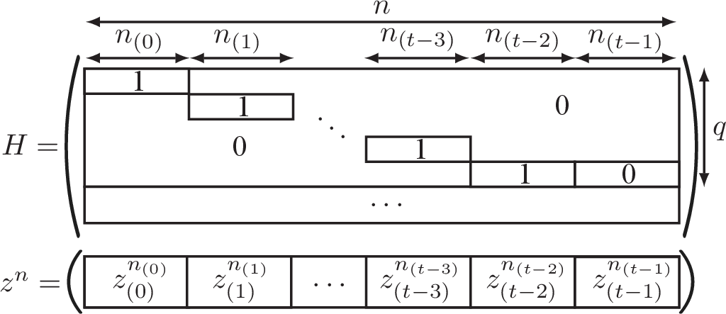
To restrict the noise effect generation by \(q\) constraints, the parity check matrix must contain \(q\) rows, of which at most one row has a \(1\) at each bit position. We now discuss such a requirement in more detail. In each of the first \(q\) rows of \(H\), the columns that contain a \(1\) in a specific row and the columns that contain a \(0\) in all \(q\) rows are partitioned into \(t = q+ 1\) segments, which are index sets \[\begin{align} \mathcal{S}_{(j)}&= \{i: i \in [n], H_{j+1, i} = 1\}, \; \text{for \(j \in \{0, \dots, t-2\}\),}\\ \mathcal{S}_{(t-1)} &= \{i: i \in [n], H_{j^\prime, i} = 0 \; \forall j^\prime \in [q]\}. \end{align}\] To simplify notation later for the proposed generalization, the indexing of segments begins at \(0\). Segmented GRAND requires that the parity check matrix can be transformed such that \(\mathcal{S}_{{(j)}} \cap \mathcal{S}_{{(j^\prime)}} = \emptyset\) for all \(j\neq j^\prime\), as visualized in Figure 1 after column permutation. Throughout the paper, we permute the columns of the parity check matrix such that segment bits are grouped for visualization.
We denote segment-specific properties via a subscript in brackets, e.g., \({(j)}\): \(n_{(j)}\mathrel{\vcenter{:}}= |\mathcal{S}_{(j)}|\) denotes the length of the \(j\)-th segment. \(e_{(j)}^{n_{(j)}} = (e_i)_{i \in \mathcal{S}_{(j)}}\) and \(z_{(j)}^{n_{(j)}} = (z_i)_{ i \in \mathcal{S}_{(j)}}\) are subsequences of the true noise effect \(e^n\) and current noise effect query \(z^n\), respectively, containing the bit values at the positions of segment \(j\), ordered by their original index \(j\). We refer to these subsequences of noise effects as subeffects. Let \(z_{{(j)},i}\) denote the \(j\)-th entry of \(z^{n_{(j)}}_{(j)}\). The quantities \[w_{\text{H}, {(j)}} = \sum_{i = 1}^{n_{(j)}} z_{{(j)},i}, \quad w_{\text{L},{(j)}} = \sum_{i=1}^{n_{(j)}} i z_{{(j)},i}, \quad p_{(j)}= \Phi(z^{n_{(j)}}_{(j)}),\] denote the HW, LW, and parity of the \(j\)-th subeffect \(z^{n_{(j)}}_{(j)}\) of the current guess \(z^n\) and \(w_{\text{H}}^t, w_\text{L}^t\) and \(p^t = (p_{(j)})_{j=0}^{t-1}\) denote the corresponding vectors. We refer to the sum of the subeffects logistic weights as total LW \(w_\text{T} = \sum_{j=0}^{t-1} w_{\text{L},{(j)}}\). Since the segments are a partition of \([n]\), the subeffects form a segmentation of \(z^n\) and \(e^n\), respectively. For instance, for \(z^n\): \(z^n = (z^{n_{(0)}}_{(0)} | z^{n_{(1)}}_{(1)} | \dots | z^{n_{(t-1)}}_{(t-1)}).\)
Rowshan and Yuan observed that for this particular structure, the first \(q\) equations of 2 are fulfilled if and only if the parity of the \(j\)-th subeffect matches the \((j+1)\)-th syndrome, i.e., \(p_{(j)}= s_{j+1}\) for \(j \in \{0, \dots, q-1\}\). Segmented GRAND leverages this observation as follows: the outer iteration iterates over the total LW \(w_\text{T}\), similarly to ORBGRAND, followed by a two-level partitioning that generates the noise effects. In the outer partition, all integer partitions of a total LW \(w_\text{T}\) into \(t\) segments are generated: \(w_{\text{L}, {(0)}}, \dots, w_{\text{L}, {(t-1)}}\). For each segment \(j\), the inner partition generates all distinct integer partitions that sum up to \(w_{\text{L}, {(j)}}\), which correspond to the bit flip positions. By merging these segment-wise integer partitions, noise effects are constructed that, by design, fulfill the first \(q\) equations of 2 and have a total LW of \(w_\text{T}\).
3 Generalized Segmented GRAND↩︎
While Segmented GRAND demonstrates that segmentation can enable guesswork reduction, it can only constrain the guessing for parity check rows that are in a specific structure. In this section, we propose a generalized version of Segmented GRAND, termed GSegGRAND, that enables the extraction of multiple constraints for a wide range of linear codes. The basis of this algorithm is the balanced tree structure. We will first introduce the tree structure and the balanced tree structure in Sec. 3.1, followed by the corresponding decoding algorithm in Sec 3.2. In addition, a systematic procedure to transform most practical codes into a balanced tree structure will be provided in Sec. 3.3. Finally, additional implementation details of the decoding algorithm are provided in Sec. 3.4.
3.1 Balanced Tree Structure↩︎
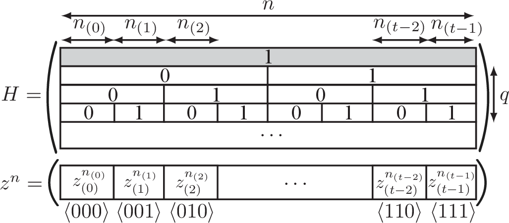
For a binary string \(v^q= (v_1,\dots,v_q) \in \mathbb{F}_2^q\), we define its integer value as \(\langle v_1 v_2 \dots v_q \rangle \mathrel{\vcenter{:}}= \sum_{i=1}^qv_i 2^{q-i}.\) We say that the first \(q\) rows of a parity-check matrix \(H\) are in tree structure if the columns of \(H\) are arranged in ascending order of their first \(q\) entries [33] (see Fig. 2), i.e., \[i < i^\prime \Rightarrow \langle H_{1, i} H_{2, i} \dots H_{q,i} \rangle \leq \langle H_{1, i^\prime} H_{2, i^\prime} \dots H_{q,i^\prime} \rangle.\] Any given \(H\) can be transformed into a tree structure by permuting its columns so that columns with identical first \(q\) entries are grouped into a segment \(j\), where \(j\) is the integer represented by those \(q\) binary entries. More explicitly, two columns \(i,i^\prime\) are put in the same segment \(j\) if \(j= \langle H_{1,i} H_{2,i} \dots H_{q,i} \rangle = \langle H_{1,i^\prime} H_{2,i^\prime} \dots H_{q,i^\prime} \rangle\). This yields at most \(t = 2^q\) segments. To leverage this structure, we index segment \(j = \langle v_1 \dots v_q \rangle \in \{0, \dots, t-1\}\) interchangeably by its decimal \(j\) or binary representation \((v_1,\dots,v_q)\). Hence, for a segment parity we may write either \(p_{(j)}\) or \(p_{(\langle v_1 v_2 \dots v_q \rangle)}\). Analogous to Segmented GRAND, the index set of segment \(\langle v_1 \dots v_q \rangle\) is given by \[\mathcal{S}_{(\langle v_1 \dots v_q \rangle)} = \{i \in [n]: H_{1:q, i} = (v_1, \dots, v_q)\}.\] As defined in Sec. 2.0.7, \(n_{(j)}, z_{(j)}^{n_{(j)}}, w_{\text{L},{(j)}}, w_{\text{H},{(j)}}\) and \(p_{(j)}\) denote length, subeffect, LW, HW and parity of segment \(j\). The tree structure is balanced if all \(t = 2^q\) segments exist and the segments’ lengths are approximately equal: \(n_{(\langle v_1 \dots v_q \rangle)} \approx n / t\). In the following, we assume that the code’s parity check matrix is in balanced tree structure. While this may appear restrictive, Sec. 3.3 demonstrates that a wide range of linear codes can be rewritten into this form.
By segmenting \(z^n\) into subeffects, the first \(q\) rows of \(s^{n-k} = H z^n\) in 2 can be written as a system of binary linear equations of the segment parities \(p^t\): \[\label{eqn:system} \begin{align} s_u &= \bigoplus_{i=1}^n H_{u, i} z_i = \bigoplus_{(v_1, \dots, v_q) \in \mathbb{F}_2^q} \bigoplus_{i=1}^{n_{(\langle v_1 \dots v_q \rangle)}} v_u z_{{(\langle v_1 \dots v_q \rangle)}, i} \\ &= \bigoplus_{\substack{ (v_1,...,v_{q}) \in \mathbb{F}_2^{q}: \\ v_u = 1 }} p_{(\langle v_1 \dots v_q \rangle)}, \end{align}\tag{8}\] for each \(u \in [q]\). In the second equality, we group terms segment-wise and use the fact that \(H_{u, i} = v_u\) for all bit positions \(i\) belonging to segment \(\langle v_1 \dots v_u \dots v_q \rangle\).
For even-weight codes, we extend the tree structure by an additional all-one row (see gray row in Fig. 2). To maintain a unified notation for both standard and extended tree structure, we denote the syndrome associated with this row by \(s_0:=\bigoplus_{i=1}^n y_{\text{hd},i}\). Without increasing the number of required segments, the all-one row introduces an additional constraint for the noise effect generation: \[\label{eqn:system3} s_0 = \bigoplus_{(v_1,...,v_{q}) \in \mathbb{F}_2^{q}} p_{(\langle v_1 \dots v_q \rangle)}\tag{9}\] which ensures that each generated noise effect will lead to a candidate codeword with even HW.
We call a vector of segment parities \(p^t=(p_{(0)}, \dots, p_{(t-1)})\) that fulfill 8 (and 9 in the case of the extended structure) a valid parity configuration for a given syndrome \(s^{n-k}\) and parity check matrix \(H\). Accordingly, a vector of HWs \(w_{\text{H}}^t = (w_{\text{H},{(0)}}, \dots, w_{\text{H}, {(t-1)}})\) whose parities form a valid parity configuration is called a valid HW configuration. By construction, any noise effect \(z^n\) whose subeffects HWs form a valid HW configuration automatically fulfills \(H_{1:q, :} z^n = (s_1,\ldots,s_q) = s_1^q\) (or \(H_{0:q, :} z^n = (s_0,s_1,\ldots,s_q) = s_0^q\) for the extended structure).

To efficiently iterate through valid parity configurations, we observe that the parities of the segments whose binary representation contains a single \(1\), i.e., the unit vectors, appear in exactly one equation of 8 . Thus, we can explicitly solve for these parities by isolating them on the left-hand side as shown in 3 in Alg. [alg:comp-unit-parity]. We refer to the parities on the left-hand side as unit parities \(p_{\text{u}}^q= \big(p_{(\langle v_1, \dots, v_q \rangle)} : \sum_{i=1}^n v_i = 1\big),\) and those on the right-hand side as non-unit parities \(p_{\text{nu}}^{t-q-1} = \big(p_{(\langle v_1, \dots, v_q \rangle)} : \sum_{i=1}^n v_i > 1\big).\) Note that \(p_{(0)}\) is not part of 3 and neither a unit nor non-unit parity. Together, \(p_{\text{u}}^q\), \(p_{\text{nu}}^{t-q-1}\), and \(p_{(0)}\) partition the parity configuration \(p^t = \texttt{Concatenate}(p_{(0)}, p_{\text{nu}}^{t-q-1}, p_{\text{u}}^q),\) where \(\texttt{Concatenate}\) combines the subvectors into the full parity configuration.
Given a set of known non-unit parities \(p_{\text{nu}}^{t-q-1}\) and the received syndrome \(s^{n-k}\), Alg. [alg:comp-unit-parity] uniquely determines the unit parities \(p_{\text{u}}^q\) that in combination with \(p_{\text{nu}}^{t-q-1}\) form a valid parity configuration. To iterate over all valid parity configurations, we can therefore iterate over all combinations of the non-unit parities \(p_{\text{nu}}^{t-q-1}\) and compute the valid unit parities via Alg. [alg:comp-unit-parity], which can be efficiently implemented as a binary matrix multiplication over \(\mathbb{F}_2\).
Once \(p_{\text{nu}}^{t-q-1}\) is known it remains to determine \(p_{(0)}\). Let \(\mathcal{P}_{(0)} \subset \mathbb{F}_2\) denote the feasible values of \(p_{(0)}\) that, together with \(p_{\text{u}}^q\) and \(p_{\text{nu}}^{t-q-1}\), form a valid parity configuration. The computation of \(\mathcal{P}_{(0)}\) is given in Alg. [alg:comp-zero-parity]:

the standard tree structure does not enforce any constraint on \(p_{(0)}\), and we therefore additionally iterate over both values: \(\mathcal{P}_{(0)} = \{0, 1\}\). In extended tree structure, \(p_{(0)}\) is constrained by 9 which can be solved for \(p_{(0)}\) with \(p_{\text{u}}^q, p_{\text{nu}}^{t-q-1}\) and \(s_0\) on the right hand side.
3.2 Decoding Algorithm↩︎
To leverage the segment parity constraints in 8 and 9 , we follow Segmented GRAND [27] and, at each time, generate one subeffect for each segment, followed by combining the subeffects into one complete noise effect. Let \(|\tilde{L}_{{(j)},i}|\) denote the random variable of the reliability of the \(i\)-th bit in segment \(j\) and let \(|\tilde{\ell}_{{(j)}, i}|\) be its realization. As pointed out by [34]6, the q-th sample quantile of the reliabilities in every segment \(j\), \(|\tilde{L}_{{(j)},1}|, |\tilde{L}_{{(j)},2}|, \dots, |\tilde{L}_{{(j)},n_{(j)}}|\), converges to \(F^{-1}(q)\) as \(n_{(j)}\rightarrow\infty\), where \(F\) is the cumulative distribution function (CDF) of \(|\tilde{L}_{{(j)},i}|\) and \(F^{-1}(s) = \inf\{u: F(u) \geq s\}\). As a result, we expect that the plot of rank-ordered reliabilities \(|L_{{(j)}, i}|\) versus the rank \(i\) is approximately the function \[\label{eqn:approx} |L_{{(j)}, i}| \approx F^{-1}(i/n_{(j)}), \qquad \text{for \(i \in [n_{(j)}]\)},\tag{10}\] where we denote rank-ordered reliabilities without tilde. Duffy et al. [4] observed that for practical noise effect generation, the rank-ordered reliabilities can be approximated by a line with intercept \(0\). Applying a first-order Taylor approximation to 10 with intercept \(0\) results in a linear relation between rank and reliabilities \[\begin{align} |L_{{(j)},i}| &\approx F^{-1}(i/n_{(j)}) \approx \beta_{(j)}i, \\ \quad \beta_{(j)}&= \frac{1}{n_{(j)}} \frac{d F^{-1}(s)}{d s} = \frac{(F^{-1})^\prime}{n_{(j)}} \end{align}\] for \(i \in [n_{(j)}]\) and \(j \in \{0, \dots, t-1\}\), where \(\beta_{(j)}\) denotes the slope of the \(j\)-th segment. Since the tree structure is balanced (i.e., \(n_{(j)}\approx n / t\)) and \(F\) is segment independent, the slopes \(\beta_{(j)}\) are all approximatly equal: \(\beta_{(0)} \approx \dots \approx \beta_{(t-1)}\). With this approximation, the reliability of a noise effect \(z^n\) in 1 for a realization \(\ell_{{(j)},i}\) becomes \[\label{eqn:rel-gen-seg-grand} \begin{align} \text{Rel}(z^n) &= \sum_{j=0}^{t-1} \sum_{i=1}^{n_{(j)}} |\ell_{{(j)}, i}| z_{{(j)}, i} \approx \beta_{(0)} w_\text{T}. \end{align}\tag{11}\] Owing to the balanced property of the tree structure, we can factor the common slope \(\beta_{(0)}\), which makes the reliability of \(z^n\) proportional to its total LW \(w_\text{T}\). Combined with 1 and 11 , this shows that the probability of a noise effect decreases monotonically with increasing total LW \(w_\text{T}\). Consequently, constrained noise effects with equal probability can be generated by merging independently generated subeffects that share a valid HW configuration and whose segment-wise LWs sum to the same total \(w_\text{T}\).
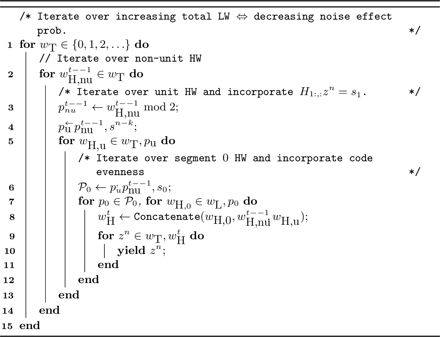
Algorithm 5 describes the high-level components of the GSegGRAND algorithm: an outer iteration iterates over increasing total LW \(w_\text{T}\) to create noise effects in decreasing order of probability. For each \(w_\text{T}\), the algorithm
generates valid HW configurations \(w_{\text{H}}^t\) corresponding to the received syndrome \(s^{n-k}\). Specifically,
the HW generator \(\texttt{HWGen}(w_\text{T})\) iterates over all possible HW
assignments \(w_{\text{H,nu}}^{t-q-1}\) for the non-unit segments, for which the current total LW \(w_\text{T}\) can
be achieved (see the implementation details in Sec. 3.4 for details). For each \(w_{\text{H,nu}}^{t-q-1}\), UnitParityComp and ZeroParityComp given in
Alg. [alg:comp-unit-parity] and Alg. [alg:comp-zero-parity], respectively, determine the parities of the unit segments and of segment \(0\) that result in a valid HW configuration. For these segments, \(\texttt{HWGen}(w_\text{T}, p_\text{u}^q)\) and \(\texttt{HWGen}(w_\text{T}, p_{(0)})\) only iterate over the
HWs with correct parity \(p_\text{u}^q\) and \(p_{(0)}\), skipping every second HW for each segment. For each valid HW configuration \(w_{\text{H}}^t\), the 2D Landslide algorithm \(\texttt{2DSegLS}(w_\text{T}, w_\text{H}^t)\) (see Sec. 3.4) generates all noise effects of this HW configuration
\(w_{\text{H}}^t\) and LW \(w_\text{T}\) by partitioning the LW among the segments.
3.2.1 Example: Even-weight Code with 3 Constraints↩︎
Figure 6 visualizes this process for an even-weight code and \(3\) constraints. In this case, there exist only one non-unit segment \(j=\langle 11
\rangle\) whose HW can be assigned freely. For each \(w_{\text{H}, {(\langle 11 \rangle)}}\), the parities of the unit segments follow directly as: \[\begin{align} p_{{(\langle 10
\rangle)}} = s_2 \oplus p_{(\langle 11 \rangle)}, \quad p_{{(\langle 01 \rangle)}} = s_1 \oplus p_{(\langle 11 \rangle)}
\end{align}\] where \(p_{(\langle 11 \rangle)} = w_{\text{H},{(\langle 11 \rangle)}} \bmod 2\), allowing the HW generator to skip every second
HW with incorrect parity. Likewise, the HW generator for the \(0\) segment
restricts generation of subeffects to parities of \[\begin{align} p_{(\langle 00 \rangle)} &= s_0 \oplus p_{(\langle 10 \rangle)} \oplus p_{(\langle 01 \rangle)} \oplus p_{(\langle 11 \rangle)}.
\end{align}\] For a given set of HWs, 2DSegLS produces subeffects with corresponding HW whose
LWs sum to \(w_\text{T}\), which are merged and sent to the codebook checker.

3.3 Balanced Tree Transformation↩︎
As outlined in Sec. 3.2, the decoder operates on an approximately balanced tree structure, i.e., the segments have approximately equal length. In this section, we propose a transformation which we call balance tree transformation that approximately balances parity check matrices. The idea of this transformation is to apply a random invertible matrix to the parity check matrix \(H \in \mathbb{F}_2^{m \times n}\), where \(m \mathrel{\vcenter{:}}= n - k\), before rewriting it in tree structure. The probability that we get a transformed matrix with the desired property is bounded below by \(0.22\) as \(m\rightarrow \infty\). To provide a theoretical validation, Theorem 1 is first proved without invertible assumption on the random transformation. After Theorem 1, we will restrict to invertible random transformation so that the rewritten code is equivalent to the given code.
Theorem 1. Let \(H^{m,\kappa m}\) be a given \(m\times \kappa m\) binary matrix, for \(\kappa\in \mathbb{N}\). Separate \(H^{m,\kappa m}\) into \(\kappa\) non-overlapping sub-matrices with dimension \(m \times m\) and denote each of the sub-matrices as \(H^{m,\kappa m}_{\{j\}}\). Let \[\mathcal{H}^{m,\kappa m}:= \{H^{m,\kappa m}|H^{m,\kappa m}_{\{j\}} \text{ is invertible for all }j\leq \kappa \}\] be the set of parity check matrices whose sub-matrices are all invertible. Let \(\widetilde{H}^{m,\kappa m}=A^{m,m}H^{m,\kappa m}\), where \(A^{m,m}\in\mathbb{F}_2^{m\times m}\) is a random binary matrix whose entries are i.i.d Bernoulli distributed with rate \(0.5\). Then,
Each \(\widetilde{H}^{m,\kappa m}_{\{j\}}=A^{m,m}H^{m,\kappa m}_{\{j\}}\) is uniformly distributed over all binary \(m\times m\) matrices given \(H^{m,\kappa m}\in\mathcal{H}^{m,\kappa m}\) and hence can be treated as matrix with i.i.d entries from Bernoulli distribution with rate \(0.5\).
The rows in \(\widetilde{H}^{m,\kappa m}\) are independent to each other.
Given \(\delta>0\), let \(\{H^{m,\kappa m}\}_{m\in\mathbb{N}}\) be any given sequence of parity check matrices such that \(H^{m,\kappa m}\in\mathcal{H}^{m,\kappa m}\) for all \(m\), and let \(H^{m,\kappa m}_{{\{j\}},i,s}\) denote the entry of \(H^{m,\kappa m}_{\{j\}}\) at the \(i\)-th row and \(s\)-th column, then \[\begin{align} \lim_{m\rightarrow \infty}P\left(\bigcup_{j=1}^{\kappa}\bigcup_{i=1}^m\Bigg\{\left|\sum_{s=1:m}\frac{\widetilde{H}^{m,\kappa m}_{\{j\},i,s}}{m}-0.5\right|>\delta\Bigg\}\right)=0. \end{align}\]
Proof. 1) Let \(\widetilde{h}\in\mathbb{F}_2^{m\times m}\) be any matrix. Then, \[\begin{align} &P\left(\widetilde{H}^{m,\kappa m}_{\{j\}} = \widetilde{h}|H^{m,\kappa m}_{\{j\}}\right) \stackrel{(\text{a})}{=} P\left(A^{m, m}H^{m,\kappa m}_{\{j\}}=\widetilde{h}|H^{m,\kappa m}_{\{j\}}\right)\\ &\stackrel{(\text{b})}{=} P\left(A^{m,m}=\widetilde{h}[H^{m,\kappa m}_{\{j\}}]^{-1} \middle|H^{m,\kappa m}_{\{j\}}\right)=2^{-m^2}. \end{align}\] (a) uses the invertibility of the sub-matrix \(H^{m,\kappa m}_{\{j\}}\) as \(H^{m,\kappa m}\in\mathcal{H}^{m,\kappa m}\). (b) holds since the \(m^2\) entries of \(A^{m,m}\) are i.i.d. Bernoulli distributed with rate \(0.5\) so it equals \(\widetilde{h}[H^{m,\kappa m}_{\{j\}}]^{-1}\) with probability \((1/2)^{m^2}\). Hence \(\widetilde{H}^{m,\kappa m}_{\{j\}}=A^{m, m}H^{m,\kappa m}_{\{j\}}\) is uniformly distributed over all binary \(m\times m\) binary matrices. With coupling technique [35], \(\widetilde{H}^{m,\kappa m}_{\{j\}}\) can be treated as a matrix with i.i.d entries from Bernoulli distribution with rate \(0.5\). This completes the first claim.
2) Notice that \(\widetilde{H}^{m,\kappa m}_{i,j}=\sum_{s=1}^m A^{m,\kappa m}_{i,s}H^{m,\kappa m}_{s,j} \mod 2\). Since \(H^{m,\kappa m}\) is given and the rows of \(A^{m,\kappa m}\) are independent, the rows of \(\widetilde{H}^{m,\kappa m}\) are also independent. This completes the second claim.
3) To prove the third claim, we consider the sum \(S_{\{j\}, i, m} = \sum_{s=1}^m \widetilde{H}^{m,\kappa m}_{\{j\},i,s} / m\) whose summands are bounded between \(0\) and \(1/m\), and according to claim 1, i.i.d. Bernoulli-distributed with rate \(0.5\). Hence, the expected value of \(S_{\{j\}, i, m}\) is \(0.5\) and applying Hoeffding’s inequality [36] to \(S_{\{j\}, i, m}\) yields, given \(\delta > 0\), \(P(|S_{\{j\}, i, m} - 0.5| > \delta) \leq 2 \exp(-2\delta^2 m).\) Applying the union bound to \(\bigcup_{i=1}^m\{|S_{\{j\}, i, m} - 0.5| > \delta\}\) results in \[\begin{align} \lim_{m\rightarrow \infty}P\left(\bigcup_{i=1}^m \Bigg\{ \left|\sum_{s=1}^m\frac{\widetilde{H}^{m,\kappa m}_{\{j\},i,s}}{m}-0.5\right| > \delta \Bigg\} \right)=0, \end{align}\] because \(\lim_{m \to \infty} \sum_{i=1}^m 2\exp(-2\delta^2m) = 0\). This means we can expect that a sub-matrix has almost half the number of ones and zeros within each row. By the union bound, we are able to conclude that this happens to all sub-matrices of \(\widetilde{H}^{m,\kappa m}\) simultaneously as we have a fixed code rate \(1/\kappa\), which finishes the third claim. ◻
The first result of Theorem 1 states that a parity check matrix, whose sub-matrices are invertible, can be transformed into a random matrix whose entries in each sub-matrix can be treated as i.i.d. variables with equal probability of being one or zero. This further leads to the properties stated in the second and third results. Choosing \(\delta\) close to zero and applying the third result shows that as \(m\rightarrow\infty\), we can expect that the number of ones is approximately the same as the number of zeros in each row of \(\widetilde{H}^{m,\kappa m}\), while the coderate is constant: \(r = 1 - 1 / \kappa\). Together with the fact that each row is independent in \(\widetilde{H}^{m,\kappa m}\), we can expect that each segment length \(n_{(\langle v_1 \dots v_q \rangle)}\) of \(\widetilde{H}^{m,\kappa m}\) in tree structure is approximately the same, that is, the set of columns are divided into subsets with approximately equal sizes. The name balanced tree transformation is given based on this property.
To retain the same structure of the code represented by \(H^{m,\kappa m}\), we further require that the random transformation \(A^{m,m}\) is invertible. The probability that a random binary matrix \(A^{m, m}\) is invertible is bounded below by 0.22 as \(m\rightarrow \infty\) [37]–[39]. Therefore, by the union bound, the probability that \(A^{m,m}\) is invertible and each segment length \(n_{(j)}\) of \(\widetilde{H}^{m,\kappa m}\) in tree structure is approximately the same is bounded below as \(m\rightarrow \infty\). This establishes that, in the limit, we can transform parity check matrices into tree structure with desired properties with positive probability bounded below. We call the procedure of multiplying \(H\) by a random matrix the balance transformation. Additionally, the procedure of balance transformation followed by rewriting the resulting matrix into tree structure is called balanced tree transformation.
As the balanced tree transformation is invertible and hence does not change the code, we only need to apply the transformation once for any given parity check matrix and use the rewritten parity check matrix and generator matrix for application. Therefore, this transformation will not add additional complexity to the decoding.
3.4 Implementation Details↩︎
An important implementation detail is that the HW configurations are restricted to those configurations for which the given total LW \(w_\text{T}\) is realizable; otherwise, the algorithm would generate configurations for which 2D Landslide cannot find valid noise effects. This is particularly important as GSegGRAND supports multiple parity check constraints requiring numerous segments, which can lead to a large number of invalid HW configurations if not handled properly. To obtain bounds efficiently, GSegGRAND places the parity-check constraints in its outer loops and performs logistic-weight partitioning within its inner loops. This is in contrast to Segmented GRAND, which first partitions the LW before enforcing parity constraints. Furthermore, the iteration over error pattern bases (segments without bit flips) used in [27] is implicitly incorporated in the proposed approach: a segment with HW \(0\) naturally corresponds to an empty segment, eliminating the need for an explicit base iteration.
This iteration order provides an additional advantage: because the structure of the proposed algorithm on the segment level corresponds to ORBGRAND, i.e., first HW iteration followed by LW partitioning, the decoder can build directly upon the existing Landslide algorithm, for which efficient hardware implementation already exists [9]. The following section outlines how the outer HW generator and inner 2D Landslide algorithm are realized.
3.4.1 Hamming Weight Generator (HWGen)↩︎
The HW generation in Alg. 5 is executed through multiple stages to incorporate the parity check constraints. Note that for the \(j\)-th segment, a subeffect with HW \(w_{\text{H},{(j)}}\) can only have LWs \(w_{\text{L},{(j)}}\) within the range, \(w_{\text{L,min},{(j)}} \leq w_{\text{L},{(j)}} \leq w_{\text{L,max},{(j)}}\), where [4] \[\begin{align} w_{\text{L,min}, {(j)}} &= \frac{w_{\text{H},{(j)}} (w_{\text{H},{(j)}} + 1)}{2}, \\ w_{\text{L,max}, {(j)}} &= \frac{n_{(j)}(n_{(j)}+ 1)}{2} \\ &\phantom{=} - \frac{(n_{(j)}- w_{\text{H},{(j)}}) (n_{(j)}- w_{\text{H},{(j)}} + 1)}{2}. \end{align}\] A given HW configuration \(w_\text{H}^t\) therefore has noise effects with LW within the sum of the segment-wise bounds \[\label{eqn:bounds-log-weight} \sum_{j=0}^{t-1} w_{\text{L,min},{(j)}} \leq w_\text{T} \leq \sum_{j=0}^{t-1} w_{\text{L,max},{(j)}}.\tag{12}\] 2D Landslide can find valid noise effects if the current total LW \(w_\text{T}\) is within these bounds. We ignore the upper bound, as GSegGRAND most of the time terminates for a relatively small \(w_\text{T}\) and the bound does not restrict \(w_\text{H}^t\) in practice. To incorporate the lower bound, assume that the HW generator has already chosen the HW for a subset of segments \(j_1, \dots, j_r\). The lower bound of 12 enforces an upper bound on the HW of the next segment \(j_{r+1}\) \[\label{eqn:cond} \frac{ w_{\text{H},{(j_{r+1})}} (w_{\text{H},{(j_{r+1})}}+1) }{2} = w_{\text{L,min},{(j_{r+1})}} \leq w_\text{T} - \sum_{i=1}^{r} w_{\text{L,min},{(j_i)}}.\tag{13}\]
In practice, the HW generator increases a HW \(w_{\text{H},{(j_{r+1})}}\) starting from \(0\) as long as 13 is fulfilled. As soon as 13 is violated, \(w_{\text{H},{(j_{r+1})}}\) is set to \(0\) and the generator increases the previous HW \(w_{\text{H},{(j_{r})}}\) by one. If the increase also violates 13 it moves up another level. If the HW \(w_{\text{H}, {(j_r)}}\) corresponds to a unit segment, the generator uses the same stopping condition but starts at the precalculated parity \(p_{(j_r)}\) instead of \(0\) and increases the HW by \(2\) each step. This ensures that the generator implicitly only generates HWs of correct parity.
3.4.2 2D Landslide (2DSegLS)↩︎
The 2D Landslide algorithm \(\texttt{2DSegLS}(w_\text{T}, w_{\text{H}}^t)\) partitions the total LW \(w_\text{T}\) among the segments: \(w_\text{L}^t = (w_{\text{L}, {(0)}}, \dots, w_{\text{L}, {(t-1)}})\) and generates noise effects whose subeffects have HW \(w_{\text{H}, {(j)}}\) and LW \(w_{\text{L}, {(j)}}\). To realize this, the algorithm runs, for each integer partition \(w_\text{L}^t\), the Landslide algorithm (see Sec. 2.0.4) on each segment. In practice, this forms a nested enumeration over all combinations of subeffects: each landslide generator \(\text{LS}(w_{\text{H}, {(j)}}, w_{\text{L}, {(j)}})\) produces its first noise effect and the last generator iterates through all its effects. When it runs out of effects, it resets, and the preceding landslide generator advances to its next noise effect. This process continues in a nested manner until the first generator has no remaining effects. After each enumeration, the subeffects are merged and tested by the codebook checker.
4 Soft-output Calculation for Constrained Guessing↩︎
In this section, we outline how SOGRAND’s SO computation can incorporate constrained guessing, enabling us later to use GSegGRAND as a component decoder for turbo product decoding with minimal performance loss (less than 0.2 dB) over ORBGRAND without constrained guessing. We explain first the core idea for noise effect skipping in SOGRAND, which was proposed in [30], and then apply the idea to GSegGRAND.
Constrained guessing restricts the noise effect generation to noise effects \(z^n\) to a subspace \(\Gamma\subset \mathbb{F}_2^n\). If a linear code is even, i.e., has only codewords of even weight, ORBGRAND can restrict generation to noise effects of correct parity \(s_0 = \Phi(y_{\text{hd}}^n) = \Phi(e^n)\): \(\Gamma_{\text{ORB},s_0} = \{z^n : \Phi(z^n) = s_0\},\) by leveraging Landslides’ ability to generate effects of specific HW. Feng et al. noticed that in this case, the quality of SOGRAND’s SO can be improved by conditioning the noise effect probability terms in 5 on the parity constraint \(\Gamma_{\text{ORB},s_0}\) [30]. That means for a general constraint space \(\Gamma\), we have \[\label{eqn:cond-noise-prob} P_{E^n | Y^n, E^n \in \Gamma}\Big(z^n | y^n\Big) = \mathbb{1}_{\{z^n \in \Gamma\}} P_{E^n | Y^n}(z^n | y^n) / \psi,\tag{14}\] where \(\psi \mathrel{\vcenter{:}}= P_{E^n | Y^n}(\Gamma| y^n) = \sum_{z^n \in \Gamma} P_{E^n | Y^n}(z^n | y^n)\) and \(\mathbb{1}_{\{z^n \in \Gamma\}}\) denotes the indicator function, which is \(1\) if \(z^n \in \Gamma\) and \(0\) otherwise. Replacing the unconditional probabilities \(P_{E^n | Y^n}(z^n | y^n)\) in 5 with 14 and expanding the fractions by \(\psi\) results in the improved SO expressions \[\label{eqn:block-so-updated} \begin{align} \hat{P}_{C^n | Y^n}(\hat{c}^n | y^n) &= \frac{ P_{E^n | Y^n}\left(\hat{c}^n \oplus y_\text{hd}^n | y^n\right) }{ P_\mathcal{L}+ (\psi - P_{\text{noise}}) 2^{-(n-k - \lambda)} }, \\ \hat{P}_{C^n | Y^n}(\mathcal{C} \setminus \mathcal{L} | y^n) &= \frac{ (\psi - P_{\text{noise}}) 2^{-(n-k - \lambda)} }{ P_\mathcal{L}+ (\psi - P_{\text{noise}}) 2^{-(n-k - \lambda)} }, \end{align}\tag{15}\] where \(\hat{c}^n \in \mathcal{L}\) and \(\lambda=1\) while \(P_{\text{noise}}\) and \(P_\mathcal{L}\) are given by 4 .
In addition to \(\psi\), 15 introduces the additional parameter \(\lambda \in \mathbb{N}\). If only the even code property is leveraged, \(\lambda=1\) as mentioned. If more constraints are leveraged as with Segmented GRAND or GSegGRAND, \(\lambda\) should increase accordingly. To understand its purpose, we recall how SOGRAND SO calculation works: the optimal SO calculation normalizes each codeword’s a posteriori probability by the codebooks probability mass \(\sum_{\hat{c}^n \in \mathcal{C}} P_{E^n | Y^n}\left(\hat{c}^n \oplus y_\text{hd}^n | y^n\right)\). Since list decoding only reveals the probability mass \(P_\mathcal{L}\) of the codewords in the list, SOGRAND assumes that the remaining \(2^k - |\mathcal{L}|\) codewords are uniformly distributed among the \(2^n - g\) unexplored noise effects, where \(g\) denotes the number of explored noise effects. This corresponds to an approximate probability mass of \(2^{-(n-k)}\) times the unexplored noise effect probability \(1 - P_{\text{noise}}\). In contrast, a GRAND variant that incorporates \(\lambda\) parity check constraints only guesses within a set of \(2^{n - \lambda}\) noise effects while the number of unexplored codewords stays constant, resulting in the factor \(2^{-(n-k-\lambda)}\).
When the even code structure is leveraged as in [30], \(\lambda=1\) and \(\psi\) is equal to the a posteriori probability of the noise effect parity, which can be directly calculated via [40] \[\begin{align} \psi &= P_{E^n | Y^n}(\Gamma_{\text{ORB},s_0} | y^n) = P_{\Phi(E^n) | Y^n}(s_0| y^n) \\ &= \frac{1}{2} \Big(1 + (-1)^{s_0} \prod_{i=1}^n (1-2 P_{E_i | Y_i}(1 | y_i))\Big), \end{align}\] where \(S_0 = \Phi(E^n)\) is the random variable of the global parity. While [30] showed that this modification improves the SO quality, it is unclear whether the better SO quality affects TPC decoding. In this paper, we apply the modification to TPC and demonstrate that the modification is essential for GRAND component decoding with constrained guessing as the the original SO calculation can lead to high error floors for certain codes or performance loses of up to 0.5 dB.
To apply this concept to Segmented GRAND and GSegGRAND, we need to find an efficient way to calculate the probability mass \(\psi = P_{E^n | Y^n}(\Gamma| y^n)\) of all noise effects \(\Gamma\) over which the algorithms carry out guesswork. Segmented GRAND and GSegGRAND with standard tree structure restrict their guessing space by \(q\) linearly independent constraints, and the extended tree structure restricts the space by \(q+1\) constraints. Hence, we set \(\lambda = q\) or \(\lambda = q+ 1\) accordingly.
The constraint space of Segmented GRAND is given by \[\Gamma_{\text{Seg},s^{n-k}} = \{z^n : H_{1:q, :} z^n = s^{n-k}\} = \bigcap_{j=1}^q \Gamma_{\text{Seg},{(j)},s_j},\] where \(\Gamma_{\text{Seg},{(j)},s_j} = \{z^n: \Phi(z_{(j)}^{n_{(j)}}) = s_j\}\) is the constraint associated with segment \(j\). Since Segmented GRAND requires parity check equations with nonoverlapping \(1\)s for its constraint space, and the channel is memoryless, the individual constraints \(\Gamma_{\text{Seg},{(j)},s_j}\) are stochastically independent events \(\{E^n \in \Gamma_{\text{Seg},{(j)},s_j}\}\), resulting in a probability for \(\Gamma\) of \[\psi = P_{E^n | Y^n}(\Gamma_{\text{Seg},s^{n-k}} | y^n) = \prod_{j=1}^q P_{S_j | Y^n}\left(s_j| y^n\right),\] where \(S^{n-k} = H E^n\) is the syndrome random variable. The a posteriori probability of the segment’s parity can be directly calculated via [40] \[\begin{gather} \label{eqn:segmented-parity-prob} P_{S_j | Y^n}\left(s_j| y^n\right) = P_{\Phi\left(E^{n_{(j)}}_{(j)}\right) | Y^n}\left(s_j| y^n\right) \\ = \frac{1}{2} \Big(1 + (-1)^{s_j} \prod_{i=1}^{n_{(j)}} (1-2 P_{E_{{(j)},i} | Y_{{(j)},i}}(1 | y_{{(j)},i}))\Big), \end{gather}\tag{16}\] where \(e_{{(j)},i}\) and \(y_{{(j)},i}\) denote the \(i\)-th position of the \(j\)-th segment of the correct noise effect and received value.
GSegGRAND’s constraints space can be expressed by a linear system of parity check constraints (see Sec. 3.1): \(\Gamma_\text{GSeg} = \{z^n: \eqref{eqn:system}\}\) and \(\Gamma_\text{GSeg} = \{z^n: \eqref{eqn:system}, \eqref{eqn:system3}\}\) for the standard and extended tree structure, respectively, whose solutions are valid parity check configurations \(p^t\). Let \[\Gamma_{\text{GSeg},p^t} \mathrel{\vcenter{:}}= \left\{z^n: \forall j \in \{0, \dots, t-1\}, \Phi\left(z_{(j)}^{n_{(j)}}\right) = p_{(j)} \right\}\] denote the set of the noise effects whose subeffect parities form the parity configuration \(p^t\). Then, \(\Gamma_{\text{GSeg},p^t}\) form a partition of GSegGRAND constraint space \(\Gamma_\text{GSeg} = \bigcup_{p^t: \eqref{eqn:system}, [\eqref{eqn:system3}]} \Gamma_{\text{GSeg},p^t}\), where the union is over all valid parity check configurations \(p^t\) satisfying 8 and, for the extended tree structure, also 9 . By the same independence argument used for Segmented GRAND, the a posteriori probability of \(\Gamma_{\text{GSeg},p^t}\) factorizes as \[P_{E^n | Y^n}(\Gamma_{\text{GSeg},p^t} | y^n) = \prod_{j=0}^{t-1} P_{\Phi\left(E^{n_{(j)}}_{(j)}\right) | Y^n}\left(p_{(j)}| y^n\right),\] whose factors can each be calculated via 16 by replacing \(s_j\) with \(p_{(j)}\). Since the sets \(\Gamma_{\text{GSeg},p^t}\) form a partition of \(\Gamma_\text{GSeg}\), we obtain \[\label{eqn:sum-prob} P_{E^n | Y^n}(\Gamma_\text{GSeg} | y^n) = \sum_{p^t: \eqref{eqn:system}, [\eqref{eqn:system3}]} P_{E^n | Y^n}(\Gamma_{\text{GSeg},p^t} | y^n).\tag{17}\] where the sum is over \(p^t\) satisfying 8 and, for the extended tree structure, also 9 .
The valid parity check configurations in the sum of 17 can be efficiently iterated using UnitParityComp and ZeroParityComp given in Alg. [alg:comp-unit-parity] and Alg. [alg:comp-zero-parity], respectively, (see Sec. 3.1) and we can reuse the parity iterator framework on which GSegGRAND is built. Note that the partition by parity check configurations
enables the computation of \(P_{E^n | Y^n}(\Gamma_\text{GSeg} | y^n)\) by a small number of summations, avoiding the infeasible evaluation of all terms in \(\Gamma\). Specifically, for the
extended tree structure with \(q=1\) and \(q=2\) we can list and implement the summation explicitly as \(q=1\) has only one summand \(p^2 \in \{(s_0 \oplus s_1, s_1)\},\) and \(q=2\) has only two summands \[\begin{gather} p^4 \in \{ (s_0 \oplus s_1 \oplus s_2, s_2, s_1, 0), \\ (s_0 \oplus s_1 \oplus
s_2 \oplus 1, s_2 \oplus 1, s_1 \oplus 1, 1) \}.
\end{gather}\]
5 Results↩︎
ORBGRAND and GSegGRAND function with any channel that outputs LLR. To evaluate their performance in this section, we consider a binary-input additive Gaussian noise channel (BI-AWGN) that maps codewords \(c^n \in \mathcal{C}\) to the channel output \(y^n\) with \(y_i = (-1)^{c_i} + \xi_i\) for \(i \in [n]\). \(\xi_i\) are independent normal distributed noise samples with variance \(\sigma^2 = (2 E_\textrm{s} / N_0)^{-1}\), where \(E_\textrm{s} / N_0= r E_\textrm{b} / N_0\) and \(r\) is the code rate, resulting in the LLRs: \(\ell_i = 2 y_i / \sigma^2\).
5.1 Balancing↩︎
Theorem 1 analyzed balancing of parity check matrices for \(n \to \infty\). In this section, we demonstrate how balancing can be applied to concrete codes with finite \(n\), resulting in the balanced tree structures used for the numerical results. To balance a concrete parity check matrix \(H\), \(H\) is multiplied with invertible binary matrices \(A\) sampled uniformly at random, and the columns are permuted into tree structure. A transformation \(A H\) is accepted if the discrepancy \(\max_j |n_{(j)}- n / 2^t|\) between the segment lengths \(n_{(j)}\) and the optimal balancing is below a certain threshold. To obtain an extended balanced tree structure for even codes, we first add an additional all-one row as first row, apply Gaussian elimination and remove the resulting last all-zero row. Then, balancing is performed on all rows excluding the first one as described above. Note that the balancing only needs to be applied once offline and does not contribute to the decoding complexity. We observed that the decoding performance does not degrade for small discrepancies, especially when the code is long. For even-weight Hamming codes (e.g., the (32, 26) eBCH code in this work), by definition all rows of the parity check matrix can be represented in balanced tree structure and balancing is not required.
| Code | ||
| Discrepancy | ||
| Discrepancy | ||
| (256, 239) eBCH | 2 | 6.3 % |
| (128, 106) eBCH | 0 | 0 % |
| (32, 21) dRM | 0 | 0 % |
| (32, 26) eBCH | 0 | 0 % |
| (128, 110) CA-Polar code | 1 | 6.3 % |
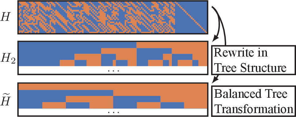
In this work, we demonstrate decoding with up to 8 segments and therefore balance up to \(4\) rows in extended tree structure. Table 2 lists the results of the balancing for \(4\) rows, and lists the absolute discrepancy \(\max_j |n_{(j)}- n / 2^t|\) and relative discrepancy \(\max_j |n_{(j)}- n / 2^t| / (n / 2^t)\): we achieve balancing with a maximal absolute discrepancy of \(2\) for (256, 239) eBCH code, \(1\) for the (128, 110) CRC-Assisted Polar (CA-Polar) code, and perfect balancing for all other codes. Figure 7 visualizes this process on the first \(4\) parity check rows of the (128, 106) eBCH code (matrix \(H\)), where orange and blue rectangles represents \(1\) and \(0\)s, respectively: the tree structure without rebalancing (\(H_2\)) has a strong imbalance. However, after balancing, the first \(4\) rows are perfectly balanced with \(8\) segments of lengths \(16\).
5.2 Decoding of Component Codes↩︎
We demonstrate the performance of GSegGRAND on the (128, 106), and (256, 239) eBCH codes, which are visualized in Fig. 8, and 9. In every legend entry, we denote the number of constraints that the decoder considers in brackets. Efficient decoding of the eBCH (256, 239) is particularly important as it serves as the component code of the OFEC code defined in the Open ROADM standard in optical communications [41]. [27] originally tested Segmented GRAND on the (128, 106) eBCH demonstrating that the required guesswork for it can be reduced by up to a factor of \(4\) by incorporating \(2\) constraints. Following up on this, we demonstrate GSegGRAND’s strength and incorporate up to \(4\) constraints.
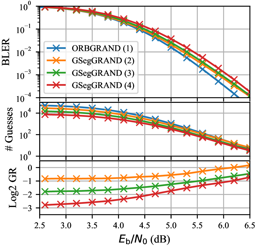
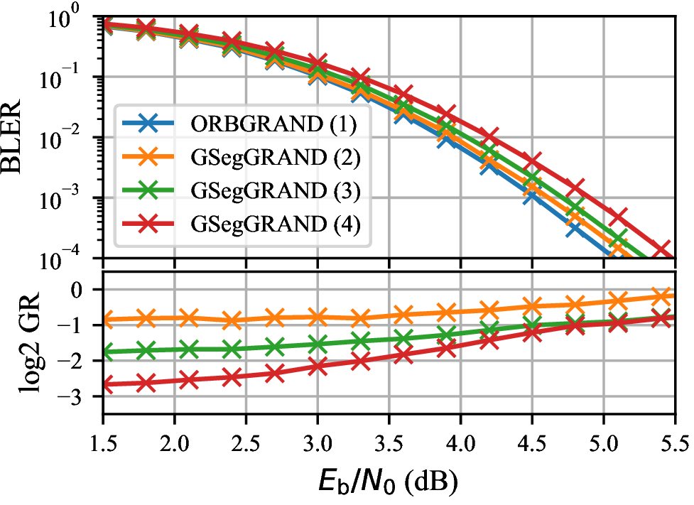
To compare all decoders at their maximal performance, we use an abandonment threshold of \(2^{n-k}\). This threshold is the average number of guesses until an incorrect codeword is found, and further guessing does in general not improve performance [2]. For GSegGRAND, we use 2, 4, and 8 segments, which take, for even-weight codes, \(2\), \(3\), and \(4\) constraints into account, respectively. Our baseline is ORBGRAND without segmentation, whose noise effect generator can incorporate \(1\) constraint if the code is even. We can therefore expect a maximal guesswork reduction of \(2^{-1}\), \(2^{-2}\), and \(2^{-3}\) compared to ORBGRAND. The upper plot of each figure shows the BLER vs \(E_\textrm{b} / N_0\) and the middle plot in Fig. 8 shows the average guesswork in \(\log_{10}\)-scale. We define the average guesswork as the average number of noise effect generations carried out during decoding until a codeword is found or decoding is abandoned. For clarity, we calculate the log2 GR, which is the ratio between the decoder’s and ORBGRAND’s average guesswork in \(\log_2\)-scale and plot them in the lower plot of each figure.
GSegGRAND experiences a slight performance loss at low SNR, which is caused by the independent generation of subeffects through which the relative ordering between bits of different segments is lost. More specifically, the lost is caused by the difference between 3 and 11 . However, this loss is exchanged for a guesswork reduction of up to \(2^3=8\) at low SNR, showing that GSegGRAND utilizes the constraints fully. This low SNR regime is exactly turbo product decoding operates in early iterations.
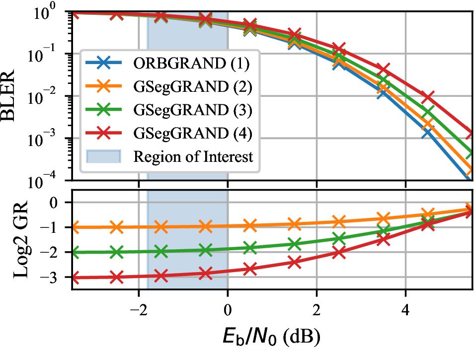
Fig. 10 shows the BLER and Log2 GR of a (32, 21) dRM code and marks the SNR range of the corresponding TPC’s waterfall region7 (see Fig. 12 for decoding results of the corresponding TPC). In the TPC’s waterfall region, GSegGRAND achieves almost maximal guesswork reduction for the corresponding component code.
5.3 Decoding of Turbo Product Codes↩︎
We compare TPC decoding with GSegGRAND and ORBGRAND component code decoding. For all TPCs, we use the following decoding parameters as in the original SOGRAND paper[29]: damping factor \(\alpha = 0.5\) and list size \(N_{\mathcal{L}} = 4\). List decoding terminates when the estimated list error is below \(T = \num{e-5}\) or if 10000 guesses are reached. To specify a TPC’s parameters and dimensions, we denote a TPC based on an \((n,k)\) component code \(\mathcal{C}_\text{c}\) as “\((n^2, k^2) = (n,k)^2 \; \mathcal{C}_\text{c}\) TPC” in the figures captions.
Fig. 11 shows the decoding performance for a \((32, 21)^2\) dRM TPC, which outperformed its corresponding 5G LDPC code under SOGRAND decoding with ORBGRAND [29].
![Figure 11: Decoding performance and guesswork for the (1024, 441) = (32, 21)^2 dRM TPC. (The LDPC BLER curve is from [29].)](/article/2607.12147/img/tcp_dRM32_21_new_small.png "fig:")
The plot shows the TPC’s BLER performance, the Log2 GR, and the average number of decoding iterations. The Log2 GR is calculated from the total number of guesses, counting the guesses of all component decoders over all iterations until TPC decoding terminates. The number of decoding iterations counts the number of full decoding iterations before termination.
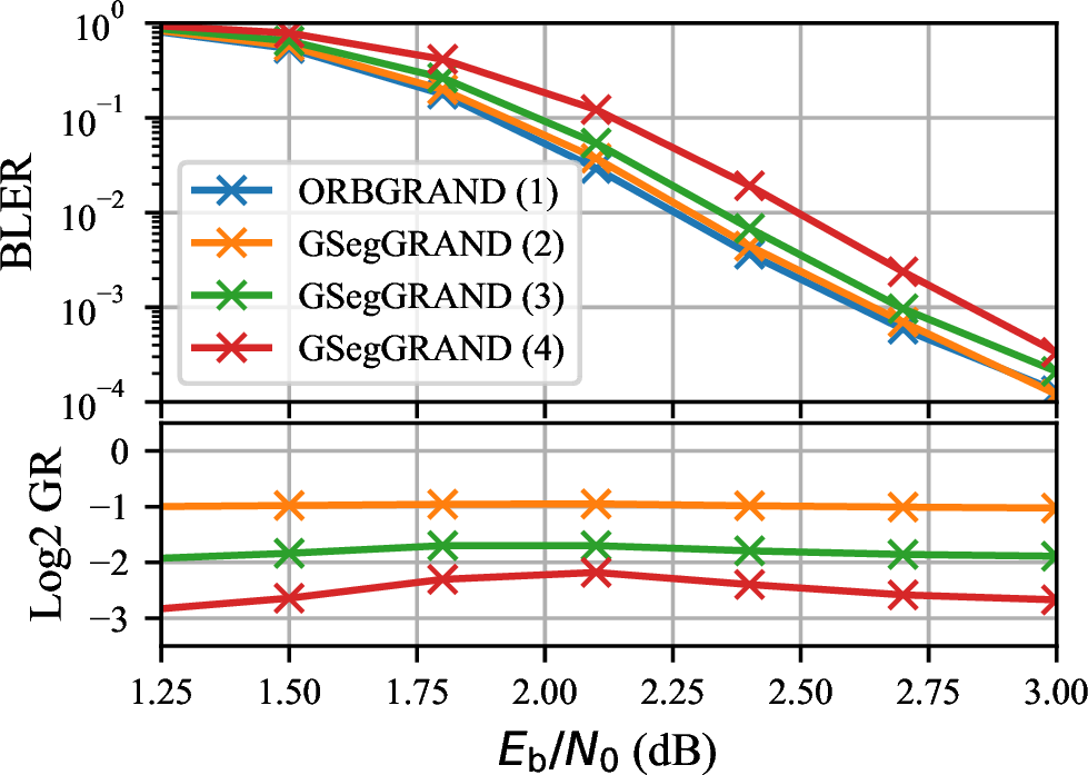
Although (32, 21) dRM component decoding experienced small BLER performance losses with GSegGRAND in Fig. 10, GSegGRAND with 2 and 4 segments achieves ORBGRAND’s TPC decoding performance with almost the same average number of decoding iterations while reducing the guesswork by \(2\) and \(4\) across the SNR range. The component decoder loss is most likely mitigated by the TPC list decoding, which filters out small guessing order degradations. GSegGRAND with 8 segments reduces the guesswork further while experiencing a BLER performance loss of less than 0.2 dB. In this case, each segment only contains 4 bit positions, resulting in a higher variance of the reliabilities per segment. TPC decoding with GSegGRAND therefore outperforms the corresponding LDPC code under BP decoding for 2 and 4 segments. To demonstrate generality, we also evaluated an (1024, 676) TPC with a (32,26) eBCH component code, for which we observe similar results, as shown in Fig. 12.
5.4 Soft-Output Calculation for Constrained Guessing↩︎
To show the importance of the SO calculation with conditioned noise effect probabilities 15 in Sec. 4 for turbo product decoding, we compared its performance against the original SO computation in 5 based on unconditional noise effect probabilities. We refer to the unconditioned and conditioned SO computation as (SO) and (SO+), respectively.
We first compare how well the SO of GSegGRAND (SO) and (SO+) matches ORBGRAND’s SO without constrained guessing, which is our baseline in this section. To do so, we transmit \(10000\) (32, 26) eBCH codewords over a BI-AWGN channel with \(E_\textrm{b} / N_0= \SI{3}{\dB}\)8 and SISO-decode the received signals with ORBGRAND and GSegGRAND yielding an LLR pair \((\ell_{\text{ORB},i}, \ell_{\text{GSeg},i})\) for each bit \(i\). Figure 13 shows the pairs as a scatter plot with (SO) (left) and (SO+) (right) computation.
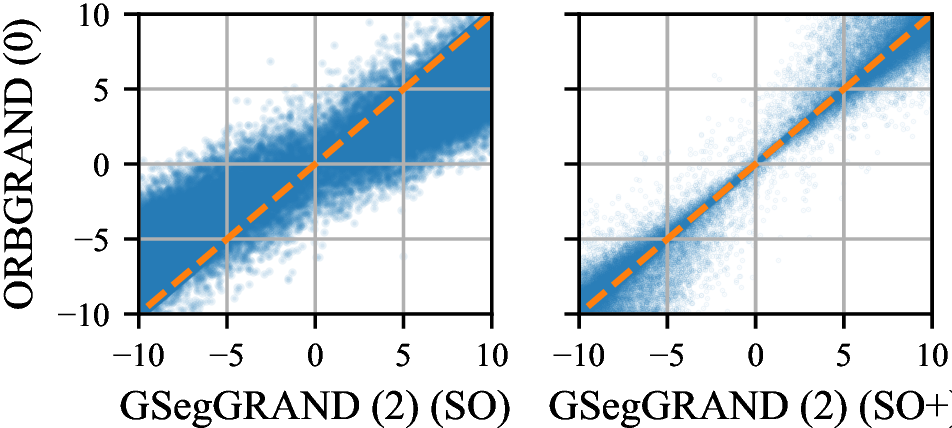
GSegGRAND’s SO closely match with ORBGRAND’s, i.e., \(\ell_{\text{ORB},i} \approx \ell_{\text{GSeg},i}\), when the scatter points lie on the \(x=y\) diagonal (orange dashed line). There is a significant discrepancy between GSegGRAND with the unconditioned SO calculation and ORBGRAND: when ORBGRAND outputs LLRs with magnitude smaller \(5\), the unconditioned SO even frequently produces LLRs with opposite sign. On the other side, GSegGRAND (SO+) almost always produces LLRs of the same sign as ORBGRAND and matches ORBGRAND’s LLRs closely at low LLRs.
Figure 14 shows how the (SO) and (SO+) computation affect the turbo product decoding performance for the \((32, 21)^2\) dRM TPC and \((32, 26)^2\) eBCH TPC.
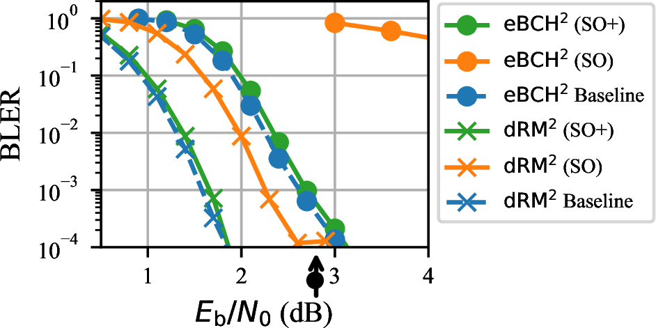
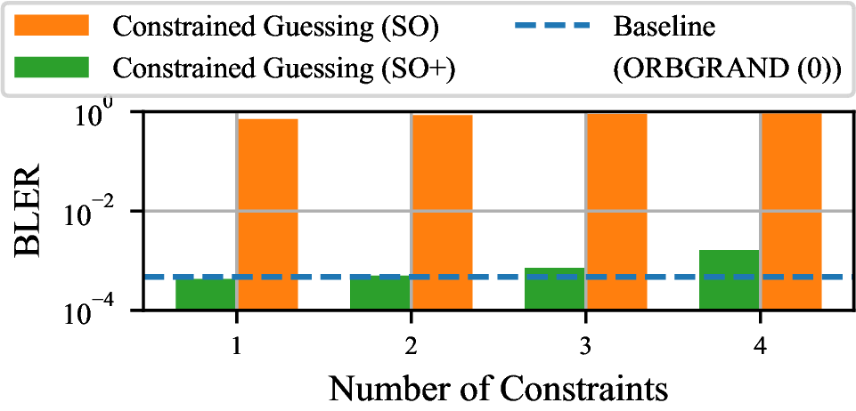
With the proposed SO calculation (SO+), turbo product decoding with GSegGRAND (3) performs close to the baseline ORBGRAND (0) (dashed blue). (SO+) gains up to 0.7 dB over (SO) for the \((32, 21)^2\) dRM TPC and enables efficient decoding for the \((32, 26)^2\) eBCH TPC, which otherwise experiences a high error floor with (SO) and constrained guessing. This behavior is consistent for constrained guessing across the number of constraints where Fig. 15 shows the BLER performance of the \((32, 26)^2\) eBCH TPC in the waterfall region (black vertical dashed line in Fig. 14) for a varying number of constraints. In this plot, 2-4 constraints correspond GSegGRAND and one constraint corresponds to ORBGRAND (1), which skips noise effects of incorrect parity for even codes (see Sec. 4). Note that not only GSegGRAND benefits from (SO+) but also ORBGRAND (1) if it skips noise effects of incorrect parity for even codes (see Sec. 4), requires (SO+).
6 Conclusion↩︎
In this paper, we presented GSegGRAND, a novel generalization of Segmented GRAND that efficiently incorporates multiple parity check constraints during guessing. The underlying parity check matrix structure is designed such that arbitrary linear codes can be systematically transformed into it, facilitating the extraction of multiple constraints. For iterative TPCs decoding, we demonstrate that the unmodified SOGRAND SO computation becomes inaccurate under constrained guessing, and derive a novel, accurate SO formula for GSegGRAND and Segmented GRAND. By explicitly incorporating the constraints in the SO computation, GSegGRAND achieves guesswork reduction of up to \(88 \%\) under turbo product decoding while maintaining near ORBGRAND BLER performance. While we focus here on the practical case of soft-input decoding, the balanced tree transformation provides a general framework for GRAND guesswork reduction that is applicable to various applications, such as hard-decision decoding. Since hard-decision decoding has no discrepancy between 3 and 11 , GSegGRAND can reduce guesswork without sacrificing BLER. Our evaluation demonstrates that GSegGRAND is a promising candidate for low-latency and high-performance decoding in future communication systems, offering a systematic path to GRAND guesswork reduction across a broad class of linear codes.
References↩︎
L. Rapp and M. Médard are with the Research Laboratory for Electronics, Massachusetts Institute of Technology, Cambridge, MA 02139 USA (e-mail: rappl@mit.edu; medard@mit.edu).↩︎
J. Feng and K. R. Duffy are with the Dept. of Mathematics and Dept. of ECE, Northeastern University, Boston, MA 02115 USA (e-mail: feng.ji@northeastern.edu; k.duffy@northeastern.edu).↩︎
This work was supported by the Defense Advanced Research Projects Agency (DARPA) under Grant HR00112120008.↩︎
Note that a full sorting is not necessary as ORBGRAND can start decoding once the least reliable bits are identified, and incrementally sorts additional values until a valid codeword is found [9].↩︎
Concretely, we converted the \(E_\textrm{b} / N_0\) range of the TPC’s waterfall region from Fig. 11 into a \(E_\textrm{s} / N_0\) range and back into the corresponding \(E_\textrm{b} / N_0\) range of the component code.↩︎
Turbo product decoding with ORBGRAND achieves a target BLER of × 10−4 at this operational point.↩︎