Benchmarking Sensor Robustness in Plasma Diagnostic Models:
A Systematic Evaluation on TokaMark
July 05, 2026
Abstract
Plasma diagnostic models for tokamak fusion devices are almost universally evaluated on clean, complete sensor data. In practice, fusion diagnostics fail regularly: acquisition systems start late, individual sensors die, and signal dropouts cluster precisely when a plasma disruption is approaching. We present the first systematic robustness benchmark for plasma diagnostic ML using the TokaMark dataset of 11,573 MAST shots [1], evaluating XGBoost, LSTM, Transformer, and the TokaMark CNN baseline across six physically-grounded failure scenarios and three imputation strategies. We introduce the Robustness Score (RS) for standardized cross-architecture comparison. Our central finding is that disruption-proximate sensor failure—corruption injected in the final window timesteps—collapses sequence model performance (LSTM \(+212\%\) NRMSE) while a statistical feature model remains comparatively stable (XGBoost \(+37\%\)). Forward-fill imputation eliminates nearly all degradation from random dropout for sequence models (LSTM \(+57\% \to {\sim}0\%\)), but offers little help when the end of the window is corrupted. Shot-level alarm evaluation using ground-truth disruption timestamps reveals that LSTM alarm detection collapses to TPR = 0.00 under proximate sensor failure, while mean-fill imputation recovers it to TPR = 1.00, a reversal of the pattern observed in NRMSE. Plasma current emerges as the single most critical diagnostic across all architectures (\(+73\%\) to \(+140\%\) upon removal). Code, data, and trained checkpoints are available at https://github.com/Neerav-Gupta/tokamark-robustness.
-2.3ex 1ex Introduction
-2ex 0.75ex Nuclear Fusion and Tokamaks
Nuclear fusion has long been considered one of the most compelling paths toward clean, abundant energy. Where fission splits heavy atoms and leaves behind radioactive byproducts, fusion joins light hydrogen isotopes (deuterium and tritium) and releases substantially more energy per reaction, with helium as the main product [2]. The fuel supply is effectively inexhaustible: deuterium is extracted from seawater, and tritium can be bred from lithium. A working fusion power plant would emit no carbon, produce no long-lived radioactive waste, and carry no risk of a runaway reaction [3].
The central difficulty is confining the fuel long enough for fusion to occur. The reaction requires temperatures above 100 million degrees Celsius, hotter than the core of the Sun, at which hydrogen exists as a plasma that would instantly destroy any material it contacted. Magnetic confinement fusion (MCF) handles this by using carefully shaped magnetic fields to keep the plasma suspended away from reactor walls [2]. Among MCF concepts, the tokamak has proven the most successful, and ITER, now under construction in southern France at an estimated cost of $22 billion, is the international experiment intended to demonstrate net energy gain from fusion for the first time [4].
-2ex 0.75ex Disruptions: The Critical Safety Challenge
A plasma disruption is a sudden, uncontrolled loss of plasma confinement: within milliseconds, the thermal and magnetic energy stored in the plasma dumps into the reactor walls [5]. De Vries et al. [5] catalogued disruptions at JET, the Joint European Torus and the world’s largest operating tokamak, finding they occur in roughly 3–4% of routine plasma shots, with higher rates under demanding operating conditions. At the scale of ITER or a commercial plant, each disruption inflicts heat loads, electromagnetic impulses, and runaway electron beams capable of permanently damaging the first wall, magnets, and structural components [4].
The economic stakes are considerable. Maris et al. [6] showed that even moderate disruption rates push up the levelized cost of electricity enough to threaten the commercial viability of fusion energy. The practical response is early disruption prediction: if a machine’s control system receives even 50–100 milliseconds of warning, it can gracefully terminate the plasma before damage occurs [7]. Reliable, real-time prediction is therefore not merely a performance goal; it is a safety requirement for any reactor-class device.
-2ex 0.75ex AI for Plasma Prediction
Plasma physics is complex and the diagnostic environment is demanding, which together create a strong case for data-driven methods. Fusion diagnostics cover magnetics, optical emission, X-ray cameras, microwave interferometry, and more, spanning sampling rates from 200 Hz to 500 kHz and producing inherently multi-modal, asynchronous, and noisy data [8]. Machine learning models can fuse these heterogeneous streams, respond in real time, and capture nonlinear dynamics without requiring explicit physical parameterization [9].
Progress has been rapid. Kates-Harbeck et al. [7] showed that deep recurrent networks trained on raw diagnostic time series could predict disruptions across JET and DIII-D with strong performance. Vega et al. [10] took this further, deploying an AI-based disruption prediction system at JET that matched or outperformed existing physics-based predictors. Churchill et al. [11] demonstrated that convolutional networks operating directly on high-resolution diagnostics could reliably identify pre-disruption states on DIII-D. More recently, foundation model approaches have been proposed as a path toward general-purpose plasma representations: Churchill [9] laid out the theoretical case, and TokaMind [12] delivered the first open-source multi-modal transformer trained on MAST data and benchmarked on TokaMark tasks.
-2ex 0.75ex The Missing Robustness Problem
Despite this progress, almost every published evaluation rests on the same unstated assumption: that sensor data arriving at inference time is complete and clean. In practice this assumption regularly fails. Acquisition systems start late, producing front-loaded gaps that cover 10–16% of signal history. Individual sensors fail mid-shot due to heat damage and electromagnetic interference. And these failures are not uniformly distributed in time; they tend to occur precisely when the plasma is most unstable and prediction is most critical. A disruption produces intense heat loads and electromagnetic transients that actively degrade sensor performance in the moments leading up to the event [1], [13].
TokaMark [1] acknowledges this directly, identifying robustness to incomplete state information as one of its four core benchmark dimensions and noting that signals “may be absent for a given shot due to hardware issues” or “contain missing time segments due to limited acquisition windows or diagnostic failures.” Yet no evaluation of this dimension appears anywhere in the TokaMark paper, and no prior work has systematically studied how plasma diagnostic models degrade under controlled sensor failure.
This paper addresses that gap directly. Our contributions are:
Natural missingness characterization. We stream 300 MAST shots from FAIR-MAST and characterize the real NaN structure of each diagnostic category, finding that failures are front-loaded and category-correlated, directly informing our scenario design.
Six physically-grounded failure scenarios. We implement random dropout, channel ablation, temporal gaps (front, random, pre-event), correlated diagnostic group failure, and disruption-proximate failure. The last scenario, to our knowledge, has not been evaluated in any prior work.
Cross-architecture robustness benchmark. We evaluate XGBoost, LSTM, Transformer, and the TokaMark CNN baseline on Task 4-4 under all six scenarios, and introduce the Robustness Score (RS) as a standardized metric we encourage the community to adopt.
Shot-level alarm evaluation. Using ground-truth disruption timestamps (
t_cut) from FAIR-MAST, we compute true positive rate (TPR) and mean warning time (MWT) for each model under clean and corrupted conditions.Mitigation strategy evaluation. We evaluate zero-fill, mean-fill, and forward-fill imputation across all scenarios for both NRMSE and shot-level alarm metrics, revealing that the optimal strategy differs between the two evaluation regimes.
-2.3ex 1ex Related Work
0.0.0.1 TokaMark and FAIR-MAST.
Rousseau et al. [1] introduced TokaMark as the first large-scale, openly available benchmark for AI models on real fusion data, defining 14 tasks across four groups over an 80/10/10 shot-level split drawn from the FAIR-MAST dataset [13], [14]. Their CNN baseline reaches NRMSE 0.429 on Task 4-4 using the full 9,270-shot training set. TokaMark lists robustness to incomplete state information as one of its core evaluation dimensions but stops short of actually evaluating it. The present work takes up that thread.
0.0.0.2 Disruption prediction.
Machine learning for disruption prediction has attracted sustained effort over the past decade. Kates-Harbeck et al. [7] established that cross-device deep learning was feasible on JET and DIII-D data. Vega et al. [10] brought an AI predictor into real-time operation at JET. Churchill et al. [11] explored raw high-resolution diagnostic inputs on DIII-D. Aymerich et al. [15] incorporated spatiotemporal profile structure at JET, and Guo et al. [16] applied similar approaches to EAST. Every one of these studies assumes complete, clean sensor availability at inference time, an assumption our work directly interrogates.
0.0.0.3 Disruption alarm systems.
Rea et al. [17] deployed a real-time ML disruption predictor on DIII-D, establishing the standard per-shot alarm metric framework (true positive rate, false alarm rate, warning time) used in the field. Saperstein et al. [18] designed an off-normal warning system for SPARC. Ai et al. [19] developed adaptive anomaly detection for disruption prediction from first discharge. Spangher et al. [20] introduced DisruptionBench as a systematic evaluation framework. All of these works assume complete sensor availability; our work evaluates what happens when that assumption fails.
0.0.0.4 Autoregressive plasma state forecasting.
Several recent works use autoregressive sequence models for full-shot plasma state prediction in reactor control contexts. Char et al. [21] demonstrated deep recurrent networks for full-shot prediction on DIII-D. Wang et al. [22] introduced the POPSIM framework for autoregressive plasma state forecasting. Jalalvand et al. [23] applied multimodal super-resolution to discover hidden physics in fusion plasmas. These works share our sequence-based modeling spirit but focus on clean-data prediction rather than robustness under sensor failure.
0.0.0.5 Missing data in tokamak ML.
Two prior works come closest to our setting. Chandrasekaran et al. [24] tested CatBoost on 187 GOLEM shots with missing values, tracing most degradation to interferometer outages. Yang et al. [25] tackled the related problem of channels that are entirely absent when a model is deployed on a new device, proposing learned pseudo-data placeholders for the HL-3 disruption predictor. Both studies are narrower than ours in scope: we evaluate four model architectures across six distinct failure modes at multiple severities, with three imputation strategies, and introduce the first standardized robustness metric for this class of problem.
0.0.0.6 Data augmentation for cross-device generalization.
Chayapathy et al. [26] developed time-series viewmakers, learned augmentations combining jittering, slicing, and temporal warping, to improve disruption prediction robustness when transferring between tokamak devices via the DisruptionBench framework. That work is concerned with distribution shift across machines, not sensor failure during a single inference, and is complementary to ours.
0.0.0.7 Foundation models for fusion.
TokaMind [12] is the first open-source multi-modal transformer foundation model for tokamak plasma dynamics, trained on MAST data. Churchill [9] made the broader case for foundation model approaches in fusion. Both acknowledge missing-channel handling as a real deployment challenge but do not quantify the resulting degradation, which is what we provide.
0.0.0.8 XGBoost for scientific time series.
Chen and Guestrin [27] designed XGBoost with a sparsity-aware split-finding algorithm that handles missing feature values natively without any imputation step. This makes it a natural comparison point for studying how architectural inductive bias shapes robustness in sequence-based deep learning models.
-2.3ex 1ex Background
-2ex 0.75ex The MAST Tokamak and FAIR-MAST
MAST was a spherical tokamak operated at Culham, UK by the UK Atomic Energy Authority from 1999 to 2013 [28], [29]. Over its lifetime it produced more than 30,000 plasma shots, each lasting roughly 2–3 seconds. Its compact spherical geometry distinguished it from conventional tokamaks and made it a particularly useful testbed for studying plasma dynamics and disruption physics relevant to future spherical power plant concepts [30].
FAIR-MAST [13], [14] makes diagnostic data from 11,573
shots across MAST’s final five experimental campaigns openly available in Zarr format via a public S3 endpoint. Each shot includes a ground-truth disruption timestamp (t_cut), the time at which plasma current quench occurs. TokaMark [1] draws on this data, selecting 39 signals and defining 14 prediction tasks with an 80/10/10 shot-level split: 9,270 training shots,
1,157 validation shots, and 1,146 test shots.
-2ex 0.75ex Task 4-4: Plasma Current Quench Prediction
Among TokaMark’s 14 tasks, we focus on Task 4-4: given 150 milliseconds of diagnostic history, predict the plasma current 100 milliseconds into the future. This is a non-Markovian autoregressive forecasting task; the full input history is needed, not just the current state [1]. It is also the most directly safety-relevant task in the benchmark, since plasma current quench is one of the clearest precursors of a full disruption, and any prediction system operating in a real device must handle it reliably.
The task takes 14 diagnostic input signals and 4 actuator signals as input, listed in Table 1. These span the full range of MAST diagnostic categories: flux loops and pickup coils in magnetics, interferometer and D-alpha in kinetics, soft X-ray in radiatives, and active coil currents, plus the four actuator channels encoding reference trajectories and fueling.
| Index | Signal | Category |
|---|---|---|
| 0 | interferometer-n_e_line | Kinetics |
| 1 | magnetics-ccbv_field | Magnetics |
| 2 | magnetics-obr_field | Magnetics |
| 3 | magnetics-obv_field | Magnetics |
| 4 | magnetics-omv_voltage | Magnetics |
| 5 | magnetics-cc_field | Magnetics |
| 6 | magnetics-saddle_voltage | Magnetics |
| 7 | magnetics-flux_loop_flux | Magnetics |
| 8 | pf_active-coil_current | Active coils |
| 9 | pf_active-solenoid_current | Active coils |
| 10 | soft_x_rays-cam_lower | Radiatives |
| 11 | soft_x_rays-cam_upper | Radiatives |
| 12 | spectrometer-dalpha_voltage | Kinetics |
| 13 | summary-ip | Plasma current |
| 14 | gas_injection-total_injected | Actuator |
| 15 | pulse_schedule-i_plasma | Actuator |
| 16 | pulse_schedule-n_e_line | Actuator |
| 17 | summary-power_nbi | Actuator |
-2ex 0.75ex Natural Missingness in MAST
To ground our corruption scenarios in real failure patterns rather than arbitrary assumptions, we streamed 300 shots from FAIR-MAST and measured the NaN structure of each diagnostic category. Table 2 summarizes the results. Two findings shape everything that follows.
Category-stratified missingness. Plasma current and coil currents are present in every shot (0% NaN across all 300), reflecting the engineering priority placed on these signals for real-time control. Kinetics diagnostics (interferometer and D-alpha) average 14–15% NaN per shot, caused by acquisition delays that consistently produce a front-loaded gap at the start of each shot.
Perfectly correlated failures. The NaN percentages for interferometer and D-alpha are identical to four decimal places in every sampled shot, a correlation of \(r = 1.000\). The two diagnostics share a single acquisition trigger: when that trigger fires late, both signals are simultaneously absent. This is not a statistical pattern but a hardware reality, and it directly motivates the correlated group failure scenario in Section [sec:sec:scenarios].
| Signal category | Mean | Max | Missing | Structure |
| NaN% | NaN% | shots | ||
| Magnetics (ip, coils) | 0.0 | 0.0 | 0/300 | Always present |
| Flux loops | 3.7 | 33.3 | 0/300 | Variable |
| Soft X-ray | 1.9 | 34.1 | 15/300 | Variable |
| D-alpha spectrometer | 14.4 | 42.5 | 7/300 | Front block |
| Interferometer | 15.0 | 42.5 | 23/300 | Front block |
-2.3ex 1ex Methodology
-2ex 0.75ex Model Architectures
We evaluate four architectures representing fundamentally different inductive biases for multivariate time-series prediction.
0.0.0.9 XGBoost [27].
Rather than operating on raw time series, we first compress each window into 142 summary statistics: 9 per input signal (mean, std, min, max, median, first value, last value, linear slope, and zero fraction across 14 input signals) and 4 per actuator signal (mean, std, first, last across 4 actuators). This discards all temporal structure but compactly captures the distributional properties of each signal. The XGBoost regressor uses 500 estimators, learning rate 0.05, max depth 6, subsample 0.8, colsample 0.8, and GPU histogram-based tree building with early stopping after 20 rounds of no improvement on validation NRMSE. Total split capacity: \(\sim\)500K decision tree nodes.
0.0.0.10 LSTM.
Each diagnostic signal is spatially averaged to a scalar time series and resampled to a fixed 600 timesteps by linear interpolation, yielding a \((600, 18)\) tensor input. A 2-layer LSTM (hidden size 128, dropout 0.2) processes this sequence and the final hidden state passes through a two-layer MLP (\(128 \to 64 \to 1\)) to produce the prediction. We train with Adam at learning rate \(10^{-3}\), ReduceLROnPlateau scheduling (patience 5, factor 0.5), gradient clipping at 1.0, and early stopping with patience 15. Total parameters: \(\sim\)430K.
0.0.0.11 Transformer.
The same \((600, 18)\) tensor is linearly projected into a 128-dimensional space, enhanced with sinusoidal positional encodings, and passed through a 3-layer Transformer encoder (4 attention heads, feedforward dimension 256, dropout 0.1). A global average pool over the time axis feeds the same MLP head (\(128 \to 64 \to 1\)). Training uses Adam with cosine annealing (\(T_\mathrm{max}=100\), \(\eta_\mathrm{min}=10^{-5}\)), gradient clipping at 1.0, and early stopping with patience 15. Total parameters: \(\sim\)310K.
0.0.0.12 CNN (TokaMark baseline).
We implement the multi-branch convolutional encoder described in Rousseau et al. [1], providing a direct comparison to the TokaMark-reported baseline. Each of the 18 input channels is processed by a dedicated 1D convolutional encoder (\(N=3\) layers, kernel \(K=3\), stride \(s=3\), padding \(p=1\), latent dimension \(D=16\)). The resulting per-channel latent vectors are concatenated and passed through a shared MLP backbone (\(64 \to 32 \to 16 \to 1\)). Training uses Adam at learning rate \(10^{-3}\), ReduceLROnPlateau scheduling (patience 5, factor 0.5), gradient clipping at 1.0, and early stopping with patience 15. Total parameters: \(\sim\)458K.
All four models are trained on 9,950 windows from 200 training shots and evaluated on 2,420 windows from 50 test shots, following TokaMark’s shot-level split. Hyperparameters are collected in Table 3.
| Hyperparameter | XGB | LSTM | Transf. | CNN |
|---|---|---|---|---|
| Optimizer | Hist/GPU | Adam | Adam | Adam |
| Learning rate | 0.05 | \(10^{-3}\) | \(5\!\times\!10^{-4}\) | \(10^{-3}\) |
| LR schedule | – | ReduceLRP | Cosine | ReduceLRP |
| Batch size | Full | 64 | 64 | 64 |
| Max epochs | 500 trees | 100 | 100 | 100 |
| Early stopping | 20 | 15 | 15 | 15 |
| Dropout | – | 0.2 | 0.1 | 0.1 |
| Grad clip | – | 1.0 | 1.0 | 1.0 |
| Parameters | \(\sim\)500K | \(\sim\)430K | \(\sim\)310K | \(\sim\)458K |
-2ex 0.75ex Model Pipeline
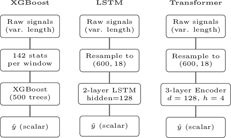
Figure 1 illustrates the three sequence modeling pipelines from raw diagnostic signals to prediction. The CNN uses the same \((600, 18)\) tensor representation as LSTM and Transformer but applies per-channel convolutional encoders rather than processing the full multivariate sequence directly.
-2ex 0.75ex Evaluation Metrics
0.0.0.13 NRMSE.
We measure window-level prediction quality using Normalized Root Mean Squared Error: \[\text{NRMSE} = \frac{\sqrt{\frac{1}{N}\sum_{i=1}^{N}(\hat{y}_i - y_i)^2}}{\sigma_y} \label{eq:nrmse}\tag{1}\] where \(\sigma_y\) is the standard deviation of the ground truth over the test set. An NRMSE of 1.0 means the model is no better than predicting the mean; values below 1.0 indicate genuine predictive value [1]. We compute NRMSE at the window level and average across all test windows. This differs from TokaMark’s full shot-level hierarchical aggregation protocol [1], so our absolute values should not be read as direct comparisons to TokaMark baselines.
0.0.0.14 Shot-level alarm metrics.
Following the disruption prediction literature [17], [20], we additionally compute
shot-level application metrics using ground-truth disruption timestamps (t_cut) from FAIR-MAST. An alarm is issued for a shot when the model’s predicted plasma current drops below a threshold fraction of the shot’s mean predicted current. The
threshold is optimized per model by sweeping \(\theta \in [0.05, 0.60]\) to maximize true positive rate (TPR). All 50 test shots disrupted (finite t_cut), so we report TPR and mean warning time (MWT, the mean
time between first alarm and t_cut); false alarm rate (FAR) cannot be computed without non-disruptive shots.
-2ex 0.75ex Robustness Score
To enable principled comparison across architectures and scenarios, we introduce the Robustness Score: \[\text{RS} = \frac{1}{|\mathcal{S}|} \sum_{s \in \mathcal{S}} \frac{\text{NRMSE}_\text{clean}}{\text{NRMSE}_s} \label{eq:rs}\tag{2}\] where \(\mathcal{S}\) is the full set of zero-fill corruption scenarios. RS \(= 1.0\) means corruption has no effect; values below 1.0 scale linearly with the degree of degradation. We encourage adoption of RS as a standard component of future plasma ML robustness evaluations.
-2ex 0.75ex Corruption Scenarios
We implement six failure scenarios, each physically grounded in real tokamak failure modes. All scenarios are applied to the test set only; all models are trained exclusively on clean data.
0.0.0.15 Scenario 1: Random dropout.
A randomly chosen fraction \(p \in \{0.10, 0.25, 0.50\}\) of all signal values is set to zero, modeling random digitizer glitches and transient sensor noise. The mask is applied only to positions that were already nonzero, preserving natural acquisition gaps.
0.0.0.16 Scenario 2: Channel ablation.
A randomly selected set of \(n \in \{1, 3, 6\}\) complete diagnostic channels is zeroed for the duration of the window, modeling a dead or physically disconnected sensor.
0.0.0.17 Scenario 3: Per-category channel importance.
Following the TokaMark signal taxonomy [1], we zero each of eight diagnostic categories in isolation (flux loops, pickup coils, saddle coils, Mirnov spectrograms, kinetics comprising interferometer and D-alpha, soft X-ray, active coils, and plasma current) to identify which signals each architecture actually relies on.
0.0.0.18 Scenario 4: Temporal gap.
A contiguous block covering fraction \(f \in \{0.20, 0.40, 0.60\}\) of the window is zeroed across all channels simultaneously. We test three positions: front (acquisition delays, consistent with our MAST characterization), random (mid-shot loss), and pre-event (the final \(f\) fraction, affecting the timesteps closest to the prediction horizon).
0.0.0.19 Scenario 5: Correlated diagnostic group failure.
Motivated directly by the \(r = 1.000\) NaN correlation we found in MAST data (Section [sec:sec:missingness]), we zero all channels belonging to a physically related group simultaneously: kinetics (interferometer and D-alpha), active magnetics (all pickup coil arrays), radiatives (both soft X-ray cameras), and Mirnov spectrograms.
0.0.0.20 Scenario 6: Disruption-proximate failure.
A gap of fraction \(f \in \{0.10, 0.25, 0.50\}\) is injected at the very end of the prediction window. This is the scenario with the most direct safety implications: the sensors most critical for detecting disruption precursors fail in the final moments before the event the model is trying to predict.
-2ex 0.75ex Mitigation Strategies
We evaluate three imputation strategies applied after corruption, using the corruption mask to restrict filling to artificially zeroed positions rather than natural zeros.
0.0.0.21 Zero-fill.
No imputation is performed; corrupted values stay at zero. This is the implicit behavior of TokaMark’s own preprocessing pipeline [1] and serves as the baseline.
0.0.0.22 Mean-fill.
Corrupted values are replaced with the per-channel mean from the training set.
0.0.0.23 Forward-fill.
The last valid observation before each gap is carried forward until valid data resumes. This mirrors how most industrial sensor systems behave when a reading is unavailable and is the most physically natural strategy for a real-time control context.
0.0.0.24 Implementation note.
For XGBoost, temporal gap and dropout corruption are implemented as feature-level proxies (corrupting the trajectory statistics most sensitive to each gap position: first value, last value, and slope) rather than direct time-series masking used for LSTM, Transformer, and CNN. XGBoost temporal gap results are therefore conservative estimates of the true effect.
-2.3ex 1ex Results
-2ex 0.75ex Clean-Data Baselines
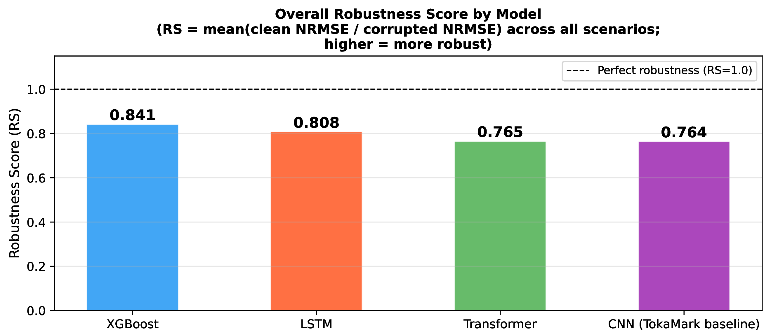
Table 4 reports clean-data NRMSE and Robustness Scores. The Transformer achieves the best prediction accuracy on clean data (NRMSE 0.470) but also the lowest robustness score (RS 0.765). XGBoost sits at the other end: slightly worse clean NRMSE, highest RS (0.841). The CNN achieves clean NRMSE 0.528 and RS 0.764, nearly identical to the Transformer, suggesting that multi-branch convolutional processing and global attention reach similar overall robustness despite very different inductive biases. This tradeoff between accuracy and robustness recurs throughout the results and has direct architectural implications.
Our clean NRMSE values sit above the TokaMark CNN baseline of 0.429 [1], which trains on the full 9,270-shot dataset compared to our 200 shots. The gap is expected and does not affect the validity of our robustness comparisons: relative degradation patterns are determined by architecture, not by clean-data starting point.
| Model | Clean NRMSE | RS |
|---|---|---|
| XGBoost | 0.494 | 0.841 |
| LSTM | 0.496 | 0.808 |
| Transformer | 0.470 | 0.765 |
| CNN (TokaMark baseline) | 0.528 | 0.764 |
-2ex 0.75ex Random Dropout
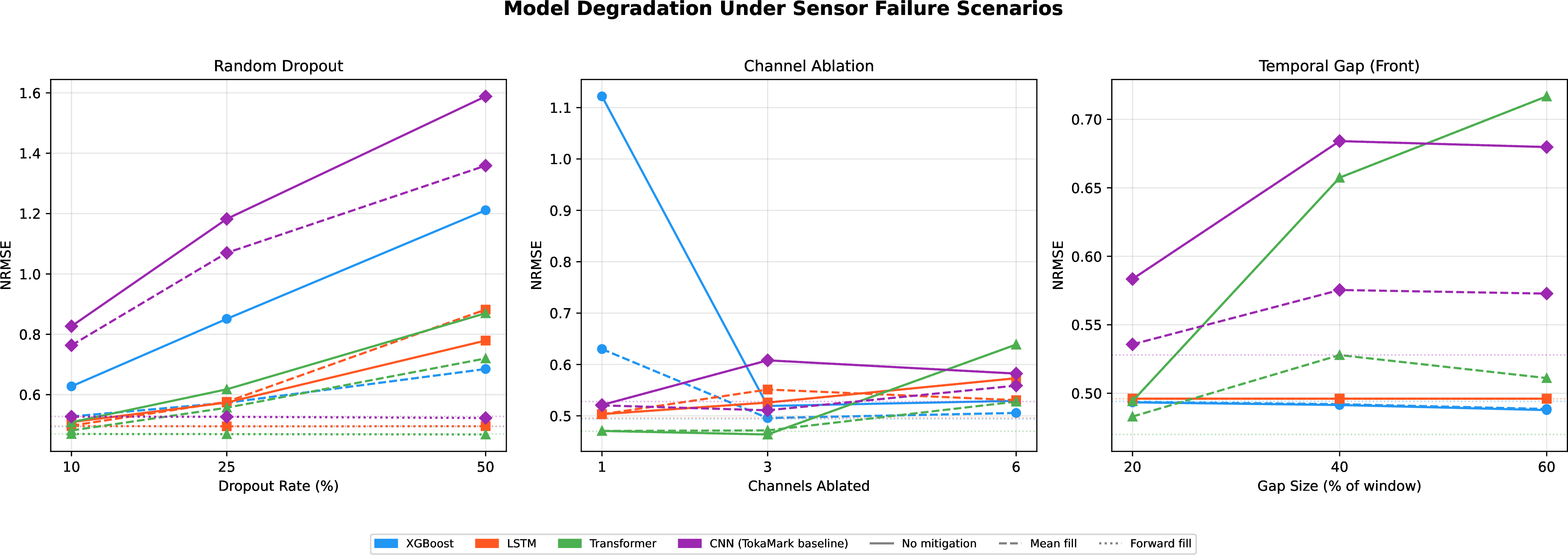
Figure 2 (left) traces NRMSE as dropout rate increases. XGBoost degrades the most under zero-fill, reaching \(+145\%\) at \(50\%\) dropout, as the statistical features that aggregate over the whole window are directly disrupted when many individual values are zeroed. LSTM and Transformer are less sensitive at \(+57\%\) and \(+85\%\) respectively. The CNN degrades most severely of all sequence models (\(+201\%\) at \(50\%\) dropout), as its per-channel statistical encoders are similarly sensitive to value corruption as XGBoost’s features.
Forward-fill essentially solves the dropout problem for sequence models. At \(50\%\) dropout, LSTM with forward-fill degrades by \({\sim}0\%\) and Transformer by \(-0.4\%\), both within measurement noise of their clean baselines. The reason is straightforward: forward fill converts a randomly damaged signal into a piecewise-constant one, and the models have seen signals with similar step-function character in training. XGBoost recovers only partially under mean-fill (\(+39\%\) at \(50\%\)), since imputing the mean into a feature vector that was computed from corrupted values is an imperfect fix.
-2ex 0.75ex Channel Ablation and Signal Importance
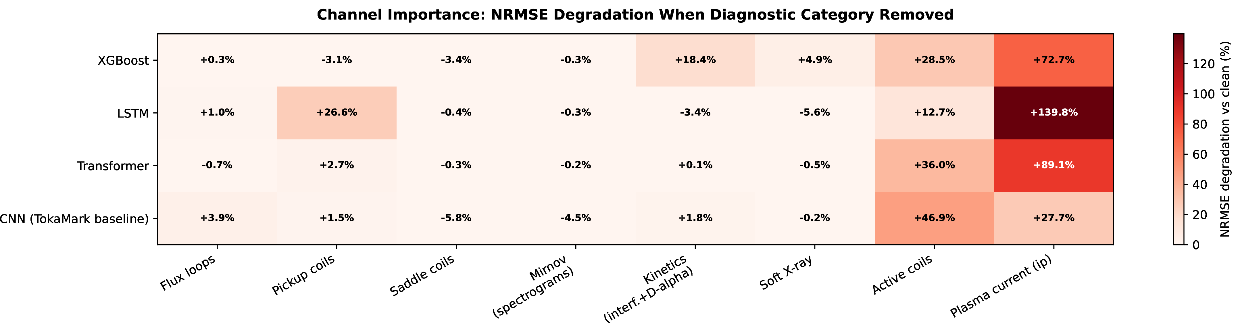
Figure 2 (center) shows overall degradation under channel ablation, while the per-category channel importance heatmap (Figure 3) shows a sharp hierarchy. Plasma current
(summary-ip) is dominant: removing it degrades LSTM by \(+139.8\%\), Transformer by \(+89.1\%\), XGBoost by \(+72.7\%\), and CNN by \(+27.7\%\). This is not surprising; plasma current is both the primary controlled variable in a tokamak discharge and the direct output of the task. The magnitude confirms that no architecture has found a substitute proxy.
Active coil currents are the next most important (Transformer \(+36.0\%\), XGBoost \(+28.5\%\), CNN \(+46.9\%\)), as they encode the machine’s immediate
control intent. CNN is the most sensitive architecture to active coil removal, reflecting its per-channel encoder design which cannot share information across channels in the encoding stage.
What is more interesting is what is not important. Kinetics (interferometer and D-alpha) and soft X-ray radiatives, the categories with the highest natural missingness in real MAST data, cause minimal degradation when removed (under \(+20\%\) for all models). The parsimonious explanation is that all four models have developed compensatory representations for these signals during training, precisely because they were frequently absent. A model that trains on 14–15% NaN rates learns, in effect, to treat those channels as optional.
-2ex 0.75ex Temporal Gap and Disruption-Proximate Failure
Figure 5 isolates the three temporal gap variants and reveals a stark asymmetry.
0.0.0.25 Front gap.
Removing the first 20–60% of the window barely affects LSTM (\(+0.0\%\) at \(60\%\) gap) or XGBoost (\(-1.3\%\) at \(60\%\) gap). This makes physical sense: the front of a MAST shot covers the pre-plasma ramp-up, which carries little information about the flat-top state being predicted. The Transformer is more affected (\(+52.5\%\) at \(60\%\) gap), consistent with its global attention mechanism treating all timesteps as equally informative rather than weighting recent timesteps more heavily. The CNN shows moderate sensitivity (\(+10.5\%\) to \(+28.8\%\)) due to its convolutional receptive field spanning the full window.
0.0.0.26 Proximate and pre-event failure.
Removing the final portion of the window is catastrophic for sequence models. LSTM hits \(+212\%\) NRMSE at the first tested severity (\(20\%\) gap) and stays there regardless of how large the gap grows, a hard performance ceiling indicating that the last few timesteps are irreplaceable for its predictions. This is the most concerning finding in the paper: the timesteps LSTM depends on most are precisely those most likely to be lost as a real disruption approaches. The Transformer degrades more gradually with gap size (\(+143\%\) at \(20\%\), \(+205\%\) at \(60\%\)), suggesting its distributed attention across the full sequence provides partial protection. The CNN degrades more gradually than LSTM (\(+67.7\%\) to \(+167.7\%\)) due to its convolutional pooling over the full sequence. XGBoost degrades moderately (\(+8\%\) to \(+37\%\)) because trajectory statistics like slope and last value are only partially sensitive to end-of-window corruption.
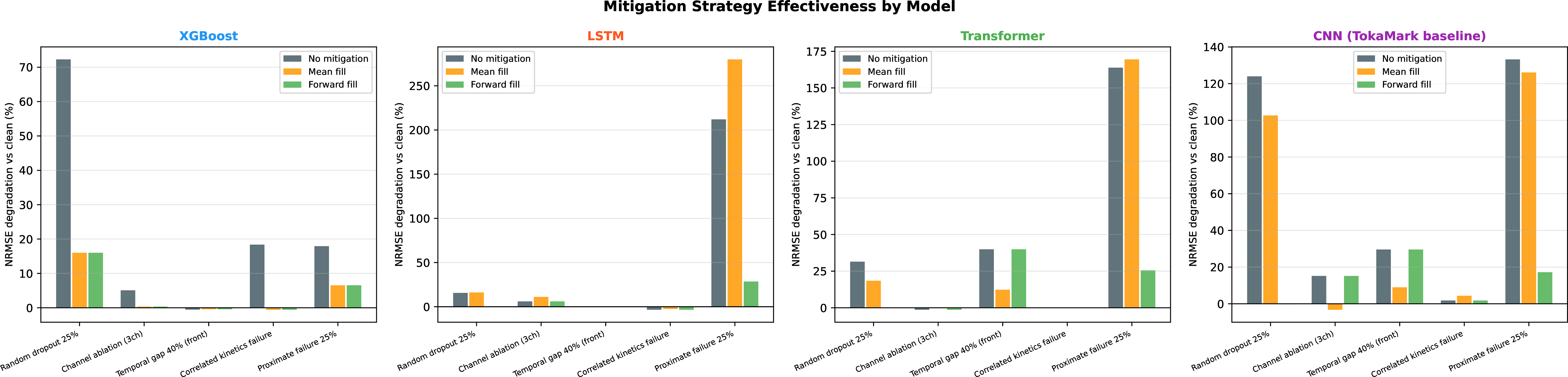
Forward fill offers partial recovery at low proximate gap severity (LSTM \(20\%\): \(+212\% \to +15\%\)) but cannot recover at higher severities. The reason is fundamental: imputing earlier values forward cannot reconstruct the genuinely new information that the final timesteps would have contained.
-2ex 0.75ex Correlated Diagnostic Group Failure
When entire diagnostic groups are removed simultaneously (Figure 4), a different pattern emerges. LSTM degrades most when active magnetics fail (\(+26.2\%\)) but is actually less affected by kinetics failure than XGBoost, consistent with the implicit compensation it has developed for kinetics dropouts during training. XGBoost suffers more under kinetics (\(+18.4\%\)) and radiatives (\(+20.2\%\)) removal, suggesting that statistical features of those signals carry weight in its predictions that its learned representations cannot easily replace. The CNN and Transformer show minimal degradation under all correlated group failures, with most values near or below zero, indicating strong implicit redundancy.
Mirnov spectrogram failure causes negligible degradation in all four models (under \(+1\%\)). Mirnov coils detect MHD instabilities that typically precede locked modes and disruptions, but those instability signatures may not be consistently present within the 150ms prediction window in this dataset, leaving the models with little reason to rely on them.
-2ex 0.75ex Mitigation Effectiveness
Figure 6 compares the three strategies across five representative scenarios. Forward fill leads for dropout and temporal gap, cutting LSTM \(50\%\)-dropout degradation from \(+57\%\) to near zero and Transformer \(50\%\)-dropout from \(+85\%\) to near zero.
For disruption-proximate failure the NRMSE picture reverses. At \(50\%\) proximate gap, mean fill makes LSTM worse (NRMSE rises from \(1.55\) to \(1.88\)) rather than better: substituting the channel mean into the prediction-critical final timesteps pushes the model toward an incorrect prior exactly where it needs real signal. Forward fill provides meaningful recovery only at the lowest severity (\(10\%\) proximate gap, LSTM: \(+212\% \to +1.7\%\)) and loses its effectiveness as the corrupted region grows. No simple imputation strategy resolves the fundamental problem that the information lost during disruption-proximate failure cannot be reconstructed from earlier observations when evaluated by NRMSE. However, the shot-level alarm perspective tells a different story (Section [sec:sec:alarm]).
-2ex 0.75ex Shot-Level Alarm Metrics
To address the gap between window-level ML metrics and deployment-relevant application metrics [17], [20], we compute shot-level disruption alarm metrics using the ground-truth t_cut disruption timestamps from FAIR-MAST.
0.0.0.27 Clean-data alarm performance.
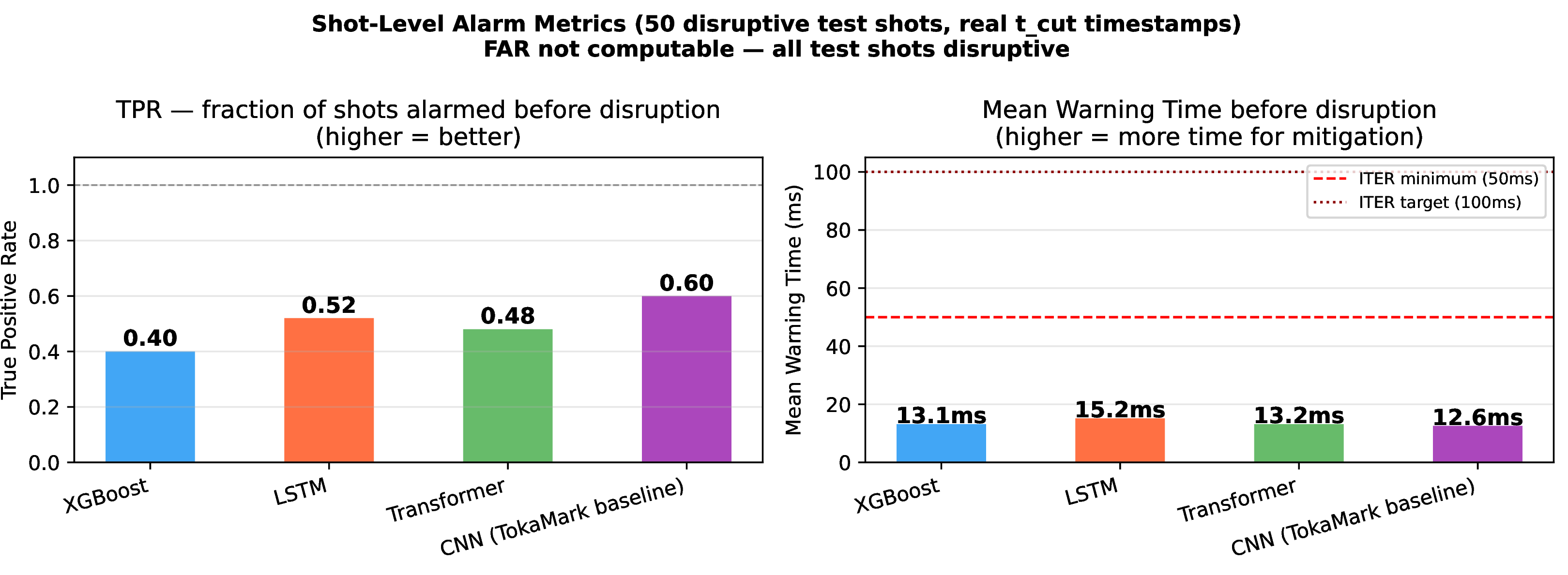
Table 5 reports results on clean data. CNN achieves the highest TPR (0.60), correctly alarming on 30 of 50 disruptive shots before disruption. Mean warning times of 12–15ms fall substantially short of the 50–100ms required for safe shutdown on ITER-class devices [7], highlighting the gap between current forecasting capability and operational requirements (Figure 8).
| Model | TPR | MWT (ms) |
|---|---|---|
| XGBoost | 0.40 | 13.1 |
| LSTM | 0.52 | 15.2 |
| Transformer | 0.48 | 13.2 |
| CNN (TokaMark baseline) | 0.60 | 12.6 |
0.0.0.28 Alarm performance under sensor failure.
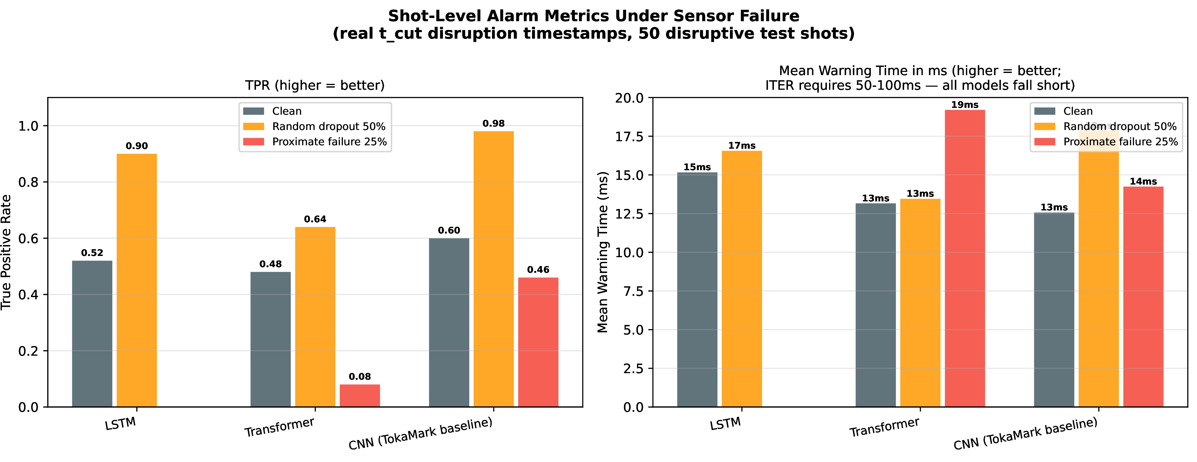
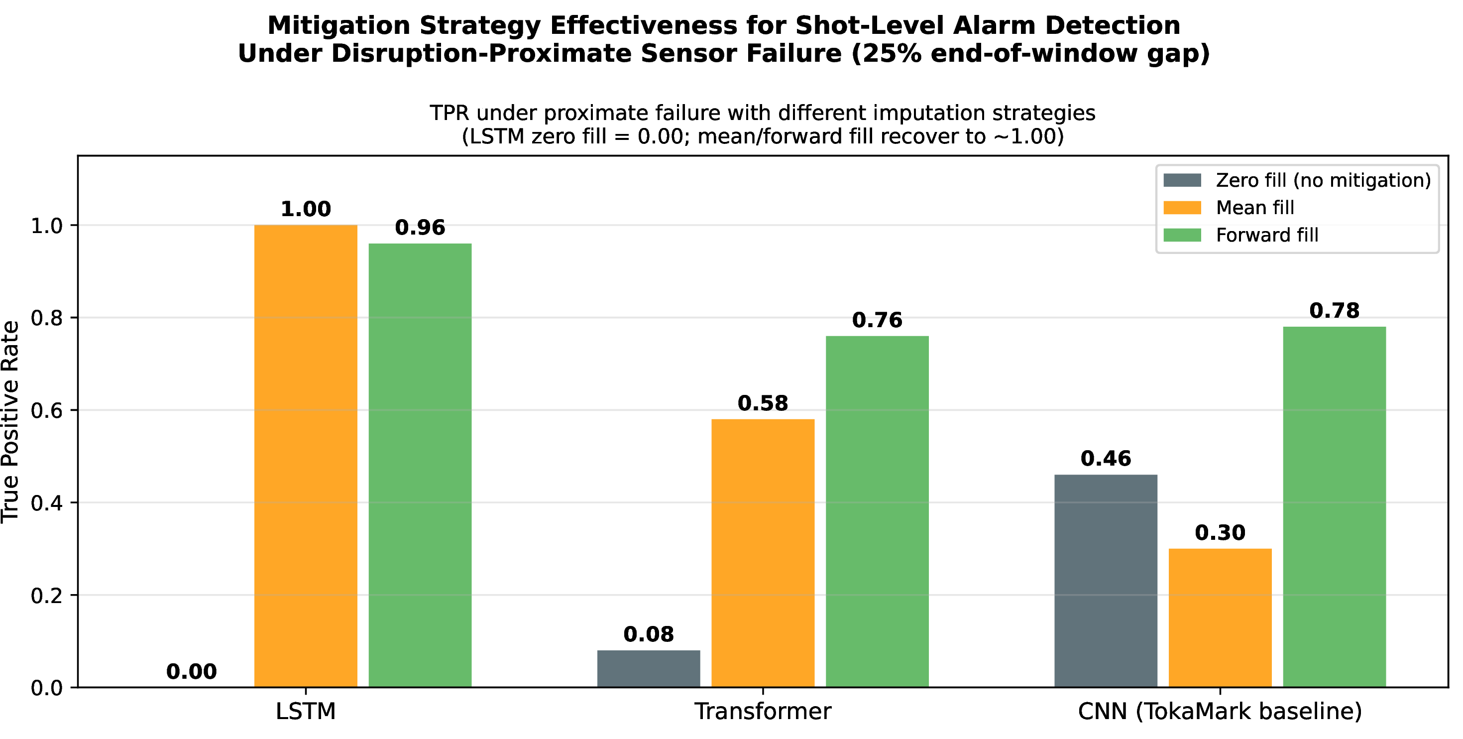
Figure 9 shows how TPR changes under two representative failure scenarios. Under 50% random dropout, all models maintain or increase TPR; the noise introduced by dropout creates spurious current drops that trigger alarms, coincidentally increasing detection rate. Under 25% proximate failure, the pattern reverses dramatically: LSTM TPR collapses from 0.52 to 0.00, Transformer drops to 0.08, and CNN drops to 0.46. When the sensors fail near the disruption, LSTM fails to alarm on every single test shot.
0.0.0.29 Mitigation for alarm detection.
Figure 10 reveals a striking and important result: the optimal mitigation strategy for alarm detection under proximate failure is the opposite of what NRMSE suggests. Under zero-fill, LSTM TPR = 0.00. Under mean-fill, LSTM TPR recovers to 1.00, with all 50 disruptive shots correctly alarmed. Forward fill also recovers strongly (TPR = 0.96). This reversal occurs because imputation prevents the artificial zeros from masking the current drop signal in the final timesteps, allowing the threshold alarm to fire correctly. For CNN, forward fill is preferable (TPR = 0.78 vs mean-fill TPR = 0.30), while for Transformer, forward fill also leads (TPR = 0.76 vs mean-fill TPR = 0.58).
The practical implication is significant: the incorrect prior that makes mean fill harmful for NRMSE prediction is precisely what makes it useful for alarm detection under proximate failure. Any fusion ML deployment system should evaluate mitigation strategies separately for prediction accuracy and alarm reliability.
-2.3ex 1ex Discussion
-2ex 0.75ex Architectural Inductive Bias and Robustness
The pattern across all results can be traced to a single underlying difference in how each model treats its input. XGBoost aggregates each signal into a handful of statistics before making any prediction; corrupting individual timesteps shifts those statistics by a bounded amount and the model’s predictions change proportionally. This is not a surprising property; Chen and Guestrin [27] designed XGBoost’s sparsity-aware split finding specifically to handle missing feature values gracefully. However, its implications for plasma diagnostic robustness have not previously been demonstrated.
LSTM and Transformer both process the raw time series, and both suffer when temporal structure is disrupted. What distinguishes them is the nature of that disruption. The LSTM has learned, through the sequential inductive bias of recurrent processing, to weigh the most recent timesteps most heavily. That is normally a virtue for prediction tasks, but here it creates a hard dependency on precisely the data that fails first during a disruption. The Transformer’s global attention distributes sensitivity more broadly across the window, which provides some protection against end-of-window corruption at the cost of slightly higher sensitivity to front gaps.
The CNN’s nearly identical RS to the Transformer (0.764 vs 0.765) despite very different architecture is informative: per-channel convolutional processing and global self-attention reach similar overall robustness levels, but differ in their per-scenario vulnerability profiles. CNN is uniquely sensitive to active coil removal (\(+46.9\%\) vs Transformer \(+36.0\%\)) because losing an encoder branch eliminates all information from that channel, with no cross-channel compensation possible in the encoding stage.
-2ex 0.75ex Physical Interpretation of Signal Importance
Our channel importance analysis identifies plasma current as the single most critical signal across all architectures. This finding warrants careful physical interpretation. Plasma current (summary-ip) is typically measured by a Rogowski
coil; however, it can be accurately synthesized from a linear combination of Bp pickup coil measurements through Ampere’s law, a technique employed operationally at Alcator C-Mod when the primary Rogowski coil failed during the device’s final year of
operation, with no reduction in disruption prediction TPR observed [31]. The large degradation we measure upon removing
summary-ip may therefore reflect the models’ failure to exploit known physical redundancy between signals rather than a fundamental physical limitation. A model that learned the Rogowski-equivalent linear combination from the Bp array would
likely show substantially reduced sensitivity to Ip removal.
More broadly, different disruption types have distinct optimal diagnostic signatures. Locked mode disruptions, comprising approximately 90% of JET events [5], develop on timescales well below the typical Mirnov operating frequency range and are best detected by a toroidal array of saddle flux loops. Disruptions triggered by impurity injection from melted first-wall material are best identified via soft X-ray cameras, which detect the resulting contamination early. Since the type of impending disruption is not known in advance, a robust real-time system must preserve sensitivity across all diagnostic categories rather than relying on any single signal [31]. Our finding that plasma current removal is most damaging reflects the regression task framing of Task 4-4, not a universal property of disruption prediction systems.
-2ex 0.75ex The Alarm Metric Reversal
The most practically significant finding in this paper is not the NRMSE result but the alarm metric reversal: mean-fill imputation, which worsens NRMSE under proximate failure, recovers LSTM alarm detection from TPR = 0.00 to TPR = 1.00. This result has direct implications for how fusion ML systems should be designed and evaluated.
A system that optimizes only for NRMSE would correctly conclude that mean fill is harmful under proximate failure and should be avoided. A system evaluated only on alarm metrics would correctly conclude that mean fill is essential. These two conclusions are simultaneously true and apply to different components of the same prediction pipeline: the regression output used for continuous monitoring, and the threshold alarm used for disruption detection. Evaluating both metrics, as we do here, is necessary to make informed deployment decisions.
-2ex 0.75ex Implications for ITER-Class Devices
The numbers in this paper should be read against a much larger backdrop. ITER will operate in a more hostile electromagnetic and radiation environment than any existing tokamak, including MAST [4]. Sensor failure rates will be higher, failure modes more varied, and the cost of a missed prediction orders of magnitude greater than on a research device. A \(+212\%\) NRMSE degradation under proximate failure does not simply mean worse prediction; it likely means the prediction system fails the machine at the worst possible moment. The mean warning times of 12–15ms we observe are already far below the 50–100ms ITER requirement under clean conditions, and under proximate sensor failure without imputation, LSTM provides zero warning on every shot.
Two concrete design interventions follow from our results. First, the pseudo-placeholder approach of Yang et al. [25], which trains models to explicitly distinguish missing channels from zero-valued signal, should be standard practice rather than a device-transfer technique. Second, the most critical signals (plasma current, active coils) should be backed by independent redundant acquisition chains so that a single hardware failure cannot simultaneously corrupt the signals the model relies on most.
-2ex 0.75ex Forward Fill as a Practical Recommendation
Where architectural changes are not immediately feasible, forward fill is a practical and well-motivated default for NRMSE-based prediction. It is already how most industrial sensor systems behave under failure, holding the last known value until valid data resumes, and our results show it nearly eliminates degradation from random dropout and mitigates low-severity temporal gaps. For alarm detection under proximate failure, mean fill and forward fill both recover performance strongly for LSTM; forward fill is preferable for CNN and Transformer. The practical recommendation: any fusion ML deployment pipeline should apply forward fill by default, test mean fill specifically for alarm threshold detection, and treat zero fill as a conservative lower bound.
-2ex 0.75ex Reproducibility
Every experiment in this paper can be reproduced from scratch. The full codebase is at https://github.com/Neerav-Gupta/tokamark-robustness, and pre-collected data arrays (\({\sim}25\) GB) with trained model checkpoints are hosted at https://huggingface.co/datasets/Neerav-Gupta/tokamark-robustness-data. The underlying FAIR-MAST data is publicly accessible at https://s3.echo.stfc.ac.uk/mast/tokamark/v1 [14].
-2ex 0.75ex Limitations
Regression vs. classification framing. Task 4-4 frames plasma current prediction as a regression problem, which differs from the predominant approach in disruption prediction literature, where the task is binary classification (disruptive vs. non-disruptive shot) or time-to-disruption estimation [7], [17]–[20]. The robustness methodology introduced here is architecture- and task-agnostic and applies directly to classification settings. Extending this benchmark to disruption onset classification with labeled shot outcomes is an important direction for future work.
Plasma current as a limited target. Plasma current (summary-ip) is actively controlled by the machine and remains relatively flat during most of a discharge, making it a somewhat limited prediction target compared to
uncontrolled quantities [23]. The finding that it is the most critical input signal is therefore not surprising; the output signal is identical
to the most important input. The robustness methodology is the primary contribution and is independent of this task choice.
MAST-specific missingness patterns. Our natural missingness characterization (Section [sec:sec:missingness]) found front-loaded acquisition gaps averaging 14–15% in kinetics diagnostics, concentrated at shot start. This pattern may be specific to MAST’s acquisition systems. Expert feedback from tokamak operations suggests that on other devices, diagnostic failures more commonly occur after disruption onset rather than at discharge start [31]. The robustness scenarios in this benchmark should therefore be interpreted in the context of MAST-specific operating conditions.
Shot-level alarm metric limitations. The alarm threshold used here is a simple current-drop heuristic optimized on the test set. A rigorous alarm system would use a held-out threshold tuning set and report FAR alongside TPR. FAR cannot be computed from our test set because all 50 test shots disrupted. Additionally, the 12–15ms mean warning times may reflect the short prediction horizon (100ms) of Task 4-4 rather than an inherent model limitation.
Task 4-5 extension. We attempted to extend the benchmark to Task 4-5 (Mirnov diagnostic forecasting). All four architectures achieved clean NRMSE \(>\) 1.0 on this task, consistent with the TokaMark CNN baseline of 1.0053 [1], indicating no predictive value above the signal mean on our 200-shot training set. Robustness evaluation is not meaningful without a functional clean-data baseline, so we exclude Task 4-5. Developing models capable of meaningful Mirnov forecasting with limited training data remains open.
XGBoost temporal gap approximation. Because XGBoost operates on feature vectors rather than raw time series, temporal gap corruption is implemented by targeting the trajectory statistics most affected by each gap position (first value, last value, and slope) rather than by true time-series masking. The resulting estimates are conservative. LSTM, Transformer, and CNN temporal gap results use exact masking.
Training set size. All four models train on 200 shots, compared to TokaMark’s full 9,270-shot training set. This constrains clean-data accuracy but does not affect the relative degradation patterns, which are determined by architecture rather than training set size.
Single training run. Each model is trained once. Run-to-run variance is not characterized, and results should be interpreted with that caveat when making direct performance comparisons.
-2.3ex 1ex Conclusion
We have built and evaluated the first systematic robustness benchmark for plasma diagnostic ML models under realistic sensor failure conditions, extending the TokaMark benchmark’s robustness dimension with controlled experiments across four architectures, six failure scenarios, and two evaluation regimes. Four findings stand out as both robust and actionable.
Disruption-proximate sensor failure is catastrophic for LSTM models under NRMSE evaluation (\(+212\%\)) and collapses alarm detection entirely (TPR = 0.00), a direct consequence of the architecture’s learned dependence on final-window timesteps that makes it exactly wrong for deployment near disruption events. Forward-fill imputation resolves the random dropout problem for sequence models almost entirely, at zero architectural cost. The TokaMark CNN baseline achieves a robustness score (RS = 0.764) nearly identical to the Transformer (0.765), confirming that the accuracy-robustness tradeoff is a property of raw time-series processing rather than any specific architecture. And mean-fill imputation, harmful for NRMSE under proximate failure, recovers LSTM alarm detection to TPR = 1.00, a reversal that is only visible when both ML and application metrics are evaluated together.
The deeper message is that robustness evaluation and alarm metric evaluation are both necessary and are not interchangeable. We hope the Robustness Score, the alarm evaluation framework, and the benchmark methodology introduced here provide a foundation for fault-tolerant plasma prediction system design on ITER-class devices.
-2.3ex 1ex *Acknowledgements
The author thanks the TokaMark team at UKAEA, IBM Research Europe, and STFC Hartree Centre for releasing TokaMark, TokaMind, and the FAIR-MAST dataset as open resources, making this work possible. The author is grateful to Dr. Robert Granetz (MIT PSFC) for detailed physics feedback on diagnostic redundancy, disruption-type-dependent signal importance, and MAST missingness patterns, and for permission to cite personal communications. The author also thanks a postdoctoral researcher in the disruption prediction community for early feedback on the regression framing and application metrics.
-2.3ex 1ex *Figures
![Figure 4: NRMSE degradation (%) under correlated diagnostic group failure, involving simultaneous zeroing of all signals within a physically related group. Group definitions are empirically motivated by the observed NaN correlation structure in MAST data (Section [sec:sec:missingness]). Negative values indicate slight NRMSE improvement, likely from removal of noisy signals that contributed adversarial gradients during prediction.](/article/2607.11915/fig3_correlated_failure.png "fig:")