1 Introduction↩︎

Modern automated container terminals rely on fleets of automated guided vehicles (AGVs) that require ultra-reliable and low-latency wireless connectivity for real-time coordination and navigation [1]. Extremely large multiple-input multiple-output (XL-MIMO) systems, equipped with hundreds of antenna elements over large apertures, provide the array and multiplexing gains needed to support dense AGV deployments [2]. Owing to the large array aperture, however, users operate in the radiative near-field and experience spatially non-stationary channels, where each user is visible to only a subset of the array, referred to as its visibility region (VR) [2], [3].

Container terminals further complicate wireless propagation. Dense metallic container stacks create severe blockage and strong specular reflections, resulting in highly location-dependent propagation characteristics [4]. Existing studies have investigated VR modeling [3], energy-efficient transmission under spatial non-stationarity [5], sub-array selection [6], VR detection [7], and modular XL-MIMO architectures [8]. Nevertheless, these works generally assume user-independent propagation and treat VRs as static or independently varying across users.

A distinctive characteristic of AGV fleets is that every AGV simultaneously acts as a communication user, a metallic scatterer generating additional reflection paths, and a physical blocker that may obstruct propagation for neighboring AGVs [9]. Consequently, the channel and VR of one AGV depend not only on its own position but also on the locations of surrounding AGVs, giving rise to dynamic inter-user VR coupling that is absent from conventional XL-MIMO channel models. Exploiting this coupling is therefore essential for efficient resource allocation in dense AGV networks.

The main contributions of this letter are as follows.

• We develop a near-field spatially non-stationary channel model that decomposes the NLoS channel into static container-induced and dynamic AGV-induced components. Based on this model, we characterize the AGV triple role and establish a VR-blocking model that captures inter-user VR coupling.

• We propose a two-timescale VR-aware transmission framework. On the slow timescale, sub-array association is optimized via mixed-integer linear programming (MILP). On the fast timescale, downlink beamforming is solved using a VR-constrained weighted minimum mean-square error (WMMSE) algorithm that exploits the spatial sparsity introduced by VRs.

• Simulation results in a realistic container-terminal scenario demonstrate that the proposed scheme substantially outperforms conventional VR-unaware and static-VR baselines, achieving more than threefold improvement in sum rate and up to 35% gain over a greedy association method in dense AGV deployments.

2 System Model and Triple-Role Coupling↩︎

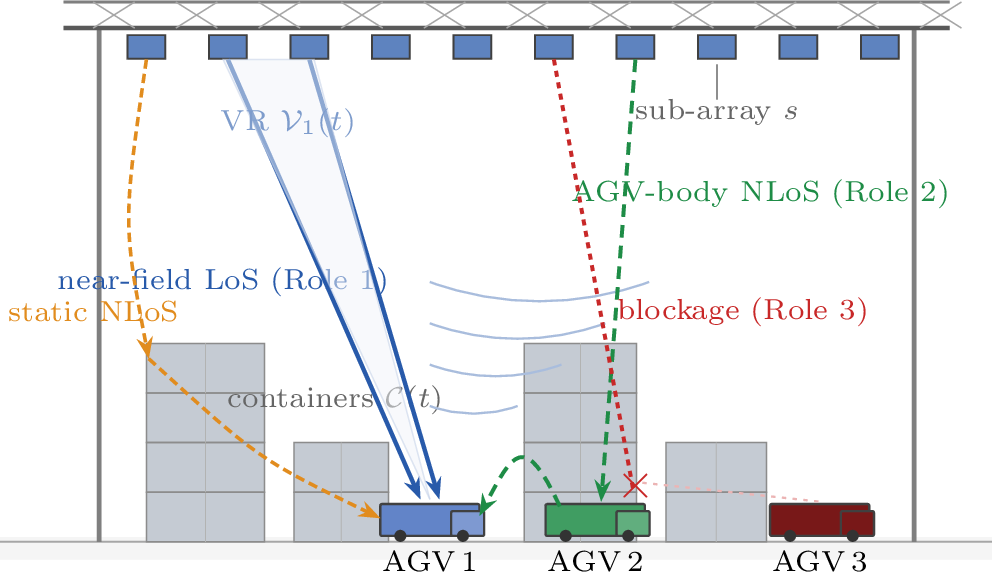
A modular XL-MIMO base station (BS) with \(M=S\,M_s\) antennas, partitioned into \(S\) sub-arrays of \(M_s\) elements each, serves \(K\) single-antenna AGVs on the downlink (Fig. 1). The BS is mounted at \(h_{base} =20m\), while AGVs travel at \(v=5-20km/h\). The container topology \(\mathcal{C}(t)\) is available from the terminal operating system and evolves much more slowly than AGV mobility. Unlike conventional XL-MIMO systems, each AGV simultaneously acts as a communication user, a metallic scatterer, and a blocker. For brevity, the slot index \(t\) is omitted from instantaneous channel quantities.

2.1 VR-Coupled Near-Field Channel↩︎

Let \(\delta_{k,s}\in\{0,1\}\) denote whether sub-array \(s\) is visible to AGV \(k\), with visibility region (VR) \(\mathcal{V}_k=\{s:\delta_{k,s}=1\}\). The aggregate channel is \[\boldsymbol{h}_k=\sum_{s=1}^{S}\delta_{k,s}\boldsymbol{h}_{k,s},\] where each visible sub-array follows the near-field Rician model \[\label{eq:rician} \boldsymbol{h}_{k,s}=\sqrt{\beta_{k,s}}\!\left(\sqrt{\tfrac{\kappa_{k,s}}{\kappa_{k,s}+1}}\,\boldsymbol{a}_s(\boldsymbol{p}_k)+\sqrt{\tfrac{1}{\kappa_{k,s}+1}}\,\boldsymbol{h}_{k,s}^{\text{NLoS}}\right)\!,\tag{1}\] with \(\beta_{k,s}\) the path gain, \(\kappa_{k,s}\) the Rician factor, and \(\boldsymbol{h}_{k,s}^{\text{NLoS}}\) defined in 3 . The near-field steering vector is \[\label{eq:steering} [\boldsymbol{a}_s(\boldsymbol{p}_k)]_m=\exp\!\Big(\!-j\tfrac{2\pi}{\lambda}\big(\|\boldsymbol{p}_k-\boldsymbol{u}_{s,m}\|-\|\boldsymbol{p}_k-\boldsymbol{u}_{s,0}\|\big)\Big),\tag{2}\] where \(\boldsymbol{p}_k\) is the AGV position, \(\boldsymbol{u}_{s,m}\) is the \(m\)-th antenna element of sub-array \(s\), and \(\boldsymbol{u}_{s,0}\) is its phase-reference center. Unlike conventional XL-MIMO models with static or user-independent VRs, \(\mathcal{V}_k\) depends jointly on the AGV position, the container topology, and neighboring AGVs, leading to coupled, time-varying visibility regions.

2.2 Triple-Role VR Coupling↩︎

The NLoS component comprises static container reflections and dynamic AGV-body scattering: \[\label{eq:nlos} \begin{align} \boldsymbol{h}_{k,s}^{\text{NLoS}}={}&\underbrace{\textstyle\sum_{\ell=1}^{L_{k,s}^{\text{C}}} g_{k,s,\ell}^{\text{C}}\,\boldsymbol{a}_s(\boldsymbol{q}_{k,s,\ell}^{\text{C}})}_{\text{container reflections}}\\[-2pt] &+\underbrace{\textstyle\sum_{j\neq k}\sum_{\ell=1}^{L_{k,s,j}^{\text{A}}} g_{k,s,j,\ell}^{\text{A}}\,\boldsymbol{a}_s(\boldsymbol{q}_{k,s,j,\ell}^{\text{A}})}_{\text{AGV-body scattering}}, \end{align}\tag{3}\] where container reflections depend on the topology \(\mathcal{C}(t)\), whereas AGV-induced paths depend on neighboring positions \(\{\boldsymbol{p}_j\}_{j\neq k}\) and disappear when \(L^{\text{A}}_{k,s,j}=0\).

Each AGV simultaneously acts as a communication user, a metallic scatterer, and a physical blocker. The blocking effect modifies the VR according to \[\label{eq:blocking} \delta_{k,s}=\delta_{k,s}^{\text{C}}\cdot\textstyle\prod_{j\neq k}\bigl(1-b_{k,s,j}\bigr),\tag{4}\] where \(\delta_{k,s}^{\text{C}}\) is the container-only VR indicator and \(b_{k,s,j}\in\{0,1\}\) indicates whether AGV \(j\) blocks the dominant path between sub-array \(s\) and AGV \(k\). Consequently, \[\label{eq:vr-coupled} \mathcal{V}_k=f\bigl(\boldsymbol{p}_k,\,\mathcal{C}(t),\,\{\boldsymbol{p}_j\}_{j\neq k}\bigr),\tag{5}\] so both \(\boldsymbol{h}_k\) and \(\mathcal{V}_k\) depend on the positions of all AGVs. Unlike conventional XL-MIMO models with independent user channels, the resulting inter-user coupling is dynamic yet predictable because AGV trajectories are coordinated by the terminal operating system.

2.3 Received Signal↩︎

With beamformer \(\boldsymbol{w}_k\in\mathbb{C}^M\) and unit-power symbol \(x_k\), AGV \(k\) receives \[\label{eq:rx} y_k=\boldsymbol{h}_k^H\boldsymbol{w}_k x_k+\sum_{j\neq k}\boldsymbol{h}_k^H\boldsymbol{w}_j x_j+n_k,\tag{6}\] where \(n_k\sim\mathcal{CN}(0,\sigma^2)\). Since \(\boldsymbol{h}_k\) is determined by the fleet-coupled VR model, both the desired signal and interference depend on the positions of neighboring AGVs. The resulting SINR and achievable rate are \[\label{eq:sinr} \gamma_k=\frac{|\boldsymbol{h}_k^H\boldsymbol{w}_k|^2}{\sum_{j\neq k}|\boldsymbol{h}_k^H\boldsymbol{w}_j|^2+\sigma^2},\qquad R_k=\log_2(1+\gamma_k),\tag{7}\] subject to the total transmit-power \(\sum_k\|\boldsymbol{w}_k\|^2\le P_{\text{tot}}\).

3 Two-Timescale VR-Aware Beamforming↩︎

We maximize the PF-weighted sum-rate over the slow-stage association \(\boldsymbol{A}\in\{0,1\}^{S\times K}\) (\(A_{s,k}=1\) if sub-array \(s\) may serve AGV \(k\)) and fast-stage beamformer \(\boldsymbol{W}\): \[\begin{align} \max_{\boldsymbol{A},\boldsymbol{W}}\;&\textstyle\sum_{k=1}^{K}\alpha_k R_k \label{eq:opt}\\ \text{s.t.}\;\; & A_{s,k}\le\delta_{k,s},\;\; \textstyle\sum_k A_{s,k}\le N_s^{\max},\;\; \textstyle\sum_s A_{s,k}\le L_k^{\max},\notag\\ & \mathrm{supp}(\boldsymbol{w}_k)\subseteq\{s:A_{s,k}=1\},\;\; \textstyle\sum_k\|\boldsymbol{w}_k\|^2\le P_{\text{tot}},\notag \end{align}\tag{8}\] where \(\alpha_k=1/\bar{R}_k\) is the PF weight (\(\bar{R}_k\) the historical mean rate), \(N_s^{\max}\) the per-sub-array user capacity, and \(L_k^{\max}\) the per-user sub-array budget. Problem 8 is mixed-integer and non-convex, and its variables live on different timescales: \(\boldsymbol{A}\) need change only with \(\mathcal{C}(t)\), whereas \(\boldsymbol{W}\) tracks fast fading and motion. We therefore decompose it.

3.1 Slow Stage: Association↩︎

Over a topology epoch we maximize a long-term surrogate. With \(\bar{\delta}_{k,s}=\mathbb{E}[\delta_{k,s}]\) and \(\bar{\beta}_{k,s}=\mathbb{E}[\beta_{k,s}]\) estimated by Monte-Carlo sampling of the fleet through the coupled map 5 , we solve the binary linear program \(\max_{\boldsymbol{A}}\sum_{s,k}U_{s,k}A_{s,k}\) subject to the first three constraints of 8 , with utility \[\label{eq:utility} U_{s,k}=\bar{\beta}_{k,s}-\gamma\!\textstyle\sum_{j\neq k}\bar{\delta}_{j,s}.\tag{9}\] The first term favors strong, reliably visible links; the contention penalty (\(\gamma>0\)) discourages overloading popular sub-arrays. Crucially, \(\bar{\delta}_{k,s}\) follows 4 over sampled positions, embedding AGV-blocking statistics; associating on the static \(\bar{\delta}^{\text{C}}_{k,s}\) instead systematically over-commits shadowed sub-arrays.

3.2 Fast Stage: Masked WMMSE↩︎

Given \(\boldsymbol{A}\) and instantaneous CSI, the effective active set is \(\mathcal{A}_k=\{s:A_{s,k}\delta_{k,s}=1\}\), i.e., the intersection of the association and instantaneous VR. The beamformer is restricted to \(\mathcal{I}_k=\bigcup_{s\in\mathcal{A}_k}\mathcal{M}_s\) through the diagonal mask \(\boldsymbol{D}_k\), where \([\boldsymbol{D}_k]_{mm}=1\) iff \(m\in\mathcal{I}_k\). Thus, once \(\boldsymbol{A}\) is fixed, the support is fixed and the beamforming subproblem becomes continuous. Applying WMMSE [10], the MMSE receiver, error, and PF-weighted MSE weight are \[\label{eq:wmmse-ue} u_k=\frac{\boldsymbol{h}_k^H\boldsymbol{w}_k}{\sum_j|\boldsymbol{h}_k^H\boldsymbol{w}_j|^2+\sigma^2},\;\; e_k=1-u_k^*\boldsymbol{h}_k^H\boldsymbol{w}_k,\;\; \omega_k=\frac{\alpha_k}{e_k},\tag{10}\] and the masked beamformer update is \[\label{eq:wmmse-v} \boldsymbol{w}_k=\boldsymbol{D}_k\Bigl(\textstyle\sum_j\omega_j|u_j|^2\,\boldsymbol{h}_j\boldsymbol{h}_j^H+\mu\boldsymbol{I}\Bigr)^{-1}\!\omega_k u_k\,\boldsymbol{h}_k,\tag{11}\] where \(\mu\ge0\) is obtained by bisection to satisfy the power constraint. Since \(\boldsymbol{D}_k\) suppresses inactive antennas, 11 operates only on the active set \(\mathcal{I}_k\).

After each slot, the PF weights are updated as \[\label{eq:pf-update} \bar{R}_k\leftarrow(1-\rho)\bar{R}_k+\rho R_k,\qquad \alpha_k=1/\bar{R}_k,\tag{12}\] so AGVs experiencing persistent blockage are assigned higher priority, improving long-term fairness.

3.3 Disjoint-VR Structure↩︎

The following proposition characterizes the structural objective of the slow-stage association. Let \(\mathcal{A}_k\) denote the effective active sub-array set of AGV \(k\), and let \(\mathcal{I}_k=\bigcup_{s\in\mathcal{A}_k}\mathcal{M}_s\) be its corresponding antenna support.

3.4 Complexity↩︎

The slow stage is dominated by Monte Carlo estimation of the coupled VR statistics, requiring \(\mathcal{O}(N_{\text{s}}KS(K+N_{\text{box}}))\) operations. Since it is executed only once per topology epoch, its amortized per-slot complexity is negligible.

For the fast stage, let \(M_k=|\mathcal{I}_k|\le L_k^{\max}M_s\) denote the number of active antennas for AGV \(k\). Each WMMSE iteration requires receiver/weight updates, construction of the active covariance sub-block, an \(\mathcal{O}(M_k^3)\) eigendecomposition, and power-control bisection, yielding \[\label{eq:complexity} \mathcal{O}\!\big(T\textstyle\sum_k(M_k^3+KM_k^2+T_\mu M_k)\big) =\mathcal{O}\!\big(TKM_{\text{a}}^3\big),\tag{13}\] where \(M_{\text{a}}=\max_k M_k\). In contrast, conventional full-array WMMSE scales as \(\mathcal{O}(TKM^3)\) with \(M=SM_s\). Since masking restricts each user to \(M_{\text{a}}\le L_k^{\max}M_s\ll M\), the per-user complexity is reduced by approximately \((S/L_k^{\max})^3\).

4 Simulation Results↩︎

We consider a \(400\times300\) m smart container terminal with eight storage lanes (stack height \(12\) m, lane width \(15\) m). Channels are generated using a geometry-based model: LoS is determined by 3D ray-box intersection, while NLoS consists of first- and second-order image-method reflections from PEC container walls. AGV bodies are modeled as \(3\times1.5\times1.5\) m PEC plates for both scattering and blocking. Unless otherwise stated, the system uses \(f_c=3.5\) GHz, \(M=512\) antennas (\(S=16\), \(M_s=32\)), \(P_{\text{tot}}=40\) dBm, \(N_s^{\max}=2\), \(L_k^{\max}=6\), \(\gamma=0.02\), \(T=5\) WMMSE iterations, and \(\rho=0.2\). The container topology is updated every \(30\) min with \(10\%\) of stacks reshuffled, and all results are averaged over five topology realizations and 100 time slots.

We compare the proposed scheme with three baselines: B1, a far-field stationary model with full-array WMMSE; B2, the proposed near-field model using only container-induced VRs (no AGV blocking or scattering); and B3, the full channel model with greedy sub-array association based on instantaneous \(\beta_{k,s}\). Performance is evaluated in terms of average sum-rate, outage probability, and the CDF of the per-user rate.

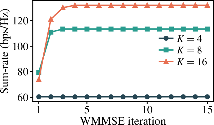
Convergence (Fig. 2). Despite restricting each user to its support \(\mathcal{I}_k\), the sum-rate increases monotonically and stabilizes within \(3\)–\(4\) iterations for all fleet sizes, confirming that the projection mask \(\boldsymbol{D}_k\) preserves the stationary-point convergence of standard WMMSE; we adopt \(T=5\) as a conservative default. Combined with the \((S/L_k^{\max})^3\) per-user cost reduction of 13 , the fast stage is both convergent and real-time.

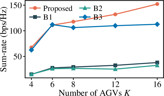
Sum-rate (Fig. 3). The proposed method beats VR-unaware B1/B2 by a wide margin for all \(K\), confirming that ignoring near-field geometry and the triple role wastes power on blocked or poorly focused sub-arrays. Against greedy B3 the two are essentially tied at low density (\(K=6\)), but the MILP association pulls ahead as \(K\) grows \(+10.9\%\) at \(K=8\), \(+20.1\%\) at \(K=12\), \(+35.0\%\) at \(K=16\). This widening gap is the signature of global load balancing under the tight capacity \(N_s^{\max}=2\): greedy overloads popular sub-arrays and starves contenders, whereas the MILP spreads load, so its advantage grows precisely as the fleet densifies.

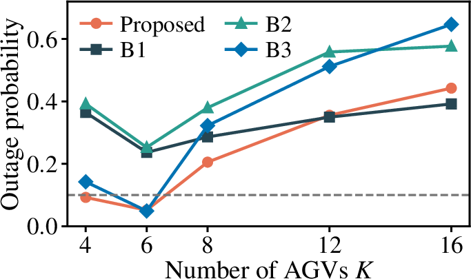
Outage (Fig. 4). All methods show a shallow minimum near \(K=6\); below it the occasional deep-canyon AGV inflates outage, above it contention drives it up. Among resource-constrained schemes the proposed method has the lowest outage: \(0.44\) at \(K=16\), vs.\(0.58\) (B2) and \(0.65\) (B3). Consistent with its rate distribution, it also serves the largest fraction of high-rate users and keeps the fewest in complete outage. The far-field B1 attains a slightly lower outage at high \(K\) (\(0.39\)) only by spreading power across all \(M\) antennas without the capacity limit \(N_s^{\max}\): this egalitarian allocation barely clears \(R_{\min}\) for most users while sacrificing over \(4\times\) the sum-rate (Fig. 3). Under the same resource budget the proposed design degrades the most gracefully while delivering far higher throughput. The absolute outage is high at large \(K\) because \(N_s^{\max}=2\) fundamentally limits how many AGVs can be served at once.

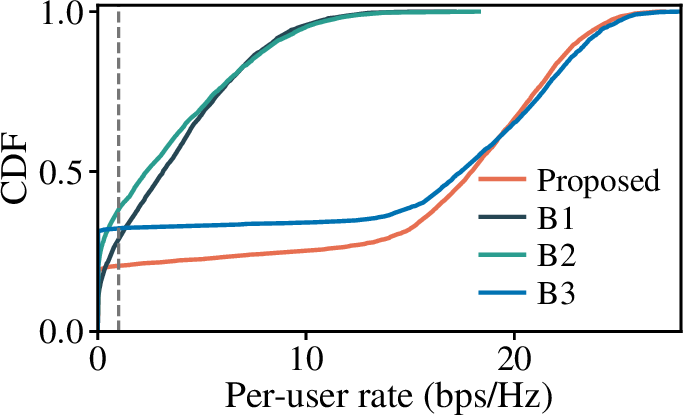
CDF (Fig. 5). The VR-unaware baselines B1 and B2 are concentrated at low rates, with median rates of approximately \(3\) and \(2.3\) bps/Hz, respectively, and nearly all users below \(15\) bps/Hz. This highlights the cost of ignoring near-field effects and the AGV triple role. In contrast, the proposed scheme shifts the distribution substantially to the right, achieving a median rate of \(17.9\) bps/Hz and a \(90\)th-percentile rate of \(22.9\) bps/Hz. It also reduces the outage probability (\(<\!1\) bps/Hz) to \(0.20\), compared with \(0.32\) for the greedy baseline B3. While some users remain in the moderate-rate region (\(1\)–\(15\) bps/Hz) due to the limited sub-array capacity (\(N_s^{\max}=2\)), the proposed scheme achieves the largest fraction of high-rate users and the lowest outage probability.

5 Conclusion↩︎

We identified the AGV’s triple role in smart-port XL-MIMO, where each AGV acts as a user, scatterer, and blocker, coupling user VRs and channels. We proposed a two-timescale masked WMMSE design that enforces VR support and reduces per-user complexity by \((S/L_k^{\max})^3\). We also established a disjoint-VR condition under which beamforming decouples and the PF rate bound is attained. Simulations show over \(3\times\) the sum-rate of VR-unaware baselines, with gains growing with fleet density. Predicting this coupling from AGV trajectories for proactive VR management is left for future work.

References↩︎