Backbone-Agnostic Perturbation-Induced Uncertainty Learning for End-to-End Real-World Image Dehazing
January 01, 1970
Abstract
Real-world paired image dehazing remains challenging because haze degradation is spatially non-uniform, illumination-dependent, and physically ambiguous even when haze-free references are available. Existing end-to-end restoration networks usually formulate dehazing as a deterministic mapping from a hazy observation to a clean target, leaving the uncertainty hidden in degraded features, haze priors, and cross-domain negative samples insufficiently explored. In this paper, we propose Backbone-Agnostic Perturbation-Induced Uncertainty Learning (BPUL), a plug-and-play uncertainty learning framework for end-to-end real-world image dehazing. BPUL first introduces a Learnable Perturbation-induced Uncertainty Modulator (LPUM) that estimates channel-wise and spatial-wise feature sensitivity through reparameterized stochastic perturbations. It then develops a Prior-informed Uncertainty-guided Reconstruction Module (PURM), which exploits transmission and atmospheric-light priors to reconstruct the hazy observation from the restored result and enforce degradation consistency. Furthermore, we propose a Dual-space Domain-diversified Distribution-aware Contrastive Loss (\(D^3\)CL) to regularize both clean restoration and hazy reconstruction spaces with real-world and synthetic negatives. Experiments on five real-world paired benchmarks show that BPUL consistently improves multiple representative backbones. Since only LPUM is retained during inference while PURM and \(D^3\)CL are used as training-time constraints, BPUL brings substantial restoration gains with only marginal additional inference overhead.
1 Introduction↩︎
Image dehazing aims to recover a visually faithful haze-free image from a hazy observation and remains a fundamental ill-posed low-level vision problem. The classical atmospheric scattering model describes a hazy image as \[I(x) = J(x)t(x) + A(1-t(x)),\] where \(I(x)\) and \(J(x)\) are the hazy observation and haze-free radiance, \(t(x)\) is the transmission map, and \(A\) is the global atmospheric light. Although this formulation motivates interpretable priors such as the dark channel prior [1], real haze rarely follows a deterministic pattern. Spatially varying density, illumination, depth ambiguity, camera response, and prior-estimation errors make real-world dehazing substantially more uncertain than standard supervised restoration.
Real-world paired datasets, including I-HAZE [2], O-HAZE [3], Dense-Haze [4], NH-HAZE [5], and LMHaze [6], enable quantitative evaluation with aligned hazy and haze-free pairs, yet also expose the ambiguity that paired supervision cannot remove. Dense haze suppresses texture and contrast, non-homogeneous haze varies spatially, and multi-intensity haze creates strong cross-scene shifts. Consequently, pixel-wise reconstruction alone can yield over-smoothed structures or color deviations despite visually plausible outputs.
Image restoration has progressed through stronger CNN and Transformer backbones [7]–[13], while dehazing methods increasingly exploit multi-scale feedback, color guidance, contrastive regularization, and uncertainty-aware processing [14]–[19]. Nevertheless, most end-to-end systems learn a deterministic mapping \(\hat{J}=f_{\theta}(I)\) dominated by restoration error. They do not explicitly identify degradation-sensitive channels and locations, test whether the restored image explains the observed haze under physical priors, or separate clean targets from real and synthetic degradation domains in feature space.
Uncertainty modeling provides a principled perspective, but estimating a full posterior for every feature is expensive and difficult to integrate into restoration backbones [20], [21]. We instead characterize haze uncertainty through feature sensitivity to learnable perturbations. Stable responses indicate reliable content, whereas sharp changes after perturbation and inverse alignment reveal degradation-sensitive information requiring adaptive modulation. Thus, uncertainty becomes a plug-and-play feature modulation signal rather than an isolated prediction head.
Motivated by this insight, we propose Backbone-Agnostic Perturbation-Induced Uncertainty Learning (BPUL) with three complementary components. The Learnable Perturbation-induced Uncertainty Modulator (LPUM) predicts channel-wise and spatial-wise perturbation distributions, uses reparameterized sampling and inverse alignment to derive uncertainty responses, and converts them into feature modulation weights. The Prior-informed Uncertainty-guided Reconstruction Module (PURM) reconstructs the hazy observation from the restored output with transmission and atmospheric-light priors, encouraging both clean appearance and degradation consistency. The Dual-space Domain-diversified Distribution-aware Contrastive Loss (\(\mathbf{D^3}\)CL) extends dehazing and restoration contrastive learning [15], [22]–[24] to clean restoration and hazy reconstruction spaces, using real and synthetic negatives together with stochastic perceptual features.
BPUL is backbone-agnostic and training-efficient: LPUM can be inserted into encoder-decoder restoration networks, whereas PURM and \(D^3\)CL act only as training-time constraints. Inference retains only lightweight LPUM components, without the reconstruction branch, negative samples, or perceptual contrastive computation. Experiments on five real-world paired benchmarks show consistent gains across representative backbones with marginal additional inference complexity.
Our contributions are summarized as follows:
We introduce BPUL, a backbone-agnostic perturbation-induced uncertainty learning framework for end-to-end real-world image dehazing, which explicitly models degradation-sensitive feature uncertainty through learnable stochastic perturbations.
We propose LPUM to estimate channel-wise and spatial-wise uncertainty responses from perturbation-induced feature discrepancies, enabling adaptive uncertainty-guided feature modulation without redesigning the underlying restoration backbone.
We design PURM to reconstruct the hazy observation from the restored result under transmission and atmospheric-light priors, thereby imposing a bidirectional physical-consistency constraint on real-world dehazing.
We develop \(D^3\)CL, a dual-space domain-diversified distribution-aware contrastive loss that regularizes clean restoration and hazy reconstruction with real-world and synthetic negatives in perturbation-aware perceptual feature space.
Extensive experiments and ablation studies on multiple real-world paired dehazing benchmarks demonstrate the effectiveness, generality, and interpretability of BPUL.
2 Related Work↩︎
2.1 Real-World Image Dehazing↩︎
Single-image dehazing recovers latent scene radiance from a hazy observation. Classical methods estimate transmission and atmospheric light under the atmospheric scattering model; the dark channel prior is a representative hand-crafted approach [1]. Deep methods replace manual estimation with trainable networks: DehazeNet predicts transmission [25], AOD-Net reformulates dehazing as an all-in-one mapping [26], and DCPDN jointly estimates physical variables and the clean image [27]. Later architectures improve representation with multi-scale feedback, attention, and Transformers, including GridDehazeNet [28], MSBDN [14], FFA-Net [29], and DehazeFormer [30]. Recent real-image methods further exploit codebook priors in RIDCP [31] and YCbCr-guided structural and color cues in SGDN [18].
Real paired datasets have shifted evaluation from synthetic haze toward realistic degradation. I-HAZE and O-HAZE provide indoor and outdoor pairs [2], [3]; Dense-Haze and NH-HAZE cover dense homogeneous and spatially non-homogeneous haze [4], [5]; and LMHaze introduces large-scale multi-intensity real haze [6]. These benchmarks reveal persistent ambiguity caused by variations in haze density, illumination, depth, and physical-prior estimation. Whereas most approaches learn deterministic restoration or prior-guided predictions, BPUL models degradation-sensitive feature uncertainty through learnable perturbation responses and uses it for feature modulation, physical-consistency training, and contrastive regularization.
2.2 Image Restoration↩︎
General image restoration has advanced through efficient CNNs, Transformers, and state-space models. Representative backbones include MIMOUNet [7], NAFNet [8], the efficient Transformers Restormer and Uformer [9], [10], prompt-conditioned all-in-one restoration [32], IRNeXt [33], OKNet [11], MaIR [34], HOGformer [12], and VIVNet [13]. Although these architectures provide strong deterministic restoration capacity, they do not explicitly model the uncertainty and physical ambiguity of real haze. BPUL complements such backbones by retaining only LPUM for uncertainty-aware inference, while PURM and \(D^3\)CL act as training-time regularizers.
3 Method↩︎
3.1 Overview↩︎
Given a real-world hazy image \(I\in\mathbb{R}^{3\times H\times W}\) and its paired haze-free image \(J\), our goal is to learn an end-to-end dehazing model that predicts a restored image \(\hat{J}=F_{\theta}(I)\) while explicitly modeling the degradation uncertainty hidden in real haze. Instead of designing a new restoration architecture, BPUL is a plug-and-play uncertainty learning framework that preserves the primary blocks and hierarchical topology of the selected backbone.
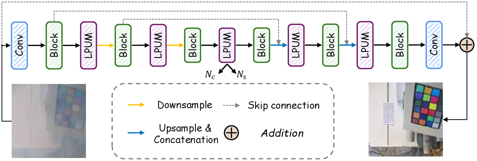
As illustrated in Figure 1, LPUM units modulate intermediate features at multiple resolutions without replacing the backbone blocks. The encoder progressively extracts degradation-aware representations, the decoder restores spatial detail through the original skip connections, and the final convolution predicts a residual that is added to the hazy input. This design allows the same uncertainty-learning principle to be embedded into CNN, Transformer, or hybrid restoration backbones with minimal architectural intervention.
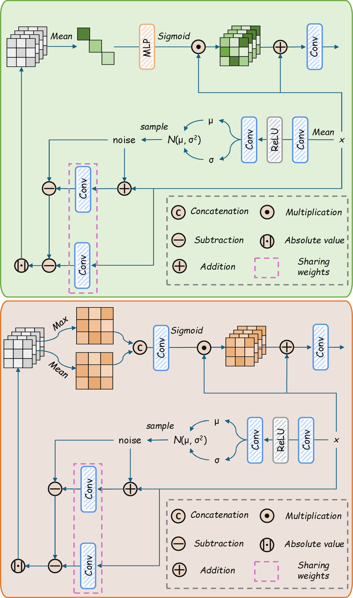
The complete training framework contains three complementary components, detailed in Figs. 2–4. LPUM produces uncertainty-modulated features and stochastic perturbation cues inside the restoration backbone. PURM then uses the restored result \(\hat{J}\), the hazy input \(I\), dark-channel-prior estimates of transmission and atmospheric light, and the perturbation cues shared from LPUM to reconstruct the original hazy image \(\hat{I}\). Finally, \(D^3\)CL regularizes both the clean restoration space and the hazy reconstruction space with real-world and synthetic negatives. During inference, only the LPUM-enhanced restoration path in Figure 1 is retained; PURM and \(D^3\)CL are discarded because they serve as training-time constraints.
3.2 Learnable Perturbation-induced Uncertainty Modulator↩︎
Most restoration backbones process a feature tensor deterministically, although real haze degradation affects different feature channels and spatial positions unevenly. LPUM is designed to reveal such degradation-sensitive responses by injecting learnable stochastic perturbations into intermediate features. Let \(X\in\mathbb{R}^{C\times H\times W}\) denote an intermediate feature map. LPUM first applies layer normalization and then estimates channel-wise and spatial-wise perturbation distributions.
For channel-wise uncertainty, LPUM uses global feature statistics to predict a mean and a logarithmic standard deviation: \[(\mu_c, \log \sigma_c) = f_c(\mathrm{GAP}(X)),\] where \(\mu_c,\sigma_c\in\mathbb{R}^{C\times 1\times 1}\). A channel perturbation is generated through reparameterized sampling: \[N_c = \mu_c + \sigma_c \odot \epsilon_c, \quad \epsilon_c\sim\mathcal{N}(0, I),\] which enables gradients to flow into the perturbation estimator. The sampled perturbation is broadcast along the spatial dimensions. LPUM then compares the original response and the inverse-aligned perturbed response: \[D_c = \left|\psi_c(X)-\left(\psi_c(X+N_c)-N_c\right)\right|,\] where \(\psi_c(\cdot)\) denotes a lightweight convolutional transformation. The discrepancy \(D_c\) measures how sensitive each channel is to stochastic haze-related perturbation. It is converted into a channel modulation vector by a sigmoid-gated mapping: \[W_c = \sigma\left(g_c(\mathrm{GAP}(D_c))\right).\]
For spatial-wise uncertainty, LPUM predicts a spatial perturbation distribution from local features: \[(\mu_s, \log \sigma_s) = f_s(X),\] where \(\mu_s,\sigma_s\in\mathbb{R}^{1\times H\times W}\). Similarly, the spatial perturbation is sampled as \[N_s = \mu_s + \sigma_s \odot \epsilon_s, \quad \epsilon_s\sim\mathcal{N}(0, I),\] then replicated across channels and injected into the input feature. The spatial response discrepancy is computed by \[D_s = \left|\psi_s(X)-\left(\psi_s(X+N_s)-N_s\right)\right|.\] To aggregate the discrepancy into a spatial modulation map, LPUM uses average and maximum statistics along the channel dimension: \[W_s = \sigma\left(g_s\left([\mathrm{Avg}_c(D_s), \mathrm{Max}_c(D_s)]\right)\right).\] The channel- and spatial-modulated features are fused with branch-wise residual compensation and a final residual connection: \[\begin{align} X_c &= X\odot W_c + X, \quad X_s = X\odot W_s + X, \\ \tilde{X} &= X + \eta_c(X_c) + \eta_s(X_s), \end{align}\] where \(\eta_c(\cdot)\) and \(\eta_s(\cdot)\) are lightweight convolutional projections. In this way, LPUM does not merely introduce random noise; it transforms perturbation-induced response discrepancies into uncertainty-aware feature modulation. The sampled bottleneck perturbations are also passed to PURM to couple forward dehazing and backward haze reconstruction.
3.3 Prior-informed Uncertainty-guided Reconstruction Module↩︎
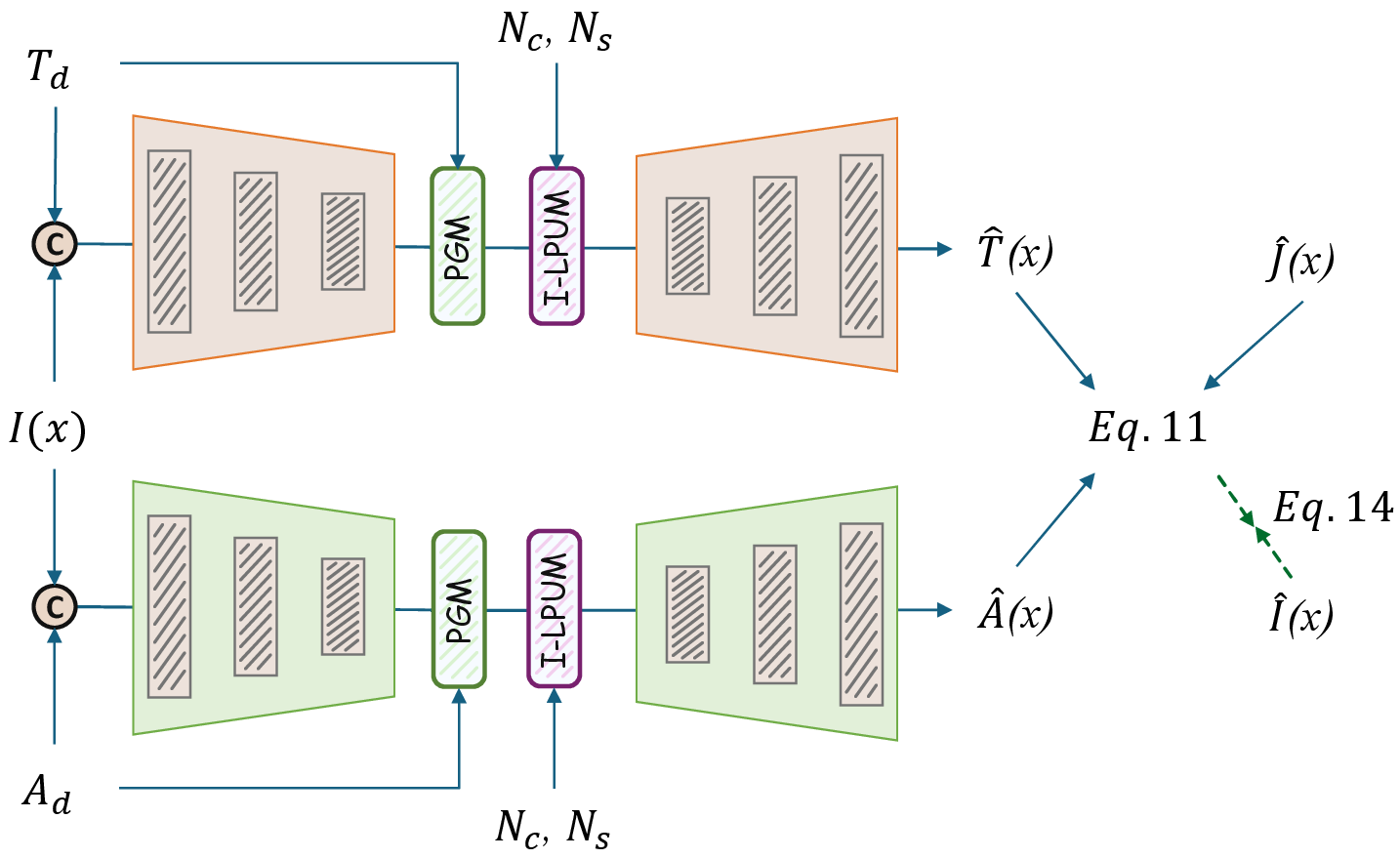
Pixel-wise supervision encourages \(\hat{J}\) to approach the haze-free target \(J\), but it does not guarantee that the prediction remains consistent with the observed haze formation process. To impose a bidirectional constraint, PURM reconstructs the hazy observation from the restored result. Based on the atmospheric scattering model, we formulate the reconstructed hazy image as \[\hat{I}(x)=\hat{T}(x)\hat{J}(x)+(1-\hat{T}(x))\hat{A}(x), \label{eq:purm95rec}\tag{1}\] where \(\hat{T}(x)\) and \(\hat{A}(x)\) are the transmission and atmospheric-light related maps predicted by PURM.
PURM contains two prior-informed reconstruction branches. The transmission branch takes the hazy image and a DCP-estimated transmission prior \(T_d\) as input, while the atmospheric-light branch takes the hazy image and a DCP-estimated atmospheric-light prior \(A_d\) as input. These priors are injected in two complementary ways. First, they are concatenated with the image input at multiple scales so that the reconstruction branch can exploit prior-aware local features. Second, they generate affine modulation parameters at the latent layer: \[Z_T' = Z_T \odot M_T(T_d) + B_T(T_d),\] \[Z_A' = Z_A \odot M_A(A_d) + B_A(A_d),\] where \(Z_T\) and \(Z_A\) denote latent representations in the transmission and atmospheric-light branches, and \(M(\cdot)\) and \(B(\cdot)\) represent prior-conditioned multiplicative and additive transformations. This affine guidance allows the physical priors to regulate the hidden reconstruction features instead of being used only as shallow concatenated inputs.
To further connect PURM with perturbation-induced uncertainty learning, the I-LPUM blocks in Figure 3 inherit \(N_c\) and \(N_s\) from the LPUM at the backbone bottleneck rather than estimating new perturbations. These cues modulate the latent features in both reconstruction branches. This design makes the reconstruction process uncertainty-guided: regions or channels that are more sensitive in the forward dehazing backbone also influence the backward haze reconstruction. The resulting reconstruction loss is defined as \[\mathcal{L}_{rec}=\rho(\hat{I}-I),\] where \(\rho(\cdot)\) denotes the Charbonnier penalty. PURM serves as a training-time reconstruction regularizer.
3.4 Dual-space Domain-diversified Distribution-aware Contrastive Loss↩︎
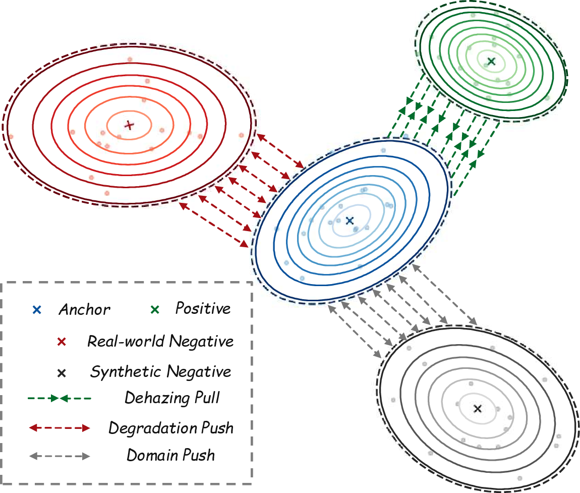
Conventional dehazing contrastive learning pulls the restored result toward the clean target and pushes it away from a negative hazy image in a deterministic perceptual feature space. However, real-world dehazing involves both clean restoration and haze reconstruction, and the negative domain may contain real-world haze and synthetic haze with different distributions. To address this issue, we propose \(D^3\)CL.
Let \(a\), \(p\), \(n\), and \(s\) denote an anchor, a positive sample, a real-world negative sample, and a synthetic negative sample, respectively. The real-world negative \(n\) is a non-corresponding hazy image sampled from another training pair, rather than the hazy input paired with the current positive sample. Since the paired ground truth already provides content-preserving supervision, such dataset-level real-haze negatives allow the contrastive objective to model the broader real-world degradation domain and avoid collapsing into a redundant paired reconstruction constraint. A frozen VGG-19 network extracts multi-level perceptual features \(\{\phi_l(\cdot)\}_{l=1}^{L}\). To approximate a distribution-aware feature representation without repeated network forwarding, we perturb each perceptual feature according to its activation magnitude: \[\tilde{\phi}_l(x)=\phi_l(x)+\epsilon_l\odot \sigma_l(x),\] \[\sigma_l(x)=\sqrt{\frac{r}{1-r}}\,|\phi_l(x)|, \quad \epsilon_l\sim\mathcal{N}(0,I),\] where \(r\) is a fixed perturbation ratio. This design provides an efficient approximation of stochastic perceptual feature distributions and avoids the high cost of multiple Monte Carlo VGG inferences.
The layer-wise distances are computed as \[d_l^{ap}=\left\|\tilde{\phi}_l(a)-\tilde{\phi}_l(p)\right\|_1,\] \[d_l^{an}=\left\|\tilde{\phi}_l(a)-\tilde{\phi}_l(n)\right\|_1, \quad d_l^{as}=\left\|\tilde{\phi}_l(a)-\tilde{\phi}_l(s)\right\|_1.\] Then \(D^3\)CL is formulated as \[\mathcal{L}_{D^3\mathrm{CL}}(a,p,n,s) =\sum_{l=1}^{L}\lambda_l\frac{1}{2} \left( \frac{d_l^{ap}}{d_l^{an}+\varepsilon} + \frac{d_l^{ap}}{d_l^{as}+\varepsilon} \right), \label{eq:d3cl}\tag{2}\] where \(\lambda_l\) balances different VGG layers and \(\varepsilon\) avoids numerical instability. In our implementation, we use five VGG feature levels with \(\{\lambda_l\}_{l=1}^{5}=\{1/32,1/16,1/8,1/4,1\}\) and set \(r=0.2\). The two denominator terms correspond to the real-world degradation push and the synthetic-domain push, respectively.
We apply \(D^3\)CL in two spaces. In the clean restoration space, the dehazed output \(\hat{J}\) is treated as the anchor, the clean image \(J\) is the positive sample, and real-world and synthetic negative samples are used to enlarge the degradation margin: \[\mathcal{L}_{clean}^{D^3\mathrm{CL}}=\mathcal{L}_{D^3\mathrm{CL}}(\hat{J},J,N_r,N_s).\] In the hazy reconstruction space, the reconstructed hazy image \(\hat{I}\) is treated as the anchor and the original hazy image \(I\) is the positive sample: \[\mathcal{L}_{hazy}^{D^3\mathrm{CL}}=\mathcal{L}_{D^3\mathrm{CL}}(\hat{I},I,N_r^h,N_s^h).\] This dual-space formulation simultaneously constrains the forward dehazing output and the backward haze reconstruction, making the contrastive regularization consistent with the bidirectional design of BPUL.
3.5 Training Objective and Inference↩︎
The overall training objective combines restoration supervision, haze reconstruction supervision, and dual-space contrastive regularization: \[\begin{align} \mathcal{L} = &\;\rho(\hat{J}-J) + \rho(\hat{I}-I) \\ &+ \frac{1}{2}\mathcal{L}_{clean}^{D^3\mathrm{CL}} + \frac{1}{2}\mathcal{L}_{hazy}^{D^3\mathrm{CL}}. \end{align} \label{eq:total95loss}\tag{3}\] The first term trains the backbone to restore the haze-free image. The second term enforces physical consistency by reconstructing the hazy observation. The last two terms regularize the feature distributions in both clean and hazy spaces.
At inference time, only the restoration backbone equipped with LPUM is used: \[\hat{J}=F_{\theta}^{\mathrm{LPUM}}(I).\] PURM is removed during inference. Therefore, the additional inference cost of BPUL comes only from the lightweight LPUM operations inserted into the backbone, while the stronger physical and contrastive constraints benefit training without slowing down deployment.
4 Experiments↩︎
4.1 Experimental Setup↩︎
Datasets. We evaluate BPUL on five real-world paired image dehazing benchmarks with distinct degradation characteristics: Dense-Haze [4], I-HAZE [2], O-HAZE [3], NH-HAZE [5], and LMHaze [6]. Dense-Haze contains dense homogeneous haze, I-HAZE and O-HAZE focus on indoor and outdoor real haze, respectively, NH-HAZE introduces spatially non-homogeneous haze, and LMHaze covers large-scale scenes with multiple haze intensities. The main training set aggregates 4,065 paired images: 40 from Dense-Haze, 25 from I-HAZE, 35 from O-HAZE, 40 from NH-HAZE, and 3,925 from LMHaze. Evaluation uses 15, 5, 10, 15, and 1,115 test pairs from these datasets, respectively. We report peak signal-to-noise ratio (PSNR) and structural similarity index (SSIM); higher values indicate better restoration quality.
Compared methods. We compare against representative image restoration and dehazing networks, including MIMOUNet [7], NAFNet [8], IRNeXt [33], OKNet [11], SGDN [18], MaIR [34], UHDPromer [35], \(\mathrm{C}^2\)SSM [36], HOGformer-S [12], and VIVNet [13]. To assess backbone generality, BPUL is separately integrated into MIMOUNet, IRNeXt, HOGformer-S, and VIVNet without redesigning their primary restoration blocks. For each baseline/BPUL pair, the data processing, optimization, and evaluation protocols are kept identical.
4.2 Comparison with State-of-the-Art Methods↩︎
| Method | Venue | GFLOPs | Params. | Dense-Haze | I-HAZE | O-HAZE | NH-HAZE | LMHaze | Average |
|---|---|---|---|---|---|---|---|---|---|
| MIMOUNet | ICCV’21 | 16.81 | 6.81 | 15.49/0.576 | 18.80/0.813 | 21.50/0.861 | 16.69/0.674 | 18.46/0.752 | 18.19/0.735 |
| NAFNet | ECCV’22 | 4.03 | 17.11 | 14.47/0.471 | 16.81/0.723 | 20.47/0.836 | 15.61/0.634 | 17.68/0.703 | 17.01/0.673 |
| IRNeXt | ICML’23 | 10.55 | 5.46 | 16.51/0.599 | 17.33/0.786 | 23.58/0.875 | 16.43/0.647 | 18.09/0.747 | 18.39/0.731 |
| OKNet | AAAI’24 | 9.93 | 4.72 | 13.91/0.534 | 17.07/0.758 | 21.67/0.852 | 15.18/0.595 | 17.62/0.716 | 17.09/0.691 |
| SGDN | AAAI’25 | 13.44 | 11.09 | 13.50/0.460 | 15.28/0.727 | 16.45/0.744 | 14.30/0.523 | 16.48/0.614 | 15.20/0.614 |
| MaIR | CVPR’25 | 3.18 | 3.40 | 14.90/0.506 | 16.60/0.719 | 19.96/0.842 | 14.99/0.625 | 18.22/0.731 | 16.93/0.685 |
| UHDPromer | IJCV’26 | 0.512 | 0.742 | 13.42/0.484 | 14.54/0.655 | 15.93/0.765 | 13.52/0.594 | 16.83/0.655 | 14.85/0.630 |
| \(\mathrm{C}^2\)SSM | CVPR’26 | 1.65 | 2.84 | 13.39/0.420 | 16.34/0.720 | 17.78/0.771 | 13.36/0.542 | 16.91/0.645 | 15.56/0.619 |
| HOGformer-S | AAAI’26 | 6.05 | 4.31 | 15.74/0.562 | 18.46/0.759 | 20.94/0.852 | 16.01/0.666 | 17.91/0.730 | 17.81/0.714 |
| VIVNet | TPAMI’26 | 16.17 | 7.42 | 15.19/0.569 | 18.00/0.784 | 22.49/0.861 | 17.09/0.697 | 18.46/0.760 | 18.24/0.734 |
| MIMOUNet+BPUL | Ours | 17.39 | 6.95 | 16.05/0.592 | 20.81/0.848 | 23.54/0.887 | 17.21/0.709 | 19.01/0.796 | 19.32/0.767 |
| IRNeXt+BPUL | Ours | 11.12 | 5.60 | 16.63/0.602 | 19.93/0.818 | 24.58/0.882 | 17.18/0.679 | 18.46/0.783 | 19.36/0.753 |
| HOGformer-S+BPUL | Ours | 6.56 | 4.40 | 16.81/0.619 | 19.96/0.844 | 23.49/0.892 | 17.37/0.728 | 18.88/0.792 | 19.30/0.775 |
| VIVNet+BPUL | Ours | 17.44 | 7.74 | 16.65/0.600 | 18.94/0.828 | 24.15/0.895 | 17.84/0.739 | 19.12/0.799 | 19.34/0.772 |
![Figure 5: Qualitative comparison. (a) Input; (b) MIMOUNet [7]; (c) MIMOUNet+BPUL; (d) IRNeXt [33]; (e) IRNeXt+BPUL; (f) HOGformer-S [12]; (g) HOGformer-S+BPUL; (h) VIVNet [13]; (i) VIVNet+BPUL; and (j) ground truth (GT). Following the error-map visualization of[37], each panel stacks the RGB result (top) and its absolute error relative to ground truth (bottom), because subtle restoration differences can be difficult to distinguish by visual inspection alone. Darker error-map colors indicate larger errors.](/article/2607.11623/_pdflatex/bjzfxlsn.png "fig:")
Table 1 reports the quantitative comparison. BPUL consistently improves all four backbones on every benchmark, despite their substantially different convolutional, Transformer, and hybrid restoration designs. On average, BPUL improves MIMOUNet by \(1.13\) dB/\(0.031\) SSIM, IRNeXt by \(0.96\) dB/\(0.021\) SSIM, HOGformer-S by \(1.48\) dB/\(0.061\) SSIM, and VIVNet by \(1.09\) dB/\(0.038\) SSIM. These consistent gains support the backbone-agnostic nature of perturbation-induced uncertainty learning rather than an architecture-specific enhancement.
The four BPUL-enhanced networks also surpass all standalone competitors in average PSNR and SSIM. Their advantages remain evident across degradation types: HOGformer-S+BPUL performs best on Dense-Haze, MIMOUNet+BPUL achieves the strongest I-HAZE result, IRNeXt+BPUL obtains the highest O-HAZE PSNR, and VIVNet+BPUL performs best on NH-HAZE and LMHaze. This cross-dataset behavior indicates that BPUL improves not only the mean restoration accuracy but also robustness to indoor/outdoor scenes, homogeneous/non-homogeneous haze, and varying haze intensity.
4.3 Ablation Studies↩︎
| Configuration | PSNR | SSIM |
|---|---|---|
| Baseline | 17.14 | 0.698 |
| w/o channel-wise branch | 17.40 | 0.716 |
| w/o spatial-wise branch | 17.43 | 0.719 |
| w/o learnable perturbation | 17.32 | 0.711 |
| Direct discrepancy weighting | 17.32 | 0.713 |
| Full LPUM | 17.56 | 0.725 |
| w/o \(T_d\) and \(A_d\) input | 17.36 | 0.703 |
| w/o \(T_d\) input | 17.39 | 0.718 |
| w/o \(A_d\) input | 17.38 | 0.715 |
| w/o latent affine guidance | 17.53 | 0.725 |
| w/o uncertainty modulation | 17.68 | 0.729 |
| Independent perturbations | 17.85 | 0.741 |
| Full PURM (shared \(N_c,N_s\)) | 18.03 | 0.753 |
Effect of LPUM. The upper part of Table 2 validates the roles of LPUM. Removing either the channel-wise or spatial-wise branch degrades performance, indicating that real-haze uncertainty is expressed jointly across feature channels and spatial locations. Disabling learnable perturbation generation reduces PSNR from \(17.56\) to \(17.32\) dB, demonstrating that the learned perturbation distributions are important for exposing degradation-sensitive responses. Direct discrepancy weighting is also inferior to the complete design, confirming that raw perturbation responses should be adaptively mapped before feature modulation. Overall, LPUM improves the baseline by \(0.42\) dB and \(0.027\) SSIM.
Effect of PURM. The lower part of Table 2 follows the progressive construction of PURM. Removing both \(T_d\) and \(A_d\) input injection causes the largest degradation among the prior-input variants, while removing either prior individually also lowers performance, showing that transmission and atmospheric-light cues are complementary. Latent affine guidance further improves the reconstruction branch beyond shallow input concatenation. Removing uncertainty modulation reduces the result to \(17.68/0.729\), verifying that physical priors alone do not fully exploit degradation-sensitive information. Finally, independently estimating perturbations in PURM reduces performance from \(18.03/0.753\) to \(17.85/0.741\), directly supporting cross-module uncertainty sharing between forward dehazing and backward haze reconstruction.
| Configuration | PSNR | SSIM |
|---|---|---|
| \(\mathcal{L}_{char}\) only | 17.14 | 0.698 |
| \(+\) conventional CRL | 17.73 | 0.739 |
| \(+\) non-corresp. real negative | 17.79 | 0.742 |
| \(+\) synthetic negative domain | 17.84 | 0.754 |
| \(+\) stochastic VGG features | 17.93 | 0.757 |
| Symmetric KL distance | 17.63 | 0.733 |
| \(W_2\) distance | 17.64 | 0.736 |
| Full \(D^3\)CL (clean+hazy) | 18.23 | 0.767 |
Effect of \(D^3\)CL. Table 3 presents the design evolution from the \(\mathcal{L}_{char}\) only to the complete \(D^3\)CL. Conventional contrastive regularization already improves the baseline, while replacing the paired input negative with a non-corresponding real hazy image provides an additional gain by broadening the modeled real-haze domain. Introducing a synthetic negative further improves SSIM from \(0.742\) to \(0.754\), confirming that real and synthetic haze form complementary negative domains. Stochastic VGG features increase the result to \(17.93/0.757\), whereas symmetric KL and Wasserstein-2 distances are less effective than sampled \(\ell_1\) distance under the same clean-space setting. Extending contrastive regularization to the reconstructed-hazy space finally yields \(18.23/0.767\), improving the baseline by \(1.09\) dB and \(0.069\) SSIM.
4.4 Qualitative and Mechanism Analysis↩︎
Figure 5 visually corroborates the quantitative improvements under outdoor and multi-intensity real haze. Since small restoration differences are often difficult to judge from RGB outputs alone, we additionally report absolute error maps relative to ground truth, following the visualization strategy in Windowing Decomposition Convolutional Neural Network for Image Enhancement [37]. Across both scenes, BPUL reduces residual haze and color deviation while preserving fine structures; the corresponding maps contain fewer dark high-error regions. The consistent gains across diverse backbones support BPUL’s architecture-agnostic design.
Figure 6: 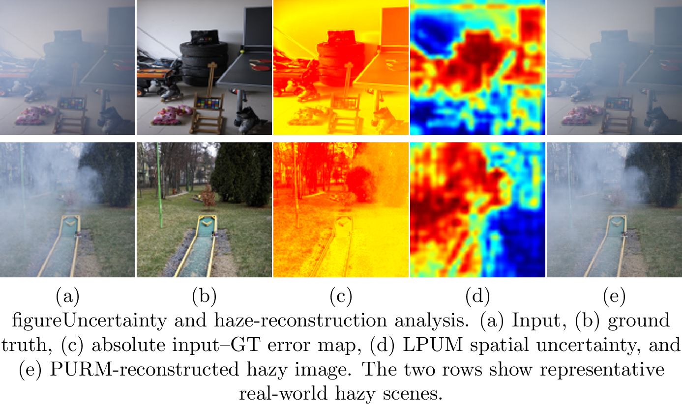 .
.
As shown in Figure 6, the input–GT error map directly visualizes the spatial haze degradation, while the learned LPUM response emphasizes degradation-sensitive regions in feature space. The two maps are related but are not expected to coincide exactly: the former measures pixel-level appearance difference, whereas the latter reflects sensitivity to learned perturbations. PURM further reconstructs the dominant haze appearance and spatial distribution from the dehazed result, supporting the complementary roles of forward uncertainty modulation and reverse degradation consistency.
5 Conclusion↩︎
We presented BPUL, a backbone-agnostic perturbation-induced uncertainty learning framework for end-to-end real-world image dehazing. BPUL uses LPUM to transform learnable perturbation responses into channel-wise and spatial-wise feature modulation, PURM to impose prior-informed reverse haze reconstruction, and \(D^3\)CL to regularize clean and hazy feature distributions with diversified negative domains. Experiments on five real-world paired benchmarks demonstrate consistent improvements across four representative restoration backbones, while the training-only PURM and contrastive branches are removed at inference. These results show that explicitly learning degradation-sensitive uncertainty and enforcing bidirectional degradation consistency provide a general and efficient way to strengthen real-world dehazing networks.