Abstract
Model editing keeps large language models (LLMs) up to date without retraining, but temporal facts expose a limitation of the prevailing locate-and-edit paradigm: an update is not always a replacement. When a fact changes, the new answer should become current while the old answer may remain correct in historical time contexts. Building on this insight, we use causal tracing to show that LLMs already support this distinction via a two-stage internal computation: early MLP layers retrieve a time-agnostic subject representation, and later layers modulate it with temporal context to yield the time-correct answer. Motivated by this finding, we introduce PRISM Edit, which optimizes a single polysemous representation across temporal contexts and leverages the model’s inherent modulation pathway to route it to temporally correct predictions—without any architectural modification. We evaluate on TimeConflict, a new temporal editing benchmark we introduce, and on temporally augmented CounterFact. PRISM Edit improves over the best baseline by +23.3 Temporal Consistency (TC) and +33.7 Current Relative-time Score (CRS) on average while being more than \(2\times\) faster. Code and data are publicly available in an anonymized repository at https://anonymous.4open.science/r/PRISM-Edit-ABE2.
1 Introduction↩︎
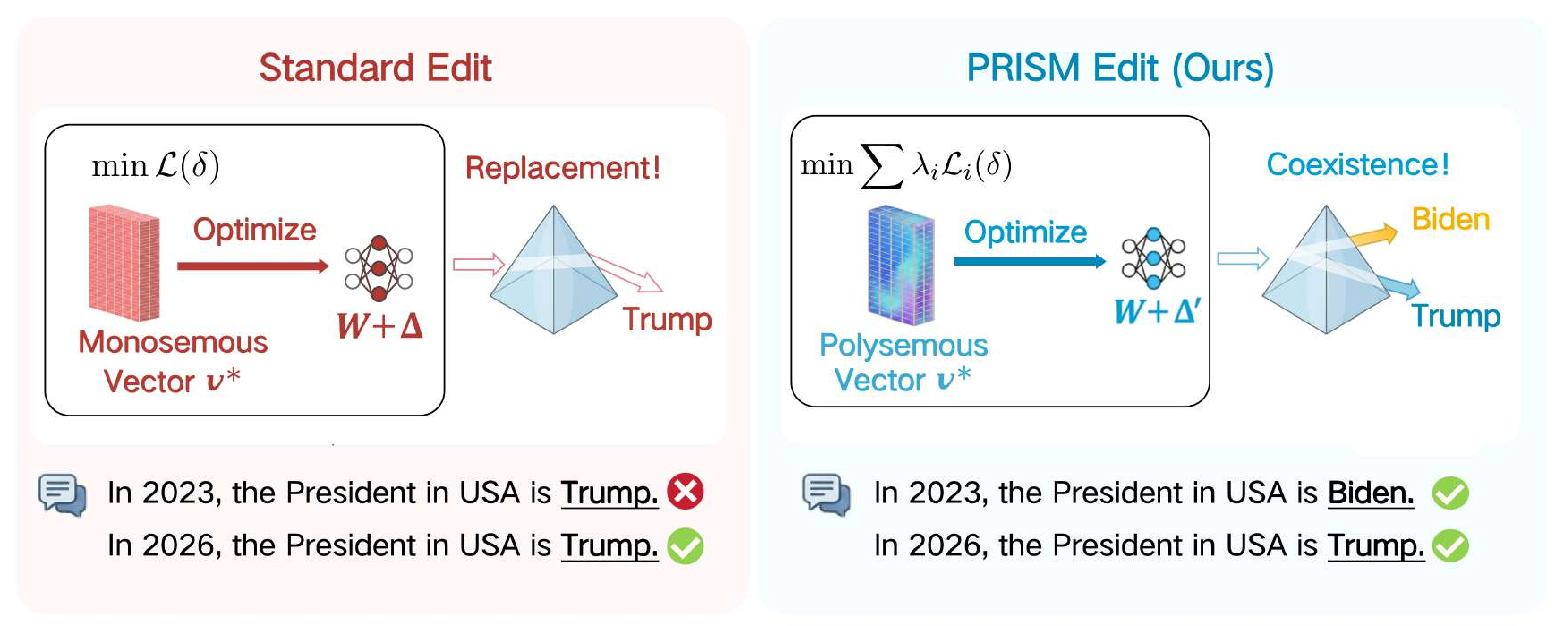
Large language models store extensive factual knowledge, yet the world they describe keeps changing. Knowledge editing allows models to continuously acquire new knowledge without full retraining, typically by modifying a small set of parameters associated with a target memory [1]–[6]. However, existing methods implicitly assume that every edit is a wholesale replacement of the old fact. This assumption breaks down for temporal facts, where the old answer does not become wrong—it merely ceases to be current. For example, when the U.S. presidency transfers from Biden to Trump in January 2025, the new fact should become current, yet “Who was the U.S.president in 2023?” must still return Biden. A temporal editor must therefore perform a harder operation: incorporate the new answer while preserving the historical conditions under which the old answer is still true.
The difficulty lies in the locate-and-edit paradigm itself: it locates a factual association \((s, r, o)\) and overwrites it with a new target \(o'\). This works for single-valued facts, but it mismatches temporal knowledge, where the same \((s, r)\) pair can map to different objects under different time contexts. As a result, standard editors often collapse time-conditioned behavior into a single edited answer, degrading historical recall after temporal edits [7]–[9] (Figure 1). Existing temporal-editing strategies attempt to patch this gap by storing separate parameters per time period [9] or splitting updates into multiple independent edits [7]. Yet these approaches leave a key question unanswered: if the unedited model can already answer time-conditioned prompts, why should editing ignore the model’s own temporal computation?
We take a fundamentally different approach. Rather than imposing external temporal structure, we first ask how the model internally resolves temporal ambiguity, and then design an editing method that works with—not against—this mechanism. Through causal tracing on \((s, r, o, t)\) tuples (§3), we discover that subject retrieval at early MLP layers is time-agnostic, while temporal disambiguation emerges via later-layer modulation of the same subject signal. This finding motivates PRISM Edit (Polysemous Representation via Intrinsic Signal Modulation): we write a single polysemous \(v^*\) into the model and let the model’s own downstream temporal modulation route the representation to time-correct answers—requiring no architectural changes, no auxiliary modules, and no per-period storage.
Our main contributions are as follows:
We reveal through causal tracing on \((s,r,o,t)\) tuples that large language models process temporal knowledge via a two-stage mechanism: time-agnostic subject retrieval at early MLP layers, followed by later-layer temporal modulation of the same subject signal (§3).
We formalize temporal polysemy and propose PRISM Edit, which reconceptualizes temporal editing from writing separate per-period facts to writing a single polysemous \(v^*\) that the model’s own modulation disambiguates—requiring no architectural changes or auxiliary modules (§4).
We introduce TimeConflict, a temporal editing benchmark spanning 24 relations and 22,708 records, and show that PRISM Edit achieves state-of-the-art performance across TimeConflict and temporally augmented CounterFact, improving over the best baseline by \(+23.3\) TC and \(+33.7\) CRS on average while being more than \(2\times\) faster on temporal editing tasks (§5).
2 Related Work↩︎
2.1 Locate-then-Edit Knowledge Editing↩︎
Knowledge editing enables efficient updates of specific facts in LLMs without full retraining [5]. Among various approaches, the locate-then-edit paradigm has proven particularly effective by first identifying where knowledge is stored and then directly modifying the corresponding parameters. ROME [3] applies causal tracing to locate factual associations in mid-layer MLP modules and performs rank-one weight updates. MEMIT [4] extends this to batch editing by distributing updates across multiple critical layers. AlphaEdit [6] further projects updates into the null space of preserved knowledge to minimize interference with unrelated facts. Other paradigms such as external memory approaches [2], [10] and dual-memory architectures [11] avoid direct parameter modification but introduce additional inference overhead. However, all these methods treat knowledge as temporally static, ignoring that historical facts remain valid within their original time scope.
2.2 Temporal Knowledge Editing↩︎
Real-world knowledge evolves over time, yet most editing methods treat facts as temporally static, simply overwriting old facts with new ones. Early work probes this temporal dimension on the language modeling side: [12] introduce TempLAMA and show that LMs encode temporally scoped facts but quickly become stale, motivating time-aware updates. [7] first formalized temporal knowledge editing (TKE), arguing that historical facts remain valid within their original time scope and proposing the AToKe benchmark. Subsequent work has explored this direction from various angles: Temple-MQA [8] constructs temporal knowledge graphs for time-aware multi-hop reasoning, and SPIKE [9] introduces sparse parameter injection anchored to temporal markers for multi-granularity temporal editing. Our method, PRISM Edit, takes a fundamentally different approach: we jointly optimize a single time-agnostic \(v^*\), allowing the model to naturally produce different answers based on temporal context.
3 Tracing Temporal Knowledge in LLMs↩︎

In this section, we investigate how large language models internally process temporal knowledge through causal tracing and representational similarity analysis.
3.1 Methods↩︎
Understanding how temporal context influences factual retrieval requires tracing information flow across the model’s internal layers. To this end, we adopt causal tracing [3], a probing technique that measures the causal contribution of individual hidden states to a model’s prediction. The procedure involves three runs: (1) a clean run that records all hidden states under uncorrupted inputs, (2) a corrupted run that adds Gaussian noise to a selected token group at the embedding layer, yielding a degraded prediction, and (3) a restore run that restores a single (token, layer, component) activation to its clean-run value, while leaving all other activations at their corrupted values. From this, the indirect effect (IE) is defined as \(P_{\text{restore}}(\text{correct answer}) - P_{\text{corrupted}}(\text{correct answer})\), measuring how much restoring a single activation recovers the model’s prediction, thereby identifying which activations are causally responsible for factual recall.
For standard \((s, r, o)\) triplets, causal tracing has localized factual recall to the early MLP layers [13] at the subject’s last token, where the indirect effect peaks. Temporal knowledge, however, follows an extended \((s,r,o,t)\) structure, where producing the correct answer demands not only recognizing the subject but also anchoring in time. This raises a key question: how do subject and temporal signals jointly determine the model’s prediction?
To answer this, we extend causal tracing to disentangle subject and temporal contributions. Rather than corrupting subject tokens as a whole, we corrupt subject tokens and time tokens separately, obtaining individual IE maps for each information pathway. Concretely, we compute the average IE on LLaMA-3-8B-Instruct [14] over 500 temporal knowledge pairs that the model answers correctly, varying the choice of mediator over all (token, layer, component) triplets with component \(\in\) . See Appendix 8 for more details.
Additionally, we perform a representational similarity analysis: for the same subject under new-time vs.old-time prompts, we compute layer-wise cosine similarity of hidden states at key token positions, revealing how temporal information progressively affects representations across layers.
3.2 Findings↩︎
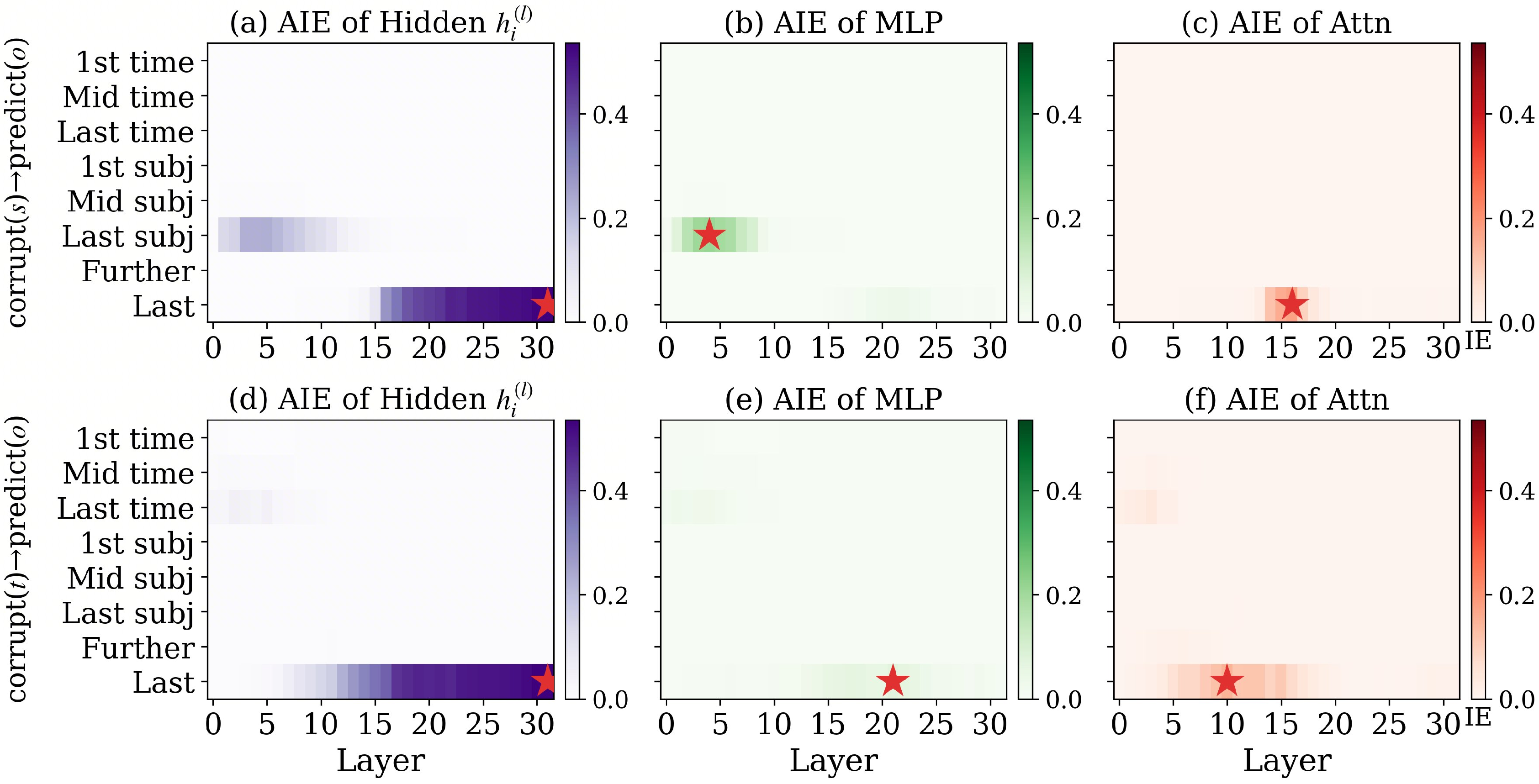
The resulting AIE maps (Figure 2) show a striking asymmetry: subject effects concentrate at the early MLP layers (L4–8) of the subject-last token, while temporal effects are more distributed across positions and components. Combined with the representational similarity analysis (Figure 3), these maps reveal three key findings on the model’s temporal processing mechanism:
3.2.0.1 Finding 1: Subject retrieval is time-agnostic.
Consistent with prior work on factual recall [3], [4], [15], [16], our causal tracing confirms the early MLP layers (L4–8) at the last subject token as the core knowledge-storage site, with the largest indirect effect peaking at L4 MLP (IE=0.549; Figure 2b). What is new, however, is that this abstract knowledge retrieval is largely time-agnostic, supported by two converging pieces of evidence: (i) the last subject representation forms a plateau (\(\cos \geq 0.97\)) across the critical MLP layers (L4–8) (Figure 3, orange), showing that the subject representation is nearly invariant to different temporal context; (ii) when time tokens are corrupted (Figure 2e), the IE at the last subject early MLP layers remains negligible, indicating that temporal information rarely enters the subject pathway.
3.2.0.2 Finding 2: Temporal context arrives early but acts late.
To the last token, temporal information actually arrives earlier than subject information: attention layers around L10–15 carry temporal context to the prediction position (IE=0.356 at L10, Figure 2f), several layers before the subject signal is transported to the last token via L16 attention (Figure 2c). Yet its effect on the output does not manifest immediately. Figure 3 (blue) shows that the two temporal prompts first converge in the middle layers (cosine rising to \(\approx 0.82\)). This convergence is driven by the subject signal: arriving at the last token via L16 attention, the (shared) subject representation momentarily dominates the hidden state, masking the temporal differences between the two prompts. This attention-mediated temporal pathway is also supported by the recently identified Temporal Heads [17]. Only in the upper layers do the two prompts diverge (cosine dropping to \(\approx 0.70\)), reflecting temporal modulation that acts only after the subject signal is in place. Together with Finding 1, this reveals a two-stage mechanism: the subject signal arrives and dominates the last-token representation (convergence); the temporal signal, which arrived earlier, yet modulates this subject-grounded signal in the upper layers (divergence).
3.2.0.3 Finding 3: The editing site cannot discriminate time.
Findings 1 and 2 together expose a fundamental obstacle to locate-and-edit methods (see Section 2.1) on temporal facts. Since these methods edit the MLP at the subject-last token, where \(k\) is the input that conditions the write, any linear update \(\Delta W\) at this layer satisfies \[\|\Delta W\, k_{\text{new}} - \Delta W\, k_{\text{old}}\| \;\leq\; \|\Delta W\| \cdot \underbrace{\|k_{\text{new}} - k_{\text{old}}\|}_{\approx\, 0}. \label{eq:edit-collapse}\tag{1}\] where \(k_{\text{new}}\) and \(k_{\text{old}}\) denote the MLP input at the subject-last token under the new-time and old-time prompts, respectively. In other words, the two temporal prompts cannot be used as distinct retrieval conditions, so a single edit cannot deliver different values \(v_{\text{new}}\) and \(v_{\text{old}}\) for them. This is a geometric limit of the representation space, not a failure of optimization—no choice of optimizer or objective can recover what the keys cannot distinguish. And it is exactly why methods that try to edit different answers for different times, such as METO [7], fail at this layer.
3.2.0.4 Design implication for editing.
Taken together, the three key findings describe a coherent intrinsic mechanism: one time-agnostic subject signal plus later temporal modulation yields different answers. This naturally suggests the right design principle: instead of forcing the edit layer to separate time—something it cannot do, as Equation 1 shows—we should let the model’s own temporal modulation pathway handle the disambiguation. The next section formalizes this principle and turns it into a concrete editing objective.
4 PRISM Editing: Aligning Edits with Temporal Modulation↩︎
The mechanistic trace in §3 reveals a structural separation between where a factual edit is stored and how the model resolves its temporal meaning. We now formalize this separation and show why it causes existing methods to fail, then derive PRISM Edit as a direct remedy.
4.1 Background: Locate-then-Edit Formulation↩︎
Locate-then-edit methods [3], [4], [6] first identify an editing site, then compute a target hidden state at that site and write it into the weights. Let \(\boldsymbol{v}_0\) denote the unedited hidden state at hook layer \(\ell^\star\) and subject-last position, and \(G_{\boldsymbol{v}_0+\delta}\) denote the model with that position replaced by \(\boldsymbol{v}_0+\delta\). These methods optimize \(\delta\) on a single edit prompt, in which any time expression is treated as ordinary context: \[\label{eq:standard95v} \begin{align} \boldsymbol{\delta}^{*}_{\mathrm{std}} &= \arg\min_{\delta} \Bigl[ -\log \mathbb{P}_{G_{\boldsymbol{v}_0+\delta}}(o_\text{edit}\mid p_\text{edit}) + \Omega(\delta) \Bigr],\\ \boldsymbol{v}^{*}_{\mathrm{std}} &= \boldsymbol{v}_0 + \boldsymbol{\delta}^{*}_{\mathrm{std}} . \end{align}\tag{2}\] Here \(p_\text{edit}\) is the edit prompt built from \((s,r)\) and, when applicable, a temporal context \(t_\text{edit}\); \(o_\text{edit}\) is the target answer, and \(\Omega(\delta)\) is a locality regularizer. The optimized \(\boldsymbol{v}^{*}_{\mathrm{std}}\) is then realized as weight updates \(\{\Delta W_\ell\}_{\ell \in \mathcal{L}}\) at a chosen set of subject-last MLP layers \(\mathcal{L}\). By Finding 1, the resulting updates are time-agnostic at the editing site—collapsing every temporal query to the same target \(\boldsymbol{v}^{*}_{\mathrm{std}}\) (Eq. 1 ). To break this collapse, PRISM Edit (§4.2) reformulates the target computation step.
4.2 PRISM Edit↩︎
4.2.0.1 Downstream temporal modulation.
Although the edit overwrites the subject-position state with the time-blind target \(\boldsymbol{v}^{*}_{\mathrm{std}}\), temporal information is not lost: by Finding 2, higher-layer attention at the last token combines the propagated subject representation with time-token hidden states before producing the final prediction. Schematically, \[\label{eq:routing} \mathbf{h}_{\mathrm{out}}^{\mathrm{last}}(s, t) \;=\; f\bigl(\bar{\mathbf{s}},\, \mathbf{c}_t\bigr),\tag{3}\] where \(\mathbf{h}_{\mathrm{out}}^{\mathrm{last}}(s, t)\) is the final last-token residual state, \(\bar{\mathbf{s}}\) is the subject-position representation propagated from the editing site (nearly shared across temporal contexts by Finding 1), \(\mathbf{c}_t\) are the hidden states at time-token positions, and \(f\) aggregates contributions from layers above the editing range. Different \(\mathbf{c}_t\) can elicit different outputs from a shared \(\bar{\mathbf{s}}\) —a latent routing capacity that PRISM Edit will exploit.
4.2.0.2 Temporal polysemy.
This routing capacity motivates what we call temporal polysemy: one written value should support multiple context-conditioned readouts. Rather than storing independent answer representations for each timestamp, a single \(\boldsymbol{v}^{*}\) should serve as a shared subject anchor that downstream temporal modulation reads differently under different time cues: \[\boldsymbol{v}^{*} \;\xrightarrow{\;\mathbf{c}_{t_1}\;}\; o_1, \qquad \boldsymbol{v}^{*} \;\xrightarrow{\;\mathbf{c}_{t_2}\;}\; o_2, \qquad \ldots\] This mirrors linguistic polysemy—one form, multiple context-dependent meanings. The required mechanism already exists in the base model (Section 3). PRISM therefore adds no explicit router; instead, it optimizes the written value so that the existing attention pathway can read \(\boldsymbol{v}^{*}\) under the available temporal cue \(\mathbf{c}_t\).
4.2.0.3 Joint optimization objective.
To realize temporal polysemy, \(\boldsymbol{v}^{*}= \boldsymbol{v}_0+\boldsymbol{\delta}^{*}\) must be compatible with every temporal context simultaneously. Whereas prior work mainly refines the weight-write stage, PRISM Edit revisits the target-computation stage itself: rather than optimizing \(\boldsymbol{\delta}\) from a single edit prompt as in Eq. 2 , PRISM learns one shared \(\boldsymbol{\delta}^{*}\) from all relevant temporal contexts. Given \(N\) temporal contexts \(\{(t_i, o_i)\}_{i=1}^{N}\) for the same subject–relation pair \((s,r)\), we solve: \[\label{eq:general95loss} \begin{align} \mathcal{L}_i(\delta) &= -\log \mathbb{P}_{G_{\boldsymbol{v}_0+\delta}} [\,o_i \mid p_i(s,r,t_i)\,],\\ \boldsymbol{\delta}^{*} &= \arg\min_{\delta} \sum_{i=1}^{N}\lambda_i\,\mathcal{L}_i(\delta)+\Omega(\delta),\\ \boldsymbol{v}^{*} &=\boldsymbol{v}_0+\boldsymbol{\delta}^{*}. \end{align}\tag{4}\] where \(p_i(s,r,t_i)\) is a prompt with subject \(s\), relation \(r\), and temporal context \(t_i\); the log-probability is summed over all target tokens of \(o_i\); \(\lambda_i\) are per-context weights, and \(\Omega(\delta)\) collects locality and norm regularizers. This formulation naturally extends to an arbitrary number of temporal snapshots.
The most common temporal editing case is a two-state transition with \((t_\text{new}, t_\text{old})\), for which Eq. 4 instantiates as: \[\label{eq:joint95loss} \begin{align} \boldsymbol{\delta}^{*} = \arg\min_{\delta}\; &\mathcal{L}_\text{new} + \lambda_\text{old}\mathcal{L}_\text{old} + \mathcal{L}_\text{bare}\\ &+ \Omega(\delta),\\ \boldsymbol{v}^{*} &=\boldsymbol{v}_0+\boldsymbol{\delta}^{*}. \end{align}\tag{5}\] \(\mathcal{L}_\text{new}\) and \(\mathcal{L}_\text{old}\) are the NLL losses for \((t_\text{new}, o_\text{new})\) and \((t_\text{old}, o_\text{old})\), and \(\mathcal{L}_\text{bare}\) targets \(o_\text{new}\) on a prompt without temporal context—reflecting that real-world queries often omit explicit time markers, in which case the model should default to the current answer.
The complete PRISM Edit procedure is summarized in Algorithm 6.
5 Experiments↩︎
| Dataset | Method | CES\(\uparrow\) | CES-P\(\uparrow\) | CRS\(\uparrow\) | HES\(\uparrow\) | HES-P\(\uparrow\) | TC\(\uparrow\) |
|---|---|---|---|---|---|---|---|
| Pre-Edit | |||||||
| 2-8 | Fine-Tuning | ||||||
| ROME | |||||||
| CounterFact\(^{\dagger}\) | MEMIT | ||||||
| AlphaEdit | |||||||
| METO | |||||||
| PRISM Edit | |||||||
| Pre-Edit | |||||||
| 2-8 | Fine-Tuning | ||||||
| ROME | |||||||
| TimeCF-Factual | MEMIT | ||||||
| AlphaEdit | |||||||
| METO | |||||||
| PRISM Edit | |||||||
| Pre-Edit | |||||||
| 2-8 | Fine-Tuning | ||||||
| ROME | |||||||
| TimeCF-Fictional | MEMIT | ||||||
| AlphaEdit | |||||||
| METO | |||||||
| PRISM Edit |
5.1 Experimental Setup↩︎
5.1.0.1 Task Definition.
We study temporally conflicting edits: given a subject–relation pair whose object changes over time, the edited model must (i) return the new object under a post-update timestamp, (ii) return the old object under a pre-update timestamp, and (iii) default to the new object under a bare prompt without temporal context.
5.1.0.2 Datasets.
Static editing benchmarks such as CounterFact [3] and zsRE [18] cast an edit as a single \((s,r,o\!\rightarrow\!o^*)\) rewrite, with no temporal dimension. The closest temporal alternative, ATOKE [7], covers only 9 YAGO3 relations at year-level since/until granularity—too coarse for mid-year role changes and too narrow for relational generality.
We therefore introduce TimeConflict (TimeCF), a temporal editing dataset of 22,708 records over 24 relations with day-level time stamps—broader in coverage and finer in granularity. Each record has the form \(\langle s, r, o_{\text{before}}, t_{\text{before}}, o_{\text{after}}, t_{\text{after}} \rangle\) and comes in two variants: TimeCF-Factual keeps the real successor for evaluation under real-world updates, while TimeCF-Fictional replaces \(o_{\text{after}}\) with a counterfactual entity, eliminating contamination from pretraining knowledge. To assess generalization, we additionally evaluate on CounterFact\(^{\dagger}\), a temporally augmented version of CounterFact [3]. Dataset details are in Appendix 9.
5.1.0.3 Metrics.
We adopt and extend the temporal-edit metrics of [7]. All metrics are computed on the post-edit model.
CES / HES (Current / Historical Explicit-time Score): accuracy on post-/pre-update timestamp prompts;
CES-P / HES-P: paraphrased variants of CES / HES;
CRS (Current Relative-time Score): accuracy on bare prompts without explicit time markers, where the model should default to the new object;
TC (Temporal Consistency): the fraction of records on which CES and HES are jointly correct—the strictest measure of current–historical coexistence in a single model.
Unlike prior work that evaluates edits via token-level negative log-likelihood (NLL), we adopt normalized substring match as our primary metric—a strictly harder criterion that requires the model to generate the correct entity rather than merely assigning it higher probability among candidates.
5.1.0.4 Models and Baselines.
We conduct experiments on GPT-J(6B) [19] and Llama-3 (8B) [14]; results in the main text use Llama-3, with full GPT-J results in Appendix 10.
We compare two families of editors: (i) locate-then-edit—ROME [3], MEMIT [4], AlphaEdit [6] and METO [7], where the first three do not account for temporal information and METO additionally incorporates temporal context into the editing objective; (ii) memory-based—GRACE [10] and WISE [11]. Memory-based methods introduce auxiliary memory modules with retrieval/routing mechanisms rather than directly editing the original weights at a target site, making them not directly comparable to (i); we report their results in Appendix 10. We further include Fine-Tuning (FT) and the unedited model (Pre-Edit) as references. For methods that do not explicitly model time, we treat the new and historical facts as two independent edit requests.
5.2 Main Results↩︎
Table 1 reports results on all three datasets. PRISM Edit ranks first on every metric, with the largest gains on CRS and TC—the indicators most directly testing temporal coexistence. We highlight three observations.
5.2.0.1 Uniform gains across temporal conditions.
Averaged across the three datasets, PRISM Edit outperforms the strongest baseline by \(+19.2\) on CES, \(+33.7\) on CRS, and \(+12.5\) on HES—both current and historical facts are recalled accurately, with the largest gain on bare prompts. We attribute this CRS lead to the fact that, without an explicit temporal anchor, the model tends to fall back to the default behavior at the edited site; PRISM Edit makes this default an explicit optimization target, whereas conventional editing methods can only resolve it implicitly.
5.2.0.2 Joint correctness under temporal coexistence.
TC requires CES and HES to be jointly correct on the same record. PRISM Edit improves over the second-best method by \(+23.3\) on TC on average across the three datasets, indicating not isolated per-query wins but genuine coexistence of current and historical answers within one edited model.
5.2.0.3 Faster editing without a quality trade-off.
Table 2 shows PRISM Edit averages \(5.44\) s per record—\(2.8\times\) faster than AlphaEdit and \(5.2\times\) faster than METO, while achieving the best scores in Table 1. The speedup comes from both the editing protocol and the optimization: PRISM Edit treats one record as a single edit rather than two independent edits per temporal condition (four for METO), and the multi-time target provides stronger supervision when solving the shared value.
| Method | FT\(^{\ddagger}\) | ROME | METO | AlphaEdit | MEMIT | PRISM Edit |
|---|---|---|---|---|---|---|
| Time (s) \(\downarrow\) | 0.91 | 38.18 | 28.32 | 15.10 | 11.74 | 5.44 |
3pt
5.3 Ablation Study↩︎
Compared with conventional editing objectives that optimize the new fact alone, PRISM Edit additionally introduces historical and bare-time targets. We ablate their weights on TimeCF-Factual (Table 3, \(\lambda_\text{new}{=}1\) fixed), to test whether \(\mathcal{L}_\text{old}\) enables coexistence and \(\mathcal{L}_\text{bare}\) controls the bare-prompt default.
| \(\lambda_\text{old}\) | \(\lambda_\text{bare}\) | CES | CES-P | HES | HES-P | CRS | TC | Avg |
|---|---|---|---|---|---|---|---|---|
| Without bare-prompt supervision (\(\lambda_\text{bare}{=}0\)): | ||||||||
| 1 | 0 | 76.0 | 53.0 | 67.0 | 49.0 | 45.0 | 50.0 | 56.7 |
| 2 | 0 | 73.0 | 50.0 | 77.0 | 59.0 | 39.0 | 61.0 | 59.8 |
| 3 | 0 | 64.0 | 49.0 | 78.0 | 62.0 | 36.0 | 56.0 | 57.5 |
| With bare-prompt supervision: | ||||||||
| 1 | 1 | 79.0 | 53.0 | 60.0 | 48.0 | 78.0 | 47.0 | 60.8 |
| 1 | 2 | 79.0 | 55.0 | 57.0 | 48.0 | 72.0 | 46.0 | 59.5 |
| 2 | 1 | 79.0 | 55.0 | 69.0 | 54.0 | 70.0 | 57.0 | 64.0 |
| 2 | 2 | 79.0 | 55.0 | 72.0 | 54.0 | 74.0 | 59.0 | 65.5 |
| 3 | 1 | 71.0 | 49.0 | 72.0 | 56.0 | 69.0 | 56.0 | 62.2 |
| 3 | 2 | 73.0 | 50.0 | 74.0 | 54.0 | 76.0 | 55.0 | 63.7 |
Three patterns emerge from Table 3. (i) \(\mathcal{L}_\text{old}\) enables current–historical coexistence but over-corrects when too strong: with \(\lambda_\text{bare}{=}0\), raising \(\lambda_\text{old}\) from 1 to 2 lifts HES from 67.0 to 77.0, but \(\lambda_\text{old}{=}3\) drops CES to 64.0. (ii) \(\mathcal{L}_\text{bare}\) controls the bare-prompt default: without it, CRS stays at 36–45; adding it recovers CRS to at least 69. (iii) \((\lambda_\text{old},\lambda_\text{bare}){=}(2,2)\) achieves the best overall trade-off, which we adopt as the default.
Additional context-template ablations are in Appendix 10.3.
6 Conclusion↩︎
We presented PRISM Edit, a mechanism-aligned method for temporal knowledge editing. Through the first causal-tracing analysis of temporal facts, we identified a two-stage mechanism: early MLP layers retrieve a time-agnostic subject signal, and upper-layer attention modulates this signal with temporal context. This geometry exposes a fundamental obstacle for prior locate-then-edit methods: they force time-conditioned writes at a single MLP site, contradicting the model’s two-stage solution where temporal disambiguation happens downstream. Rather than forcing this separation at the edit site, PRISM Edit jointly optimizes a single polysemous hidden state \(\boldsymbol{v}^{*}\) that the model’s own downstream modulation routes to time-appropriate answers—requiring no architectural changes or external memory.
We also introduce TimeCF, a temporal editing benchmark of 22,708 records over 24 relations with day-level time stamps. On TimeCF and a temporally augmented CounterFact, PRISM Edit ranks first on every metric, with average gains of \(+23.3\) on TC and \(+33.7\) on CRS over the strongest baseline, while running over \(2\times\) faster than prior editors.
More broadly, our findings support a simple principle: aligning edits with the model’s intrinsic computation is more effective than imposing external structure—a mechanism-first approach that may generalize to other context-conditioned editing tasks.
7 Limitations↩︎
While PRISM Edit demonstrates strong performance on temporal knowledge editing, we acknowledge several limitations. First, although TimeCF provides day-level annotations, our main experiments operate at the year level; editing at finer granularities (month or day) remains untested and may require denser supervision. Second, our evaluation focuses on the current-vs-historical setting (one current and one historical answer per subject); scaling the joint optimization to \(k>2\) coexisting temporal targets is left to future work. Finally, the mechanism we exploit—upper-layer attention modulating a shared subject representation via contextual cues—is likely not unique to time. Extending \(\boldsymbol{v}^{*}\) to other forms of context-conditioned polysemy is a natural direction enabled by our framework.
8 Causal Tracing Details↩︎
This section provides implementation details of the extended causal tracing procedure described in §3. The base three-run protocol and indirect effect (IE) definition follow [3]; below we focus on our extensions.
8.0.0.1 Data filtering.
We run the unedited model on all records in TimeCF-Factual and retain only those for which the model correctly predicts the target object under the time-conditioned prompt. This filtering is necessary because causal tracing measures how much a restored activation recovers the correct prediction; only when the model already produces the correct answer in the clean run can the indirect effect be meaningfully interpreted. This yields 533 qualifying records.
8.0.0.2 Disentangling subject and temporal pathways.
Our key extension is to separately corrupt the subject tokens and the time tokens, yielding two independent IE maps that isolate each information pathway.
In the standard causal tracing protocol, the restore step patches the full hidden state \(\mathbf{h}_i^{(\ell)}\) at a given (token \(i\), layer \(\ell\)) back to its clean-run value. To further disentangle the contributions of different components, we perform component-level restoration: in a Transformer layer the residual update decomposes as \(\mathbf{h}_i^{(\ell)} = \mathbf{h}_i^{(\ell-1)} + \mathbf{a}_i^{(\ell)} + \mathbf{m}_i^{(\ell)}\), where \(\mathbf{a}_i^{(\ell)}\) is the Attention sub-layer output and \(\mathbf{m}_i^{(\ell)}\) is the MLP sub-layer output. “Restore MLP only” means we patch \(\mathbf{m}_i^{(\ell)}\) to its clean-run value while keeping \(\mathbf{a}_i^{(\ell)}\) corrupted; “Restore Attention only” does the converse. This allows us to measure each component’s independent causal contribution to the final prediction.
Crossing two corruption targets (subject tokens vs.time tokens) with three restoration granularities (total hidden state, MLP only, Attention only) yields the six conditions shown in Figure 2. Panels (a)–(c) corrupt the subject tokens: panel (a) restores the full hidden state to reveal the overall subject-IE map; panels (b) and (c) restore only MLP or only Attention, respectively, to isolate each component’s individual contribution. Panels (d)–(f) mirror this design for the time tokens. For each panel, we compute the IE at every (layer, token-position) cell and average across all qualifying samples, yielding the heatmaps presented in Figure 2.
8.0.0.3 Cross-architecture generalization.
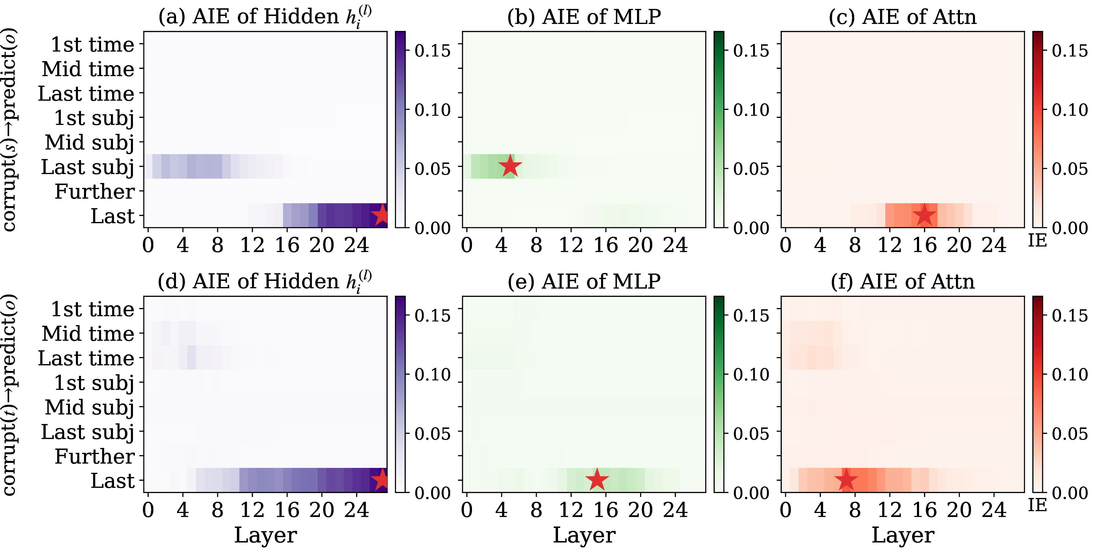
We apply the same procedure to GPT-J(6B). As shown in Figure 4, the temporal pathway consistently activates at earlier layers than the subject pathway, corroborating the findings on LLaMA-3 reported in §3.
9 Dataset Details↩︎
9.1 TimeConflict↩︎
9.1.1 Dataset Construction↩︎
We construct TimeConflict from the Wikidata JSON dump (latest-all.json.bz2). We extract temporal triples for 100 candidate properties using qualifier timestamps (P580 start-time, P582 end-time, P585
point-in-time), group them by subject, and detect temporal conflicts—pairs where after_object starts after the cutoff (January 1, 2023) and before_object is its most recent predecessor with a different identity. After removing
records with missing labels and deduplicating by (before_object, after_object, after_start), 24 properties yield \(\geq\)10 valid conflicts each, producing 22,708 records in total. For
TimeCF-Fictional, we replace each after_object with a random entity from the same-relation entity pool (seed = 42), preserving original timestamps.
9.1.2 Dataset Statistics↩︎
Table 4 summarizes the key statistics of TimeConflict. The per-relation record counts and sampling distribution are detailed in Table ¿tbl:tab:sampled95dist?. The distribution is long-tailed—the top 3 relations account for approximately 72% of all records, reflecting real-world knowledge update frequency.
| Statistic | Value |
|---|---|
| Total records | 22,708 |
| Relations | 24 |
| Unique subjects | \(>\)18,000 |
| Granularity | Day-level |
| Cutoff date | 2023-01-01 |
| Before-object range | 1751-09 – 2024-12 |
| After-object range | 2023-01 – 2025-12 |
| Experiment sample | 1,000 |
3pt
@llrr@ ID & Relation & #Samp. & #Full
P108 & employer & 231 & 8,747
P39 & position held & 145 & 5,538
P361 & part of & 74 & 75
P276 & location & 70 & 70
P35 & head of state & 66 & 66
P54 & member of sports team & 57 & 2,167
P710 & participant & 49 & 49
P102 & political party & 44 & 44
P166 & award received & 40 & 1,519
P449 & original broadcaster & 35 & 35
P131 & admin.territorial entity & 32 & 1,236
P286 & head coach & 28 & 1,082
P26 & spouse & 25 & 25
P749 & parent organization & 17 & 17
P793 & significant event & 16 & 600
P551 & residence & 14 & 14
P6 & head of government & 12 & 467
P355 & child organization & 12 & 12
P161 & cast member & 10 & 10
P488 & chairperson & 9 & 356
P69 & educated at & 4 & 165
P463 & member of & 4 & 167
P527 & has part(s) & 3 & 123
P1037 & director / manager & 3 & 124
& 1,000 & 22,708
9.1.3 Experiment Sampling Strategy↩︎
For our main experiments, we sample 1,000 records from the full dataset. Relations with fewer than 100 records (14 relations, 431 records) are included entirely; the remaining 569 slots are allocated proportionally among the 10 larger relations. Within
each large relation, we apply time-stratified sampling (40% newest, 30% middle, 30% oldest by after_object start date) to ensure temporal diversity. We filter out records with empty labels or identical before/after objects. All sampling uses
seed = 42. Table ¿tbl:tab:sampled95dist? shows the resulting distribution.
9.1.4 Data Examples↩︎
Below we show a TimeCF-Factual record and its TimeCF-Fictional counterpart. The Fictional variant is obtained by replacing after_object with a random entity from the
same-relation pool while keeping all other fields unchanged.
id: 341
relation: P6 (head of government)
subject: Toronto (Q172)
before_object: John Tory
time_range: 2014-12-01 to 2023-02-15
after_object: Olivia Chow
time_range: 2023-07-12 to ...
id: 341
relation: P6 (head of government)
subject: Toronto (Q172)
before_object: John Tory
time_range: 2014-12-01 to 2023-02-15
after_object: Thomas Müller
time_range: 2023-07-12 to ...
9.1.5 Comparison with Existing Datasets↩︎
Table 5 compares TimeConflict with existing knowledge editing datasets. Our dataset is the first to provide day-level temporal granularity with both factual and counterfactual variants.
| Dataset | Source | #Rec. | #Rel. | Granul. | CF |
|---|---|---|---|---|---|
| CounterFact [3] | Wikidata | 21,919 | 32 | None | ✔ |
| MQuAKE [23] | Wikidata | 3,000 | 37 | None | ✔ |
| ConflictBank [24] | Wikidata | 553K | – | Year | – |
| AToKe [7] | YAGO3.0 | 8,820 | 13 | Year | – |
| TimeCF (Ours) | Wikidata | 22,708 | 24 | Day | ✔ |
1.5pt
9.2 CounterFact\(^{\dagger}\) Augmentation↩︎
The original CounterFact [3] is a static counterfactual knowledge-editing benchmark; we refer readers to the original paper for its full construction protocol. In this work, we use it as the basis for CounterFact\(^{\dagger}\), a temporalized counterpart that keeps the original subject–relation–object rewrite semantics but adds an explicit historical/current distinction. This lets us test whether an editing method can introduce temporal conditioning into facts that are not temporal in the original benchmark.
9.2.1 Augmentation Protocol↩︎
9.2.1.1 Relation filtering.
We first restrict the original relations to a subset of 12 time-sensitive relations (e.g., occupation, employer, head of state, head of government, position held), keeping records where assigning the old and new answers to different time periods is semantically meaningful. This yields 6,219 records from the original 21,919.
9.2.1.2 Temporal augmentation.
We augment each filtered CounterFact record into a two-period contrast. The original answer is preserved in historical contexts, while the counterfactual target is assigned to current contexts. This turns a static subject–relation rewrite into a temporal editing case: a successful method must produce different answers for the same subject–relation pair depending on the temporal context. To reduce reliance on any single wording, we instantiate the historical/current contrast with several semantically equivalent temporal expressions (e.g., Since/Before, From \(\ldots\) onward/Prior to, As of/Up to).
9.2.2 Data Example↩︎
Below we show an original CounterFact record and its CounterFact\(^{\dagger}\) counterpart. The augmented variant converts the static rewrite into a two-period temporal contrast.
id: 18329
relation: occupation
subject: William Hardy Wilson
true_object: architect
counterfactual_target: journalist
edit: architect \(\rightarrow\) journalist
id: 18329
relation: occupation
subject: William Hardy Wilson
before_object: architect
time_context: “Prior to 2027, the occupation of William Hardy Wilson was”
after_object: journalist
time_context: “From 2027 onward, the occupation of William Hardy Wilson has been”
9.2.3 Scope and Complementarity↩︎
CounterFact\(^{\dagger}\) is a synthetic temporalization of CounterFact [3], the most widely adopted benchmark in the knowledge editing literature. By extending it to the temporal setting, we can evaluate our method on a well-established and broadly recognized data source, strengthening the comparability and credibility of our results. It complements TimeCF: TimeCF evaluates naturally occurring temporal changes, while CounterFact\(^{\dagger}\) tests whether a method can impose temporal distinctions on originally static facts. For our main experiments, we sample 1,000 records from CounterFact\(^{\dagger}\).
| Dataset | Method | CES\(\uparrow\) | CES-P\(\uparrow\) | CRS\(\uparrow\) | HES\(\uparrow\) | HES-P\(\uparrow\) | TC\(\uparrow\) |
|---|---|---|---|---|---|---|---|
| Pre-Edit | |||||||
| 2-8 | Fine-Tuning | ||||||
| ROME | |||||||
| CounterFact\(^{\dagger}\) | MEMIT | ||||||
| AlphaEdit | |||||||
| METO | |||||||
| PRISM Edit | |||||||
| Pre-Edit | |||||||
| 2-8 | Fine-Tuning | ||||||
| ROME | |||||||
| TimeCF-Factual | MEMIT | ||||||
| AlphaEdit | |||||||
| METO | |||||||
| PRISM Edit | |||||||
| Pre-Edit | |||||||
| 2-8 | Fine-Tuning | ||||||
| ROME | |||||||
| TimeCF-Fictional | MEMIT | ||||||
| AlphaEdit | |||||||
| METO | |||||||
| PRISM Edit |
| Dataset | Method | CES\(\uparrow\) | CES-P\(\uparrow\) | CRS\(\uparrow\) | HES\(\uparrow\) | HES-P\(\uparrow\) | TC\(\uparrow\) |
|---|---|---|---|---|---|---|---|
| Pre-Edit | |||||||
| 2-8 CounterFact\(^\dagger\) | GRACE | ||||||
| WISE | |||||||
| PRISM Edit | |||||||
| Pre-Edit | |||||||
| 2-8 TimeCF-Factual | GRACE | ||||||
| WISE | |||||||
| PRISM Edit | |||||||
| Pre-Edit | |||||||
| 2-8 TimeCF-Fictional | GRACE | ||||||
| WISE | |||||||
| PRISM Edit |
10 Additional Experimental Results↩︎
10.1 GPT-J Results↩︎
GPT-J-6B [19] is a widely used benchmark model in the knowledge editing literature. We replicate the main experiment (§5) on it to test cross-architecture generalization; only the editing layers are re-selected via causal tracing. As shown in Table 6, PRISM Edit achieves the best overall performance across multiple datasets, with particularly strong gains on CRS, confirming that temporal-polysemy editing transfers across architectures.
| Dataset | Method | CES\(\uparrow\) | CES-P\(\uparrow\) | CRS\(\uparrow\) | HES\(\uparrow\) | HES-P\(\uparrow\) | TC\(\uparrow\) |
|---|---|---|---|---|---|---|---|
| Pre-Edit | |||||||
| 2-8 CounterFact\(^\dagger\) | GRACE | ||||||
| WISE | |||||||
| PRISM Edit | |||||||
| Pre-Edit | |||||||
| 2-8 TimeCF-Factual | GRACE | ||||||
| WISE | |||||||
| PRISM Edit | |||||||
| Pre-Edit | |||||||
| 2-8 TimeCF-Fictional | GRACE | ||||||
| WISE | |||||||
| PRISM Edit |
| Model | Method | Time (s)\(\downarrow\) |
|---|---|---|
| LLaMA-3 | GRACE | 8.06 |
| WISE | 25.86 | |
| PRISM Edit | 5.44 | |
| GPT-J | GRACE | 27.22 |
| WISE | 20.87 | |
| PRISM Edit | 3.33 |
10.2 Memory-Based Methods (Llama-3 & GPT-J)↩︎
Although PRISM Edit primarily focuses on parameter-modifying editing on the MLP pathway analyzed in §3, we also compare against representative memory-based editors to position our method within the broader knowledge-editing landscape. We select GRACE [10] and WISE [11] as representative baselines: GRACE attaches an external key–value codebook and retrieves a stored value when the input matches a cached key, while WISE introduces a parametric side memory together with a router that decides whether to read from the main FFN or the side memory. Since both mechanisms operate outside the MLP pathway and follow a fundamentally different design principle from parameter-modifying editors, we report them separately.
Tables 7 and 8 present the full comparison. Methods of this type perform reasonably on direct-evaluation metrics (CES, HES, TC), but still exhibit a clear gap on the paraphrase-robust counterparts CES-P and HES-P. We view this difference as reasonable: such approaches deliberately leave the original model parameters intact and instead allocate extra memory or auxiliary modules to host the edited knowledge, so their behavior on unseen inputs is largely determined by how well those inputs are matched against the cached entries. In contrast, PRISM Edit performs parametric editing directly on the MLP pathway analyzed in §3, and consistently leads on CES-P, HES-P, and the integrated temporal-consistency score CRS, with the advantage being especially stable on paraphrase-robust metrics. Table 9 further shows that PRISM Edit also maintains a clear efficiency advantage, with a lower average per-record edit time than both GRACE and WISE.
10.3 Ablation on Context Templates↩︎
In MEMIT [4], the target value vector is optimized by averaging over \(P\) random prefix contexts prepended to the templated prompt, encouraging the edit to generalize beyond a single surface form. Since PRISM Edit already jointly optimizes \(v^*\) over multiple temporal conditions, this multi-condition diversity may subsume the role of random prefixes. We test this hypothesis by fixing \(\lambda_\text{old}{=}\lambda_\text{bare}{=}2\) and varying the number of paraphrased context templates per temporal condition from 1 to 10.
| # ctx | CES | CES-P | HES | HES-P | CRS | TC |
|---|---|---|---|---|---|---|
| 1 | 79.0 | 55.0 | 72.0 | 54.0 | 74.0 | 59.0 |
| 2 | 80.0 | 59.0 | 65.0 | 45.0 | 78.0 | 52.0 |
| 3 | 77.0 | 52.0 | 68.0 | 48.0 | 79.0 | 57.0 |
| 6 | 74.0 | 50.0 | 64.0 | 48.0 | 75.0 | 49.0 |
| 10 | 71.0 | 45.0 | 64.0 | 43.0 | 80.0 | 49.0 |
4pt
Results confirm this hypothesis. Increasing templates from 1 to 2 marginally improves CES/CES-P, yet degrades historical retention (HES/HES-P) and overall TC. At 10 templates, CRS peaks but TC drops by 10 points. The single-template default achieves the best overall balance (72.0/54.0/59.0 on HES/HES-P/TC), indicating that PRISM Edit’s multi-condition objective already provides sufficient optimization diversity—additional prefix augmentation only dilutes the temporal signal at the write site.
10.4 Case Study↩︎
| Panel | Example query |
|---|---|
| (a) Case 1 | “The political party of Kiyoshi Ueda is” |
| (b) Case 2 | “Óscar López-Pérez is employed by” |
| (c) Case 3 | “Rajneesh Choubisa is employed by” |
| (d) Case 4 | “Luis Gregory Gutierrez Zamalloa is employed by” |
| (e) Case 5 | “The award received by Pierre de Bousquet de Florian is” |
| (f) Case 6 | “A subsidiary of SoftBank Group is” |
| (g) Fail Case 1 | “Kentaro Tsukamoto is employed by” |
| (h) Fail Case 2 | “Batuhan Turhan Bozkurt is employed by” |
4pt
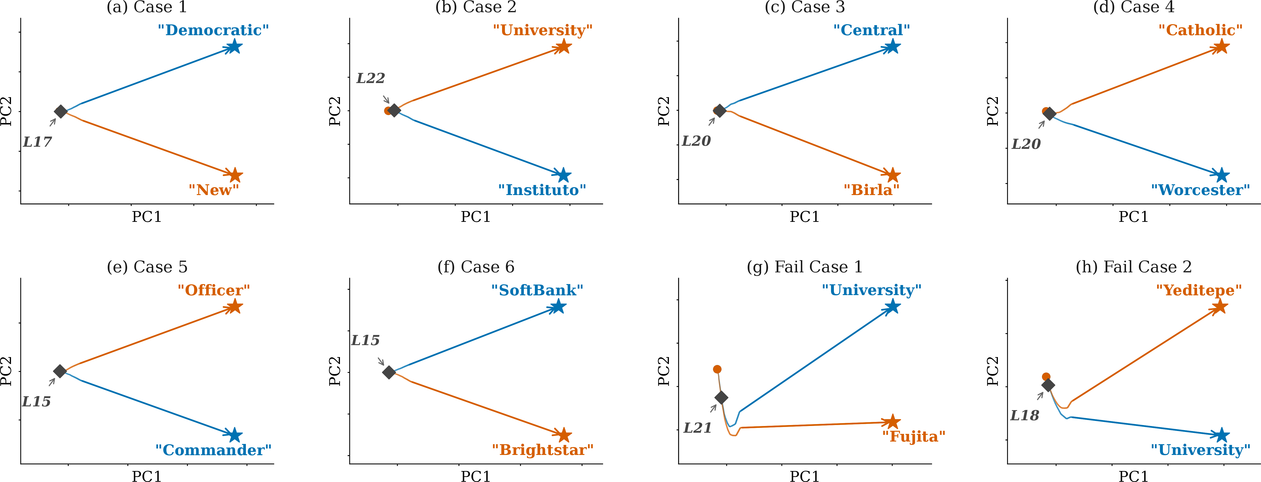
To visualize how PRISM Edit operates at the individual-record level, we conduct a case study on the post-edit model: for the same subject, we issue two queries that differ only in their temporal token (new-time and old-time), extract the last-token hidden states across all 32 layers, and project the two 32-layer trajectories onto their joint top-2 principal components. By design, after a single \(\boldsymbol{v}^{*}\) is written into the MLP, the model’s own temporal-modulation pathway should route the deep-layer readout to time-appropriate answers. Below we randomly sample six successful (Case 1–Case 6) and two failed cases (Fail Case 1, Fail Case 2) for comparative inspection; the corresponding queries are listed in Table 11.
In the six successful cases shown in Figure 5, the two trajectories overlap in the early layers—where representations encode syntax and entity identity—and then diverge in the later layers toward distinct attractors corresponding to the respective target answers. Each subplot marks its divergence onset layer with a diamond marker. Note that on the PCA plane the marker may visually appear close to the trajectory origin: this is because the early ten-plus layers carry essentially shared representations (the two queries share everything but a single temporal token), not because the divergence starts from \(L_0\). Across the six cases the onset ranges from \(L_{17}\) to \(L_{23}\) (mean \(\approx L_{20}\)), and the separation accelerates markedly from \(L_{23}\) onward, reaching its maximum at the final layer. This bifurcation pattern is consistent with the intended mechanism: a single polysemous value \(\boldsymbol{v}^{*}\) is written into the MLP, and the model’s existing temporal-modulation pathway routes the readout to time-appropriate answers without requiring separate edits for each time condition.
Figure 5 further shows two failure cases. The trajectory shape differs noticeably from the successful cases: instead of fanning out from a single shared bifurcation point, the two curves travel along a common arc for an extended span before separating, with one branch reaching the target and the other landing on a semantically adjacent but non-target entity. We tentatively attribute this to insufficient refinement within the remaining depth after a coarse routing has been completed, and leave a rigorous test to future work.
Overall, these visualizations provide qualitative evidence that PRISM Edit induces a layer-wise bifurcation in representation space starting around \(L_{20}\), consistent with the polysemous-value mechanism: a single \(\boldsymbol{v}^{*}\) writes a multi-valued payload into the MLP and the model’s existing temporal-modulation pathway routes the deep-layer readout to the appropriate time.
11 PRISM Edit Algorithm↩︎
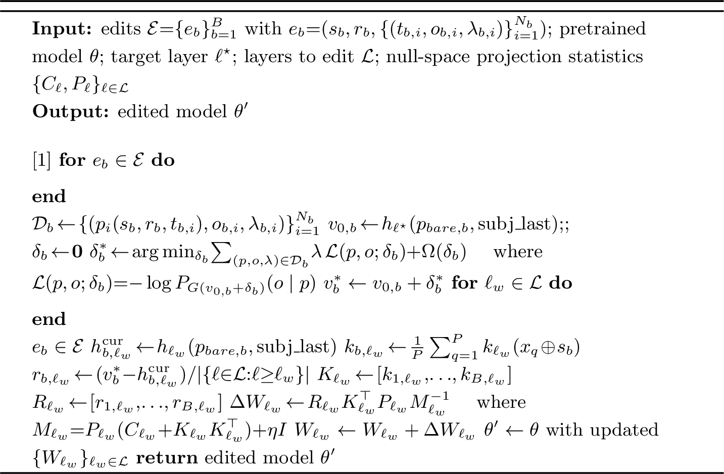
Notation. \(h_\ell(p,t)\in\mathbb{R}^d\) denotes the hidden state at layer \(\ell\) and token position \(t\) for input \(p\). The target layer \(\ell^\star\) is where the polysemous value \(\boldsymbol{v}^\ast\) is optimized, and \(\mathcal{L}\) is the set of layers to edit. For edit \(b\), \(p_{\text{bare},b}\) is the bare prompt built from \((s_b, r_b)\) without temporal tokens, \(\mathrm{subj\_last}\) marks the last-subject-token position, and \(\lambda_{b,i}\) weights the \(i\)-th target pair \((t_{b,i}, o_{b,i})\). The key \(k_\ell(\cdot)\) is the MLP key at layer \(\ell\), averaged over random context templates \(\{x_q\}_{q=1}^{P}\). Finally, \(C_\ell\) and \(P_\ell\) are the pre-computed key covariance and null-space projector at layer \(\ell\), and \(\eta\) is the L2 regularization coefficient.
References↩︎
Code and data: https://github.com/Cheer-Huang/PRISM-Edit↩︎