1 Introduction↩︎

1.0.0.1 (Extended) MFC.

(Extended) mean field control (MFC) provides a tractable framework for large population stochastic games, by optimizing the collective behavior of homogeneous and interacting agents through a central planner [1]. In the mean-field limit, the controlled state of a (representative) agent is governed by a McKean-Vlasov system \[\begin{align} \label{eq:intro95MV} \begin{aligned} {\mathrm{d}}X^{\alpha}_s =b(s,X^{\alpha}_s, {\alpha}_s, \mathbb{P}_{(X^{\alpha}_s, {\alpha}_s)}){\mathrm{d}}s+\sigma(s,X^{\alpha}_s, {\alpha}_s, \mathbb{P}_{(X^{\alpha}_s, {\alpha}_s)}){\mathrm{d}}W_s, \end{aligned} \end{align}\tag{1}\] where both the drift and diffusion coefficients depend on the distribution of the state \(X^{\alpha}\) and the control \({\alpha}\). Although this limit removes the explicit dependence on the number of agents, the associated extended MFC is intrinsically an infinite-dimensional control problem: the value function and the optimal feedback generally depend not only on time and the individual state, but also on the state distribution. The most fundamental theoretical ingredients in the development of MFC theory are the dynamic programming principle for the lifted value function defined on the space of probability measures, and the invariance property of this value function along the deterministic state flow (see e.g., [2], [3]).

1.0.0.2 Continuous-time RL with deterministic policy.

In extended mean field control, both the dynamics and reward may depend on the joint distribution of states and controls. To address this challenge, we adopt deterministic feedback policies. A deterministic policy \(\varphi(t,x,\mu)\) selects an action directly based on the current time, state and state law, so that the state law together with the feedback map completely determines the associated state–action distribution through the push-forward measure \(\Gamma_t^{\varphi}= \bigl(\operatorname{id},\varphi(t,\cdot,\mu_t)\bigr)_{\#}\mu_t,\) with \(\mu_t\) being the current state distribution. For continuous-time reinforcement learning (RL), recent analysis using deterministic policies [4], [5] have shown superiority over both the discretization approach and the stochastic policies. Analytically, the state–action distribution is induced directly as a push-forward of the state law. Hence the policy optimization over controls is reduced to an optimization over a parameterized family of deterministic policies \(\varphi_{\theta}\) (with respect to parameter \(\theta\)). Numerically, deterministic policies have also been shown to offer improved computational efficiency and greater stability [4].

1.0.0.3 Learning for discrete-time MFC.

In the RL framework of MFCs, the agent does not know the state coefficients \(b\) and \(\sigma\), nor the reward functions, and instead, learns by interacting with the controlled system. In discrete time, dynamic programming principles have been established for both state- and state-action value functions, leading to value-based algorithms including Q-learning and integrated Q-functions based on local policies [6]–[8]. More recently, model-free policy-gradient methods have also been proposed in [9], culminating in the MF-REINFORCE algorithm with theoretical guarantees on the bias and variance of the policy-gradient estimator.

1.0.0.4 Our work for continuous-time extended MFC.

This paper develops an RL framework for continuous-time extended MFC, adopting the deterministic policy approach.

We first develop a model-free deterministic policy gradient formula for continuous-time extended MFC (Theorem 4). This representation expresses the gradient of value function with respect to the policy parameter as an integral involving the derivative of an advantage-rate function along the flow of state distributions. This advantage-rate function is lifted to a function on the space of probability measures and is characterized jointly with the value function through an invariance principle along the flow of state distributions. These results are derived using a model-free sensitivity formula for parametric McKean–Vlasov dynamics (Theorems 1 and 3), which relies on a performance difference lemma (Lemma 6) and the robustness of the state distribution with respect to model parameters. These results for continuous-time extended MFC are consistent with their discrete-time counterpart regarding lifted (state–action) value functions and Q-functions [6]–[8].

We then refine the deterministic policy gradient formula by explicitly accounting for its dependence on the joint state–action distribution (Theorem 5). Specifically, we decompose the lifted value function and the lifted advantage-rate function into integrals of local functions of the state, action, and the joint state–action distribution. The resulting policy gradient contains both the usual derivative of the local advantage-rate function with respect to the individual action and an additional measure-derivative term with respect to control distribution. We further establish a martingale characterization to learn these local representations directly from observed state and control trajectories. Just as the incorporation of local policies facilitates efficient learning in the discrete-time MFC [8], this local advantage-rate function allows more informative learning than directly learning from the flow of state laws (Section 4). This approach applies to general extended MFC problems, and removes the restrictive assumption in [10] which requires a separable structure on the coefficients and explicit and known dependence on the control variable.

Finally, we propose a continuous-time deep deterministic policy-gradient algorithm for extended MFC. The algorithm combines measure-dependent neural networks, particle approximations of the McKean-Vlasov dynamics, temporal-difference learning based on the aforementioned martingale characterization, and action- or parameter-space exploration. The use of finite-dimensional distribution embeddings is consistent with the neural approximation principles developed in [11], [12], while the deterministic actor avoids direct optimization over a space of stochastic kernels. Numerical experiments for consensus control in a stochastic Cucker-Smale system and optimal liquidation with mean-field market impact demonstrate the efficiency and robustness of the proposed method, including in settings where the dynamics depend explicitly on the distribution of the control.

1.0.0.5 Earlier work for RL in continuous-time-space MFC.

Many earlier studies on continuous-time MFC reinforcement-learning have been built on stochastic, or exploratory, policies; and focuses on the setting where the coefficients depend only on the law of the state process. In this exploratory formulation, the admissible policy class is enlarged to stochastic policies that map the time, state, and state distribution to a probability measure over the action space. However, RL algorithms under the exploratory control formulation appear too restrictive for the infinite-dimensional nature of MFC. For example, in [10], the state coefficients are required to possess a separable structure, and the explicit dependence on the control variable must be known in order to characterize the mean-field \(q\)-function. In [13], [14], algorithms require learning two \(q\)-functions: an integrated \(q\)-function identified via weak martingale conditions by testing against all stochastic policies, and an essential \(q\)-function used for policy improvement. In [15], the exploratory HJB equation contains an additional nonlinear functional of the policy, and the optimal policy is characterized by a two-layer fixed-point problem over the space of stochastic policies. The corresponding algorithms in [16] then face the issue that data generated by the relaxed-control formulation are not directly observable, requiring additional approximation by discretely sampled exploratory actions, as in [17], [18].

To see analytically the fundamental obstacle of stochastic-policy methods for learning extended MFC, consider a stochastic Markov policy \(\pi(\mathrm{d}a | t,x,\mu)\) and its induced state-action distribution \(\Gamma_t^{\pi}(\mathrm{d}x,\mathrm{d}a) = \bigl(\operatorname{id}, \pi(\mathrm{d}a | t,\cdot,\mu_t) \bigr)_{\#}\mu_t\). In a standard MFC problem whose coefficients depend only on the state distribution, stochastic policies produce an auxiliary generator by integrating the original state generator over the action space with respect to the stochastic policy \(\pi\), which is linear in the stochastic policy. This linearity is central for stochastic-policy based algorithms [10], [19], [20]. When applying the exploratory control formulation to extended MFC, randomizing actions through relaxed controls necessarily alters the control distribution \(\mathbb{P}_{\alpha_t}\) in (1 ), so that the action randomization can no longer be separated from the interaction induced by the control distribution. Thus, one cannot derive an auxiliary dynamics whose generator depends linearly on the stochastic policy.

In fact, stochastic policies face algorithmic challenges even in the single-agent setting. They require sampling random actions at very high frequency, leading to irregular control trajectories that may be impractical in real-world applications [16]–[18]. Moreover, the Bellman equation under stochastic policies involves integration over continuous action spaces. Enforcing this condition requires Monte Carlo approximation, which is computationally expensive and often leads to unstable and slow convergence.

In contrast, the benefit of deterministic policies for MFC is clear: the state–action distribution is induced directly as a push-forward of the state law. It avoids optimization over stochastic kernels, helps bypass key limitations of exploratory-policy approaches in extended mean field settings, and facilitates policy updates by differentiating through both the selected actions and the induced state–action distributions. As demonstrated in [4] for single-agent RL problems and the numerical experiments in this paper, deterministic policies offer significant computational advantages in continuous-time-space settings, leading to model-free algorithms with improved stability and faster convergence compared with stochastic-policy methods.

1.0.0.6 Notation.

We denote by \(x\cdot y\) the scalar product between two vectors \(x\in {\mathbb{R}}^m\) and \(y\in {\mathbb{R}}^m\), and by \(M\colon N=\mathop{\mathrm{tr}}(M^\top N)\) the inner product between two matrices \(M\in {\mathbb{R}}^{m\times n}\) and \(N\in {\mathbb{R}}^{m\times n}\).

Given \(T>0\), a filtered probability space \((\Omega, \mathcal{F}, \mathbb{F}=(\mathcal{F}_t)_{t\in [0,T]}, \mathbb{P})\), a normed space \((E, |\cdot|)\), and an \(E\)-valued random variable \(X\) on \((\Omega, \mathcal{F}, \mathbb{P})\), we denote by \(\mathbb{P}_X\) its probability law under \(\mathbb{P}\), by \(X\sim \mu\) the fact that \(X\) follows the distribution \(\mu\), by \({\mathbb{E}}_{\xi\sim \mu}[f(\xi)]=\int_E f(x)\mu ({\mathrm{d}}x)\) for a measurable function \(f:E\to {\mathbb{R}}\), and by \(L^2(\mathcal{F}_t; E)\) the set of square integrable \(E\)-valued random variables on \((\Omega, \mathcal{F}_t,\mathbb{P})\) for all \(t\in [0,T]\). We denote by \(\mathcal{P}_2(E)\) the set of probability measures \(\mu\) on \(E\) that are square integrable, i.e., \(M_2(\mu) \mathrel{\vcenter{:}}= \left(\int_E |x|^2 \mu(dx)\right)^{1/2} < \infty.\) We shall assume without loss of generality that \(\mathcal{F}_0\) is rich enough to carry \(E\)-valued random variables with any square integrable distribution, i.e., \(\mathcal{P}_2(E) = \{ \mathbb{P}_\xi \mid \xi \in L^2(\mathcal{F}_0; E) \}.\) We equip \(\mathcal{P}_2(E)\) with the 2-Wasserstein distance \(\mathcal{W}_2\) defined by \[\begin{align} \mathcal{W}_2(\mu, \mu') &= \inf \left\{ \left( \int_{E \times E} |x - y|^2 \, \pi(dx, dy) \right)^{1/2} \,\bigg\vert\, \pi \in \mathcal{P}_2(E \times E) \text{ with marginals } \mu \text{ and } \mu' \right\} \\ &= \inf \left\{ \left( \mathbb{E} \left[ |\xi - \xi'|^2 \right] \right)^{1/2} \,\Big\vert\, \xi, \xi' \in L^2(\mathcal{F}_0; E), \, \mathbb{P}_\xi = \mu, \, \mathbb{P}_{\xi'} = \mu' \right\}. \end{align}\]

We denote by \(C^{1,2}([0, T]\times \mathcal{P}_2(\mathbb{R}^n))\) the space of continuous functions \(w : [0, T] \times \mathcal{P}_2(\mathbb{R}^n) \to \mathbb{R}\) such that for all \(\mu\in \mathcal{P}_2({\mathbb{R}}^n)\), \(w(\cdot, \mu)\) is \(C^{1}([0,T])\), with \(\partial_t w\) being continuous in all variables; for all \(t\in [0,T]\), \(w(t,\cdot)\) is L-differentiable, and \((t,\mu,v)\mapsto \partial_\mu w(t,\mu)(v)\) is continuous at all \((t,\mu,v)\) with \(v\in \operatorname{supp}(\mu)\); for all \((t,\mu)\in [0,T]\times \mathcal{P}_2({\mathbb{R}}^n)\), \(\partial_\mu w(t,\mu)(\cdot)\) is \(C^1\), with \((t,\mu, v) \mapsto \partial_v \partial_\mu w(t,\mu)(v)\) being continuous at all \((t,\mu,v)\) with \(v\in \operatorname{supp}(\mu)\); and for all compact sets \(\mathcal{K}\subset \mathcal{P}_2({\mathbb{R}}^n)\), \[\sup_{(t,\mu) \in [0,T]\times \mathcal{K}}\left[\int_{{\mathbb{R}}^n} |\partial_\mu w(t, \mu) (\xi)|^2\mu ({\mathrm{d}}\xi) +\|\partial_v \partial_\mu w(t,\mu)\|_{L^\infty_\mu} \right]<\infty.\]

2 Model-free sensitivity formula of McKean-Vlasov dynamics↩︎

This section considers a multidimensional McKean–Vlasov dynamics parameterized by \(\theta\) and derives model-free representations of the gradient of the value functional with respect to \(\theta\). Consistent with the existing literature on MFCs, we consider the lifted value function defined on the Wasserstein space of probability measures. The derivation of these representations exploits both the invariance property of the value function and the robustness of the state distribution with respect to the model parameters. These representations will be useful for developing learning algorithms for the controlled McKean-Vlasov dynamics in Section 3.

Let \(T>0\) be a given terminal time, and \((\Omega, \mathcal{F}, \mathbb{P})\) be a probability space on which an \(m\)-dimensional Brownian motion \(W = (W_t)_{0 \leq t \leq T}\) is defined. We denote by \(\mathbb{F} = (\mathcal{F}_t)_{0 \leq t \leq T}\) the filtration generated by \(W\), augmented with \(\mathbb{P}\)-null sets, and assume that the initial \(\sigma\)-algebra \(\mathcal{F}_0\) is rich enough. Let \(\beta\ge 0\) be a discount factor, and consider continuous functions \(b:[0,T]\times {\mathbb{R}}^n\times \mathcal{P}_2( {\mathbb{R}}^n)\times {\mathbb{R}}^k\to {\mathbb{R}}^n\), \(\sigma:[0,T]\times {\mathbb{R}}^n\times \mathcal{P}_2( {\mathbb{R}}^n)\times {\mathbb{R}}^k\to {\mathbb{R}}^{n\times m}\), \(r:[0,T]\times {\mathbb{R}}^n\times \mathcal{P}_2( {\mathbb{R}}^n)\times {\mathbb{R}}^k\to {\mathbb{R}}\) and \(g:{\mathbb{R}}^n\times \mathcal{P}_2({\mathbb{R}}^n)\to {\mathbb{R}}\) satisfying the following regularity and growth conditions:

For each \(t\in [0,T]\), \(\theta\in {\mathbb{R}}^k\), and \(\xi\in L^2(\mathcal{F}_t; {\mathbb{R}}^n)\), consider the following state dynamics: \[\begin{align} {\mathrm{d}}X^{t, \xi,\theta}_s &=b(s,X^{t, \xi, \theta}_s, \mathbb{P}_{X^{t, \xi,\theta}_s}, \theta){\mathrm{d}}s+\sigma(s,X^{t, \xi,\theta}_s, \mathbb{P}_{X^{t, \xi, \theta}_s}, \theta){\mathrm{d}}W_s, \quad s\in [t,T]; \quad X^{t, \xi,\theta}_t=\xi. \label{eq:sde95mv95population} \end{align}\tag{2}\] Under Assumption 1, (2 ) has a unique square-integrable strong solution \((X^{t, \xi,\theta}_s)_{s\in [t,T]}\) (see e.g., [2] and the references therein). Moreover, due to the weak uniqueness of (2 ), the law of \((X^{t, \xi,\theta}_s)_{s\in [t,T]}\) depends on \(\xi\) only through its law \(\mu=\mathbb{P}_{\xi}\), and hence we can define \[\mathbb{P}^{t,\mu,\theta}_s\mathrel{\vcenter{:}}= \mathbb{P}_{X^{t,\xi, \theta}_s}, \quad s\in [t,T].\] Define the following value function for a given \(\beta\ge 0\): \[\begin{align} \label{eq:cost95theta} V(t,\mu,\theta) &\mathrel{\vcenter{:}}= {\mathbb{E}}\left[ \int_t^T e^{-\beta (s-t)} r\left(s, X^{t,\xi, \theta}_s, \mathbb{P}_{{X^{t,\xi, \theta}_s}}, \theta\right) {\mathrm{d}}s + e^{-\beta (T-t)} g\left(X^{t,\xi, \theta}_T, \mathbb{P}_{X^{t,\xi, \theta}_T}\right) \right] \\ &= \int_t^T e^{-\beta (s-t)} \bar r \left(s, \mathbb{P}^{t,\mu,\theta}_s, \theta\right) {\mathrm{d}}s + e^{-\beta (T-t)} \bar g ( \mathbb{P}^{t,\mu,\theta}_T ), \end{align}\tag{3}\] where the function \(\bar r: [0,T]\times \mathcal{P}_2({\mathbb{R}}^n)\times {\mathbb{R}}^k\to {\mathbb{R}}\) and \(\bar g:\mathcal{P}_2({\mathbb{R}}^n)\to {\mathbb{R}}\) are defined by \[\bar r (t,\mu,\theta)\mathrel{\vcenter{:}}= \int_{{\mathbb{R}}^n} r(t,x,\mu,\theta) \mu({\mathrm{d}}x), \quad \bar g(\mu ) \mathrel{\vcenter{:}}= \int_{{\mathbb{R}}^n} g(x,\mu)\mu({\mathrm{d}}x).\]

To characterize the gradient of \(V\) in \(\theta\), for all \(w\in C^{1,2}([0,T]\times \mathcal{P}_2({\mathbb{R}}^n))\), define the function \(A[w]:[0,T]\times \mathcal{P}_2({\mathbb{R}}^n)\times {\mathbb{R}}^k \to {\mathbb{R}}\) such that for all \((t,\mu,\theta)\in [0,T]\times\mathcal{P}_2({\mathbb{R}}^n)\times {\mathbb{R}}^k\), \[\label{eq:advantage95rate} A[w](t,\mu,\theta)\mathrel{\vcenter{:}}= \mathcal{L}^{ \theta}[w] (t, \mu ) +\bar r(t,\mu,\theta),\tag{4}\] where \(\mathcal{L}^\theta\) is the generator of (2 ) given by \[\begin{align} \label{eq:generator} \begin{aligned} \mathcal{L}^\theta[ w](t, \mu) &\mathrel{\vcenter{:}}= \partial_t w(t, \mu) -\beta w(t, \mu) \\ &\quad+ {\mathbb{E}}_{\xi\sim\mu} \left[ b(t,\xi,\mu,\theta)\cdot \partial_\mu w(t, \mu) ( \xi) +\frac{1}{2} (\sigma\sigma^\top) (t,\xi,\mu,\theta)\colon \partial_v \partial_\mu w(t, \mu)(\xi) \right]. \end{aligned} \end{align}\tag{5}\] We impose the following regularity conditions on the value function \(V^\theta\) and the function \(A[w]\).

For all $w\in C^{1,2}([0,T]\times \mathcal{P}_2({\mathbb{R}}^n))$,
the function $A[w]$ defined by (@eq:eq:advantage95rate ) is
differentiable with respect to $\theta$, and the derivative
$\partial_\theta A[w] : [0,T]\times \mathcal{P}_2({\mathbb{R}}^n)\times {\mathbb{R}}^k\to {\mathbb{R}}^k$
is continuous.

Under Assumptions 1 and 2, the following theorem shows that the gradient \(\partial_\theta V\) can be expressed as the integral of \(\partial_\theta A\) in (4 ) along the flow of state laws.

Theorem 1 expresses the gradient \(\partial_\theta V\) directly in terms of \(\partial_\theta A [V]\), without reference to the model coefficients. The proof leverages a precise characterization of the difference between the value functions corresponding to two different parameters (Proposition 6). Such a result extends the performance-difference lemmas in [4] and [21] from classical control problems to the more general setting of McKean–Vlasov dynamics. Compared with existing approaches in [19], [22], our method avoids differentiating the PDE for the value function \(V(\cdot,\cdot,\theta)\) with respect to \(\theta\), and therefore requires weaker regularity assumptions on the coefficients. In particular, we do not require differentiability in \(\theta\) of the first- and second-order time and spatial derivatives of \(V\), which is imposed in [19].

To characterize the advantage rate function, we first show that the value function \(V\) and the advantage rate function \(A[V]\) must satisfy a Feynman-Kac formula and an invariance property along the deterministic state flow.

Conversely, we show that the conditions (?? ) and (?? ) are sufficient to jointly characterize both the value function \(V\) and the advantage rate function \(A[V]\). This derivation is based on two key properties in general MFC: the first being the invariance property of the value function for any given policy along the deterministic state flow in a neighborhood of \(\theta\), and the second being the continuity of the law of McKean–Vlasov systems with respect to the perturbations of the initial condition and model parameters.

For any given \(\theta\), Theorem 3 characterizes the associated value function and advantage rate function in a neighborhood of \(\theta\), via the Feynman–Kac formula (?? ) and the invariance principle (?? ) along deterministic state flows. This provides a unified framework for characterizing value and advantage functions under arbitrary policies, and applies to both deterministic policies as in Section 3 and stochastic policies as in [10], [14].

3 Deterministic Policy Gradient for Extended MFC Problems↩︎

In this section, we apply the sensitivity formula in Section 2 to derive a policy gradient formula for extended mean field control (MFC) problems studied in [1], [23]. In extended MFC problems, both the cost functional and the state dynamics depend on the joint distribution of the controlled state and control processes. This formula provides the foundation for developing a model-free deterministic actor–critic algorithm in Section 4 for solving extended MFC problems.

3.1 Problem formulation↩︎

3.1.0.1 Extended MFC problems.

Let \(T>0\) be a given terminal time and \((\Omega, \mathcal{F},\mathbb{P})\) be a complete probability space which supports an \(m\)-dimensional Brownian motion \(W\) and an independent square-integrable random variable \(\xi_0\). We denote by \(\mathbb{F} = (\mathcal{F}_t)_{t\ge 0}\) the filtration generated by \(W\) and \(\xi_0\) augmented by the \(\mathbb{P}\)-null sets. Let \(A\subset \mathbb{R}^d\) be a measurable set representing the agent’s action space, and let \(\mathcal{U}\) be a space of all \(\mathbb{F}\)-adapted square-integrable processes \(\alpha:[0,T]\times \Omega\to A\) representing the agent’s admissible control space.

For each \(\alpha\in \mathcal{U}\), consider the associated state process \(X^\alpha\) governed by the following controlled McKean-Vlasov dynamics: \[\begin{align} \label{eq:sde95mv95open95loop} \begin{aligned} {\mathrm{d}}X^{\alpha}_s =b(s,X^{\alpha}_s, {\alpha}_s, \mathbb{P}_{(X^{\alpha}_s, {\alpha}_s)}){\mathrm{d}}s+\sigma(s,X^{\alpha}_s, {\alpha}_s, \mathbb{P}_{(X^{\alpha}_s, {\alpha}_s)}){\mathrm{d}}W_s, \quad X^{\alpha}_0=\xi_0, \end{aligned} \end{align}\tag{6}\] where \(b:[0,T]\times {\mathbb{R}}^n \times {\mathbb{R}}^d \times \mathcal{P}_2({\mathbb{R}}^n\times {\mathbb{R}}^d)\to {\mathbb{R}}^n\) and \(\sigma:[0,T]\times {\mathbb{R}}^n \times {\mathbb{R}}^d \times \mathcal{P}_2({\mathbb{R}}^n\times {\mathbb{R}}^d)\to {\mathbb{R}}^{n\times m}\) are sufficiently regular functions such that (6 ) has a unique square-integrable strong solution \(X^\alpha\). The agent aims to maximize the following reward functional \[\begin{align} \label{eq:reward95mv95open95loop} J(\alpha) \mathrel{\vcenter{:}}= {\mathbb{E}}\left[ \int_0^T e^{-\beta s} r (s,X^{\alpha}_s, {\alpha}_s, \mathbb{P}_{(X^{\alpha}_s, {\alpha}_s)}) {\mathrm{d}}s + e^{-\beta T} g(X^{\alpha}_T, \mathbb{P}_{X^{\alpha}_T}) \right] \end{align}\tag{7}\] over all \(\alpha\in \mathcal{U}\), where \(\beta \ge 0\), \(r: [0,T]\times {\mathbb{R}}^n \times {\mathbb{R}}^d \times \mathcal{P}_2({\mathbb{R}}^n\times {\mathbb{R}}^d)\to {\mathbb{R}}\) and \(g:{\mathbb{R}}^n \times \mathcal{P}_2({\mathbb{R}}^n)\to {\mathbb{R}}\) are continuous functions with at most quadratic growth.

It is known that under suitable regularity conditions (see e.g., [2]), it suffices to optimize (7 ) over control processes \(\alpha^\varphi=(\alpha^\varphi_t)_{t\in [0,T]}\) given in closed loop (or feedback) form: \[\label{eq:alpha95feedback} \alpha^\varphi_t= \varphi(t,X^\varphi_t, \mathbb{P}_{X^\varphi_t}), \quad t\in [0,T],\tag{8}\] where \(\varphi: [0,T]\times {\mathbb{R}}^n\times \mathcal{P}_2({\mathbb{R}}^n)\to A\) is a measurable function, called a Markov policy, and \(X^\varphi\) is a solution to the following controlled McKean-Vlasov dynamics: \[\begin{align} \label{eq:sde95mv95cl} \begin{aligned} {\mathrm{d}}X^{\varphi}_s =& b(s,X^{\varphi}_s, \varphi(s,X^\varphi_s, \mathbb{P}_{X^\varphi_s}), \mathbb{P}_{(X^{\varphi}_s, \varphi(s,X^\varphi_s, \mathbb{P}_{X^\varphi_s}))}){\mathrm{d}}s \\ &+\sigma(s,X^{\varphi}_s, \varphi(s,X^\varphi_s, \mathbb{P}_{X^\varphi_s}), \mathbb{P}_{(X^{\varphi}_s, \varphi(s,X^\varphi_s, \mathbb{P}_{X^\varphi_s}))}){\mathrm{d}}W_s, \quad X^{\varphi}_0=\xi_0, \end{aligned} \end{align}\tag{9}\] Consequently, the goal of the agent is to maximize the following objective \[\begin{align} \label{eq:reward95mv95cl} J(\varphi) \mathrel{\vcenter{:}}= {\mathbb{E}}\left[ \int_0^T e^{-\beta s} r (s,X^{\varphi}_s, \varphi(s,X^\varphi_s, \mathbb{P}_{X^\varphi_s}), \mathbb{P}_{(X^{\varphi}_s, \varphi(s,X^\varphi_s, \mathbb{P}_{X^\varphi_s}))}) {\mathrm{d}}s + e^{-\beta T} g(X^{\varphi}_T, \mathbb{P}_{X^{\varphi}_T}) \right] \end{align}\tag{10}\] over all admissible Markov policies \(\varphi\).

3.1.0.2 RL with deterministic policies.

In the RL framework, the agent does not know the coefficients \(b,\sigma, r\) and \(g\). Instead, the agent interacts directly with the system (9 ) with different actions and updates her policies based on the observed state and reward trajectories.

As in the classical McKean-Vlasov control framework, we restrict attention to suitable Markov policies \(\varphi:[0,T]\times {\mathbb{R}}^n\times \mathcal{P}_2({\mathbb{R}}^n)\to A\) for optimizing (10 ). In the RL literature, such policies are referred to as deterministic policies, since they map each time-state-measure triple directly to an action. A deterministic feedback policy \(\varphi(t,x, \mu)\) selects an action directly based on the time \(t\), state \(x\) and law \(\mu\), and the associated state–action distribution is the push-forward measure \(\Gamma_t^{\varphi} = \bigl(\operatorname{id},\varphi(t,\cdot,\mu)\bigr)_{\#}\mu\) defined in (12 ). The joint distribution is therefore completely determined by the state law and the feedback map. Although the resulting dynamics may still depend nonlinearly on \(\Gamma_t^{\varphi}\), policy optimization can be reduced to an optimization over a parameterized family \(\varphi_{\theta}\).

More precisely, let \(\operatorname{Lip}([0,T]\times {\mathbb{R}}^n\times \mathcal{P}_2({\mathbb{R}}^n); A)\) be the set of continuous functions \(\varphi:[0,T]\times {\mathbb{R}}^n\times \mathcal{P}_2({\mathbb{R}}^n)\to A\) that are Lipschitz continuous in \((x,\mu)\), uniformly on \(t\in [0,T]\). Given a class of parameterized policies \(\mathscr P_\Theta \mathrel{\vcenter{:}}= \{\varphi_\theta \in \operatorname{Lip}([0,T]\times {\mathbb{R}}^n\times \mathcal{P}_2({\mathbb{R}}^n); A)\mid \theta\in {\mathbb{R}}^k\}\), we maximize the following functional over \(\theta\in {\mathbb{R}}^k\): \[\begin{align} \label{eq:dpg95cost95theta} J(\theta) \mathrel{\vcenter{:}}= {\mathbb{E}}\left[ \int_0^T e^{-\beta s} r (s,X^{\varphi_\theta}_s, {\varphi_\theta}(s,X^{\varphi_\theta}_s, \mathbb{P}_{X^{\varphi_\theta}_s}), \mathbb{P}_{(X^{\varphi_\theta}_s, {\varphi_\theta}(s,X^{\varphi_\theta}_s, \mathbb{P}_{X^{\varphi_\theta}_s}))}) {\mathrm{d}}s + e^{-\beta T} g(X^{\varphi_\theta}_T, \mathbb{P}_{X^{\varphi_\theta}_T}) \right], \end{align}\tag{11}\] where we write \(J(\theta) = J(\varphi_\theta)\) with a slight abuse of notation.

In the sequel, we propose model-free deterministic policy gradient (DPG) algorithms that optimize (11 ) via a gradient ascent algorithm.

3.2 Deterministic policy gradient formula↩︎

3.2.0.1 Reformulation as parametric McKean-Vlasov dynamics.

To compute \(\nabla_\theta J(\varphi_\theta)\) using Theorems 1 and 3, we rewrite (11 ) as a special case of the parametric McKean-Vlasov dynamics analyzed in Section 2. As in [2], for each policy \(\varphi \in \mathscr P_\Theta\) and \((t,\mu)\in [0,T]\times \mathcal{P}_2({\mathbb{R}}^n)\), let \((\mathop{\mathrm{\textrm{id}}}, \varphi (t,\cdot, \mu))_\sharp \mu\in \mathcal{P}_2( {\mathbb{R}}^n\times {\mathbb{R}}^d)\) be the induced state-action measure given by \[\begin{align} \label{eq:push95forward} [(\mathop{\mathrm{\textrm{id}}}, \varphi (t,\cdot, \mu))_\sharp \mu ](B)&\mathrel{\vcenter{:}}= \mu(\{x\in {\mathbb{R}}^n\mid (x,\varphi (t,x,\mu))\in B\}), \quad \forall B\in \mathcal{B}({\mathbb{R}}^n\times {\mathbb{R}}^d). \end{align}\tag{12}\] Note that for any control \(\alpha^\varphi\) of the form (8 ), the joint state-control distribution satisfies \[\mathbb{P}_{(X^{\varphi}_t, {\alpha}^\varphi_t)} =(\mathop{\mathrm{\textrm{id}}}, \varphi (t,\cdot, \mathbb{P}_{X^{\varphi}_t}))_\sharp \mathbb{P}_{X^{\varphi}_t}, \quad t\in [0,T].\] Define the following controlled coefficients associated with \(\mathscr P_\Theta\): for all \(\ell\in \{b,\sigma, r\}\), \[\begin{align} \label{eq:coefficient95mfc95dpg} \ell^\varphi (t, x, \mu,\theta) &\mathrel{\vcenter{:}}= \ell (t,x, \varphi_\theta(t,x,\mu), (\mathop{\mathrm{\textrm{id}}}, \varphi_\theta(t,\cdot, \mu))_\sharp \mu ). \end{align}\tag{13}\] The dynamics (9 ) with \(\varphi=\varphi_\theta\) can then be rewritten as \[\begin{align} \label{eq:dpg95state95psi95theta} \begin{aligned} {\mathrm{d}}X_s =& b^{\varphi}(s,X_s,\mathbb{P}_{X_s}, \theta) {\mathrm{d}}s +\sigma^{\varphi}(s,X_s,\mathbb{P}_{X_s}, \theta) {\mathrm{d}}W_s. \end{aligned} \end{align}\tag{14}\] Consider the dynamic version of (11 ) defined as follows (cf. (3 )) : for all \((t,\mu)\in [0,T]\times \mathcal{P}_2({\mathbb{R}}^n)\), let \(\xi\in L^2(\mathcal{F}_t;{\mathbb{R}}^n)\) with \(\mathbb{P}_{\xi}=\mu\) and \(X^{t,\xi,\theta}\) satisfy (14 ) on \([t,T]\) with \(X^{t,\xi,\theta}_t=\xi\), and define \[\begin{align} \label{eq:V95varphi95theta} V^\varphi(t,\mu,\theta) &\mathrel{\vcenter{:}}= \int_t^T e^{-\beta (s-t)} \bar r^\varphi \left(s, \mathbb{P}^{t,\mu,\theta}_s, \theta\right) {\mathrm{d}}s + e^{-\beta (T-t)} \bar g ( \mathbb{P}^{t,\mu,\theta}_T ), \end{align}\tag{15}\] where \(\mathbb{P}^{t,\mu,\theta}_s =\mathbb{P}_{X^{t,\xi,\theta}_s}\), and \[\bar{r}^\varphi(t,\mu,\theta)\mathrel{\vcenter{:}}= \int_{{\mathbb{R}}^n} r^\varphi (t, x, \mu,\theta) \mu({\mathrm{d}}x),\quad \bar{g}(\mu)\mathrel{\vcenter{:}}= \int_{{\mathbb{R}}^n} g(x,\mu)\mu({\mathrm{d}}x).\] For each \(w\in C^{1,2}([0,T]\times \mathcal{P}_2({\mathbb{R}}^n))\), define \[\label{eq:advantage95rate95varphi95theta} A^\varphi[w](t,\mu,\theta) = \mathcal{L}^\varphi[w](t,\mu,\theta)+\bar{r}^\varphi(t,\mu,\theta),\tag{16}\] where \(\mathcal{L}^\varphi\) is the generator of (14 ) and is defined as in (5 ) with \((b,\sigma)=(b^\varphi,\sigma^\varphi)\). The function \(A^\varphi[w]\) can be viewed as a mean-field analogue of the advantage rate function in continuous-time RL problems driven by classical diffusion processes [4].

In the sequel, we assume that the model coefficients \(\{b,\sigma, r ,g \}\) and the policies in \(\mathscr P_\Theta\) are sufficiently regular such that the induced coefficients given in (13 ) satisfy Assumption 1, and the associated value and advantage rate functions satisfy Assumption 2.

3.2.0.2 Characterizations of DPG.

We now present the first characterization of the deterministic policy gradient (DPG), which combines Theorems 1 and 3.

Theorem 4 expresses the DPG in terms of the gradient of the advantage rate function with respect to the policy parameter \(\theta\). Both the value function and the advantage rate function are lifted to functions on the space of probability measures, and Theorem 4 simultaneously characterizes them through an invariance principle along the flow of the state process (9 ) controlled by \(\varphi_\theta\).

This theorem is the continuous analogue of [6], [8] for discrete-time extended MFC problems. In particular, [8] shows that the classical Q-function defined on the original action space cannot be characterized via the dynamic programming principle (DPP). To ensure the DPP, one instead needs to construct a lifted Q-function called IQ-function on the space of policies defined by integrating the classical Q-function over the state–action distribution induced by a given policy.

The next theorem refines Theorem 4 by decomposing the value function and the advantage rate function into integrals of local functions of the state, control, and their associated measures, and by characterizing these local functions through suitable martingale conditions. We impose the following regularity assumptions on these local functions:

Analytically,

Theorem 5 is the continuous-time-space analogue of the discrete-time MFC with learning [8] where the lifted Q-function (called IQ-function) defined on the space of policies is represented as a local Q-function and a local policy \(h: \mathcal{S}\rightarrow \mathcal{P}(\mathcal{A})\). These local value functions are analogous to the decomposed value functions studied in the MFC literature (see, e.g., [24]). This decomposition is also consistent with the idea of “centralized training with decentralized execution" [25], [26], which has been adopted to improve the computational efficiency of RL algorithms for MFC [27], [28]. In particular, it enables both the value function and the reward to be decomposed additively across individual observations. Specifically, Theorem 5 expresses the functions \(\hat{V}\) and \(\hat{q}\) as integrals of a local value function \(\hat{V}_D\) and a local advantage rate function \(\hat{q}_D\), respectively, as given in (17 ) and (18 ). Such local representations allow learning \(\hat{V}_D\) and \(\hat{q}_D\) from observed state and control trajectories, yielding a more informative learning signal than directly learning \(\hat{V}\) and \(\hat{q}\) from the flow of state laws as in (?? ); see Section 4.

Note, however, only the integrated value and advantage functions \(\hat{V}\) and \(\hat{q}\), rather than their local counterparts, can be uniquely determined, as shown in (?? ). Importantly, these integrated quantities are exactly those needed for policy updates.

3.3 Existence of \(\hat{V}_D\) and \(\hat{q}_D\) in Theorem 5↩︎

The function \(\hat{V}_D\) can be taken as the (decomposed) value function for a control problem with decoupled state dynamics studied as in [19], [24], while the function \(\hat{q}_D\) can be taken as the integrated Hamiltonian over the joint state–action distribution. To see it, assume without loss of generality that \(\beta=0\). For all \((t,x,\mu)\in [0,T]\times {\mathbb{R}}^n\times \mathcal{P}_2({\mathbb{R}}^n)\), let \(\xi\in L^2(\mathcal{F}_t; {\mathbb{R}}^n)\) with law \(\mu\), and define the following value function associated with the policy \(\varphi_\theta\): \[\begin{align} \label{eq:decoupled95cost95mv95dpg} V_D^\theta(t,x,\mu) \mathrel{\vcenter{:}}= {\mathbb{E}}\left[ \int_t^T r^\varphi (s, X^{t,x, \mu, \theta}_s, \mathbb{P}_{X^{t,\xi, \theta}_s},\theta) {\mathrm{d}}s + g(X^{t,x,\mu, \theta}_T, \mathbb{P}_{X^{t,\xi, \theta}_T}) \right], \end{align}\tag{20}\] where \(X^{t, \xi,\theta}\) and \(X^{t, x, \mu,\theta}\) satisfy the following decoupled state dynamics: for all \(s\in [t,T]\), \[\begin{align} \label{eq:decoupled95dynamics} \begin{aligned} {\mathrm{d}}X^{t, \xi,\theta}_s &=b^\varphi(s,X^{t, \xi,\theta}_s, \mathbb{P}_{X^{t, \xi,\theta}_s}, \theta){\mathrm{d}}s+\sigma^\varphi(s,X^{t, \xi,\theta}_s, \mathbb{P}_{X^{t, \xi,\theta}_s},\theta){\mathrm{d}}W_s, \quad X^{t, \xi,\theta}_t=\xi, \\ {\mathrm{d}}X^{t, x, \mu,\theta}_s &=b^\varphi(s,X^{t, x, \mu,\theta}_s, \mathbb{P}_{X^{t, \xi,\theta}_s},\theta){\mathrm{d}}s+\sigma^\varphi(s,X^{t, x, \mu,\theta}_s, \mathbb{P}_{X^{t, \xi,\theta}_s},\theta){\mathrm{d}}W_s, \quad X^{t, x, \mu,\theta}_t=x. \end{aligned} \end{align}\tag{21}\] Note that by the weak uniqueness of (21 ), the measures \((\mathbb{P}_{X^{t, \xi,\theta}_s})_{s\in [t,T]}\) depend on \(\xi\) only through its law \(\mu\), which allows us to regard \(X^{t, x, \mu,\theta}\) as a function of \(\mu\) without specifying the choice of \(\xi\). Suppose that \(\hat{V}_D\) is sufficiently regular, by Itô’s formula [29], \[\begin{align} \label{eq:martingale95decoupled} [t,T]\ni s\mapsto M_s\mathrel{\vcenter{:}}= {V}^\theta_D(s,X_s^{t,\xi,\theta'},\mathbb{P}_s^{t,\mu,\theta'}) & -\int_t^s \mathcal{L}^\varphi_D[{V}^\theta_D] ( r,X_r^{t,\xi,\theta'},\mathbb{P}_r^{t,\mu,\theta'},\theta') {\mathrm{d}}r \end{align}\tag{22}\] is an \({\mathbb{F}}\)-martingale, where \(\mathcal{L}^\varphi_D\) is the generator of (?? ) satisfying \[\begin{align} \label{eq:generator95decoupled} \begin{aligned} &\mathcal{L}^\varphi_D[ w](t,x, \mu,\theta) \\ &\mathrel{\vcenter{:}}= \partial_t w(t,x,\mu) + b^\varphi(t,x,\mu,\theta)\cdot \partial_x w(t,x,\mu) +\frac{1}{2} \sigma^\varphi[\sigma^\varphi]^\top (t,x,\mu,\theta)\colon \partial^2_x w(t,x,\mu) \\ &\quad + {\mathbb{E}}_{\xi\sim \mu}\left[ b^\varphi(t,\xi,\mu,\theta)\cdot \partial_\mu w(t,x,\mu) ( \xi) +\frac{1}{2} [\sigma^\varphi(\sigma^\varphi)^\top] (t,\xi,\mu,\theta)\colon \partial_v \partial_\mu w(t,x,\mu)(\xi) \right]. \end{aligned} \end{align}\tag{23}\] Define for all \((t,x,a,\Gamma)\in [0,T]\times{\mathbb{R}}^n\times {\mathbb{R}}^d\times \mathcal{P}_2({\mathbb{R}}^n\times {\mathbb{R}}^d)\), \(\mu(dx)\mathrel{\vcenter{:}}= \Gamma({\mathrm{d}}x, {\mathbb{R}}^d)\), and \[\label{eq:q95verification} \begin{align} & q_D(t,x,a, \Gamma)\\ & \mathrel{\vcenter{:}}= \partial_t V_D^\theta(t,x,\mu) + b(t,x,a, \Gamma)\cdot \partial_x V_D^\theta(t,x,\mu) +\frac{1}{2} [\sigma \sigma^\top] (t,x,a, \Gamma)\colon \partial^2_x V_D^\theta(t,x,\mu) \\ &\quad + {\mathbb{E}}_{(\xi,\alpha)\sim \Gamma}\left[ b(t,\xi,\alpha,\Gamma)\cdot \partial_\mu V_D^\theta(t,x,\mu) ( \xi) +\frac{1}{2} [\sigma \sigma^\top] (t,\xi,\alpha,\Gamma)\colon \partial_v \partial_\mu V_D^\theta(t,x,\mu)(\xi) \right] \\ &\quad +r(t,x,a,\Gamma). \end{align}\tag{24}\] Since \(h^\varphi (t, x, \mu,\theta) = h(t,x,\varphi_{\theta}(t,x,\mu),(\mathop{\mathrm{\textrm{id}}},\varphi_{\theta}(t,\cdot,\mu))_\sharp\mu)\) for all \(h\in \{b,\sigma, r\}\), for all \((t,x,\mu)\in [0,T]\times {\mathbb{R}}^n\times \mathcal{P}_2({\mathbb{R}}^n)\) and \(\theta'\in {\mathbb{R}}^k\), \[\begin{align} &\mathcal{L}_D^\varphi[V_D^\theta](t,x,\mu,\theta') = [q_D-r](t,x,\varphi_{\theta'}(t,x,\mu),(\mathop{\mathrm{\textrm{id}}},\varphi_{\theta'}(t,\cdot,\mu))_\sharp\mu), \end{align}\] which along with (22 ) implies that \(q_D\) satisfies the martingale condition (?? ). Applying Itô’s formula to \(s\mapsto {\mathbb{E}}[{V}^\theta_D(s,X_s^{t,\xi,\theta},\mathbb{P}_s^{t,\mu,\theta})]\) further shows that \(V_D\) and \(q_D\) satisfy (?? ), which proves that \(V_D\) and \(q_D\) are candidate functions satisfying Theorem 5.

We emphasize that in (24 ), it is essential to consider a function \(q_D\) on a lifted space \(\mathcal{P}_2({\mathbb{R}}^n\times {\mathbb{R}}^d)\), even when all coefficients are independent of the control distribution as in classical MFC problems. This is because (23 ) requires simultaneously integrating the coefficients \(b\), \(\sigma\), and the policy \(\varphi_\theta\) over the state component. The characterization of the advantage function thus necessarily involves integrating with respect to the joint state–action law induced by the policy \(\varphi_\theta\).

4 Model-free Advantage Actor-Critic Algorithm↩︎

Building on Theorem 5, we now develop a model-free advantage actor–critic RL algorithm for extended MFC problems based on neural network (NN) parameterizations. We first outline the key components of the framework and then provide implementation details. In the sequel, we denote by \(V_\phi,q_\psi\) and \(\varphi_\theta\) generic NN approximations of the value function, advantage rate function, and policy, respectively.

4.1 Algorithmic design↩︎

4.1.0.1 Neural network architecture with measure inputs.

Although both Theorem 4 and Theorem 5 characterize the DPG for a given policy, Theorem 5 provides a more effective representation of the associated value and advantage rate functions than Theorem 4, thereby facilitating more efficient learning.

Specifically, Theorem 4 represents the value function \(\hat{V}\) as a function of time and the state measure, and the advantage rate function \(\hat{q}\) as a function of time, the state measure, and the policy parameter. Such measure-dependent functions can be approximated by cylinder functions based on finite-dimensional features of the distribution, namely \[\begin{align} \label{eq:V95q95NN} \hat{V}(t,\mu)\approx NN_\phi(t,\mathbb{E}_{\xi\sim\mu}[\Psi(\xi)]), \quad \hat{q}(t,\mu,\theta) \approx NN_\psi(t,\mathbb{E}_{\xi\sim\mu}[\widetilde{\Psi}(\xi)],\theta), \end{align}\tag{25}\] where \(NN_\phi\) and \(NN_\psi\) denote generic NNs, and \(\Psi, \tilde{\Psi}:\mathbb{R}^n\to\mathbb{R}^m\) are some prescribed or learnable feature maps [11], [12], [30]. However, updating the value and advantage rate functions according to (?? ) requires sampling multiple state trajectories to estimate the state distribution, which is not sample efficient. Moreover, since NN policies typically involve high-dimensional parameter spaces and complex architectures, it is often challenging to design and learn \(\hat{q}\) as a function that directly maps policy parameters to the value of the advantage rate function.

In contrast, Theorem 5 introduces a stronger martingale condition to identify the value function \(\hat{V}\) and advantage rate function \(\hat{q}\) through the local value function \(\hat{V}_D\), and the local advantage rate function \(\hat{q}_D\). This motivates parameterizing \(\hat{V}_D\) and \(\hat{q}_D\) directly as follows: \[\begin{align} \label{eq:V95q95D95NN} \hat{V}_D(t,x,\mu)\approx NN_\phi(t,x,\mathbb{E}_{\xi\sim\mu}[\Psi(\xi)]), \quad \hat{q}_D(t,x,a,\Gamma) \approx NN_\psi(t,x,a,\mathbb{E}_{(\xi,\alpha)\sim\Gamma}[\widetilde{\Psi}(\xi,\alpha)]). \end{align}\tag{26}\] These neural networks can be viewed as feature extractors, enabling accurate approximations of \(\hat{V}\) and \(\hat{q}\) even with simple feature maps \(\Psi\) and \(\widetilde{\Psi}\), such as polynomials. Moreover, the parameterization of \(\hat{q}_D\) in (26 ) takes action as an input variable rather than the policy parameter as in (25 ). Since the action space is typically much lower-dimensional than the policy parameter space, and more directly related to the state dynamics, parameterizing the map from action to the value of the advantage rate function leads to a simpler approximation problem and improves learning efficiency. Finally, the martingale criterion (?? ) also yields more informative temporal-difference updates of the NNs in (26 ) directly based on observed state and control trajectories, thereby improving learning efficiency, as shown in Section 5.

Based on the above observations, we adopt (26 ) to parameterize \(\hat{V}_D\) and \(\hat{q}_D\), and denote them by \(V_\phi\) and \(q_\psi\), respectively.

4.1.0.2 Learning critics.

We train \(V_\phi\) and \(q_\psi\) so that they satisfy the conditions (?? ) and (?? ). Following similar arguments as in [4], [5], [14], [31], the martingale condition (?? ) can be enforced by updating \(V_\phi\) and \(q_\psi\) through the following temporal-difference learning scheme: \[\label{eq:td95v} \phi\leftarrow\phi-\eta\mathbb{E}\left[\partial_\phi V_\phi(t,x_{t},\mu_t) \Big(V_\phi(t,x_{t},\mu_t)-[r-q_\psi](t,x_{t},a_t,\Gamma_t)h-e^{-\beta h}V_\phi(t+h,x_{t+h},\mu_{t+h})\Big)\right],\tag{27}\] \[\label{eq:td95q} \psi\leftarrow\psi-\eta\mathbb{E}\left[\partial_\psi q_\psi(t,x_{t},a_t,\Gamma_t) \Big(V_\phi(t,x_{t},\mu_t)-[r-q_\psi](t,x_{t},a_t,\Gamma_t)h-e^{-\beta h}V_\phi(t+h,x_{t+h},\mu_{t+h})\Big)\right],\tag{28}\] where \(h>0\) is the time step size, and \((x_t,\mu_t)\) represents the state process and its distribution at time \(t\). To meet the Bellman constraint (?? ), we re-parameterize the advantage rate function \[\label{eq:repara95q} q_\psi\big(t,x,a,\Gamma\big)\mathrel{\vcenter{:}}=\bar{q}_\psi\big(t,x,a,\Gamma\big)-\mathbb{E}_{\xi\sim\mu}\bar{q}_\psi\Big(t,\xi,\varphi_\theta(t,\xi,\mu),(\mathop{\mathrm{\textrm{id}}},\varphi_\theta(t,\cdot,\mu))_\sharp\mu)\Big),\tag{29}\] where \(\bar{q}\) is an NN of the form (26 ), and \(\varphi_\theta\) represents the current deterministic policy. To enforce the terminal condition in (?? ), we introduce a penalty term \[\mathbb{E}(V_\phi(T,x_T,\mu_T)-g(x_T,\mu_T))^2,\] and minimize it with respect to \(\phi\) via stochastic gradient descent based on the observed \(x_T,\mu_T\) and \(g(x_T,\mu_T)\).

4.1.0.3 Exploration.

The use of a deterministic actor does not eliminate exploration. During training, exploration can be introduced either by perturbing the actions generated by the current policy (see e.g., [4], [17]) or by perturbing the parameters of the policy network [32]. The essential distinction is that randomness is used as a data-collection mechanism rather than being encoded into the policy class itself. The learned policy remains a deterministic feedback control, while exploration can be adjusted according to the geometry of the action and parameter spaces.

In our implementation, given \(\sigma_{\text{epl}}>0\), we consider the following two exploration mechanisms:

• Approach I (action space exploration): Perform \(a_t\sim \mathcal{N}(\varphi_\theta(t,x_t,\mu_t),\sigma_{\text{epl}}^2I)\).

• Approach II (parameter space exploration): Perform \(a_t= \varphi_{\theta'}(t,x_t,\mu_t)\) where \(\theta'\sim\mathcal{N}(\theta,\sigma_{\text{epl}}^2I)\).

Approach I explores the action space by perturbing deterministic policies with noise, which is the standard approach in single-agent RL (see e.g., [4], [17]). In general, this approach may not fully explore the parameter space, especially when the Jacobian \(\partial_\theta \varphi_\theta\) is non-invertible.

Approach II explores the parameter space and is more consistent with Theorem 5. However, as shown in [32], its performance is more sensitive to the choice of noise scale \(\sigma_{\text{epl}}\) than Approach I. This is because the effect of perturbing the parameters on the induced actions depends on the geometry of the policy parameterization, which is locally governed by the Jacobian of the policy network. Consequently, depending on the network architecture, parameter-space noise can lead to unstable and unpredictable behavior in the action space, necessitating careful tuning of the exploration noise scale.

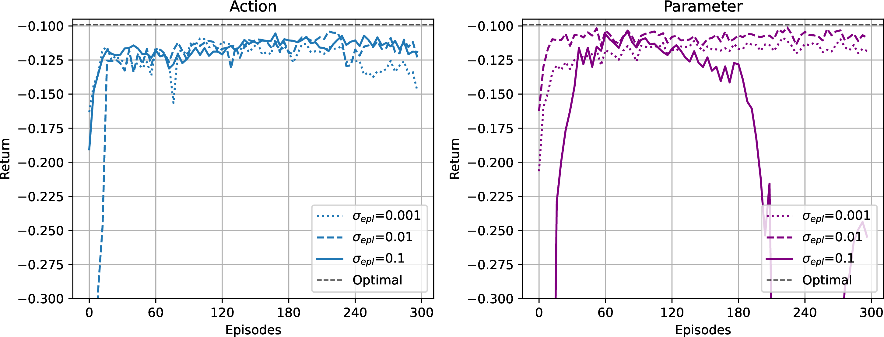
Our experiments suggest that, with appropriate tuning of the perturbation scale in Approach II, the two approaches achieve comparable performance in standard mean field control problems. However, in certain extended MFC problems, the dependence on the control law can make Approach I less effective, resulting in slower convergence. See Section 5.2 for details.

4.2 Implementation details↩︎

4.2.0.1 McKean-Vlasov dynamics simulator.

We construct a black-box simulator of the McKean–Vlasov dynamics (9 ) using a standard particle approximation with Euler–Maruyama discretization [33], and observe the resulting state and control trajectories as well as the associated rewards.

Specifically, let \(h>0\) be the time step size, and \(M\in \mathbb{N}\) be the number of homogeneous agents (particles). Let \((x_{kh,j},a_{kh,j})\) be the state-action of the \(j\)-th agent at time \(kh\), for \(j=1,\ldots, M\), define the empirical measures \(\hat{\mu}_{kh}\mathrel{\vcenter{:}}= \frac{1}{M}\sum_{j=1}^M\delta_{x_{kh,j}}\) and \(\hat{\Gamma}_{kh}\mathrel{\vcenter{:}}=\frac{1}{M}\sum_{j=1}^M\delta_{(x_{kh,j},a_{kh,j})}\), and simulate the states at time \((k+1)h\) by \[x_{(k+1)h,j}\mathrel{\vcenter{:}}= x_{kh,j}+ b(kh,x_{kh,j},a_{kh,j},\hat{\Gamma}_{kh})h+\sigma(kh,x_{kh,j},a_{kh,j},\hat{\Gamma}_{kh})\sqrt{h} Z_{kh,j},\quad 1\leq j\leq M,\] where \(\{Z_{kh,j} \}_{ k=0,\ldots, \lceil T/h\rceil, j=1,\ldots, M}\) are independent \(m\)-dimensional standard normal random vectors. The observed instantaneous reward at time \(kh\) is given by \(r_{kh,j}=r(kh,x_{kh,j},a_{kh,j},\hat{\Gamma}_{kh})\), and the reward at time \(T\) is given by \(r_{T,j}=g(x_{T,j},\hat{\mu}_{T})\), for all \(j=1,\ldots, M\).

4.2.0.2 Critic update.

Due to the off-policy nature of Algorithm 1, we store the observed transition \(\big(kh,x_{kh,j},a_{kh,j},r_{kh,j}, x_{(k+1)h,j}\big)_{j=1}^M\) in a replay buffer \(\mathcal{R}\), and re-sample them later to update actor and critic. We also store the terminal state and reward \((Kh,x_{Kh,j},r_{Kh,j})_{j=1}^M\) in \(\mathcal{R}\). For brevity, we denote by \(\tilde{x}_t\) the concatenation of time and state \((t,x_t)\). We also employ a target value network \(V_{\phi^{tgt}}\), whose parameters are updated as an exponential moving average of the value network parameters. This technique is widely used in modern deep RL algorithms, including DDPG [34] and SAC [35], to improve training stability.

During each episode, after every \(m\geq 1\) steps of simulation, we sample a batch of transitions \(\{\mathcal{D}^{(i)}\}_{i=1}^B\) from replay buffer \(\mathcal{R}\) where \(\mathcal{D}^{(i)}=\big(\tilde{x}^{(i)}_{k_ih,j}, a^{(i)}_{k_ih,j}, r^{(i)}_{k_ih,j},\tilde{x}^{(i)}_{(k_i+1)h,j}\big)_{j=1}^M\), corresponding to different trajectories and time indices, and define the martingale loss by \[\begin{align} \label{eq:martingale95loss} \begin{aligned} &\mathcal{L}^{\mathcal{M}} \mathrel{\vcenter{:}}=\frac{1}{BM}\sum_{i=1}^B\sum_{j=1}^M \Big(V_\phi(\tilde{x}^{(i)}_{k_ih,j},\hat{\mu}^{(i)}_{k_ih})-[r^{(i)}_{k_ih,j}-q_\psi(\tilde{x}^{(i)}_{k_ih,j},a^{(i)}_{k_ih,j},\hat{\Gamma}^{(i)}_{k_ih})]h-e^{-\beta h}V_{\phi^{tgt}}(\tilde{x}^{(i)}_{(k_i+1)h,j},\hat{\mu}^{(i)}_{(k_i+1)h})\Big)^2, \end{aligned} \end{align}\tag{30}\] where \(q_\psi\) is given by (29 ). Note that \(\partial_\phi\mathcal{L}^\mathcal{M}\) and \(\partial_\psi\mathcal{L}^\mathcal{M}\) are stochastic estimates of the semi-gradients in (27 ) and (28 ), respectively. To enforce the terminal constraints, we also sample a batch of terminal states \(\{\mathcal{D}_{ter}^{(i)}\}_{i=1}^B\) from \(\mathcal{R}\) from different trajectories and compute the terminal loss \[\label{eq:terminal95loss} \mathcal{L}^\mathcal{T}=\frac{1}{BM}\sum_{i=1}^B\sum_{j=1}^M(V_\phi(\tilde{x}^{(i)}_{Kh,j},\hat{\mu}^{(i)}_{Kh})-r^{(i)}_{Kh,j})^2.\tag{31}\] The losses \(\mathcal{L}^\mathcal{M}\) and \(\mathcal{L}^\mathcal{T}\) are combined to update the critics \(V_\phi\) and \(q_\psi\) via gradient descent.

4.2.0.3 Actor update.

To implement the exact policy gradient of the current policy \(\varphi_\theta\) given in (?? ), we sample a batch \(\{\mathcal{D}^{(i)}\}_{i=1}^B\) from \(\mathcal{R}\), and define the actor objective by \[\label{eq:policy95loss} \mathcal{L}^\mathcal{A}=\frac{1}{MB}\sum_{j=1}^M\sum_{i=1}^B q_\psi\big(\tilde{x}_{k_ih,j},\varphi_\theta(\tilde{x}_{k_ih,j},\hat{\mu}_{k_ih}),\Gamma^\theta_{k_ih}\big)h,\quad \Gamma^\theta_{k_ih}\mathrel{\vcenter{:}}=\frac{1}{M}\sum_{j=1}^M\delta_{(x_{k_ih,j},\varphi_\theta(\tilde{x}_{k_ih,j},\mu_{k_ih}))}.\tag{32}\] Note that \(\partial_\theta\mathcal{L}^\mathcal{A}\) is a stochastic estimator of policy gradient (?? ).

4.2.0.4 Full algorithm.

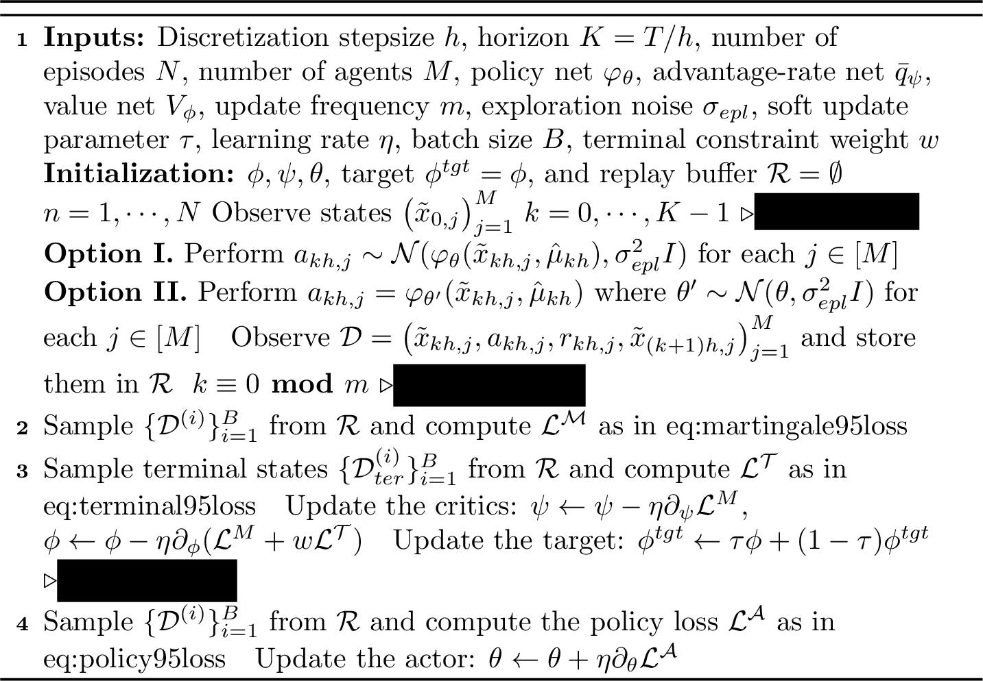
The full procedure of Continuous Time Deep Deterministic Policy Gradient (CT-DDPG) for extended MFC problems is summarized in Algorithm 1.

5 Numerical Experiments↩︎

In this section, we illustrate the efficiency of the proposed CT-DDPG algorithm within the general learning MFC framework. Unless otherwise specified, CT-DDPG refers to the implementation with action space exploration (Option I in Algorithm 1).

5.1 Consensus control of Cucker-Smale model↩︎

We consider the consensus control of multi-dimensional stochastic Cucker-Smale (C-S) models studied in [36], [37]. In this problem, the agent aims to enforce consensus emergence of an interactive particle system via external intervention.

Let \(T>0\), and consider the following \(2n\)-dimensional controlled McKean-Vlasov dynamics, which can be viewed as the large population limit of the finite-particle model studied in [38]: for all \(t\in [0,T]\), \[\label{eq:cs95model} {\mathrm{d}}z_t=v_t{\mathrm{d}}t,\qquad {\mathrm{d}}v_t=\left(\alpha_t+\int_{{\mathbb{R}}^n\times {\mathbb{R}}^n} \kappa(z_t,v_t,z',v')\mathbb{P}_{(z_t,v_t)}({\mathrm{d}}z',{\mathrm{d}}v')\right){\mathrm{d}}t+\sigma{\mathrm{d}}W_t,\tag{33}\] with an initial state \((z_0,v_0)\in L^2(\mathcal{F}_0;{\mathbb{R}}^n\times {\mathbb{R}}^n)\), where \(\sigma\in\mathbb{R}^{n\times n}\), \(W\) is an \(n\)-dimensional Brownian motion, and the interaction kernel \(\kappa:\mathbb{R}^n\times\mathbb{R}^n\times\mathbb{R}^n\times \mathbb{R}^n\to \mathbb{R}^n\) is defined by \[\kappa(z,v,z',v')=\frac{C(v'-v)}{(1+\|z'-z\|^2)^\gamma},\quad \;\text{with some }C,\gamma\geq 0.\] The variables \(z\) and \(v\) represent the position and velocity of a representative particle, respectively. The dynamics (33 ) models the self-organization behavior of a crowd, where the interaction kernel \(\kappa\) captures the decay of influence between agents as their distance increases. It is known that, in the absence of external control, flocking behavior, namely, the convergence of the velocity trajectories \(v\) to a common limit as \(t\to \infty\), occurs only when the parameter \(\gamma\) is sufficiently small.

The aim of the agent is to either induce consensus on models that would otherwise diverge, or to accelerate the self-organization behavior. Specifically, given \(c>0\), we consider maximizing the following reward functional over all adapted controls \(\alpha\): \[J(\alpha) = -\mathbb{E}\left[\int_0^T ( |v_t-\mathbb{E}[v_t] |^2+c |\alpha_t |^2){\mathrm{d}}t + |v_T-\mathbb{E}[v_T] |^2\right]\] Note that in the special case with \(\gamma=0\), it is a linear-quadratic (LQ) mean field control problem. In this case, the optimal policy is linear and given explicitly by (see e.g., [39]): \[\label{eq:CS95LQ} \varphi^*(t,z,v,\mu)=-\frac{P(t)}{c}(v-\mathbb{E}_{v'\sim\mu}[v']),\tag{34}\] where \(\frac{{\mathrm{d}}}{{\mathrm{d}}t}P(t)-\frac{1}{c}P(t)^2-2CP(t)+1=0\) with \(P(T)=1\).

5.1.0.1 Baselines.

We compare our CT-DDPG with existing mean-field RL algorithms, including Actor-Critic (AC) [19], which requires the action dependence of dynamics to be explicitly known, and q-Learning [14], which relies on a closed-form policy given by state-dependent Gibbs measures. Due to the model-aware nature of these two methods, and especially their incompatibility with deep RL framework, we evaluate them only in the LQ case. In addition to the default procedures described in Algorithm 1, we also consider a variant CT-DDPG-Flow, which learns the value function \(\hat{V}\) directly based on the deterministic flow characterization in Theorem 4, while still using the decoupled advantage rate estimator \(\hat{q}_D\) to represent \(\hat{q}\).

5.1.0.2 Model architecture.

Across all experiments, the policy, advantage network, and value network in CT-DDPG and its variants are implemented as three-layer fully connected MLPs with ReLU activations and hidden width \(400\). To incorporate temporal information, we augment the environment observations with a sinusoidal embedding, yielding \(\tilde{x}_t=(\cos(\tfrac{2\pi t}{T}),\sin(\tfrac{2\pi t}{T}),z_t,v_t)\), where \(T\) denotes the maximum horizon. To embed the mean-field distribution, the default parameterization of CT-DDPG is given by \[\label{eq:value95param} V_\phi(\tilde{x}_t,\mu_t)=NN_{\phi_1}\left(\tilde{x}_t,\mathbb{E}_{x'\sim\mu_t}NN_{\phi_2}(x')\right), \tag{35}\] where \(\phi=(\phi_1,\phi_2)\) and similarly for \(\varphi_\theta\) and \(\bar{q}_\psi\). Here we use a learnable feature map to preserve the model-agnostic nature of our method. We also consider a variant based on prescribed moment features of the distribution, referred to as CT-DDPG-Moment: \[\label{eq:value95param95moment} V_\phi(\tilde{x}_t,\mu_t)=NN_\phi\left(\tilde{x}_t,\mathbb{E}_{x'\sim\mu_t}[x'],\mathrm{Var}_{x'\sim\mu_t}[x']\right), \tag{36}\] As a benchmark, we further evaluate a variant that incorporates prior knowledge of the dynamics through a hand-crafted feature map, which we denote by CT-DDPG-Kernel: \[\label{eq:value95param95kernel} V_\phi(\tilde{x}_t,\mu_t)=NN_\phi\left(\tilde{x}_t,\mathbb{E}_{(z',v')\sim\mu_t}\left[\frac{v'-v_t}{(1+\|z'-z_t\|^2)^\gamma}\right]\right), \tag{37}\] This variant requires the exponent \(\gamma\) to be specified a priori, and is therefore less model-agnostic than the default parameterization. Nevertheless, all these variants remain model-free in the sense that they do not exploit closed-form expressions for the optimal policy or value function, in contrast to previous works such as [14], [19].

For AC and q-Learning, we follow [14], [19] respectively and adopt the model-aware LQ parameterization. Specifically, the value function is parameterized as a quadratic function of the state and the policy as a linear function of the state with time dependence incorporated through a three-layer MLP based embedding.

5.1.0.3 Training hyperparameters.

We set dimension \(n=3\) and simulate \(M=50\) homogeneous agents to approximate the McKean-Vlasov dynamics. To accelerate training, we run 8 environments in parallel, i.e., collecting 8 trajectories per episode. All neural networks are optimized by Adam with a learning rate of \(3\times 10^{-4}\) and a batch size of \(B=256\). The update frequency is \(m=1\). The soft target update parameter is \(\tau=0.1\). The weight for the terminal value constraint is \(w=0.002\). And the default exploration noise scale is \(\sigma_{\text{epl}}=0.1\). The entropy regularization coefficient in AC and q-Learning is \(0.01\).

5.1.0.4 Results for LQ case.

We first set \(\gamma=0,C=1,c=0.1,\sigma=0.3,T=1\) in C-S dynamics and the initial state distribution is \(\mu_0=\text{Unif}([0,1]^n)\times\text{Unif}([-1,1]^n)\). The optimal policy is given explicitly in (34 ). We shall examine the effect of different discretization step sizes; the corresponding results are reported in 2.

Observe that CT-DDPG achieves the fastest convergence to the optimal value, despite not explicitly exploiting the LQ structure. In contrast, AC and q-Learning adopt an LQ-based parameterization and nevertheless underperform CT-DDPG, further demonstrating the effectiveness of the proposed method.

5.1.0.5 Results for non-LQ case.

We further set \(\gamma=1\), which imposes a non-trivial coupling between \(z\) and \(v\). The results of different distribution embedding methods in CT-DDPG are shown in 3. We observe that both CT-DDPG and CT-DDPG-Kernel converge rapidly, indicating that a learnable neural network feature map can achieve performance comparable to that obtained when prior information is incorporated. This demonstrates the efficiency and robustness of the proposed approach, as well as its compatibility with the deep RL framework. Although CT-DDPG-Moment uses only generic moment embeddings of the distribution and therefore converges more slowly, it still eventually attains the same optimal return as CT-DDPG. This further illustrates the effectiveness of deep-RL-based methods for MFC problems. For CT-DDPG-Flow, it converges rather slowly, and the performance gap becomes more pronounced as \(h\) decreases. As discussed in 4, although the value function can be directly characterized via Theorem 4, the martingale-based temporal difference loss induced by Theorem 5 provides a more informative signal for learning the decoupled value function, thereby substantially accelerating convergence.

To compare different exploration strategies, we evaluate CT-DDPG with both action-space and parameter-space exploration under varying exploration noise scales. As shown in 4, action-space exploration is more robust to the choice of noise scale, both in terms of convergence rate and final performance. In contrast, parameter-space exploration may suffer from severe instability when the perturbation scale is not properly tuned. Overall, with appropriate tuning, the two approaches achieve comparable performance in standard MFC problems.

5.2 Optimal liquidation with trade crowding↩︎

In this section, we examine the performance of Algorithm 1 in a portfolio liquidation problem with trading crowd, as studied in [1], [23], [33]. In this problem, a large number of market participants aim to liquidate their positions in the same asset by a fixed terminal time \(T\), while accounting for the permanent price impact induced by their trading actions. The resulting cooperative equilibrium gives rise to an extended MFC problem for a representative agent.

Let \((\alpha_t)_{t\in [0,T]}\) denote the trading speed chosen by the representative agent. The state dynamics of the extended MFC problem are given by: for all \(t\in [0,T]\), \[\label{eq:liquidation} {\mathrm{d}}Q_t = \alpha_t {\mathrm{d}}t, \quad {\mathrm{d}}S_t = \lambda \mathbb{E}[\alpha_t]{\mathrm{d}}t + \sigma{\mathrm{d}}W_t.\tag{38}\] Here \(Q=(Q_t)_{t\in [0,T]}\) denotes the inventory process with a random initial state \(Q_0\) representing the initial inventories for all participants, \(S=(S_t)_{t\in [0,T]}\) is the asset price process, the term \(\lambda {\mathbb{E}}[\alpha_t]\) with \(\lambda \ge 0\) captures the permanent market impact on the asset price induced by the aggregate trading of all participants, and \(W\) is a one-dimensional Brownian motion representing exogenous market noise. The objective of the agent is to maximize the following reward functional over all adapted trading speeds: \[\label{eq:liquidation95reward} J (\alpha)= \mathbb{E}\left[\int_0^T -(Q_t^2+\alpha_tS_t+c \alpha_t^2){\mathrm{d}}t + Q_T(S_T-CQ_T)\right],\tag{39}\] where the term \(\alpha_t(S_t+c\alpha_t)\) represents the instantaneous liquidation cost with \(c>0\) representing the linear temporary market impact, \(Q^2_t\) penalizes inventory risk over time, and \(Q_T(S_T-CQ_T)\) with \(C>0\) is the liquidation value of the remaining inventory at terminal time.

Note that (38 ) and (39 ) constitute an LQ extended MFC problem and the optimal policy is given by (see e.g., [39]): \[\varphi^*(t,s,q,\mu)=-\frac{1}{c}\left(P_C(t)(q-\mathbb{E}_{q'\sim\mu}[q'])+P_{C-\frac{\lambda}{2}}(t)\mathbb{E}_{q'\sim\mu}[q']\right),\] where for all \(r\in\mathbb{R}\), \((P_r(t))_{t\in [0,T]}\) satisfies \(\frac{{\mathrm{d}}}{{\mathrm{d}}t}P_r(t)-\frac{1}{c}{P_r(t)}^2+1=0\) with \(P_r(T)=r\). The model architectures and training hyperparameters are the same as described in the previous section. We set \(\lambda=0.2, \sigma=0.3,c=0.1, C=1,T=1, h=0.0005\) and the initial mean-field distribution is \(\mu_0=\text{Unif}([0.8,1.2])\times\text{Unif}([0.8,1.2])\).

The results of CT-DDPG with different exploration mechanisms are shown in 5. Action-space exploration converges rapidly and robustly to the optimal value under various exploration noise scales, demonstrating its effectiveness for the extended MFC problems. Parameter-space exploration is still sensitive to noise scale, but it exhibits a faster convergence if the noise scale is properly tuned. Due to the specific structure of the liquidation problem, action space exploration does not change the expected control, and therefore provides limited exploration for the price process in (38 ), leading to slightly slower convergence. This illustrates the potential advantage of parameter-space exploration in certain extended MFC problems, provided that the hyperparameters are chosen appropriately.

In summary, CT-DDPG exhibits superior performance in terms of convergence speed and stability across all environment settings, verifying the efficiency and robustness of our method.

6 Proofs↩︎

6.1 Proofs of Technical Results↩︎

This section establishes several technical results used in the proofs of Theorems 1 and 3.

We first recall that when the function \(V(\cdot, \cdot,\theta)\) defined in (3 ) is in \(C^{1,2 }([0, T] \times \mathcal{P}_2(\mathbb{R}^n))\), it is the unique solution to an associated linear PDE.

Using Lemma 1, the following proposition characterizes the performance difference between two value functions \(V(\cdot, \cdot,\theta)\) and \(V(\cdot,\cdot,{\theta'})\). It extends the performance-difference lemmas in [4] and [21] from classical control problems to the more general setting of McKean–Vlasov dynamics.

We further prove the joint continuity of the state law with respect to time and the parameter.

6.2 Proofs of Theorems 1, 2, 3 and 5↩︎

We now prove Theorem 1 based on Proposition 6 and Lemma 2.

We further prove Theorems 2 and 3.

Acknowledgements and Disclosure of Funding

Huyên Pham is supported by the Société Générale Chair “Risques Financiers", FiME (Laboratory of Finance and Energy Markets), and the EDF–CACIB Chair”Finance and Sustainable Development”. Yufei Zhang’s research is supported by CNRS-Imperial “Abraham de Moivre” International Research Lab in Mathematics.

References↩︎