1 Introduction↩︎

Many sequential decision-making problems require a learner to repeatedly select actions from a continuous domain in response to an environment whose feedback is evolving over time. A natural and recurring structure in such settings is piecewise-continuous feedback: the reward function is piecewise-Lipschitz within regions of the action space, but changes abruptly across region boundaries. This structure arises organically in a broad range of applications — in principal-agent settings such as dynamic pricing [1], [2] and contract design [3], where the agent’s best response to the learner’s action creates sharp discontinuities in the reward function, and in algorithm configuration and parameter tuning [4]–[7], where an algorithm’s overall performance over instances as a function of its parameters is naturally piecewise-continuous.

Underlying all of these settings is a common computational primitive: proportional sampling from a dynamically evolving weight function. At each round, the learner must select an action with probability proportional to the cumulative rewards observed so far — a distribution that changes as new feedback arrives and the partition of the domain is refined. Proportional sampling is well-studied in static settings [8]–[10], and plays a central role in randomized algorithms [11], online learning [12], and importance sampling. However, the dynamic setting we consider is fundamentally different: each round introduces a new piecewise-structured update to the weight function, and as these updates accumulate over \(t\) rounds in a \(d\)-dimensional domain, the number of distinct regions induced by the partition grows as \(O(t^d)\). This combinatorial explosion makes naively maintaining the weight function and sampling from it computationally infeasible — and yet, to our knowledge, the question of how to do this efficiently has received almost no attention. Prior work on online learning with piecewise-structured rewards [4] has focused primarily on regret minimization and sample complexity, either assuming access to a sampling oracle or ignoring computational efficiency altogether. The only related result is due to [13], who give an efficient algorithm for the one-dimensional piecewise-constant case—a special case of our setting. We address this gap directly.

We study the following online setting. At each round \(t \in \{1, \ldots, T\}\), an adversary introduces a partition of a \(d\)-dimensional domain \([0,1]^d\) into regions, each assigned a structured reward function. The cumulative reward function \(H_t(x)\) accumulates these rewards over time, and the learner’s goal at each round is to sample an action \(x_t\) proportionally to a function of \(H_t(x)\). The reward functions we consider are piecewise-polynomial with partition boundaries defined by hyperplanes from a fixed set of directions, e.g., axis-parallel hyperplanes. The key difficulty is that as partitions accumulate over \(t\) rounds in \(d\) dimensions, the number of distinct regions grows as \(O(t^d)\), and the learner must sample from the induced distribution in real time without explicitly enumerating all regions.

The central computational challenge is maintaining a representation of \(H_t\) that supports efficient sampling as the partition grows. A natural approach is to maintain a data structure that tracks the evolving partition and aggregates rewards across regions. However, this faces two fundamental difficulties. First, each new partition introduced by the adversary interacts with all previous ones: a new hyperplane along one coordinate must be reconciled with all existing boundaries along every other coordinate, triggering a cascade of updates that can touch \(O(t^d)\) regions in a single round. Second, even if one could maintain the partition explicitly, sampling from the induced distribution requires computing region-wise cumulative weights — a task that becomes increasingly expensive as the partition refines. These difficulties compound in high dimensions, and under a fully adversarial environment, such cascades can be forced to occur at every round, making efficient maintenance provably intractable. This motivates a natural restriction on the adversary, which we discuss next.

We resolve the challenges above by providing a \(d\)-dimensional hierarchical data structure that maintains the evolving weight function and supports efficient proportional sampling under a \(\sigma\)-smoothed adversary. We address the potential \(O(t^d)\) cascade triggers per round with two key ideas. First, we introduce a deferred insertion mechanism that avoids propagating each new boundary through all affected regions immediately, instead recording contributions at higher levels of the hierarchy and recovering them efficiently during sampling. Second, we represent cumulative rewards using a parametric vector encoding that allows deferred contributions to be scaled and composed correctly across regions in \(O(1)\) time, even for piecewise-linear and more general polynomial rewards. Together, these ideas reduce the per-round cost from \(O(t^d)\) to a quantity that depends only on the depth of the data structure — which, under \(\sigma\)-smoothness, we show remains sublinear in \(T\). Our main contributions are as follows:

• Efficient hierarchical data structure for proportional sampling. We design a \(d\)-dimensional hierarchical interval-tree data structure that supports efficient updates, cumulative reward queries, and exact proportional sampling under dynamically evolving piecewise-polynomial weight functions. Under a \(\sigma\)-smoothed adaptive adversary, operation runs in \(O(d \cdot t^{\frac{d+1}{2}})\) time per round, and \(O(d \log^{d+1} t)\) under a random-order oblivious adversary. (1)

• Smoothed analysis of tree depth and the longest increasing subsequence problem. We prove a tight \(O(\sqrt{T})\) bound on the depth of our data structure under a \(\sigma\)-smoothed adaptive adversary, and \(O(\log T)\) under a random-order oblivious adversary. To our knowledge, these are the first such results for hierarchical interval-tree structures under smoothed adversaries. Our analysis introduces and optimally solves the expected length of the “longest increasing subsequence under smoothed adversary” problem, which is of independent interest. (2)

• Efficient online learning. We apply our framework to online learning with piecewise-structured rewards, obtaining efficient implementations of the Weighted Majority algorithm under full-information feedback and \(\mathrm{\small EXP3}\) under bandit feedback while satisfying no-regret for piecewise constant and linear settings. ([thm:full-info,thm:bandit])

1.1 Overview of Results and Techniques↩︎

1.1.0.1 Efficient and Scalable Multi-Dimensional Data Structure.

Our framework is built on a hierarchical interval-tree structure with one layer per coordinate. In \(d\) dimensions, the construction is recursive: each node at one level maintains an associated interval tree over the next coordinate, yielding a tree-of-trees representation in which are defined by intersections of intervals across coordinates. In the online proportional sampling setting, successive refinements induce up to \(O(t^d)\) atomic regions by round \(t\), making direct maintenance of the full structure infeasible. We introduce a deferred insertion mechanism, called Lazy Insertion, which avoids cascading each newly introduced boundary through all associated structures as in classical multi-dimensional interval trees [14]. This mechanism is enabled by a novel compact parametric vector representation of rewards, which allows updates and insertions to be handled efficiently while preserving scalable propagation across subregions. We then analyze the height and balance of the resulting data structure under adaptive and oblivious \(\sigma\)-smooth adversaries, and use these bounds to derive the efficiency and regret guarantees in our proportional sampling and online learning applications.

1.1.0.2 Lazy and Regular Associated \(\texttt{Interval Tree}\)s.

Our data structure maintains cumulative weight information over all atomic and non-atomic regions induced by the evolving partition of the space. Concretely, at each level it stores an interval tree over the endpoints obtained by projecting region boundaries onto the corresponding coordinate. In a classical insertion scheme, the endpoints induced by each newly formed region must be propagated into all associated structures corresponding to the relevant subregions, so that every node explicitly reflects the current partition. Our key observation is that, since the data structure is designed to preserve proportional sampling rather than explicitly storing every induced subregion in all levels, many of the classical insertions can be deferred. To achieve this, each node maintains two associated data structures: a regular structure, which is updated as in the classical setting, and a lazy structure, which stores deferred insertions. During an update, newly introduced endpoints are propagated only along the traversal paths needed to locate the affected regions. Whenever the traversal reaches a node whose subtree lies entirely inside the relevant interval, the cascade stops: instead of inserting the remaining endpoints into all descendant associated structures, they are recorded in the lazy structure of that node and later scaled to the underlying subregions during queries. As a result, while classical maintenance may require \(O(t^d)\) insertions per newly induced partition, our lazy mechanism reduces the number of required insertions to \(O\left(\prod_{i\in[d]} \texttt{Height}(\mathcal{T}^{(i)})\right)\), where \(\texttt{Height}(\mathcal{T}^{(i)})\) denotes the expected height of the interval tree at level \(i\), built over the endpoints obtained by projecting boundaries onto the \(i\)-th coordinate. The conceptual idea is illustrated in 3 for the two-dimensional case, which provides useful intuition for the underlying architecture.

This approach differs from classical lazy propagation in one-dimensional dynamic trees [13], [15], where segments are inserted explicitly and only their weight updates are deferred. In contrast, Lazy Insertion defers the insertions themselves, allowing the affected subtrees to remain implicitly represented while preserving correctness.

1.1.0.3 Scalable Cumulative Reward Vectors.

To ensure that the information maintained in the lazy structures remains constantly scalable and can be accurately combined with the regular structures during sampling, we introduce scalable cumulative reward vectors in place of scalar cumulative rewards. For an inserted region, each such vector represents the aggregate reward (integral of the reward function) over that region, with its entries capturing the contributions of the different monomial terms arising in the integration process. Although summing these entries recovers the usual real-valued reward of the region, the vector representation allows each term to be scaled independently through closed-form expressions. This property is essential beyond piecewise-constant rewards, such as for piecewise-linear and more general structured reward functions, where direct scalar scaling is no longer feasible. In turn, this representation enables the lazy insertion structures to scale maintained reward information down to affected subregions in \(O(1)\) time and to compose it correctly with the explicitly maintained regular information, thereby preserving accurate proportional sampling. We illustrate this mechanism further in Example 2 in Section 3.

1.1.0.4 Balanced Interval Trees under \(\sigma\)-Smoothed Adversaries.

Having reduced the insertion cost per region from \(O(t^d)\) to a traversal-depth term, the overall efficiency is governed by the expected height of the interval tree at each level. We therefore analyze this height under \(\sigma\)-smoothed adversaries. We prove an asymptotically tight \(O(\sqrt{\sigma T})\) upper bound under both adaptive and oblivious adversaries. Thus, for the tree growth, adaptivity is no more powerful than obliviousness within the same sample budget. This contrasts with [16], where adaptive adversaries are approximated by oblivious i.i.d.uniform samples using more draws. In our setting, merely the arrival order of the endpoints determines the height, and oblivious sequences already match the adaptive \(O(\sqrt{\sigma T})\) worst case. Under the more restrictive random-order oblivious adversary, the expected height further improves to \(O(\log T)\). This analysis implies efficiency of operations without the need to rebalance the tree.

1.1.0.5 Time Complexity.

Our data structure supports online proportional sampling efficiently, even though the number of atomic regions can grow as \(O(t^d)\) by round \(t\). In particular, any data structure operation including sampling an action at round \(t\) from the current proportional distribution, can be implemented in time \(O\!\left(d \prod_{i=0}^d \texttt{Height}(\mathcal{T}^{(i)}) \right)\), where under an adaptive \(\sigma\)-smoothed adversary this becomes \(O(d\, t^{\frac{d+1}{2}})\), while under an oblivious \(\sigma\)-smoothed adversary it becomes \(O(d \log^{d+1} t)\). The running time captures both the hierarchical traversal of the multi-dimensional interval tree and the lazy insertion mechanism used to maintain scalable cumulative reward information.

1.1.0.6 Data Structure and Efficient Regret Analysis under Full Information and Bandit Feedback.

Our data structure also extends to adversarial online learning under both full-information and bandit feedback. We analyze the regret of the efficient \(\texttt{Weighted Majority}\) and \(\texttt{EXP3}\) algorithm under both full-information and bandit-feedback settings in a \(d\)-dimensional \(\text{action parameter space}\), where the adversary selects piecewise constant or linear reward functions. Our analysis extends the results of [13] and aligns with the framework of [4], demonstrating that the regret remains sublinear in time.

1.1.0.7 Organization.

In 3, we formalize our model of proportional sampling with dynamically evolving, piecewise-continuous weight functions. 4 introduces our framework for an efficient and scalable data structure. 5 presents efficient implementation of our algorithm for proportional sampling. We then extend our framework to online learning in 6, where we describe efficient algorithms for both full-information and bandit feedback settings. 2 provides extensive literature review. [section:quereis,section:correctness,section:generalpar,section:complexity] provide the details of our data structure’s queries, their correctness proofs, and runtime analysis. Finally, [sec:learningapp,app:bandit] describe our online learning algorithms and establish their regret guarantees.

2 Related Work↩︎

Proportional sampling arises across survey sampling, theoretical computer science, and online learning, but has been studied almost exclusively in discrete or geometrically static settings. In statistics, probability proportional to size (PPS) sampling has a long history [8]–[10]; in randomized algorithms and sketching it underlies sublinear methods [11], [17], [18]; and in randomized linear algebra it drives core sampling schemes [19]. Our setting generalizes these to continuous domains with adversarially evolving geometry with piecewise structure, a regime none of these frameworks are designed to handle. Efficient proportional sampling in such setups bridges the gap between theory and application by making these algorithms practical in realistic, evolving environments.

Another important application of proportional sampling is in online learning, where it underlies foundational algorithms such as the exponentially-weighted forecaster (EWF) [12], Follow the Perturbed Leader [20], and EXP3 [21]. The proportional sampling underlying these algorithms typically operates over finite or convex action spaces with scalar-valued feedback. A separate line of work has studied online learning in settings with piecewise structure, particularly in applications such as pricing, contract design, and security games [1], [2], [4], [22]–[25], focusing on regret guarantees and sample complexity under structural assumptions, but without addressing efficient sampling from evolving feedback functions. Across all these settings, proportional sampling is not merely a statistical tool but a computational primitive whose efficiency in highly evolving, piecewise structured domains determines the practicality of these algorithms, and bridging this gap between theory and application is the central challenge our work addresses.

To support efficient proportional sampling in such settings, we build on and extend the classical data structure literature. Classical data structures such as balanced binary trees, range trees, and quad-trees provide efficient support for operations over structured domains and spatial decompositions [14], [26]. These structures are well-suited to settings where the underlying partition is fixed and aggregates are scalar-valued—supporting value updates over predetermined subregions but not structural change. In contrast, our setting couples dynamic geometric refinement with vector-valued maintenance and continuous sampling: adversarially chosen hyperplanes arrive over time, progressively refining the partition and restructuring which subregions exist. We maintain vector-valued statistics that allow information about each region to be efficiently scaled down to newly created subregions, enabling tractable maintenance as the geometry evolves, and support proportional sampling from distributions defined by cumulative, piecewise polynomial functions.

Designing data structures for online learning has also been studied in the context of fixed hierarchical partitions [27], [28], where chaining and recursive partitioning of the context space are used to construct structured sets of experts and obtain improved regret bounds, with a focus on controlling the complexity of the expert class. Our setting differs fundamentally: the partition is not fixed but evolves as adversarially chosen piecewise-structured rewards arrive over time, and the central challenge is maintaining efficient proportional sampling over this dynamic geometry rather than controlling expert class complexity. Our framework yields regret guarantees under both full-information and bandit feedback, but its primary contribution is the design of scalable sampling mechanisms that make these guarantees achievable in practice.

Our work connects to the smoothed analysis framework [7], [29], which provides the necessary conditions under which learning remains tractable despite discontinuities. The most directly related work is due to [13], who proposed an efficient algorithm for one-dimensional learning with fixed, piecewise-constant feedback against a \(\sigma\)-smoothed adversary; we build on and significantly generalize their framework to accommodate high-dimensional domains, dynamically evolving piecewise structure, and more expressive piecewise polynomial functions.

Our analysis of hierarchical interval-tree height under \(\sigma\)-smoothed adversaries is the first of its kind. While prior smoothing results [16] approximate the set of adversarially generated endpoints by i.i.d.samples, they do not capture the order of arrival, which is crucial for tree growth in our setting. This distinction leads to our tight \(O(\sqrt{\sigma T})\) bound under adaptive \(\sigma\)-smoothed adversaries, in contrast to the \(O(\log T)\) behavior that holds under i.i.d.arrivals [30].

Finally, recent work on structured learning in multi-dimensional settings has begun to address computational concerns [24], [31], but falls short of the logarithmic-in-time complexity required for efficient online sampling in dynamic environments. Our work is the first to design a data structure that supports exact proportional sampling over a continuously partitioned domain with time-varying piecewise polynomial rewards, while providing regret guarantees under both full-information and bandit feedback, closing the gap between the theoretical foundations laid by prior work and the computational demands of realistic, evolving environments.

3 Model: Adversarial Online Proportional Sampling↩︎

We consider a proportional sampling problem over the domain \([0,1]^d\), where \(d \in \mathbb{N}\). At each round \(t\), the learner samples a point \(x_t \in [0,1]^d\), while a piecewise-structured reward function \(h_t\) is adversarially defined as follows:

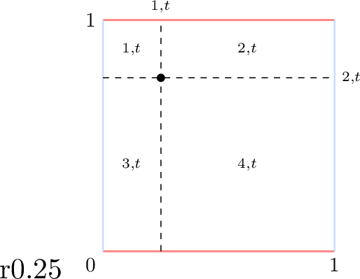
1. Action Space Partitioning: At each round \(t\), the domain \([0,1]^d\) is partitioned, as in Figure 1, into disjoint regions \(\mathcal{P}_t = \{ \rho_{1,t}, \rho_{2,t}, \dots \}\) by a set of \(k \in \mathbb{N}\) hyperplanes \(\Psi_t = \{ \psi_{1,t}, \dots, \psi_{k,t} \}\) chosen by an adversary. Each hyperplane is parallel to some direction \(\gamma_i\) in a fixed set \(\Gamma= \{\gamma_1, \dots, \gamma_m\}\) of pairwise non-parallel reference directions. Under the \(\sigma\)-smooth model, for each direction \(\gamma_i\), hyperplanes parallel to \(\gamma_i\) are drawn independently from an adversarially chosen \(\sigma\)-smooth distribution \(\mathcal{D}^{(i)}_t\) over \([0,1]\), with independence across directions, where a distribution is \(\sigma\)-smooth if its probability density function is bounded above by \(\sigma \geq 1\). Smoothness is imposed separately within each directional group.

2. Reward Assignment: A piecewise-structured reward function \(h_t : [0,1]^d \to \mathbb{R}_{\geq 0}\) is assigned over the partition \(\mathcal{P}_t\). Specifically, each region \(\rho_{j,t} \in \mathcal{P}_t\) is associated with a non-negative reward function \(h_{j,t}\), and \(h_t(x)=h_{j,t}(x)\) for all \(x \in \rho_{j,t}\). We assume that all region-wise reward functions share a common functional form (e.g., a fixed polynomial), while their parameters—namely, the coefficients of the corresponding monomials—may vary across regions and rounds. Thus, the reward function differs across regions only through its parameters, not its structure. We define the cumulative reward function as \[H_t(x)\doteq\sum_{t'=1}^t h_{t'}(x).\]

We study the problem of efficiently sampling \(x_t\) from a distribution proportional to a transformation \(\zeta: \mathbb{R} \to \mathbb{R}_{\geq 0}\) of the cumulative reward: \[\begin{align} x_t \sim \frac{\zeta\!\left(H_t(x)\right)}{\int_{x \in [0,1]^d} \zeta\!\left(H_t(x)\right)}. \label{eq:proportional} \end{align}\tag{1}\] Two canonical choices of \(\zeta\) recover standard sampling schemes: When \(\zeta(H_t(x))=H_t(x)\), this reduces to proportional sampling, i.e., \(x_t \sim \frac{H_t(x)}{\int_{x \in [0,1]^d} H_t(x)}.\) When \(\zeta(H_t(x))=\exp(\eta H_t(x))\) for \(\eta \in (0,1)\), we obtain exponential-weighted sampling: \(x_t \sim \frac{\exp(\eta H_t(x))}{\int_{x \in [0,1]^d} \exp(\eta H_t(x))}.\) The first case naturally extends to polynomial choices of \(\zeta\), while the second case connects this sampling framework to exponential-weight methods in adversarial online learning.

3.0.0.1 Smoothed Adversarial Models.

The sequence of partitions is governed by the hyperplanes \(\{\Psi_t\}_{t\ge1}\). At round \(t\), the adversary selects distributions \(\mathcal{D}^{(\cdot)}_t\) corresponding to directions \(\Gamma\), where the hyperplanes in \(\Psi_t\) are sampled from. The adversary is adaptive if the selection of the distribution depends on previously sampled hyperplanes, based on the past hyperplane sets \(\Psi_1,\dots,\Psi_{t-1}\), and oblivious if the selection is fixed a priori. We also consider random-order oblivious, in which the adversary first selects \(Tk\) distributions, and the sampled hyperplanes arrive in a uniformly random order.

4 Our Framework: Efficient and Scalable Data Structure \(\mathcal{T}\)↩︎

We now introduce our approach for designing a new multi-dimensional data structure that enables efficient proportional sampling and further supports online learning against a \(\sigma\)-smoothed adversary.

4.1 Reward Function Parametric Representation.↩︎

As discussed in the introduction, supporting efficient operations in this rapidly evolving partition requires handling both deferred insertions and downward-scalable auxiliary structures that remain consistent with regular insertions. We capture this through a novel parametric representation of the reward. Rather than storing rewards directly, we assign each region \(\rho_{i,t} \in \mathcal{P}_t\) a coefficient vector in a fixed reward family, from which the reward is recovered via a known mapping. We establish additivity of these vectors across rounds, updates of the form \(H_t = H_{t-1} + h_t\) reduce to simple vector additions. This yields efficient maintenance of cumulative rewards while preserving consistency across regular and deferred operations.

We reinterpret the piecewise reward function \(h_t\), assumed to be piecewise polynomial, as a composition of two components: a mapping function \(g\) and a parameter function \(f_t\). We model the piecewise polynomial reward function \(h_t\) as \(h_t(x)=g(x,f_t(x))\), where: \(g:\mathbb{R}^d\times\mathbb{R}^{n}\to\mathbb{R}\) is a known mapping that specifies a fixed family of log-concave polynomial rewards through a fixed set of \(n\) monomials in \(x\), and \(f_t:\mathcal{P}_t\to\mathbb{R}^{n}\) is a parameter function that assigns to each induced region its coefficient vector.

For instance, for \(h_t(x) = 3x^{(0)} + 5x^{(1)}\), the monomial vector is \(\langle x^{(0)}, x^{(1)}\rangle\), \(f_t = \langle 3, 5\rangle\), and \(g(x, f_t(x)) = \langle x^{(0)}, x^{(1)}\rangle \cdot f_t(x)\) recovers \(h_t\). Thus the monomial family is fixed while the adversary controls region-wise coefficients via reward parameter function \(f_t\); examples for higher-degree polynomials are in 1. As formalized in 7, this induces a natural additive structure over time for parameter functions as \[F_t(x) \doteq \sum_{t' \leq t} f_{t'}(x).\]

4.1.0.1 Remark.

In both feedback models, \(g\) is fixed and known; under full information the learner observes \(f_t\) entirely, while under bandit feedback only \(f_t(\rho_{i,t})\) for the region containing \(x_t\) is revealed.

4.1.0.2 Reward Aggregation over Regions.

4.2 Downward Scalability via Vector Encoding of \(r(\rho)\).↩︎

We represent the cumulative reward of a region \(\rho\) as a vector \(\vec{r}(\rho)\), where each entry corresponds to a monomial component of the reward, enabling computation of \(r(\rho')\) for any subregion \(\rho' \subseteq \rho\) by scaling each entry independently using only the boundaries of \(\rho'\) and \(\rho\).

For example, consider a linear reward of the form \(g(x,F_t(x)) = c_1 x^{(0)} + c_2 x^{(1)}.\) For a rectangular region \(\rho= [a_1{:}a_2][b_1{:}b_2]\), the cumulative reward decomposes to the entries of \(\vec{r}(\rho)\) as \[r(\rho) = c_1 \int_{\rho} x^{(0)} + c_2 \int_{\rho} x^{(1)} \xrightarrow{\text{vector representation}} \vec{r}(\rho) = \left\langle c_1 \int_{\rho} x^{(0)},\; c_2 \int_{\rho} x^{(1)} \right\rangle.\] To compute the aggregate reward over a subregion \(\rho'=[a'_1:a'_2][b'_1:b'_2] \subseteq \rho\), each component is scaled independently using closed-form factors that depend only on the endpoints of \(\rho\) and \(\rho'\), and the results are summed as \[r(\rho') = \vec{r}^{(0)}(\rho)\cdot \frac{(a_2'^2 - a_1'^2)(b'_2 - b'_1)}{(a_2^2 - a_1^2)(b_2 - b_1)} + \vec{r}^{(1)}(\rho)\cdot \frac{(a'_2 - a'_1)(b_2'^2 - b_1'^2)}{(a_2 - a_1)(b_2^2 - b_1^2)}.\] We defer the multivariate construction and scaling procedure to any kind of region to 7.1.

4.3 Tree-Based Data Structure \(\mathcal{T}\)↩︎

\(\mathcal{T}\) is a multi-layered tree-of-trees, one layer per coordinate, that maintains cumulative rewards and supports proportional sampling over a \(d\)-dimensional evolving space. We defer implementation details to 5 and focus here on the key primitives. At each round \(t\), \(\mathcal{T}\) supports:

• \(\texttt{Insert}(\rho_{i,t})\): insert region \(\rho_{i,t} \in \mathcal{P}_t\) induced by discontinuities of \(f_t\).

• \(\texttt{Update}(\rho_{i,t})\): update cumulative rewards with \(f_t(\rho_{i,t})\) across all affected and newly created regions.

• \(\texttt{CReward}(\rho, t)\): return aggregate reward \(r(\rho)\) under \(F_t\) for a query region \(\rho\).

• \(\texttt{Draw}(t)\): sample \(x_t \in \text{action parameter space}\) with probability proportional to \(\zeta\!\left(H_t(x)\right)\) at round \(t\).

Proportional Sampling at each round proceeds as follows:

1. Sampling: issue \(\texttt{Draw}(t)\) to \(\mathcal{T}(t{-}1)\) to proportionally sample \(x_t\) w.r.t.cumulative parameters \(F_{t-1}\).

2. Update: upon observing \(f_t\), insert new regions \(\rho_{i,t} \in \mathcal{P}_t\) and update \(\mathcal{T}\) with \(f_t(\rho_{i,t})\).

By the following theorem, the per-round cost of \(\texttt{Draw}(t)\) (similar to other queries in 13.) decomposes recursively across layers, each contributing a factor of \(\texttt{Height}(\mathcal{T}^{(i)})\), as the height of that layer measured as its longest root-to-leaf path, a fundamental concept governing query complexity in tree-based structures, whose efficiency under smoothness in our highly evolving setting is established below.

4.3.0.1 Balancedness of \(\mathcal{T}\) under Smoothness.

A critical bottleneck for efficiency in any tree-based structure is the height: in the worst case, \(\texttt{Height}(\mathcal{T}^{(i)})\) grows as \(O(TK)\), and classical rebalancing is prohibitively expensive in our tree-of-trees design due to \(O(t^d)\) cascading updates. Surprisingly, we show that smoothness alone prevents any adversary from forcing linear height growth, remarkably resolving the need for explicit rebalancing and making \(\mathcal{T}\) provably balanced without it. By the following theorem, we establish tight bounds sublinear in \(T\) independent of the adversary’s adaptivity; detailed discussion and overview of the techniques are presented in 8.1.

We reduce both adversary types to an \(r^*\)-averse adversary (5) maximizing height along a canonical root-to-leaf path, identify a monotone optimal strategy, and prove tight bounds via a dynamic program for the adaptive case and [30] for the random-order case; full proofs in 8.

4.3.0.2 Connection to Longest Increasing Subsequence.

Our analysis reveals a surprising tight connection to the longest increasing subsequence under a smoothed adversary, a natural and previously unstudied problem, for which we establish a tight \(O(\sqrt{\sigma T})\) bound as a byproduct of our techniques.

5 Online Proportional Sampling for \(\zeta(H_t(x)) = g(x,F_t(x))\)↩︎

We now introduce \(\mathcal{T}\), our data structure for online proportional sampling in this case that maintains aggregate reward vectors \(\vec{r}(.)\) over regions in the evolving space, and supports efficient and accurate sampling through deferred insertions and downward-scaling. For concreteness and clarity, we present the main ideas in the two-dimensional axis-parallel setting and defer the remaining technical details, along with the full \(d\)-dimensional generalization, to the appendix.

5.0.0.1 \(2\)-Dimensional Case with Axis-Parallel Hyperplanes.

We consider a two-dimensional action space with axis-parallel hyperplanes, and focus on the case \(k=2\), where at each round \(t\) one hyperplane parallel to each axis arrives: \(\psi_{1,t} = \{x^{(0)} = c^{(0)}_t\}, \; \psi_{2,t} = \{x^{(1)} = c^{(1)}_t\}, \; \text{where } c^{(0)}_t, c^{(1)}_t \sim \mathcal{D}^{(0)}_t,\mathcal{D}^{(1)}_t.\) Crucially, the hyperplanes partition each coordinate into intervals, so every region can be represented via its coordinate-wise projections as the alignment of one horizontal and one vertical interval. For example, \(\rho_{1,t} = [0{:}c^{(0)}_t][c^{(1)}_t{:}1]\) (1).

5.1 Description of the Data Structure \(\mathcal{T}\)↩︎

We now describe the technical core of \(\mathcal{T}\), a two-dimensional interval-tree structure for maintaining \(F_t\). At a high level, \(\mathcal{T}\) is a tree of trees: each level corresponds to one coordinate, with interval trees tracking projections onto that coordinate, where every node represents an interval whose endpoints are determined by its children’s left and rightmost endpoints. Each node points to interval trees over the other coordinate, maintaining the corresponding projections. To support deferred insertions, these projections are organized into regular and lazy insertion trees: projections are inserted regularly when the corresponding region only intersects the node interval, and lazily when it fully contains it. Both tree types share the same structure but are maintained and queried differently, together capturing all regions without overlap.

Here are the components of the data structure in more detail:

1. Top-Level Tree \(\mathcal{T}^{(0)}\) (Horizontal Intervals). As illustrated in 2 (a), the top-level tree organizes the first coordinate of the action space. Its leaves are the atomic horizontal intervals obtained by projecting atomic regions onto this coordinate. Each internal node accordingly represents a horizontal interval as the contiguous union of its children’s intervals, with the root corresponding to the full interval \([0,1]\).

2. Second-Level Trees (Vertical Intervals). As shown in 2 (c), each node \(v_0 \in \mathcal{T}^{(0)}\) is associated with three interval trees over the second coordinate: one regular insertion tree \(\mathcal{T}^{(1)}_{v_0}\) and two lazy insertion trees \(\mathcal{L}^{(1)}_{v_0}\) and \(\mathcal{R}^{(1)}_{v_0}\). These trees have the same structure as the top-level tree, but over intervals induced by projecting regions onto the second coordinate (2 (b)).

   

   Formally, as illustrated in 3, for a region \(\rho=[c^{(0)}_1:c^{(0)}_2][c^{(1)}_1:c^{(1)}_2]\) in \(f_t\), its vertical projection \([c^{(1)}_1:c^{(1)}_2]\) is inserted as follows:

   • Regular \(\mathcal{T}^{(1)}_{v_0}\): if \(\texttt{Int}(v_0)\) intersects but is not strictly contained in \([c^{(0)}_1,c^{(0)}_2]\) (equivalently, contains either \(c^{(0)}_1\) or \(c^{(0)}_2\)), the projection is regularly inserted at \(v_0\) (e.g., \(v_0\) and \(z_0\), but not \(u_0\) in 3);

   • Lazy \(\mathcal{L}^{(1)}_{v_0}\) / \(\mathcal{R}^{(1)}_{v_0}\): if \(\texttt{Int}(\texttt{Left\_child}(v_0))\) or \(\texttt{Int}(\texttt{Right\_child}(v_0))\) is contained in \([c^{(0)}_1:c^{(0)}_2]\), the projection is recorded lazily in the corresponding left or right lazy tree, avoiding insertion into that subtree (e.g., \(v_0\) and \(z_0\) in 3).

   During queries, deferred contributions stored in lazy structures are recovered via scaling. For example, in 3, the vertical interval \([c^{(1)}_1:c^{(1)}_2]\) of the region \(\rho\) is not inserted into \(\mathcal{T}^{(1)}_{u_0}\), \(\mathcal{L}^{(1)}_{u_0}\), or \(\mathcal{R}^{(1)}_{u_0}\). Instead, the information stored in \(\mathcal{L}^{(1)}_{v_0}\) is scaled and applied to regions whose horizontal projections lie within \(\texttt{Int}(u_0)\).

3. Aggregate Reward Vectors. As mentioned, we maintain a reward vector \(\vec{r}(\rho)\) for each region in the sampling structure. These vectors are stored at the nodes of the second-level trees and are indexed by the chain of nodes followed from the top-level tree, where \(v\)-nodes correspond to regular insertions and \(w\)-nodes to lazy insertions (e.g., \(\vec{r}_{v_0,v_1}\) and \(\vec{r}_{v_0,w_1}\) in the 3). This indexing cleanly separates their contributions: regular vectors are applied directly, while lazy ones are recovered via scaling.

   For instance, in two dimensions, a node \(v_0 \in \mathcal{T}^{(0)}\) together with \(v_1 \in \mathcal{T}^{(1)}_{v_0}\) defines a region \(\rho=[\texttt{Int}(v_0)][\texttt{Int}(v_1)]\), and \(\vec{r}_{v_0,v_1}\) stores the reward from regular insertions, which are applied directly and are not scaled to subregions. In contrast, \(\vec{r}_{v_0,w_1}\) corresponds to a lazy insertion and is scalable along the first coordinate. More generally, \(\vec{r}_{v_0,\ldots,w_j,\ldots}\) represents the region \([\texttt{Int}(v_0)]\cdots[\texttt{Int}(w_j)]\cdots\), with a lazy component at level \(j\) is scalable along dimension \(j-1\). This notation extends naturally to higher dimensions.

4. Auxiliary Trees \(\mathcal{E}^{(0)}\) and \(\mathcal{E}^{(1)}\). The auxiliary trees index all horizontal and vertical endpoints introduced by the adversary up to round \(t\). They do not store reward information; they are standard interval trees used only to quickly identify the atomic regions needed by the drawing procedure.

5.2 Query Handling, Structural Properties, and Time Complexity↩︎

To obtain the efficiency and correctness of \(\mathcal{T}\), matching the \(\mathbb{E}\!\left[\prod_{i\in[d]}\texttt{Height}(\mathcal{T}^{(i)})\right]\) complexity of 1, all query handling is built on two primitives applied recursively along each coordinate over the projection of regions onto that coordinate. For a region \(\rho\) with \([c^{(i)}_1:c^{(i)}_2]\) as its projection along coordinate \(i\) onto a given level-\(i\) interval tree (either lazy or regular), the primitives are:

• Locate leaves \(l_i\) and \(u_i\) as atomic intervals with \(c^{(i)}_1, c^{(i)}_2 \in \texttt{Int}(l_i), \texttt{Int}(u_i)\).

• Traverse from \(l_i\) and \(u_i\) upward along paths \(p_{l_i}\) and \(p_{u_i}\), meeting at the first common ancestor \(v_{l_i,u_i}\).

5.2.0.1 Handling \(\texttt{Insert}(\rho)\) and \(\texttt{Update}(\rho)\).

Both queries proceed by recursively applying locate-and-traverse across all layers of \(\mathcal{T}\). At each level, the paths \(p_{l_i}\) and \(p_{u_i}\) determine which next-level structures receive the projection: regular insertions on \(p_{l_i}\cup p_{u_i}\), and lazy insertions before the paths merge, right-lazy on \(p_{l_i}\setminus p_{u_i}\) and left-lazy on \(p_{u_i}\setminus p_{l_i}\). While insertion decides regular or lazy placement, the update step ensures arithmetic soundness of the cumulative reward vectors: regular updates integrate over \(\rho'\), a subregion whose \(i-1\)-th projection intersects that of \(\rho\), while lazy updates apply over \(\rho''\), a subregion whose \(i-1\)-th projection is uniformly covered by that of \(\rho\), preserving downward scalability. In two dimensions these take the form \[\vec{r}_{v_0,v_1} \gets \vec{r}_{v_0,v_1} + \vec{A}_{\rho'}, \qquad \vec{r}_{v_0,w_1} \gets \vec{r}_{v_0,w_1} + \vec{A}_{\rho''},\] where \(\rho' = [\texttt{Int}(v_0)\cap[c^{(0)}_1,c^{(0)}_2]][.]\) and \(\rho'' = [\texttt{Int}(v_0)][.]\), with \(\vec{A}_{\rho'}\) and \(\vec{A}_{\rho''}\) computed as the vectorized aggregate reward via ?? with \(f_t(\rho)\) as the coefficient vector.

5.2.0.2 Handling \(\texttt{Draw}(t)\).

Has two sampling stages:

(i) atomic region \(\rho\sim\dfrac{\int_{x \in \rho} g(x, F_t(x))dx}{\int_{x' \in [0,1]^d} g(x', F_t(x'))dx}\), (ii) sample \(x_t \sim\dfrac{g(x_t, F_t(x_t))dx}{\int_{x \in \rho} g(x, F_t(x))dx}\) within \(\rho\).

5.2.0.3 Stage 1: Atomic region sampling.

An atomic region is sampled by sequentially selecting an atomic interval along each of the \(d\) coordinates via root-to-leaf traversals of \(\mathcal{E}^{(0)}, \dots, \mathcal{E}^{(d-1)}\), with left/right moves at each node taken with probability computed by \(\texttt{CReward}(\cdot)\) conditioned on intervals fixed along prior coordinates. In two dimensions, horizontal sampling traverses \(\mathcal{E}^{(0)}\) to select \(\texttt{Int}(v_0)\), followed by vertical sampling of \(\mathcal{E}^{(1)}\) conditioned on \(\texttt{Int}(v_0)\), together forming atomic region \([\texttt{Int}(v_0)][\texttt{Int}(v_1)]\) proportionally to \(r([\texttt{Int}(v_0)][\texttt{Int}(v_1)])\). Computing \(\texttt{CReward}(\cdot)\) is highly non-trivial: it constructs set of interval trees \(\mathcal{S}^{(1)}_{v_0}\) via recursive locate-and-traverse by gathering \(\mathcal{T}^{(1)}_{v_0}\) with \(\mathcal{L}^{(1)}_{v_0'}\) or \(\mathcal{R}^{(1)}_{v_0'}\) for each \(v_0' \in p_{v_0}\) and scaling lazy contributions, since atomic endpoints are distributed across structures in \(\mathcal{S}^{(1)}_{v_0}\) and require boundary marginal pruning at each; completeness, endpoint-uniqueness, and downward scalability of lazy reward vectors together ensure correct aggregation without double-counting.

5.2.0.4 Stage 2: Sampling within \(\rho\).

Given the sampled atomic region \(\rho\), we sample \(x_t \in \rho\) proportionally to \(g(x, F_t(x))\) via uniform sampling for piecewise-constant rewards, and Hit-and-Run (7) for more complex piecewise log-concave rewards such as high-degree polynomial and \(\exp\) function.

6 Efficient Adversarial Online Learning \(\zeta(H_t(x)) = \exp(\eta g(x,F_t(x)))\)↩︎

We now show how \(\mathcal{T}\) serves as the computational backbone for \(\texttt{Weighted Majority}\) and \(\texttt{EXP3}\) (22 and [alg:band]), adapting our data structure to support efficient per-round sampling under \(\zeta(x) = \exp(\eta x)\) in our highly evolving setting. At each round \(t\), the adversary selects hyperplanes \(\Psi_t\) and defines a piecewise-structured reward \(h_t\) over the induced partition \(\mathcal{P}_t\) of \([0,1]^d\), and the regret of policy \(\pi\) is \(\operatorname{Regret}(\pi, T) \doteq \max_{x \in [0,1]^d} \sum_{t=1}^T h_t(x) - \mathop{\mathrm{\mathbb{E}}}[\sum_{t=1}^T h_t(x_t)].\) ()

We consider full-information and bandit feedback, focusing on piecewise-constant and piecewise-linear rewards \(h_t\) respectively—a scope dictated by the non-additivity of exponentially weighted cumulative rewards under \(\zeta(x)=\exp(\eta x)\), which breaks the lazy scaling mechanism and renders both exact integration and regret bounding intractable beyond degree one. Each feedback model therefore requires a tailored set of assumptions:

• Full-information: piecewise-constant rewards; adversary \(\sigma\)-smoothed along one direction,

• Bandit: piecewise-linear rewards; general \(\sigma\)-smoothed adversary of 3

The following theorem reflects the implication of \(\mathcal{T}\) for online learning under full-information feedback, where the setup restriction stems from the computational inefficiency of scaling arising from the arithmetic challenges of handling \(\zeta(x) = \exp(\eta x)\) (reflected in Example 3); the full setup, challenges, and proof are presented in 15.

Since new endpoints arrive only along \(\gamma_1\), the height of \(\mathcal{T}^{(0)}\) follows 2, giving \(O(\sqrt{\sigma KT})\) under adaptive and oblivious adversaries and \(O(\log KT)\) under random-order, while any \(i\)-th level tree \(\mathcal{T}^{(i)}_{v_{i-1}}\), \(\mathcal{L}^{(i)}_{v_{i-1}}\), or \(\mathcal{R}^{(i)}_{v_{i-1}}\) for \(i \in \{1, \dots, d-1\}\) is initialized once over \(\mathcal{M}^{(i)}\) and remains of height \(O(\log M)\) throughout. The fixed \(M\) endpoints along each remaining coordinate enable efficient leaf-to-leaf scaling across all lazy structures in \(\mathcal{S}^{(1)}_{v_0}\), bounding the per-round cost. The regret bound follows from the standard \(\texttt{Weighted Majority}\) analysis applied to the piecewise-constant setting.

The following theorem establishes the regret and time complexity of \(\texttt{EXP3}\) under the general \(\sigma\)-smooth model with a fixed grid discretization; full details, with regret and time complexity analysis are in 16.

Since the grid is fixed prior to the game, \(\mathcal{T}\) remains static throughout with no insertions, and each level-\(i\) tree maintains height \(O(\log(1/\mu))\). The per-round cost follows from the \(d\)-stage traversal of the static hierarchy. The regret bound balances the bias from grid discretization, which depends on how well the fixed grid captures discontinuities in \(h_t\) under \(\sigma\)-smoothness, against the variance from importance-weighted estimation; the optimal \(\mu\) yields the stated \(T^{2/3}\) rate.

Acknowledgments↩︎

The authors thank Guy Blelloch, Avrim Blum, and Cameron Musco for helpful discussions, and the anonymous reviewers for their comments.

Roadmap to the Appendix

• 7 presents 1, illustrating the idea behind the parametric representation of reward functions. 7.1 then introduces the vector encoding of cumulative rewards and the downward-scaling formulation that transfers cumulative rewards from a region to its subregions without re-integration.

• 8 proves 2, giving tight bounds on the expected height of the interval trees at each layer. Specifically, 8.2 reduces the problem to one dimension; 8.3 introduces the canonical root-to-leaf path and the \(r^*\)-averse adversary; 8.4 establishes the monotone structure of the optimal adversarial strategy; and [sec:adaptiveadvh,sec:oblivioush,sec:randord] prove the three parts of the theorem — the tight \(\Theta(\sqrt{\sigma Tk})\) bounds for adaptive and oblivious adversaries, and the \(O(\log(Tk))\) bound for random-order adversaries, respectively.

• Serving as a warm-up, 9 presents how the basic queries \(\texttt{Insert}\) and \(\texttt{Update}\) are handled through an example insertion in two dimensions. 9.2 presents the backbone of our sampling by describing the \(\texttt{Draw}\) query, whose final step uses the hit-and-run technique (7).

• 10 handles the full set of queries \(\texttt{Insert}\), \(\texttt{Update}\), and \(\texttt{Draw}\) via detailed steps and pseudocode for the \(2\)-dimensional case, forming the backbone of query handling in higher dimensions. 10.6 details the cumulative reward retrieval query \(\texttt{CReward}(.)\) required by \(\texttt{Draw}\), explaining how downward scaling is carried out within the data structure. 10.7 then uses this query to sample coordinate-by-coordinate, which in two dimensions corresponds to horizontal and vertical sampling.

• 11 proves the correctness of all data structure operations: the structural properties induced by \(\texttt{Insert}\) and \(\texttt{Update}\), the uniqueness and completeness of the second-level structures, the correctness of both \(\texttt{CReward}\) subroutines, and finally that \(\texttt{Draw}\) returns each atomic region with the correct probability.

• 12 generalizes the constructions and query-handling operations from the \(2\)-dimensional case to \(d\) dimensions.

• 13 analyzes the time complexity of \(\texttt{Insert}\), \(\texttt{Update}\), \(\texttt{CReward}\), and \(\texttt{Draw}\) under adaptive, oblivious, and random-order adversaries, along with the memory complexity of the data structure.

• 14 overviews the application to efficient adversarial online learning: the regret objective and the two feedback models (full-information and bandit), constituting the setup for the proofs of Theorems 6.1 and 6.2.

• 15 treats the full-information setting, where the learner runs \(\texttt{Weighted Majority}\) by sampling proportionally to \(\exp(\eta g(x, F_t(x)))\), whose non-additivity across lazy and regular structures requires restricting the adversary. Specifically, 15.1 identifies the computational obstacles of exponential weighting — non-additivity of \(\exp\) (3), non-existence of closed-form aggregate rewards for degree \(\ge 2\), and inefficient scaling under piecewise-linear rewards — and 15.2 presents the resulting restricted adversarial model (smoothness along one designated direction, at most \(M\) fixed hyperplanes along the rest). 15.3 presents the corresponding data structure and the modified \(\texttt{CReward}\)/\(\texttt{Draw}\) routines with multiplicative exponential scaling; 15.5 collects the smoothness-related lemmas underlying the regret analysis, which proves the piecewise-constant and more general piecewise-linear regret bounds with corollaries instantiating \(\eta\); and 9 establishes the \(O(dM^{d-1}\sqrt{\sigma Tk} + d)\) per-round time complexity.

• 16 treats the bandit setting, where the learner runs \(\texttt{EXP3}\) by sampling proportionally to \(\exp(\eta g(x, \hat{F}_t(x)))\) over a fixed grid of \((1/\mu)^d\) cells, whose static partition removes the need for insertions, lazy structures, and any restriction on the adversary beyond standard \(\sigma\)-smoothness. Specifically, 16.1 presents the grid-based setup and adversarial model, and 16.2 presents the corresponding data structure — storing estimated parameter vectors \(\hat{F}_t\) at the leaves — and its \(\texttt{Update}\)/\(\texttt{Draw}\) handling. 16.3 proves the regret bound for piecewise-linear rewards with its \(O(\mathrm{poly}(d,k,\sigma,\log T)\, T^{2/3})\) instantiation, and 13 establishes the \(O(d\log^d(1/\mu) + d^3)\) per-round time complexity.

7 Parametric Representation of Reward Functions (4)↩︎

We begin with simple examples illustrating how the mapping function \(g\) and the parameter function \(f_t\) jointly represent the reward.

We next record the key structural property that makes this representation useful algorithmically.

7.1 Scaling Cumulative Rewards Across Regions via a Vector Encoding↩︎

7.1.0.1 Vector Encoding of Region’s Cumulative Rewards.

In our framework, we store a vector-valued cumulative reward \(\vec{r}(\rho) \in \mathbb{R}^{n}\) for each region \(\rho\), rather than the scalar reward \(r(\rho)\). This vector is obtained by integrating the parameter function \(F_t(x)\) over \(\rho\), as formalized in Equation ?? . Intuitively, each coordinate of this vector corresponds to the contribution of a single monomial in the fixed polynomial reward family. Thus, \(\vec{r}(\rho)\) compactly captures how different components of the reward accumulate over the region.

This representation enables a key operation in our framework: scaling. Instead of recomputing integrals over new regions from scratch, we can reuse the vector representation of a parent region and transfer it to subregions using only geometric information.

We now formalize this idea.

7.1.1 Cumulative Multivariate Polynomial Reward Function over Hyperrectangular Regions↩︎

We consider reward functions that are multivariate polynomials defined over axis-aligned rectangular regions. Let \[\rho: [x_1^{(0)} : x_2^{(0)}][x_1^{(1)} : x_2^{(1)}]\cdots[x_1^{(d-1)} : x_2^{(d-1)}]\] be a \(d\)-dimensional hyperrectangle over which we have integrated a polynomial reward function. Our goal is to transfer this cumulative reward to another rectangular region \[\rho': [x_1'^{(0)} : x_2'^{(0)}][x_1'^{(1)} : x_2'^{(1)}]\cdots[x_1'^{(d-1)} : x_2'^{(d-1)}],\] using only the geometry of \(\rho\) and \(\rho'\), without recomputing the integral from the original function.

To formalize this process, we represent the reward function in monomial form.

We fix a canonical ordering over the set \(A = \{\alpha^1, \alpha^2, \dots, \alpha^{\abs{A}}\}\), and define the coefficient vector as \[\vec{C} \doteq \langle c_{\alpha^1}, c_{\alpha^2}, \dots, c_{\alpha^{\abs{A}}} \rangle.\] This ordering allows us to represent polynomial quantities consistently as vectors.

We now recall that the integral of a multivariate polynomial over a rectangular region decomposes into independent contributions from each monomial, which can be computed in closed form.

Given \[\rho: [x^{(0)}_1:x^{(0)}_2][x^{(1)}_1:x^{(1)}_2] \cdots [x_1^{(d-1)}:x_2^{(d-1)}],\] for each coordinate \(i \in \{0, 1, \dotsc, d-1\}\), we define \[\begin{align} \Delta^{(i)}(\alpha_i) := \frac{\left(x_2^{(i)}\right)^{\alpha_i + 1} - \left(x_1^{(i)}\right)^{\alpha_i + 1}}{\alpha_i + 1}. \label{eq:polydelta} \end{align}\tag{2}\]

7.1.2 Scaling \(\int_\rho\text{Poly}\) to \(\int_{\rho'} \text{Poly}\)↩︎

We now describe how to transfer the cumulative reward of a polynomial from a region \(\rho\) to a subregion \(\rho'\) without recomputing the integral from scratch.

Suppose we have already computed \(\int_\rho\text{Poly}\) using ?? . A direct computation over \(\rho'\) would require access to all coefficients \(c_\alpha\). Instead, we show how to reuse the information from \(\rho\).

Using the decomposition from ?? , we can express the integral over \(\rho'\) as: \[\begin{align} \int_{\rho'} \text{Poly} = \sum_{\alpha \in A} c_{\alpha} \prod_{i=0}^{d-1} \Delta^{(i)}(\alpha_i) \cdot \frac{(x_2'^{(i)})^{\alpha_i + 1} - (x_1'^{(i)})^{\alpha_i + 1}}{(x_2^{(i)})^{\alpha_i + 1} - (x_1^{(i)})^{\alpha_i + 1}}. \end{align}\]

To avoid explicitly storing the coefficients \(c_\alpha\), we define a cumulative reward vector for the region \(\rho\), denoted \(\vec{A}_{\rho} \in \mathbb{R}^{|A|}\), as: \[\begin{align} \vec{A}_{\rho} \doteq \langle c_{\alpha^1} \prod_{i=0}^{d-1} \Delta^{(i)}(\alpha^1_i), \dotsc, c_{\alpha^{|A|}} \prod_{i=0}^{d-1} \Delta^{(i)}(\alpha^{|A|}_i) \rangle. \label{eq:scalevecs} \end{align}\tag{3}\]

Each entry of this vector corresponds to the contribution of a single monomial to the integral over \(\rho\).

The integral over \(\rho\) is simply the sum of the entries of this vector: \[\begin{align} \int_\rho\text{Poly}= \sum_{j=1}^{|A|} \vec{A}_\rho^{(j)}. \end{align}\]

We can now compute the integral over \(\rho'\) by scaling each entry independently using geometry-dependent factors: \[\begin{align} \int_{\rho'} \text{Poly}= \sum_{j=1}^{|A|} \vec{A}_\rho^{(j)} \cdot \prod_{i=0}^{d-1} \frac{(x_2'^{(i)})^{\alpha^j_i + 1} - (x_1'^{(i)})^{\alpha^j_i + 1}}{(x_2^{(i)})^{\alpha^j_i + 1} - (x_1^{(i)})^{\alpha^j_i + 1}}. \label{eq:scalingmain} \end{align}\tag{4}\]

This shows that the cumulative reward over \(\rho'\) can be computed using only the vector \(\vec{A}_\rho\) and the geometric relationship between \(\rho\) and \(\rho'\).

8 Tree Height under Smoothed Adversaries: Proof of Theorem 2↩︎

8.1 Balancedness of the Data Structure is Guaranteed Under Smoothness↩︎

In this section, we analyze the height of the data structure under adaptive and oblivious adversaries. Since the adversary acts independently across coordinates under the smoothing assumption, it suffices to analyze a fixed coordinate \(i\) (see 8.2).

At a high level, we reduce both adaptive and oblivious adversaries to an \(r^*\)-averse adversary (see 5) that seeks to maximize the height of \(\mathcal{T}^{(i)}\) along the canonical root-to-leaf path \(r^*\). We then characterize a monotone optimal strategy and analyze the three settings separately. For the adaptive case, we derive an optimal dynamic program and prove a tight \(\Theta(\sqrt{\sigma Tk})\) bound. We then show that oblivious adversaries cannot, in general, improve this worst-case behavior to a logarithmic bound by analyzing the simple though tricky example \(\mathcal{D}_t=\mathcal{U}\!\left(\left[\frac{t-1}{\sigma Tk},\,\frac{1}{\sigma}+\frac{t-1}{\sigma Tk}\right]\right),\) in which all \(Tk\) monotonically shifted uniform distributions have a nonempty common intersection, yet the expected height is still \(\Theta(\sqrt{Tk})\). Finally, for the random-order oblivious case, using the result of [30] we show that the additional symmetry yields the sharper \(O(\log(Tk))\) bound.

8.1.0.1 Longest Increasing Subsequence under Smoothed Adversary.

Our tree-height analysis is closely related to a previously unstudied problem of independent interest. We introduce and solve the expected length of the longest increasing subsequence—a well-studied problem in algorithm design—under the smoothed adversarial input model. The problem is as follows: Suppose an adversary (oblivious or adaptive) is generating an online sequence of real numbers in \([0,1]\), with the goal of maximizing the expected length of the longest increasing subsequence. At every round, the adversary chooses a \(\sigma\)-smooth distribution, where a random draw from the distribution forms the next input in the sequence. Our analysis establishes a surprising asymptotically tight upper bound of \(O(\sqrt{\sigma T})\) for this problem.

8.2 Reducing the Problem to \(1\)-dimension↩︎

We reduce the analysis to a single dimension. To prove Theorem 2, it suffices to study a \(\sigma\)-smooth adversary that maximizes the expected height of \(\mathcal{T}\) along one coordinate.

By construction, the data structure is layered coordinate-wise, and the adversary acts independently across coordinates. Thus, we focus on the first coordinate without loss of generality, and the same analysis applies to any level-\(i\) interval tree \(\mathcal{T}^{(i)}\). The endpoints along this coordinate are inserted into a primary interval tree \(\mathcal{T}^{(0)}\), which stores at most \(O(kt)\) endpoints up to time \(t\), corresponding to projections of the regions induced by the \(k\) hyperplanes in \(\Psi_t\) at each round. Endpoints from the remaining coordinates are stored in secondary trees attached to nodes of \(\mathcal{T}^{(0)}\), decoupling the first coordinate from the others.

Moreover, under this setup in 3, the distributions \(\mathcal{D}^{(i)}_j\) are independent across coordinates. Hence, the randomness governing \(\mathcal{T}^{(0)}\) is independent of that of the secondary trees. It follows that analyzing \(\mathcal{T}^{(0)}\) in isolation suffices: once \(\mathcal{T}^{(0)}\) is balanced, the same holds for every coordinate layer, and thus for the entire structure \(\mathcal{T}\). Consequently, a height bound for the first coordinate yields Theorem 2.

We next analyze the maximum expected height that a \(\sigma\)-smooth adversary can induce in the interval tree \(\mathcal{T}^{(0)}\).

We first argue that it suffices to consider a one-dimensional worst-case reduction. Consider an adversary that selects hyperplanes perpendicular to the first coordinate, i.e., vertical hyperplanes that only partition the \(x\)-axis while spanning the remaining coordinates. In this case, all induced regions are intervals along the first coordinate (together with the box boundary \([0,1]^d\)), and all resulting endpoints are inserted exclusively into \(\mathcal{T}^{(0)}\). This maximizes the adversary’s ability to increase the height along this coordinate. Therefore, an upper bound for the case where all \(Tk\) endpoints are inserted into \(\mathcal{T}^{(0)}\) yields a valid upper bound for the general problem.

We now formalize the induced insertion process. In round \(\tau \in \{1,\dots,T\}\), the adversary selects a batch of endpoints \(c^{(0)}_{1,\tau}, \dots, c^{(0)}_{k^{(0)}_\tau,\tau}\) along the first coordinate. Over \(t\) rounds, these generate a sequence of at most \(kt\) insertions into \(\mathcal{T}^{(0)}\). For notational simplicity, we relabel all endpoints sequentially as \(x_1, \dots, x_{Tk}\), and use this notation throughout the proof.

Finally, we flatten the batched process into \(Tk\) sequential insertions. That is, instead of selecting up to \(k\) endpoints per round, the adversary chooses one endpoint at a time over \(Tk\) rounds. This only strengthens the adversary, as it can adapt each choice based on all previous insertions. Therefore, an upper bound under this sequential process directly implies the same bound for the original batched setting.

We thus consider the following equivalent formulation:

Over \(Tk\) rounds, the adversary selects distributions \(\mathcal{D}_1, \dots, \mathcal{D}_{Tk}\) supported on \([0,1]\), each with density bounded by \(\sigma\). In round \(t \in \{1,\dots,Tk\}\), a point \(x_t \sim \mathcal{D}_t\) is sampled and inserted into \(\mathcal{T}^{(0)}\). The goal is to bound the worst-case expected height of \(\mathcal{T}^{(0)}\) over all adaptive (or oblivious) choices of \(\{\mathcal{D}_t\}_{t=1}^{Tk}\).

8.3 Focusing on Root-to-Leaf Path Averse↩︎

We now introduce a reduction that simplifies the analysis of the expected height of \(\mathcal{T}^{(0)}\), denoted by \(\mathbb{E}[\texttt{Height}(\mathcal{T}^{(0)})]\). Recall that the height of a binary tree (including \(\texttt{Interval Tree}\)s) is the length of its longest root-to-leaf path. Since the insertion process induces a random tree, bounding its height can be reduced to understanding how an adversary can keep extending a single root-to-leaf path. Indeed, for the purpose of maximizing height, an adversary that concentrates its choices on lengthening one path is at least as powerful as one that disperses its effort across multiple paths. Accordingly, it suffices to analyze the strongest strategy for lengthening a fixed path.

By symmetry among root-to-leaf paths, we may fix a convenient representative without loss of generality. We focus on the path that starts at \(\texttt{Root}(\mathcal{T}^{(0)})\) and, at each internal node, proceeds to the right child; we refer to this as the canonical path. In 5, we formalize an adversary that steers insertions to extend this path, and we later characterize the optimal policy for doing so. This reduction is the key step toward deriving the desired upper bound on the maximum expected height of \(\mathcal{T}^{(0)}\), and hence on the balancedness of the entire structure.

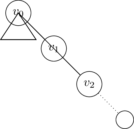
Figure 4 illustrates the canonical path \(r^*\). We focus on adversaries that seek to maximize the growth of \(\mathcal{T}^{(0)}\) by steering insertions to extend \(r^*\) over the \(Tk\) (flattened) insertion rounds. We refer to such adversaries as \(r^*\)-averse.

8.4 The Monotonic Structure of the Optimal Strategy \(\pi_{r^*}\) for the \(r^*\)-Averse Adversary↩︎

We now characterize the structure of the optimal policy \(\pi_{r^*}\) for the \(r^*\)-averse adversary. We show that, in both the adaptive and oblivious settings, the adversary may be restricted without loss of generality to a simple monotone family of strategies. First, among all \(\sigma\)-smooth distributions on \([0,1]\), it is optimal to choose a uniform distribution over an interval of length \(1/\sigma\). Second, the support of this interval may be assumed to move weakly to the right over time. Together, these two properties imply that the optimal strategy is fully described by a sequence of nonnegative shifts.

We formalize these two structural properties below.

The two lemmas imply that the optimal \(r^*\)-averse strategy has a simple canonical form. It starts from the leftmost feasible interval and then shifts it weakly to the right over time. More precisely, the optimal strategy may be written as \[\begin{align} \mathcal{D}_1 &:= \mathcal{U}\!\left(\left[0,\frac{1}{\sigma}\right]\right), \\ \mathcal{D}_t &= \mathcal{D}_{t-1} + \epsilon_t, \qquad t \ge 2, \end{align}\] for some sequence of shifts \(\epsilon_t \ge 0\).

The distinction between the adaptive and oblivious settings lies only in how these shifts are chosen. In the adaptive case, \(\epsilon_t\) may depend on the observed history up to round \(t-1\), in particular on the running maximum \(\max\{x_1,\dots,x_{t-1}\}\) and the remaining horizon. In the oblivious case, the full sequence \((\epsilon_t)_{t=2}^{Tk}\) is fixed a priori.

An analogous structural property holds for any choice of canonical path. For a general path, the optimal policy adapts to its branching pattern, and the resulting evolution may not admit the rightward monotonicity description. Nevertheless, by symmetry among root-to-leaf paths, focusing on \(r^*\)—which always follows the right child—is without loss of generality and naturally yields a monotone rightward-shifting strategy.

We now analyze the height of the data structure under adaptive and oblivious \(r^*\)-averse adversaries, assuming the monotone optimal strategy \(\pi_{r^*}\).

To make the dependence on the current maximum and the remaining horizon explicit, we formulate a Bellman optimality equation for the choice of \(\mathcal{D}_t\) at each round. For analytical convenience, we first discretize the action space: instead of distributions supported on the continuous interval \([0,1]\), we consider distributions supported on a grid of \(N\) points. This converts the Bellman recursion into a standard finite dynamic programming problem. We analyze the discrete model and then lift the resulting insights and bounds to the original continuous setting.

8.5 Adaptive \(r^*\)-averse Adversary↩︎

We now analyze the expected height of \(\mathcal{T}^{(0)}\) under an \(r^*\)-averse adaptive adversary following the monotone strategy \(\pi_{r^*}\).

Let \(M_t := \max\{x_1,\dots,x_t\}\) denote the running maximum up to round \(t\). Under the canonical form of the strategy, each distribution \(\mathcal{D}_t\) is uniform over an interval of length \(1/\sigma\), i.e., \[\mathcal{D}_t = \mathcal{U}([a_t,\, a_t + \tfrac{1}{\sigma}]),\] where \(0 = a_1 \le a_2 \le \cdots \le a_{Tk} \le 1 - \tfrac{1}{\sigma}\), and the shifts \(a_t\) are chosen adaptively based on the history through \(M_{t-1}\).

At round \(t\), the tree height increases if and only if \(x_t > M_{t-1}\). Since \(x_t \sim \mathcal{U}([a_t, a_t + \tfrac{1}{\sigma}])\), the probability of this event depends on how much of the support lies to the right of \(M_{t-1}\). Define \[p_t \doteq \bigl(a_t + \tfrac{1}{\sigma} - M_{t-1}\bigr)_+,\] which is the length of the portion of the support of \(\mathcal{D}_t\) that lies above \(M_{t-1}\). Then \[\Pr(x_t > M_{t-1} \mid M_{t-1}) = \sigma\, p_t.\]

Under the \(r^*\)-averse reduction, the height of \(\mathcal{T}^{(0)}\) is exactly the length of the canonical path \(r^*\), so it is convenient to denote this quantity by \(L_{Tk}\). Since each extension of \(r^*\) corresponds to a new record, we have \[L_{Tk} = 1 + \sum_{t=2}^{Tk} \mathbf{1}\{x_t > M_{t-1}\}.\] Taking expectations and applying the law of total expectation yields \[\begin{align} \mathbb{E}[\texttt{Height}(\mathcal{T}^{(0)})] = \mathbb{E}[L_{Tk}] = 1 + \sum_{t=2}^{Tk} \mathbb{E}\!\left[\Pr(x_t > M_{t-1} \mid M_{t-1})\right] = 1 + \sum_{t=2}^{Tk} \sigma\, \mathbb{E}[p_t]. \label{eq:adaptiveeq1} \end{align}\tag{5}\]

After the adversary selects \(\mathcal{D}_t\), a sample \(x_t \sim \mathcal{D}_t\) is drawn. If \(x_t > M_{t-1}\), then the running maximum increases to \(M_t = x_t\), and the interval \((M_{t-1},x_t]\) becomes inactive for all future rounds. Thus, each increase of the running maximum permanently removes part of the active range.

Since these increments are disjoint and contained in \([0,1]\), their total length is at most \(1\). Equivalently, with the convention \(M_0=0\), \[\sum_{t=1}^{Tk} (x_t-M_{t-1})_+ = M_{Tk} \le 1.\] Taking expectations yields \[\mathbb{E}\!\left[\sum_{t=1}^{Tk} (x_t-M_{t-1})_+\right] \le 1.\]

Moreover, conditional on \(M_{t-1}\), the portion of \(\mathcal{D}_t\) lying to the right of \(M_{t-1}\) has length \(p_t\) and density \(\sigma\). Therefore, \[\mathbb{E}\!\left[(x_t-M_{t-1})_+ \mid M_{t-1}\right] = \int_0^{p_t} \sigma x\,dx = \frac{\sigma p_t^2}{2}.\] Summing over \(t\) and applying the law of total expectation gives \[\begin{align} \mathbb{E}\!\left[\sum_{t=1}^{Tk} (x_t-M_{t-1})_+\right] &= \mathbb{E}\!\left[\sum_{t=1}^{Tk} \mathbb{E}\!\left[(x_t-M_{t-1})_+ \mid M_{t-1}\right]\right], \nonumber \\ &= \mathbb{E}\!\left[\sum_{t=1}^{Tk} \int_0^{p_t} \sigma x\,dx\right], \nonumber \\ &= \frac{1}{2}\,\mathbb{E}\!\left[\sum_{t=1}^{Tk} \sigma p_t^2\right] \le 1. \label{eq:adaptiveeq2} \end{align}\tag{6}\] Hence, \(\mathbb{E}\!\left[\sum_{t=1}^{Tk} \sigma p_t^2\right] \le 2.\)

We now combine the equation 5 and inequality 6 . We have \[\begin{align} \sum_{t=1}^{Tk}\sigma p_t &\le \sqrt{\left(\sum_{t=1}^{Tk}1\right)\left(\sum_{t=1}^{Tk}\sigma^2 p_t^2\right)} \\ &= \sqrt{Tk}\,\sqrt{\sigma\sum_{t=1}^{Tk}\sigma p_t^2}, \end{align}\] where the inequality follows from Cauchy–Schwarz. Taking expectations, we obtain \[\begin{align} \sum_{t=1}^{Tk}\sigma\,\mathbb{E}[p_t] &= \mathbb{E}\!\left[\sum_{t=1}^{Tk}\sigma p_t\right] \\ &\le \sqrt{Tk}\,\mathbb{E}\!\left[\sqrt{\sigma\sum_{t=1}^{Tk}\sigma p_t^2}\right] \\ &\overset{(a)}\le \sqrt{Tk}\,\sqrt{\sigma\,\mathbb{E}\!\left[\sum_{t=1}^{Tk}\sigma p_t^2\right]} \\ &\le \sqrt{2\sigma Tk}, \end{align}\] where the inequality (a) follows from Jensen’s inequality. Substituting into 5 yields \[\mathbb{E}[\texttt{Height}(\mathcal{T}^{(0)})] \le 1+\sqrt{2\sigma Tk} = O(\sqrt{\sigma Tk}).\]

8.6 Oblivious \(r^*\)-averse Adversary↩︎

We now turn to the oblivious \(r^*\)-averse adversary. In this setting, the distributions \(\mathcal{D}_1,\dots,\mathcal{D}_{Tk}\) are fixed in advance, and only then are the samples \(x_1,\dots,x_{Tk}\) drawn. Accordingly, the shifts \(\epsilon_t\) are no longer functions of the running maximum \(M_{t-1}\), but are instead chosen a priori.

This distinction changes the structure of the analysis. We therefore begin with the simpler case in which all supports \(\mathcal{D}_t=[a_t,a_t+\frac{1}{\sigma}]\) have a nonempty common intersection, and then study a concrete example within this class that already exhibits the sharp \(\Theta(\sqrt{Tk})\) behavior.

8.6.0.1 Intersecting supports.

We say that the supports intersect if \[\bigcap_{t=1}^{Tk} \left[a_t,\,a_t+\frac{1}{\sigma}\right] \neq \emptyset.\] Assuming the strategy is monotone, the left endpoints satisfy \[0 = a_1 \le a_2 \le \cdots \le a_{Tk} \le 1-\frac{1}{\sigma}.\] Under this monotonicity, the intersection condition is equivalent to \[a_{Tk} \le \frac{1}{\sigma}.\]

For such a sequence, the expected height of \(\mathcal{T}^{(0)}\) admits an exact integral representation. Indeed, \[\begin{align} \mathbb{E}[\texttt{Height}(\mathcal{T}^{(0)})] &= \sum_{t=1}^{Tk} \Pr(x_t > M_{t-1}) \nonumber\\ &= \sum_{t=1}^{Tk} \int_{a_t}^{a_t+\frac{1}{\sigma}} \sigma \,\Pr(M_{t-1} < x)\,dx \nonumber\\ &= \sum_{t=1}^{Tk} \int_{a_t}^{a_t+\frac{1}{\sigma}} \sigma \,\prod_{t'=1}^{t-1}\Pr(x_{t'} < x)\,dx \nonumber\\ &= \sum_{t=1}^{Tk} \int_{0}^{1} \prod_{t'=1}^{t-1}\Pr\!\left(x_{t'} < a_t+\frac{u}{\sigma}\right)\,du. \label{eq:obliviouseq1} \end{align}\tag{7}\] Here we used the fact that, once the oblivious adversary fixes the intervals, the samples are independent.

The expression inside the product can be computed explicitly. For every \(t'<t\), since \(a_t\ge a_{t'}\), we have \[\Pr\!\left(x_{t'} < a_t+\frac{u}{\sigma}\right) = \min\!\left\{1,\,u+\sigma(a_t-a_{t'})\right\}.\] Substituting this into 7 yields \[\begin{align} \mathbb{E}[\texttt{Height}(\mathcal{T}^{(0)})] &= \sum_{t=1}^{Tk} \int_0^1 \prod_{t'=1}^{t-1} \min\!\left\{1,\,u+\sigma(a_t-a_{t'})\right\}\,du. \label{eq:oblivious-min-form} \end{align}\tag{8}\]

To upper bound this expression, fix \(t\) and \(u\), and define the active set \[\mathcal{B}_t(u) \doteq \left\{t'<t:\;\sigma(a_t-a_{t'}) < 1-u\right\}.\] For indices \(t'\notin \mathcal{B}_t(u)\), the quantity \(u+\sigma(a_t-a_{t'})\) is at least \(1\), so the corresponding factor in the product is exactly \(1\). Therefore only the active indices matter, and \[\prod_{t'=1}^{t-1} \min\!\left\{1,\,u+\sigma(a_t-a_{t'})\right\} = \prod_{t' \in \mathcal{B}_t(u)} \left(u+\sigma(a_t-a_{t'})\right).\]

We now bound this product exponentially. Since every active factor lies in \([0,1]\), the inequality \[y \le e^{-(1-y)} \qquad\text{for all } y \in [0,1]\] implies \[\prod_{t' \in \mathcal{B}_t(u)} \left(u+\sigma(a_t-a_{t'})\right) \le \exp\!\left( -\sum_{t' \in \mathcal{B}_t(u)} \left(1-u-\sigma(a_t-a_{t'})\right) \right).\] Defining \[R_t(u) \doteq \sum_{t' \in \mathcal{B}_t(u)} \left(1-u-\sigma(a_t-a_{t'})\right),\] we obtain \[\begin{align} \mathbb{E}[\texttt{Height}(\mathcal{T}^{(0)})] &\le \sum_{t=1}^{Tk}\int_0^1 e^{-R_t(u)}\,du. \label{eq:oblivious-final-bound} \end{align}\tag{9}\]

We next instantiate this bound on a concrete monotone example: \[a_t=\frac{t-1}{\sigma Tk}, \qquad t=1,\dots,Tk.\] This sequence clearly satisfies \[a_{Tk}=\frac{Tk-1}{\sigma Tk}\le \frac{1}{\sigma},\] so all supports intersect. Moreover, \[\sigma(a_t-a_{t'})=\frac{t-t'}{Tk}.\] Hence, for fixed \(t\) and \(u\), the active set becomes \[\mathcal{B}_t(u) = \left\{t'<t:\frac{t-t'}{Tk}<1-u\right\},\] which is equivalent to \[t' > t-Tk(1-u).\] If we let \[N_t(u)\doteq |\mathcal{B}_t(u)|,\] then \[N_t(u)=\min\!\left\{t-1,\left\lfloor Tk(1-u)\right\rfloor\right\}.\] In this case, the active gaps are precisely \[\frac{1}{Tk},\frac{2}{Tk},\dots,\frac{N_t(u)}{Tk},\] so the exponent takes the explicit form \[\begin{align} R_t(u) &= \sum_{m=1}^{N_t(u)}\left(1-u-\frac{m}{Tk}\right) \nonumber\\ &= N_t(u)(1-u)-\frac{N_t(u)(N_t(u)+1)}{2Tk}. \label{eq:linear-Rt} \end{align}\tag{10}\] Substituting this into 9 , we get \[\begin{align} \mathbb{E}[\texttt{Height}(\mathcal{T}^{(0)})] &\le \sum_{t=1}^{Tk}\int_0^1 \exp\!\left( -N_t(u)(1-u)+\frac{N_t(u)(N_t(u)+1)}{2Tk} \right)\,du. \label{eq:linear-upper} \end{align}\tag{11}\]

We now show that the right-hand side of 11 is \(O(\sqrt{Tk})\). The case \(t=1\) is trivial, since \(\Pr(x_1>M_0)=1\). So fix \(t\ge 2\). We split the integral into two regions according to whether \(N_t(u)=t-1\) or \(N_t(u)=\lfloor Tk(1-u)\rfloor\).

On the first region, \[0\le u\le 1-\frac{t-1}{Tk},\] we have \(N_t(u)=t-1\), and therefore \[R_t(u) = (t-1)(1-u)-\frac{t(t-1)}{2Tk}.\] Thus, \[\begin{align} \int_0^{1-\frac{t-1}{Tk}} e^{-R_t(u)}\,du &= \int_0^{1-\frac{t-1}{Tk}} \exp\!\left( -(t-1)(1-u)+\frac{t(t-1)}{2Tk} \right)\,du. \end{align}\] Making the change of variables \(z=1-u\), this becomes \[\begin{align} e^{\frac{t(t-1)}{2Tk}} \int_{\frac{t-1}{Tk}}^{1} e^{-(t-1)z}\,dz &\le e^{\frac{t(t-1)}{2Tk}} \int_{\frac{t-1}{Tk}}^{\infty} e^{-(t-1)z}\,dz \nonumber\\ &= \frac{1}{t-1} \exp\!\left( -\frac{(t-1)(t-2)}{2Tk} \right). \label{eq:linear-upper-part1} \end{align}\tag{12}\]

On the second region, \[1-\frac{t-1}{Tk}\le u\le 1,\] we have \[N_t(u)=\lfloor Tk(1-u)\rfloor.\] Letting \(v=1-u\), we obtain \(0\le v\le \frac{t-1}{Tk}\) and \[N_t(u)=\lfloor Tkv\rfloor.\] Using 10 , we can write \[R_t(u) = \lfloor Tkv\rfloor\,v - \frac{\lfloor Tkv\rfloor(\lfloor Tkv\rfloor+1)}{2Tk}.\] Since \(\lfloor Tkv\rfloor \ge Tkv-1\), it follows that \[R_t(u)\ge \frac{Tk}{2}v^2-v.\] Therefore, \[\begin{align} \int_{1-\frac{t-1}{Tk}}^1 e^{-R_t(u)}\,du &\le \int_0^1 \exp\!\left(-\frac{Tk}{2}v^2+v\right)\,dv \nonumber\\ &\le e\int_0^1 e^{-\frac{Tk}{2}v^2}\,dv = O\!\left(\frac{1}{\sqrt{Tk}}\right). \label{eq:linear-upper-part2} \end{align}\tag{13}\]

Combining the two regions, we conclude that for every \(t\ge 2\), \[\int_0^1 e^{-R_t(u)}\,du \le \frac{1}{t-1} \exp\!\left( -\frac{(t-1)(t-2)}{2Tk} \right) + O\!\left(\frac{1}{\sqrt{Tk}}\right).\] Summing this bound over \(t=2,\dots,Tk\), the first term contributes at most \(O(\log Tk)\), while the second contributes \(O(\sqrt{Tk})\). Together with the \(t=1\) term, this proves \[\mathbb{E}[\texttt{Height}(\mathcal{T}^{(0)})]=O(\sqrt{Tk}).\]

We next show that this order is attained by the same example. Returning to the exact formula 8 , fix any \(t\ge 2\sqrt{Tk}\) and restrict the integral to the interval \[u\in\left[1-\frac{1}{\sqrt{Tk}},\,1\right].\] If \(t'<t-\sqrt{Tk}\), then \[u+\sigma(a_t-a_{t'}) = u+\frac{t-t'}{Tk} \ge 1-\frac{1}{\sqrt{Tk}}+\frac{\sqrt{Tk}}{Tk} =1,\] so the corresponding factor is exactly \(1\). For the remaining at most \(\sqrt{Tk}\) indices, each factor is at least \[u\ge 1-\frac{1}{\sqrt{Tk}}.\] Hence, \[\begin{align} \Pr(x_t>M_{t-1}) &= \int_0^1 \prod_{t'=1}^{t-1} \min\!\left\{1,u+\frac{t-t'}{Tk}\right\}\,du \nonumber\\ &\ge \int_{1-1/\sqrt{Tk}}^1 \left(1-\frac{1}{\sqrt{Tk}}\right)^{\sqrt{Tk}}\,du \nonumber\\ &= \frac{1}{\sqrt{Tk}} \left(1-\frac{1}{\sqrt{Tk}}\right)^{\sqrt{Tk}} = \Omega\!\left(\frac{1}{\sqrt{Tk}}\right). \end{align}\] Summing this lower bound over all \(t=2\sqrt{Tk},\dots,Tk\), we obtain \[\mathbb{E}[\texttt{Height}(\mathcal{T}^{(0)})]=\Omega(\sqrt{Tk}).\]

We have therefore shown that for the example \[a_t=\frac{t-1}{\sigma Tk},\] the expected height satisfies \[\mathbb{E}[\texttt{Height}(\mathcal{T}^{(0)})]=\Theta(\sqrt{Tk}).\] Since oblivious adversaries are a subclass of adaptive adversaries, the adaptive upper bound \(O(\sqrt{Tk})\) also applies to the oblivious optimum. Combined with the above construction, this shows that the optimal oblivious \(r^*\)-averse adversary also achieves \(\Theta(\sqrt{Tk})\).

8.7 Oblivious Random-Order Adversary↩︎

This follows from the fact that hyperplanes \(\psi_t\) arrive in uniformly random order within each direction \(\gamma_i \in \Gamma\), and layers evolve independently. The bound is implied by the classical Binary Search Tree result:

9 Warm-Up: Example Insertion and Sampling in \(2\)-Dimensions (5.2)↩︎

To illustrate the use of the structure, consider the warm-up case where two hyperplanes arrive at time \(t\): \(\psi_{1,t} : x^{(0)} = c^{(0)}_t\) and \(\psi_{2,t} : x^{(1)} = c^{(1)}_t\). These partition the domain \([0,1)^2\) into four rectangular regions \(\rho_{i,t}\), each assigned a \(\text{reward function parameters}\) \(f_t(\rho_{i,t})\). The regions are:

\[\begin{array}{ll} \rho_{1,t}: [0{:}c^{(0)}_t][c^{(1)}_t{:}1],\; f_t(\rho_{1,t}) \quad & \rho_{2,t}: [c^{(0)}_t{:}1][c^{(1)}_t{:}1],\; f_t(\rho_{2,t}) \\ \rho_{3,t}: [0{:}c^{(0)}_t][0{:}c^{(1)}_t],\; f_t(\rho_{3,t}) \quad & \rho_{4,t}: [c^{(0)}_t{:}1][0{:}c^{(1)}_t],\; f_t(\rho_{4,t}) \end{array}\]

Each region \(\rho_{i,t}\) is inserted by identifying all \(v_0 \in \mathcal{T}^{(0)}\) whose horizontal range \(\texttt{Int}(v_0)\) intersects the horizontal interval of \(\rho_{i,t}\). Depending on the nature of the intersection:

• If \(\texttt{Int}(v_0)\) is intersects, the vertical interval is inserted into \(\mathcal{T}^{(1)}_{v_0}\) (regular insertion tree).

• If \(\texttt{Int}(v_0)\) is fully contained in the region’s horizontal interval, the update is deferred to \(\mathcal{L}^{(1)}_{v_0}\) or \(\mathcal{R}^{(1)}_{v_0}\), depending on the subtree alignment.

In all cases, the cumulative reward vector \(f_t(\rho_{i,t})\) is added to the corresponding node in the second-level tree, ensuring each rectangular region contributes correctly to later queries.

9.0.0.1 Handling \(\texttt{Insert}(\rho_{1,t})\) Query:

We insert the region \(\rho_{1,t} = [0{:}c^{(0)}_t][c^{(1)}_t{:}1]\) following the hierarchical structure of \(\mathcal{T}\). First, we refine the first-level tree \(\mathcal{T}^{(0)}\) to align with the endpoints \(0\) and \(c^{(0)}_t\), by locating the leaves containing each and splitting the corresponding leaves if needed. Let \(l_0\) and \(u_0\) denote the resulting leaves. We then define the upward paths \(p_{l_0}\) and \(p_{u_0}\) to the root and compute the lowest common ancestor \(v_{l_0,u_0} = \texttt{First\_Common\_Ancestor}(l_0, u_0)\). All nodes in \(p_{l_0} \cup p_{u_0}\) have horizontal ranges intersecting \([0{:}c^{(0)}_t]\), and the subtree of \(v_{l_0,u_0}\) contains all nodes fully contained in the interval.

We insert the vertical interval \([c^{(1)}_t{:}1]\) into each second-level tree according to the position of the corresponding \(v_0 \in \mathcal{T}^{(0)}\). For all \(v_0 \in p_{l_0} \cup p_{u_0}\), the insertion is regular into \(\mathcal{T}^{(1)}_{v_0}\) because the \(\texttt{Int}(v_0)\) intersects the horizontal interval of the inserted region. To identify lazy insertions, we consider nodes \(v_0 \in p_{l_0} \setminus p_{v_{l_0,u_0}}\) whose right child is not on that path, and nodes \(v_0 \in p_{u_0} \setminus p_{v_{l_0,u_0}}\) whose left child is not on that path. These are the roots of sibling subtrees entirely contained in \([0{:}c^{(0)}_t]\) and thus suitable for lazy updates.

Formally, we insert into \(\mathcal{R}^{(1)}_{v_0}\) if \[v_0 \in p_{l_0} \setminus p_{v_{l_0,u_0}} \quad \text{and} \quad \texttt{Right\_child}(v_0) \notin p_{l_0} \setminus p_{v_{l_0,u_0}},\] and into \(\mathcal{L}^{(1)}_{v_0}\) if \[v_0 \in p_{u_0} \setminus p_{v_{l_0,u_0}} \quad \text{and} \quad \texttt{Left\_child}(v_0) \notin p_{u_0} \setminus p_{v_{l_0,u_0}}.\]

Lazy insertions defer propagation of contributions to query time, allowing efficient updates without redundant insertions across multiple second-level structures. This process naturally extends to higher dimensions by recursively inserting projections along each axis across the tree layers.

Specifically, when inserting \([c^{(1)}_t{:}1]\) into a regular insertion tree \(\mathcal{T}^{(1)}_{v_0}\), we first locate the leaves that contain the endpoints \(c^{(1)}_t\) and \(1\), and refine them by splitting their intervals. This introduces two new child nodes per leaf, converting each into an internal node and designating the new children as leaves. We refer to the resulting leaves containing \(c^{(1)}_t\) and \(1\) as \(l_1\) and \(u_1\), respectively. We then define the upward paths \(p_{l_1}\) and \(p_{u_1}\) from \(l_1\) and \(u_1\) to the root of \(\mathcal{T}^{(1)}_{v_0}\), and identify their first common ancestor \(v_{l_1,u_1} = \texttt{First\_Common\_Ancestor}(l_1, u_1)\). We traverse \(p_{l_1} \cup p_{u_1}\) bottom-up to update the cumulative reward vectors, as described next. The procedure for inserting into lazy insertion data structures follows the same logic, with one important distinction: the update to the cumulative reward vectors differs slightly as detailed in the next section.

9.0.0.2 Handling \(\texttt{Update}(\rho_{1,t})\) Query:

Once \(\rho_{1,t}\) is inserted, we update the cumulative reward vectors in all second-level structures where its vertical interval \([c^{(1)}_t{:}1]\) was inserted—either regularly or lazily—using with the \(\text{reward function parameters}\) vector \(f_t(\rho_{1,t})\). This update follows the standard regular and lazy weight update mechanisms for interval trees [13], extended to vector-valued cumulative rewards as regular and lazy \(\text{reward function parameters}\) updates. Unlike lazy insertions, which defer interval insertions, lazy \(\text{reward function parameters}\) updates apply to reward vectors in second-level trees. While the update routine is structurally similar across regular and lazy insertion trees with minor implementation differences depending on the data structure type.

• Updating Regular Insertion \(\texttt{Interval Tree}\)s: For each node \(v_0 \in p_{l_0} \cup p_{u_0}\) where regular insertion occurred, we update the cumulative reward vector \(\vec{r}_{v_0,v_1}\) for every node \(v_1 \in \mathcal{T}^{(1)}_{v_0}\) whose vertical range \(\texttt{Int}(v_1)\) intersects the interval \([c^{(1)}_t{:}1]\). The update adds the contribution of the region \(\rho_{1,t}\) with its \(\text{reward function parameters}\) \(f_t(\rho_{1,t})\) over the intersected subregion \(\rho' = [\texttt{Int}(v_0) \cap [0{:}c^{(0)}_t]][\texttt{Int}(v_1) \cap [c^{(1)}_t{:}1]],\) which captures the portion of \(\rho_{1,t}\) aligned with the rectangular region defined by \(v_0\) and \(v_1\).

  To implement this, we first locate the leaves \(l_1\) and \(u_1\) in \(\mathcal{T}^{(1)}_{v_0}\) that contain the endpoints \(c^{(1)}_t\) and \(1\), respectively. We then traverse the paths \(p_{l_1}\) and \(p_{u_1}\) to the root, and for each node \(v_1\) along \(p_{l_1} \cup p_{u_1}\), we perform the update: \[\vec{r}_{v_0,v_1} \gets \vec{r}_{v_0,v_1} + \vec{A}_{\rho'},\] where \(\vec{A}_{\rho'}\) is the vector representation of the cumulative reward over \(\rho'\),i.e \(\vec{r}(\rho')\) with the \(f_t(\rho_{1,t})\) as the coefficient vector.

  Now, similar to our general strategy for efficient updates, we apply a lazy propagation scheme to vertical intervals in \(\mathcal{T}^{(1)}_{v_0}\), specifically targeting those subtrees whose vertical range \(\texttt{Int}(v_1)\) is fully contained within the vertical interval of the region \(\rho_{1,t}\). This follows the same logic as the lazy insertion mechanism.

  To implement this, we traverse the truncated paths \(p_{l_1} \setminus p_{v_{l_1,u_1}}\) and \(p_{u_1} \setminus p_{v_{l_1,u_1}}\). During each traversal, we propagate the update message \(f_t(\rho_{1,t})\), referred to as the lazy \(\text{reward function parameters}\) update message, to specific children of nodes along the path, provided those children are not themselves on the path. The cumulative lazy updates received by a node \(v_1\) from its parent in \(\mathcal{T}^{(1)}_{v_0}\) are stored in \(\texttt{Lazy\_Update\_Message}_{v_0,v_1}\).

  In particular, for each node \(v_1 \in p_{l_1} \setminus p_{v_{l_1,u_1}}\), we send a lazy \(\text{reward function parameters}\) update message to its right child \(\texttt{Right\_child}(v_1)\) if \(\texttt{Right\_child}(v_1) \notin p_{l_1} \setminus p_{v_{l_1,u_1}},\) by setting \[\texttt{Lazy\_Update\_Message}_{v_0, \texttt{Right\_child}(v_1)} \gets \texttt{Lazy\_Update\_Message}_{v_0, \texttt{Right\_child}(v_1)} + f_t(\rho_{1,t}).\]

  Likewise, for each node \(v_1 \in p_{u_1} \setminus p_{v_{l_1,u_1}}\), we send a lazy \(\text{reward function parameters}\) update message to its left child \(\texttt{Left\_child}(v_1)\) if \(\texttt{Left\_child}(v_1) \notin p_{u_1} \setminus p_{v_{l_1,u_1}},\) by setting \[\texttt{Lazy\_Update\_Message}_{v_0, \texttt{Left\_child}(v_1)} \gets \texttt{Lazy\_Update\_Message}_{v_0, \texttt{Left\_child}(v_1)} + f_t(\rho_{1,t}).\]

  These lazy update messages accumulated at each node encode the \(\text{reward function parameters}\)s of all regions whose contributions affect the entire subtree rooted at either the left or right child. Since these contributions are additive, we can aggregate the corresponding vectors and defer integration until propagation, ensuring correctness and efficiency in handling lazy updates.

• Updating Lazy Insertion \(\texttt{Interval Tree}\)s:

  For lazy insertions, the update routine is identical for both \(\mathcal{L}^{(1)}_{v_0}\) and \(\mathcal{R}^{(1)}_{v_0}\). As in the case of regular insertion trees, updating a lazy insertion tree involves locating the leaves \(l_1\) and \(u_1\), and traversing the nodes \(w_1 \in p_{l_1} \cup p_{u_1}\) to update their cumulative reward vectors by integrating \(f_t(\rho_{1,t})\) over appropriate rectangles \(\rho''\). Specifically, for each such node we perform the update: \[\vec{r}_{v_0,w_1} \gets \vec{r}_{v_0,w_1} + \vec{A}_{\rho''},\] where \(\rho'' = [\texttt{Int}(v_0)][\texttt{Int}(w_1) \cap [c^{(1)}_t{:}1]]\) denotes the subregion over which lazy integration is performed. Unlike the regular insertion case, the horizontal component of the integration is not restricted to the intersection with the horizontal interval of \(\rho_{1,t}\); rather, it is fixed to \(\texttt{Int}(v_0)\), since all affected subregions are fully contained within this range. This ensures that the contributions stored in lazy structures are correctly computed and remain scalable for future query processing.

  Lazy \(\text{reward function parameters}\) update messages are also handled in the same manner as in regular insertion trees. That is, we send \(f_t(\rho_{1,t})\) as a lazy message \(\texttt{Lazy\_Update\_Message}\) to those nodes whose vertical range is fully contained within the vertical interval of \(\rho_{1,t}\).

In both regular and lazy insertion structures, lazy update messages are propagated to their corresponding subtrees during leaf location in each second-level interval tree. Specifically, while locating a leaf node \(v_1\) in a second-level tree associated with a node \(v_0 \in \mathcal{T}^{(0)}\), the algorithm retrieves the corresponding lazy message \(\texttt{Lazy\_Update\_Message}_{v_0,v_1}\), which encodes an \(\text{reward function parameters}\) vector. It then integrates this vector over the appropriate region and propagates the resulting update downward through the subtree rooted at \(v_1\). The full procedure is detailed in Appendix 10.5.

Next we discuss the structural properties of our data structure that allows efficient sampling.

9.1 Structural Properties of \(\mathcal{T}\)↩︎

9.1.0.1 Main Structure:

The following observation clarifies the properties maintained during insertion, specifically how a region \(\rho\) is handled by the data structure upon insertion.

In the following, we describe how our hierarchical data structure supports online learning algorithms in drawing an action at each round with the correct probability. This is achieved by first identifying an atomic region with probability proportional to its cumulative reward, as maintained in the data structure.

9.1.0.2 Uniqueness and Completeness of the Information in the Data Structures Along the Paths:

Let \(v_0 \in \mathcal{T}^{(0)}\) be a node. We construct the set \(\mathcal{S}_{v_0}^{(1)}\), which includes the regular insertion tree \(\mathcal{T}^{(1)}_{v_0}\) as well as the corresponding lazy data structures of all ancestors of \(v_0\) along the path \(p_{v_0}\) toward the root. Specifically, for each ancestor \(v_0'\) of \(v_0\), we include \(\mathcal{L}^{(1)}_{v_0'}\) in \(\mathcal{S}_{v_0}^{(1)}\) if \(v_0\) lies in the left subtree of \(v_0'\), and \(\mathcal{R}^{(1)}_{v_0'}\) otherwise. This construction ensures that, for each node \(v_0' \in p_{v_0}\), exactly one second-level data structure—either regular or lazy—is included in \(\mathcal{S}_{v_0}^{(1)}\), which we denote by \(S^{(1)}_{v_0'}\).

The following Lemmas 3 and 4 together guarantee that: (i) every region intersecting \(\texttt{Int}(v_0)\) and influencing it is covered by some structure in \(\mathcal{S}_{v_0}^{(1)}\); and (ii) each such region is stored in exactly one of these structures.

We now describe how our drawing algorithm operates, assuming all required structural properties established thus far.

9.2 Drawing \(x_t\) via \(\texttt{Draw}(t)\)↩︎

As described above, the \(\texttt{Draw}(t)\) query samples an atomic region \(\rho= [c^{(0)}_{t_1}:c^{(0)}_{t_2}][c^{(1)}_{t_1}:c^{(1)}_{t_2}] \in F_t\) with probability proportional to its cumulative reward:

\[\Pr(\rho\gets \texttt{Draw}(t)) = \frac{r(\rho)}{\sum_{\rho' \in F_t} r(\rho')},\] where \(\Pr(\rho\gets \texttt{Draw}(t))\) is the probability of the drawing algorithm to return \(\rho\).

The sampling process consists of two stages: Horizontal Sampling followed by Vertical Sampling. In the horizontal sampling stage, the drawing algorithm selects an atomic horizontal interval \([c^{(0)}_{t_1} : c^{(0)}_{t_2}]\) by randomly traversing a root-to-leaf path in the auxiliary interval tree \(\mathcal{E}^{(0)}\), which encodes the horizontal structure of the action space. This traversal identifies a rectangular region whose horizontal interval is atomic and whose vertical interval spans the full range \([0:1]\) of the second coordinate of the action space. In the subsequent vertical sampling stage, the algorithm selects an atomic vertical interval \([c^{(1)}_{t_1} : c^{(1)}_{t_2}]\) within this subspace by traversing the corresponding auxiliary tree \(\mathcal{E}^{(1)}\). The combination of the selected atomic horizontal and vertical intervals uniquely determines an atomic region. At each stage, a cumulative reward retrieval query is used to compute the transition probabilities for navigating left or right within the auxiliary trees to get to the atomic intervals stored at the leaves at each stage. After sampling region \(\rho\) with the correct probability, this algorithm samples \(x_t\) within that region proportional to its cumulative reward using Hit-and-Run sampling algorithm.

9.2.0.1 Cumulative Reward Retrieval \(\texttt{CReward}(.)\) Query:

This query is responsible for retrieving the cumulative reward of the queried region while drawing. Although the \(\texttt{CReward}\) routine can handle arbitrary rectangular queries, the \(\texttt{Draw}\) algorithm only invokes it for two specific types of structured regions, denoted by \(\texttt{CReward}^{(0)}\) and \(\texttt{CReward}^{(1)}\). The query \(\texttt{CReward}^{(0)}(\rho_1: [x^{(0)}_1:x^{(0)}_2][0:1])\), used during horizontal sampling, retrieves the cumulative reward over a rectangular region with horizontal interval \([x^{(0)}_1:x^{(0)}_2]\) and full vertical range \([0:1]\). The endpoints of this horizontal interval are assumed to belong to the set \(c^{(0)}_{t'}\) for some \(t' \in [t]\), as defined by the adversary up to round \(t\). In contrast, the query \(\texttt{CReward}^{(1)}(\rho_2: [x'^{(0)}_1:x'^{(0)}_2][x^{(1)}_1:x^{(1)}_2])\), used during vertical sampling, retrieves the cumulative reward over a region whose horizontal interval \([x'^{(0)}_1:x'^{(0)}_2]\) corresponds to an atomic segment (i.e., a leaf in \(\mathcal{T}^{(0)}\)), and whose vertical interval \([x^{(1)}_1:x^{(1)}_2]\) has endpoints in \(c^{(1)}_{t'}\) for \(t' \in [t]\). Both types of queries are efficiently supported by the hierarchical interval tree \(\mathcal{T}\), including its regular and lazy insertion structures.

To compute \(\texttt{CReward}^{(0)}(\rho_1: [x^{(0)}_1:x^{(0)}_2][0:1])\), the algorithm first identifies the leaves \(l_0\) and \(u_0\) in \(\mathcal{T}^{(0)}\) that contain \(x^{(0)}_1\) and \(x^{(0)}_2\), respectively, and determines their first common ancestor \(v_{l_0,u_0}\). By construction, the horizontal interval \([x^{(0)}_1:x^{(0)}_2]\) is fully contained in \(\texttt{Int}(v_{l_0,u_0})\). The algorithm then retrieves the cumulative reward over the rectangular region \([\texttt{Int}(v_{l_0,u_0})][0:1]\) and prunes away contributions from subregions that fall outside the query region \(\rho_1\).

Thanks to the structural guarantees provided by Lemmas 3 and 4, the cumulative reward over \([\texttt{Int}(v_{l_0,u_0})][0:1]\) is distributed across multiple second-level data structures, including both regular and lazy insertion trees associated with nodes whose horizontal ranges intersect or contain \(\texttt{Int}(v_{l_0,u_0})\). By Lemma 3, each contributing region is stored in exactly one such data structure, allowing the total to be computed by aggregating disjoint contributions from the set \(\mathcal{S}^{(1)}_{v_{l_0,u_0}}\), which includes:

• The cumulative reward vector \(\vec{r}_{v_{l_0,u_0}, \texttt{Root}(\mathcal{T}^{(1)}_{v_{l_0,u_0}})}\), stored at the root of the regular insertion tree \(\mathcal{T}^{(1)}_{v_{l_0,u_0}}\), which encodes the contribution of all regions whose vertical intervals intersect \(\texttt{Int}(v_{l_0,u_0})\);

• Scaled cumulative reward vectors stored at the roots of the lazy insertion trees \(\mathcal{L}^{(1)}_{v_0}\) or \(\mathcal{R}^{(1)}_{v_0}\), where each \(v_0 \in p_{v_{l_0,u_0}}\) is an ancestor whose horizontal range \(\texttt{Int}(v_0)\) fully contains \(\texttt{Int}(v_{l_0,u_0})\), and whose lazy subtree therefore contributes to the query region.

The algorithm then prunes the cumulative reward contributions corresponding to portions of the region \([\texttt{Int}(v_{l_0,u_0})][0:1]\) that fall outside the query rectangle \(\rho: [x^{(0)}_1:x^{(0)}_2][0:1]\). This pruning is performed in two symmetric passes. First, it traverses the nodes \(v_0 \in p_{l_0}\). For each such node, if the horizontal range of its left child \(\texttt{Int}(\texttt{Left\_child}(v_0))\) lies entirely outside the interval \([x^{(0)}_1:x^{(0)}_2]\), the algorithm subtracts the cumulative reward over the region \([\texttt{Int}(\texttt{Left\_child}(v_0))][0:1]\). This quantity is retrieved via a recursive call to \(\texttt{CReward}^{(0)}([\texttt{Int}(\texttt{Left\_child}(v_0))][0:1])\), where no further pruning is necessary. A symmetric pruning pass is applied along the path \(p_{u_0}\). For each node \(v_0 \in p_{u_0}\), if the horizontal range of its right child \(\texttt{Int}(\texttt{Right\_child}(v_0))\) does not intersect \([x^{(0)}_1:x^{(0)}_2]\), the cumulative reward over the region \([\texttt{Int}(\texttt{Right\_child}(v_0))][0:1]\) is subtracted. This procedure ensures that only the contribution from the queried region is retained in the final result. The complete implementation of the cumulative reward query \(\texttt{CReward}^{(0)}\) is detailed in Section 10.6.1.

The query \(\texttt{CReward}^{(1)}(\rho_2:[x'^{(0)}_1:x'^{(0)}_2][x^{(1)}_1:x^{(1)}_2])\) is handled in a manner similar to \(\texttt{CReward}^{(0)}\), with the main distinction arising from the structure of the queried region \(\rho_2\), whose horizontal interval \([x'^{(0)}_1:x'^{(0)}_2]\) is assumed to be atomic. Consequently, both endpoints of the horizontal interval are contained within a single leaf \(l_0 \in \mathcal{T}^{(0)}\), such that \(\texttt{Int}(l_0) = [x'^{(0)}_1:x'^{(0)}_2]\).

Given this atomic interval, the algorithm constructs the set \(\mathcal{S}^{(1)}_{l_0}\), consisting of the regular insertion tree \(\mathcal{T}^{(1)}_{l_0}\) and the lazy insertion trees associated with the ancestors of \(l_0\). Together, these structures maintain the vertical subdivision necessary for handling the query region \(\rho_2\).

Unlike the \(\texttt{CReward}^{(0)}\) case, however, the vertical interval \([x^{(1)}_1:x^{(1)}_2]\) does not span the full range \([0:1]\), and its endpoints may not align with any node boundaries in the second-level trees. This is due to the deferred insertion strategy used in maintaining the lazy insertion data structures: vertical intervals are incorporated only through scaling, and their endpoints may be distributed across multiple second-level trees.

As a result, each data structure in \(\mathcal{S}^{(1)}_{l_0}\) must be traversed to locate the leaves \(l_1\) and \(u_1\) containing \(x^{(1)}_1\) and \(x^{(1)}_2\), respectively. The algorithm then computes their first common ancestor—denoted \(v_{l_1,u_1}\) in regular insertion trees and \(w_{l_1,u_1}\) in lazy ones. It retrieves the cumulative reward over the region \([\texttt{Int}(l_0)][\texttt{Int}(v_{l_1,u_1})]\) (or \([\texttt{Int}(l_0)][\texttt{Int}(w_{l_1,u_1})]\)) and prunes it to match the exact query rectangle \(\rho_2\).

Since the endpoints \(x^{(1)}_1\) and \(x^{(1)}_2\) may lie in the interior of the ranges \(\texttt{Int}(l_1)\) and \(\texttt{Int}(u_1)\), additional leaf-level pruning and scaling is required. In lazy insertion trees, this is handled correctly by construction, as guaranteed by Corollary 2. For the regular insertion tree \(\mathcal{T}^{(1)}_{l_0}\), correctness is ensured by Lemma 6, which applies specifically because \(l_0\) is a leaf in \(\mathcal{T}^{(0)}\). In essence, once we are assured that \(l_0\) is a leaf, our update mechanism—particularly the way lazy \(\text{reward function parameters}\) update messages are propagated—allows us to treat \(\mathcal{T}^{(1)}_{l_0}\) similarly to a lazy insertion data structure. As a result, the same scalability and pruning guarantees hold. The full procedure for answering the cumulative reward query \(\texttt{CReward}^{(1)}\) is described in Section 10.6.2.

This structured decomposition, combined with the scalability of cumulative reward vectors and efficient detachment, enables \(\texttt{CReward}^{(1)}\) to support fast and accurate evaluation of cumulative rewards over sub-rectangles, as required by the \(\texttt{Draw}(t)\) routine. We now describe how the drawing algorithm employs these two subclasses of cumulative reward retrieval queries along with horizontal and vertical sampling to locate an atomic region with probability proportional to its cumulative reward.

9.2.0.2 Horizontal Sampling.

By the horizontal sampling step, the \(\texttt{Draw}(t)\) algorithm samples a region \(\rho_1 = [c^{(0)}_{t_1}:c^{(0)}_{t_2}][0:1]\) with probability proportional to \(r(\rho_1)/r([0:1][0:1])\), where the horizontal interval \([c^{(0)}_{t_1}:c^{(0)}_{t_2}]\) is atomic. To this end, the algorithm performs a randomized root-to-leaf traversal of the first-level auxiliary interval tree \(\mathcal{E}^{(0)}\). The leaf reached by this traversal corresponds to a rectangular region with atomic horizontal interval and full vertical range.

The traversal begins at the root node \(u_0 = \texttt{Root}(\mathcal{E}^{(0)})\). Then, while \(u_0\) remains an internal node, the algorithm sets \(u_0\) to its right child with probability \[\Pr(u_0 \gets \texttt{Right\_child}(u_0)) = \frac{r([\texttt{Int}(\texttt{Right\_child}(u_0))][0:1])}{r([\texttt{Int}(u_0)][0:1])},\] and to its left child with the complementary probability. The values \(r([\texttt{Int}(\texttt{Right\_child}(u_0))][0:1])\) are computed using the query \(\texttt{CReward}^{(0)}([\texttt{Int}(\texttt{Right\_child}(u_0))][0:1])\). The traversal continues until reaching a leaf \(l_0\), where \(\texttt{Int}(l_0) = [c^{(0)}_{t_1}:c^{(0)}_{t_2}]\).

9.2.0.3 Vertical Sampling.

Given the selected horizontal interval \(\texttt{Int}(l_0)\), we sample a vertical atomic interval to complete the region \(\rho_2\). This is done by traversing the auxiliary tree \(\mathcal{E}^{(1)}\) top-down. At each internal node \(u_1\), the next move is selected via: \[\Pr(u_1 \gets \texttt{Right\_child}(u_1)) = \frac{r([\texttt{Int}(l_0)][\texttt{Int}(\texttt{Right\_child}(u_1))])}{r([\texttt{Int}(l_0)][\texttt{Int}(u_1)])},\] and \(\Pr(u_1 \gets \texttt{Left\_child}(u_1)) = 1 - \Pr(u_1 \gets \texttt{Right\_child}(u_1))\). The cumulative reward values are computed using \(\texttt{CReward}^{(1)}\). This continues until reaching a leaf \(l_1\), yielding \(\texttt{Int}(l_1) = [c^{(1)}_{t_1}:c^{(1)}_{t_2}]\), and completing the sampled region \(\rho_2 = [\texttt{Int}(l_0)][\texttt{Int}(l_1)]\). This region \(\rho_2\) then will be returned as the drawn region \(\rho\). The detailed queries and their pseudocode implementations are provided in Appendices 10.

9.2.0.4 Sampling \(x_t\) within Region \(\rho\).

After sampling a region \(\rho\) with probability proportional to its cumulative reward, we now sample a point \(x_t \in \rho\) according to a distribution proportional to the cumulative reward within \(\rho\). Specifically, we aim to sample \(x_t\) with probability \[x_t \sim \frac{r(x)}{r(\rho)} = \frac{g(x, F_t(x))}{\int_{\rho}g(x, F_t(x))dx}.\] To accomplish this, we invoke the following result regarding the Hit-and-Run [32] algorithm:

We now verify that the conditions of Theorem 7 are satisfied in our setting. First, we assume that the mapping \(g(x, \cdot)\) is a log-concave polynomial and that the vector \(f_t\) is positive at every round, ensuring that the resulting function \(g(x, F_t(x))\) is log-concave. Second, since our action space \(\text{action parameter space}\) is a rectangular region, it is convex, and a membership oracle can be implemented efficiently via simple geometric checks. Therefore, we can apply the Hit-and-Run algorithm to sample \(x_t \in \rho\) in \(O(d^3)\) steps with high accuracy from the target distribution.

9.3 Correctness and Generalization↩︎

The correctness of all core operations—including \(\texttt{Insert}\), \(\texttt{Update}\), \(\texttt{CReward}\), and \(\texttt{Draw}\)—is formally and in detale established in Appendix 11. Appendix 12 then presents the generalization of our data structure to \(d\)-dimensions. This involves extending the hierarchical design so that each node at every level is augmented with two next-level structures corresponding to regular and lazy insertions. The structural properties proven in Section 9.1 carry over to this generalized setting.

10 Query Details and Implementations in \(2\)-Dimensions (5.2)↩︎

We now describe how to initialize the data structure and handle the queries introduced in Section 4. We begin with the insertion and update routines for an arbitrary rectangular region \(\rho= [x^{(0)}_1:x^{(0)}_2][x^{(1)}_1:x^{(1)}_2]\), which form the basis for maintaining \(\mathcal{T}\) at each time step. We then illustrate these procedures using the region \(\rho_{1,t} \in \mathcal{P}_t\) as a representative example. The same steps apply to all other regions in \(\mathcal{P}_t\) and, more generally, to any rectangular region.

10.1 Initialization:↩︎

We initialize the data structure \(\mathcal{T}\) by creating a two-dimensional \(\texttt{Interval Tree}\). This initialization involves constructing \(\mathcal{T}^{(0)}\) as a balanced \(\texttt{Interval Tree}\) that initially contains the single horizontal interval \([0,1)\), represented by a single node \(\texttt{Root}(\mathcal{T}^{(0)})\). Simultaneously, the associated second-level data structures \(\mathcal{T}^{(1)}\), \(\mathcal{L}^{(1)}\), and \(\mathcal{R}^{(1)}\) are initialized as \(\texttt{Interval Tree}\)s over the vertical interval \([0,1)\). Every time a new node is inserted into \(\mathcal{T}^{(0)}\), we follow the same initialization steps by creating its associated second-level lazy and regular insertion \(\texttt{Interval Tree}\)s.

10.2 Locating an Endpoint \(x^{(i)}\)↩︎

Many of the queries described below rely on a common subroutine: locating the leaf node in an \(\mathcal{T}^{(i)}\) whose interval contains a given endpoint \(x^{(i)}\). The search starts at the root \(\texttt{Root}(\mathcal{T}^{(i)})\) and recursively moves to the left or right child, depending on which subtree contains \(x^{(i)}\), until reaching a leaf representing the atomic interval that includes \(x^{(i)}\).

10.3 Locating the Smallest Interval Containing \([x^{(i)}_1{:}x^{(i)}_2]\)↩︎

Several queries require finding the node in \(\mathcal{T}^{(i)}\) whose interval is the smallest one that fully contains \([x^{(i)}_1{:}x^{(i)}_2]\). This node is the first common ancestor of the leaves \(l_i\) and \(h_i\) that contain the endpoints \(x^{(i)}_1\) and \(x^{(i)}_2\), respectively. We denote this node by \(\texttt{First\_Common\_Ancestor}(l_i, h_i)\), and trace the paths from \(l_i\) and \(h_i\) to the root as \(p_{l_i}\) and \(p_{h_i}\).

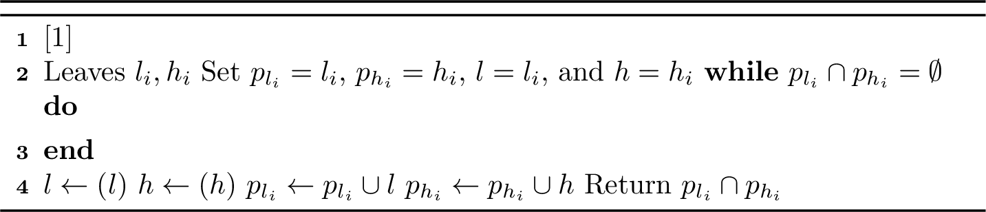
10.4 Insert Query \(\texttt{Insert}(\rho:[x^{(0)}_1:x^{(0)}_2][x^{(1)}_1:x^{(1)}_2])\):↩︎

To insert a region \(\rho= [x^{(0)}_1{:}x^{(0)}_2][x^{(1)}_1{:}x^{(1)}_2]\) chosen by the adversary, we follow a three-step process. First, we insert the horizontal interval \([x^{(0)}_1{:}x^{(0)}_2]\) into \(\mathcal{T}^{(0)}\). Next, we insert the vertical interval \([x^{(1)}_1{:}x^{(1)}_2]\) into the appropriate second-level trees—either regular or lazy structures—associated with nodes \(v_0 \in \mathcal{T}^{(0)}\) whose horizontal range \(\texttt{Int}(v_0)\) intersects \([x^{(0)}_1{:}x^{(0)}_2]\). Finally, we update the auxiliary trees by inserting \([x^{(0)}_1{:}x^{(0)}_2]\) into \(\mathcal{E}^{(0)}\) and \([x^{(1)}_1{:}x^{(1)}_2]\) into \(\mathcal{E}^{(1)}\). We now describe each step in detail.

10.4.0.1 Insertion of the Horizontal Interval \([x^{(0)}_1:x^{(0)}_2]\) :

If the horizontal interval \([x^{(0)}_1{:}x^{(0)}_2]\) does not exist in \(\mathcal{T}^{(0)}\), we insert it using the standard interval tree procedure. Once inserted, we identify the set of nodes \(v_0 \in \mathcal{T}^{(0)}\) whose second-level trees require either regular or lazy insertion of the vertical interval \([x^{(1)}_1{:}x^{(1)}_2]\). These are nodes such that \(\texttt{Int}(v_0)\) intersects or is fully contained by \([x^{(0)}_1{:}x^{(0)}_2]\).

To determine the affected nodes, we locate the leaves \(l_0\) and \(u_0\) containing \(x^{(0)}_1\) and \(x^{(0)}_2\), and define the paths \(p_{l_0}\), \(p_{u_0}\), and \(p_{v_{l_0,u_0}}\) as before, where \(v_{l_0,u_0} = \texttt{First\_Common\_Ancestor}(l_0, u_0)\). We then identify the nodes along these paths for which \([x^{(1)}_1{:}x^{(1)}_2]\) should be regularly or lazily inserted, as detailed in the following subsections.

10.4.0.2 Regular Insertion of the Vertical Interval \([x^{(1)}_1:x^{(1)}_2]\):

As discussed earlier, regular insertion of the vertical interval \([x^{(1)}_1:x^{(1)}_2]\) is required for all nodes \(v_0 \in \mathcal{T}^{(0)}\) such that \(\texttt{Int}(v_0)\) intersects but is not fully contained by \([x^{(0)}_1:x^{(0)}_2]\). These nodes lie along the union of paths \(p_{l_0} \cup p_{u_0}\).

Thus, we traverse each of these paths bottom-up and insert \([x^{(1)}_1:x^{(1)}_2]\) with its corresponding \(\text{reward function parameters}\) \(f_t(\rho_{1,t})\) into the regular second-level trees \(\mathcal{T}^{(1)}_{v_0}\). This insertion follows the standard interval tree procedure used for horizontal intervals.

10.4.0.3 Lazy Insertion of the Vertical Interval \([x^{(1)}_1:x^{(1)}_2]\):

By definition, lazy insertion of the vertical interval \([x^{(1)}_1:x^{(1)}_2]\) applies to nodes \(v_0 \in (p_{l_0} \cup p_{u_0}) \setminus p_{v_{l_0,u_0}}\) whose child subtrees are fully contained by the horizontal interval \([x^{(0)}_1:x^{(0)}_2]\). Specifically:

• For \(v_0 \in p_{l_0}\setminus p_{v_{l_0,u_0}}\): If \(\texttt{Int}(\texttt{Left\_child}(v_0))\) is fully contained by \([x^{(0)}_1:x^{(0)}_2]\), we lazily insert \([x^{(1)}_1:x^{(1)}_2]\) into \(\mathcal{L}^{(1)}_{v_0}\),

• For \(v_0 \in p_{u_0}\setminus p_{v_{l_0,u_0}}\):If \(\texttt{Int}(\texttt{Right\_child}(v_0))\) is fully contained by \([x^{(0)}_1:x^{(0)}_2]\), we insert it into \(\mathcal{R}^{(1)}_{v_0}\).

To perform the insertion, we traverse the nodes in \((p_{l_0} \cup p_{u_0}) \setminus p_{v_{l_0,u_0}}\) bottom-up and apply the standard interval tree insertion routine to each lazy structure. These insertions defer updates to the affected subtrees, preserving efficiency while ensuring that the contributions from \([x^{(1)}_1:x^{(1)}_2]\) are later applied via scaling during queries.

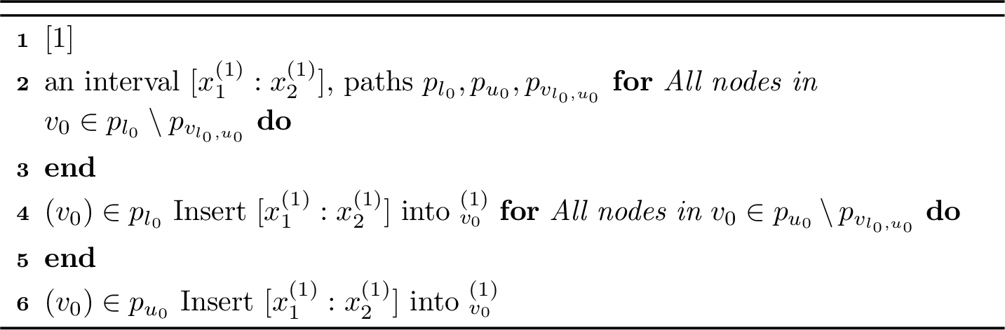
10.4.0.4 Update \(\mathcal{T}\) with \(f_t(\rho)\):

Once the horizontal interval of \(\rho\) is inserted and its vertical interval is lazily or regularly inserted into the appropriate second-level trees, we invoke the \(\texttt{Update}(\rho)\) query. This step aggregates the associated \(\text{reward function parameters}\) of \(\rho\) into all second-level structures where its vertical interval resides, updating the cumulative profile from \(F_{t-1}\) to \(F_t\). This ensures that the drawing algorithm samples actions correctly and that both lazy and regular insertions reflect the contribution of \(f_t(\rho)\).

10.5 Update Query \(\texttt{Update}(\rho:[x^{(0)}_1:x^{(0)}_2][x^{(1)}_1:x^{(1)}_2])\):↩︎

This query updates the data structure by incorporating the \(\text{reward function parameters}\) value \(f_t(\rho)\) of the inserted region \(\rho\) into the existing structure that currently maintains \(F_{t-1}\), thereby producing \(F_t\). To perform this update, we modify the second-level interval trees \(\mathcal{T}^{(1)}_{v_0}\), \(\mathcal{L}^{(1)}_{v_0}\), and \(\mathcal{R}^{(1)}_{v_0}\) associated with the nodes \(v_0 \in \mathcal{T}^{(0)}\), ensuring that the vertical interval \([x^{(1)}_1:x^{(1)}_2]\) of the region \(\rho\) is incorporated into one of these second-level structures.

This update follows standard regular and lazy weight update techniques for interval trees (see [13]), which we adapt to our vector-valued cumulative rewards as regular and lazy \(\text{reward function parameters}\) updates. The lazy \(\text{reward function parameters}\) updates are distinct from lazy insertions. While lazy insertions are used to insert new intervals, lazy \(\text{reward function parameters}\) updates are specifically employed to update the cumulative reward vectors in the second-level trees. Although the routine for handling lazy \(\text{reward function parameters}\) updates remains consistent across all second-level data structures—whether lazy or regular insertion trees—the updates are applied only to the second-level structures of the affected nodes \(v_0 \in \mathcal{T}^{(0)}\) that are impacted by the insertion of \(\rho\).

Although the update process is mostly similar in both lazy and regular insertion data structures, there are minor differences when updating the cumulative reward vectors in each. For simplicity, we describe the process for the regular insertion data structure \(\mathcal{T}^{(1)}_{v_0}\); however, we also highlight the differences with the lazy insertion data structures \(\mathcal{L}^{(1)}_{v_0}\) and \(\mathcal{R}^{(1)}_{v_0}\) as we go through.

10.5.0.1 Locate a Node \(v_0 \in \mathcal{T}\) with Affected \(\mathcal{T}^{(1)}_{v_0}\):

We locate the leaves \(l_0\) and \(u_0\) in \(\mathcal{T}^{(0)}\) whose horizontal ranges \(\texttt{Int}(l_0)\) and \(\texttt{Int}(u_0)\) have \(x^{(0)}_1\) and \(x^{(0)}_2\) as their left and right endpoints, respectively. Let \(p_{l_0}\) and \(p_{u_0}\) denote their respective paths to the root, and let \(v_{l_0,u_0} = \texttt{First\_Common\_Ancestor}(l_0, u_0)\) be their first common ancestor, with path \(p_{v_{l_0,u_0}}\) to the root.

We now update all second-level trees corresponding to nodes along \(p_{l_0}\), \(p_{u_0}\), and \(p_{v_{l_0,u_0}}\) where the vertical interval \([x^{(1)}_1:x^{(1)}_2]\) has been inserted. For each such node \(v_0 \in p_{l_0} \cup p_{u_0}\), we apply the update procedure to its associated \(\mathcal{T}^{(1)}_{v_0}\) as follows:

10.5.0.2 Locate the Vertical Interval \([x^{(1)}_1:x^{(1)}_2]\) in \(\mathcal{T}^{(1)}_{v_0}\):

At this stage, we locate the vertical interval \([x^{(1)}_1:x^{(1)}_2]\) within the relevant second-level tree \(\mathcal{T}^{(1)}_{v_0}\). Let \(l_1\) and \(u_1\) be the leaves containing the left and right endpoints, and let \(p_{l_1}\), \(p_{u_1}\), and \(p_{v_{l_1,u_1}}\) denote the paths from these leaves and their first common ancestor \(v_{l_1,u_1} = \texttt{First\_Common\_Ancestor}(l_1, u_1)\) to the root, respectively.

10.5.0.3 Regular Reward Function Parameters Update in \(\mathcal{T}^{(1)}_{v_0},\) \(\mathcal{L}^{(1)}_{v_0},\) and \(\mathcal{R}^{(1)}_{v_0}\):

We update the cumulative reward vectors \(\vec{r}_{v_0,v_1}\) for all \(v_1 \in p_{l_1} \cup p_{u_1}\) using the following update rule: \[\begin{align} \vec{r}_{v_0,v_1} &\leftarrow \vec{r}_{v_0,v_1} + \vec{A}_{\rho'}, \label{alg:lupdl39} \end{align}\tag{14}\] where \(\rho' = [\texttt{Int}(v_0) \cap [x^{(0)}_1:x^{(0)}_2]][\texttt{Int}(v_1) \cap [x^{(1)}_1:x^{(1)}_2]]\), and \(\vec{A}_{\rho'}\) is computed by integrating the mapping function \(g\) over \(\rho'\) with coefficient vector \(f_t(\rho)\), as described in Section 7.1.

In contrast, for the lazy insertion structures \(\mathcal{L}^{(1)}_{v_0}\) and \(\mathcal{R}^{(1)}_{v_0}\) for the nodes \(w_1 \in p_{l_1} \cup p_{u_1} \setminus p_{v_{l_1,u_1}}\), which defer updates to be scaled down during queries, the update is performed as follows: \[\begin{align} \vec{r}_{v_0,w_1} &\leftarrow \vec{r}_{v_0,w_1} + \vec{A}_{\rho''}, \label{alg:lupdl391} \end{align}\tag{15}\] where \(\rho'' = [\texttt{Int}(v_0)][\texttt{Int}(w_1) \cap [x^{(1)}_1:x^{(1)}_2]]\) spans the full horizontal range of the subtree rooted at \(v_0\). To simplify the scaling process when the lazy insertion structures are later accessed during query time, we treat the range \(\texttt{Int}(v_0)\) as fully contained by the horizontal interval \([x^{(0)}_1:x^{(0)}_2]\). This treatment facilitates the downward scaling of updates into the subtrees, ensuring that the update remains compatible with the information stored in \(\mathcal{T}^{(1)}_{v_0}\), without affecting the correctness of the algorithm.

10.5.0.4 Lazy Reward Function Parameters Update in \(\mathcal{T}^{(1)}_{v_0}\), \(\mathcal{L}^{(1)}_{v_0}\), and \(\mathcal{R}^{(1)}_{v_0}\):

The lazy \(\text{reward function parameters}\) update proceeds by traversing the paths \(p_{l_1} \setminus p_{v_{l_1,u_1}}\) and \(p_{u_1} \setminus p_{v_{l_1,u_1}}\) in a bottom-up manner. At each node \(v_1\) along these paths, a lazy update message, either \(\texttt{Lazy\_Update\_Message}_{v_1, \texttt{Right\_child}(v_1)}\) or \(\texttt{Lazy\_Update\_Message}_{v_1, \texttt{Left\_child}(v_1)}\), is sent to the child whose vertical interval is strictly contained in \([x^{(1)}_1:x^{(1)}_2]\). In this context, \(\texttt{Lazy\_Update\_Message}_{v'_0,v'_1}\) represents the lazy \(\text{reward function parameters}\) update message sent by node \(\texttt{Par}(v'_1)\) to its child \(v'_1\) in the second-level \(\texttt{Interval Tree}\) associated with \(v'_0 \in \mathcal{T}^{(0)}\). Each lazy update message carries a cumulative \(\text{reward function parameters}\) vector that has not yet been propagated. Since these vectors are intended to uniformly influence the entire subtree rooted at the recipient, they are aggregated and integrated during propagation. The final aggregated results are then applied during query-time integration.

We begin with the nodes \(v_1\) along the path \(p_{l_1} \setminus p_{v_{l_1,u_1}}\). If the left child \(\texttt{Left\_child}(v_1)\) lies on the path, we send a lazy \(\text{reward function parameters}\) update message to the right child \(\texttt{Right\_child}(v_1)\) as follows: \[\begin{align} \texttt{Lazy\_Update\_Message}_{v_0,\texttt{Right\_child}(v_1)} &\leftarrow \texttt{Lazy\_Update\_Message}_{v_0,\texttt{Right\_child}(v_1)} + f_t(\rho). \label{alg:lupd2} \end{align}\tag{16}\]

Next, we apply the same update process to the nodes \(v_1 \in p_{u_1} \setminus p_{v_{l_1,u_1}}\), with a slight variation. If the right child \(\texttt{Right\_child}(v_1)\) also belongs to the path \(p_{u_1} \setminus p_{v_{l_1,u_1}}\), we send a lazy update message to the left child \(\texttt{Left\_child}(v_1)\), as follows: \[\begin{align} \texttt{Lazy\_Update\_Message}_{v_0,\texttt{Left\_child}(v_1)} &\leftarrow \texttt{Lazy\_Update\_Message}_{v_0,\texttt{Left\_child}(v_1)} + f_t(\rho). \label{alg:lupd3} \end{align}\tag{17}\]

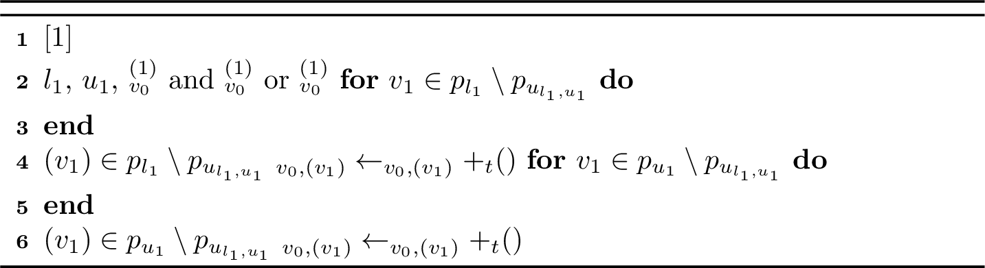
10.5.0.5 Lazy Reward Function Update Messages Propagation

We now describe how lazy \(\text{reward function parameters}\) update messages are propagated and cleared in both regular and lazy insertion data structures. These propagations are triggered during insertions, updates, or query operations (e.g., a \(\texttt{Draw}\) query), typically when locating a leaf. For such operations, the algorithm identifies the relevant leaves \(l_1\) and \(u_1\) in \(\mathcal{T}^{(1)}_{v_0}\), and applies any pending lazy update messages ( \(\texttt{Lazy\_Update\_Message}\) ) along the corresponding root-to-leaf paths, \(p_{l_1}\) or \(p_{u_1}\).

The mechanism is uniform across both the regular insertion structure \(\mathcal{T}^{(1)}_{v_0}\) and the lazy insertion structures \(\mathcal{L}^{(1)}_{v_0}\) and \(\mathcal{R}^{(1)}_{v_0}\). In all cases, the algorithm traverses the path top-down and applies the lazy messages just before descending to a child.

For instance, consider the downward traversal of \(p_{l_1}\), starting from \(v_1 = \texttt{Root}(\mathcal{T}^{(1)}_{v_0})\). Before descending to the right child \(\texttt{Right\_child}(v_1)\), the algorithm updates the corresponding cumulative reward vector as: \[\begin{align} \vec{r}_{v_0,\texttt{Right\_child}(v_1)} \leftarrow \vec{r}_{v_0,\texttt{Right\_child}(v_1)} + \vec{A}_{\rho'}, \label{eq:lz1} \end{align}\tag{18}\] where \(\rho' :[\texttt{Int}(v_0)][\texttt{Int}(\texttt{Right\_child}(v_1))]\) in both the regular and lazy insertion structures. The coefficient vector used to compute \(\vec{A}_{\rho'}\) is \(\texttt{Lazy\_Update\_Message}_{v_0,\texttt{Right\_child}(v_1)}\). This guarantees that deferred updates are consistently applied and that contributions remain correctly scaled.

Then, as the algorithm proceeds to the child \(\texttt{Right\_child}(v_1)\), it pushes the lazy message further down to both its children. Let \(v'_1 = \texttt{Left\_child}(\texttt{Right\_child}(v_1))\) and \(v''_1 = \texttt{Right\_child}(\texttt{Right\_child}(v_1))\). The propagation is done by: \[\begin{align} \texttt{Lazy\_Update\_Message}_{v_0,v'_1} &\leftarrow \texttt{Lazy\_Update\_Message}_{v_0,v'_1} + \texttt{Lazy\_Update\_Message}_{v_0,\texttt{Right\_child}(v_1)}, \tag{19} \\ \texttt{Lazy\_Update\_Message}_{v_0,v''_1} &\leftarrow \texttt{Lazy\_Update\_Message}_{v_0,v''_1} + \texttt{Lazy\_Update\_Message}_{v_0,\texttt{Right\_child}(v_1)}, \tag{20} \end{align}\] and the original message is then cleared: \[\texttt{Lazy\_Update\_Message}_{v_0,\texttt{Right\_child}(v_1)} \leftarrow \vec{0}.\]

The same procedure applies symmetrically if the traversal goes through \(\texttt{Left\_child}(v_1)\). This unified handling across both regular and lazy data structures ensures that all lazy updates are correctly propagated and scaled, maintaining the correctness and efficiency of cumulative reward computations.

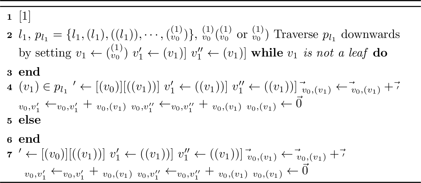
10.6 Cumulative Reward Retrieval Query \(\texttt{CReward}(\rho:[x^{(0)}_1:x^{(0)}_2][x^{(1)}_1:x^{(1)}_2])\)↩︎

This query returns the cumulative rewards associated with a given rectangular region \(\rho\) by aggregating all relevant vectors \(\vec{r}_{v_0,v_1}\) stored across the data structure and map it to the real valued cumulative reward. Specifically, it gathers contributions from nodes \(v_0 \in \mathcal{T}^{(0)}\) and nodes \(v_1\) in the corresponding second-level structures—\(\mathcal{T}^{(1)}_{v_0}\), \(\mathcal{L}^{(1)}_{v_0}\), or \(\mathcal{R}^{(1)}_{v_0}\)—such that:

• the horizontal range \(\texttt{Int}(v_0)\) intersects with or fully contains the horizontal interval \([x^{(0)}_1:x^{(0)}_2]\), and

• the vertical range \(\texttt{Int}(v_1)\) intersects with or fully contains the vertical interval \([x^{(1)}_1:x^{(1)}_2]\).

In our multi-stage drawing algorithm (described in Section 10.7), we work with locating atomic intervals along each coordinate in a sequential manner, following the hierarchy of \(\mathcal{T}\). To clarify the notation, we define atomic intervals as those that are indivisible along their respective coordinates. Specifically, we use primes in the intervals \([x'^{(0)}_1:x'^{(0)}_2]\) and \([x'^{(1)}_1:x'^{(1)}_2]\) to indicate that these intervals are atomic with respect to the corresponding coordinate. Here, \([x'^{(0)}_1:x'^{(0)}_2]\) represents an atomic horizontal interval in the \(x^{(0)}\)-coordinate, and \([x'^{(1)}_1:x'^{(1)}_2]\) represents an atomic vertical interval in the \(x^{(1)}\)-coordinate.

Based on this structure, we divide the cumulative reward retrieval query into two subroutines. The algorithm first locates an atomic horizontal interval \([x'^{(0)}_1:x'^{(0)}_2]\) by querying regions of the form \(\rho' : [x^{(0)}_1:x^{(0)}_2][0:1]\), handled by the subroutine \(\texttt{CReward}^{(0)}(\rho')\). Once the horizontal atomic interval is identified, the algorithm then locates the atomic vertical interval \([x'^{(1)}_1:x'^{(1)}_2]\) by querying over \(\rho'': [x'^{(0)}_1:x'^{(0)}_2][x^{(1)}_1:x^{(1)}_2]\), using the subroutine \(\texttt{CReward}^{(1)}(\rho'')\).

We therefore distinguish between the following two classes of cumulative reward queries:

• \(\texttt{CReward}^{(0)}(\rho')\): queries of the form \([x^{(0)}_1:x^{(0)}_2][0:1]\), which return cumulative rewards over general horizontal intervals and the full vertical range.

• \(\texttt{CReward}^{(1)}(\rho'')\): queries of the form \([x'^{(0)}_1:x'^{(0)}_2][x^{(1)}_1:x^{(1)}_2]\), where the horizontal interval is atomic and the vertical interval may be arbitrary.

Here, \(\texttt{CReward}^{(i)}(\rho)\) retrieves the cumulative reward for a region \(\rho\) where the first \(i-1\) coordinate intervals are atomic and fixed by previous stages, while the \(i\)-th coordinate spans a general interval defined by the endpoints inserted by the adversary. The remaining coordinates correspond to open subspaces, represented by the interval \([0:1]\).

This separation is crucial: for instance, in the two-dimensional case, all horizontal intervals are stored in \(\mathcal{T}^{(0)}\), while vertical intervals are distributed across second-level data structures attached to individual nodes in \(\mathcal{T}^{(0)}\). As a result, once the horizontal interval is fixed, retrieving cumulative rewards for vertical atomic intervals must be handled differently and locally across the second-level structures.

Handling both types of queries involves first identifying the set of second-level data structures \(\mathcal{S}^{(1)}\) in \(\mathcal{T}\) whose stored intervals correspond to all the regions that either intersect with or fully contain the query region \(\rho\). We then retrieve the relevant portions of the cumulative rewards from these structures and aggregate them to compute the total cumulative reward \(r(\rho)\). A crucial requirement for the correctness of this aggregation is that the data structures in \(\mathcal{S}^{(1)}\) store disjoint information with respect to the \(\text{reward function parameters}\) of any region intersecting \(\rho\). In other words, if the vertical intervals stored in these data structures do not share any common endpoints, there will be no region that intersects \(\rho\) and is counted twice. This disjointness ensures that there is no overlap or double-counting when summing the contributions across different subtrees, which follows directly from the recursive and non-overlapping design of the lazy and regular structures in \(\mathcal{T}\).

10.6.1 \(\texttt{CReward}^{(0)}(\rho:[x^{(0)}_1:x^{(0)}_2][0:1])\)↩︎

To process this query, we first identify the leaves \(l_0\) and \(u_0\) in \(\mathcal{T}^{(0)}\) that contain the endpoints of the horizontal interval \([x^{(0)}_1:x^{(0)}_2]\), and compute their first common ancestor \(v_{l_0,u_0}\). Let \(p_{l_0}\), \(p_{u_0}\), and \(p_{v_{l_0,u_0}}\) denote the paths from \(l_0\), \(u_0\), and \(v_{l_0,u_0}\) to the root of \(\mathcal{T}^{(0)}\), respectively.

Since \(\texttt{Int}(v_{l_0,u_0})\) contains \([x^{(0)}_1:x^{(0)}_2]\), we distinguish two cases: either \(\texttt{Int}(v_{l_0,u_0}) = [x^{(0)}_1:x^{(0)}_2]\), or \(\texttt{Int}(v_{l_0,u_0})\) strictly contains the horizontal interval \([x^{(0)}_1:x^{(0)}_2]\).

1. Case \(\texttt{Int}(v_{l_0,u_0}) = [x^{(0)}_1:x^{(0)}_2]\):

   In this case, we aim to retrieve and return the cumulative reward of the region \(\rho\) as \(r([\texttt{Int}(v_{l_0,u_0})][0,1])\). This value consists of two contributing components:

   • The first component is the portion of the cumulative rewards from regions whose horizontal intervals intersect, but do not fully contain, the range \(\texttt{Int}(v_{l_0,u_0})\) maintained at \(v_{l_0,u_0}\). These regions contribute to the cumulative rewards of the region \(\rho\) due to their intersection. By definition, the aggregated cumulative \(\text{reward function parameters}\) vectors of such regions over the region \(\rho: [\texttt{Int}(v_{l_0,u_0})][0,1]\) can be directly retrieved from the root of the regular insertion tree \(\mathcal{T}^{(1)}_{v_{l_0,u_0}}\), which aggregates parts of the cumulative rewards of these regions.

   • The second component is the portion of the cumulative rewards from regions whose horizontal intervals fully contain \(\texttt{Int}(v_{l_0,u_0})\). These regions are stored in the lazy insertion trees \(\mathcal{L}^{(1)}_{v_0}\) and \(\mathcal{R}^{(1)}_{v_0}\) for all nodes \(v_0\) along the path \(p_{v_{l_0,u_0}}\), i.e., ancestors of \(v_{l_0,u_0}\). If \(v_{l_0,u_0}\) is in the left (resp.right) subtree of \(v_0\), we retrieve the relevant data from \(\mathcal{L}^{(1)}_{v_0}\) (resp.\(\mathcal{R}^{(1)}_{v_0}\)) and apply the appropriate scaling.

   We then collect all the second-level data structures into a set \(\mathcal{S}^{(1)}\), as previously mentioned, and query each structure to retrieve the corresponding part of the cumulative reward for the region \(\rho\). To formalize this process, we define the set \(\mathcal{S}^{(1)}_{v_{l_0,u_0}}\) to include all second-level structures relevant for computing the cumulative reward \(r(\rho)\). Initially, this set contains the regular insertion tree associated with \(v_{l_0,u_0}\):

   \[\mathcal{S}^{(1)}_{v_{l_0,u_0}} \gets \left\{ \mathcal{T}^{(1)}_{v_{l_0,u_0}} \right\}.\] We then traverse the path \(v_0 \in p_{v_{l_0,u_0}}\) and augment this set as follows: \[\begin{align} \mathcal{S}^{(1)}_{v_{l_0,u_0}} &\gets \mathcal{S}^{(1)}_{v_{l_0,u_0}} \cup \mathcal{L}^{(1)}_{v_0} \quad \text{if } \texttt{Left\_child}(v_0) \in p_{v_{l_0,u_0}},\\ \mathcal{S}^{(1)}_{v_{l_0,u_0}} &\gets \mathcal{S}^{(1)}_{v_{l_0,u_0}} \cup \mathcal{R}^{(1)}_{v_0} \quad \text{if } \texttt{Right\_child}(v_0) \in p_{v_{l_0,u_0}}. \end{align}\]

   

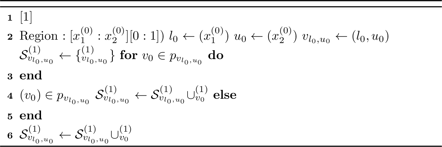
   We index the second-level data structures in the set \(\mathcal{S}^{(1)}_{v_{l_0,u_0}}\) by \(S^{(1)}_{v_0}\), where each structure corresponds to the second-level data associated with the node \(v_0 \in p_{v_{l_0,u_0}}\) and is inserted into \(\mathcal{S}^{(1)}_{v_{l_0,u_0}}\). In particular, the only regular insertion second-level tree in this set, \(\mathcal{T}^{(1)}_{v_{l_0,u_0}}\), is responsible for regions whose horizontal intervals intersect with, but do not fully contain, the horizontal interval \(\texttt{Int}(v_{l_0,u_0})\) of the region \(\rho\). The remaining second-level data structures in \(\mathcal{S}^{(1)}_{v_{l_0,u_0}}\) are lazy insertion trees associated with ancestor nodes \(v_0\) for which \(\texttt{Int}(v_0)\) fully contains \(\texttt{Int}(v_{l_0,u_0})\). In summary, \(S^{(1)}_{v_{l_0,u_0}} = \mathcal{T}^{(1)}_{v_{l_0,u_0}}\) and the rest are lazy structures. Thus, the cumulative reward for \(\rho\) is given by:

   \[\begin{align} \texttt{CReward}^{(0)}(\rho) = \underbrace{r_{S^{(1)}_{v_{l_0,u_0}}}(\rho)}_{\text{cumulative rewards of the regular insertion tree}} + \underbrace{\sum_{S^{(1)}_{v_0}\in \mathcal{S}^{(1)}_{v_{l_0,u_0}}\setminus S^{(1)}_{v_{l_0,u_0}}} r_{S^{(1)}_{v_0}}(\rho)}_{\text{cumulative rewards of the lazy insertion trees}}, \label{crew:detach} \end{align}\tag{21}\]

   where \(r_{S^{(1)}_{v_0}}(\rho)\) represents the cumulative reward of the region \(\rho\) with respect to the regions whose intervals are stored in the data structure \(S^{(1)}_{v_0}\).

   For each term of the equation 21 , we retrieve the cumulative reward vectors from each data structure, apply scaling where needed, and aggregate the results to return \(r(\rho:[\texttt{Int}(v_{l_0,u_0})][0:1])\). For the regular insertion tree \(S^{(1)}_{v_{l_0,u_0}}\) in \(\mathcal{S}^{(1)}_{v_{l_0,u_0}}\), we retrieve the vectors without scaling, as they are computed by integrating over regions with the appropriate range on the first coordinate. For the lazy insertion trees in \(\mathcal{S}^{(1)}_{v_{l_0,u_0}}\), we scale each cumulative reward vector to the region \(\rho= [\texttt{Int}(v_{l_0,u_0})][0:1]\), which is a subregion of \([\texttt{Int}(v_0)][0:1]\).

   To compute the first term of equation 21 , which is directly accessible from the cumulative reward vector stored at the root of the regular insertion tree \(S^{(1)}_{v_{l_0,u_0}}\), we have: \[\begin{align} r_{S^{(1)}_{v_{l_0,u_0}}}(\rho) = \sum_{j \in [A]} \vec{r}^{(j)}_{v_{l_0,u_0},\texttt{Root}(S^{(1)}_{v_0})},\label{crew:detach1} \end{align}\tag{22}\] where \(A\) is the number of basis monomials in the mapping function \(g\), and \(\alpha^j_i\) is the exponent of the \(i\)-th coordinate variable in the \(j\)-th monomial. The term \(\vec{r}^{(j)}_{v_{l_0,u_0},\texttt{Root}(S^{(1)}_{v_0})}\) represents the \(j\)-th entry of the cumulative reward vector. These basis terms are fixed and detailed in Section 7.1.

   For the lazy data structures appearing in the second term of equation 21 , we follow the same procedure as for the regular insertion trees. However, as previously mentioned, the scaling procedure is particularly important for the cumulative reward vectors at the roots of these data structures, such as \(\vec{r}_{v_0,\texttt{Root}(S^{(1)}_{v_0})}\), since these vectors are computed over regions with a horizontal interval equal to \(\texttt{Int}(v_0)\). We iterate over each data structure \(S^{(1)}_{v_0} \in \mathcal{S}^{(1)}_{v_{l_0,u_0}} \setminus S^{(1)}_{v_{l_0,u_0}}\), extract the cumulative reward vector at the root \(\vec{r}_{v_0,\texttt{Root}(S^{(1)}_{v_0})}\), and scale it to \(\rho\). Let \(\texttt{Int}(v_0) = [a^{(0)}_1:a^{(0)}_2]\), \(\texttt{Int}(\texttt{Root}(S^{(1)}_{v_0})) = [a^{(1)}_1 = 0 : a^{(1)}_2 = 1]\), and \(\texttt{Int}(v_{l_0,u_0}) = [x^{(0)}_1:x^{(0)}_2]\), with \([x^{(1)}_1 = 0 : x^{(1)}_2 = 1]\). We then apply the scaling rule from Equation 4 , yielding:

   \[\begin{align} \label{crew:detach2} \end{align}\tag{23}\] where \(A\) is the number of basis monomials in the mapping function \(g\), and \(\alpha^j_i\) is the exponent of the \(i\)-th coordinate variable in the \(j\)-th monomial. The term \(\vec{r}^{(j)}_{v_0,\texttt{Root}(S^{(1)}_{v_0})}\) represents the \(j\)-th entry of the cumulative reward vector. These basis terms are fixed and detailed in Section 7.1.

   Finally we would have, \[\begin{align} \texttt{CReward}^{(0)}(\rho) = \text{\eqref{crew:detach1}} + \text{\eqref{crew:detach2}}. \end{align}\]

2. Case \([x^{(0)}_1:x^{(0)}_2] \subset\texttt{Int}(v_{l_0,u_0})\):

   For the second case, where \([x^{(0)}_1:x^{(0)}_2] \subset \texttt{Int}(v_{l_0,u_0})\), we begin by computing \(r([\texttt{Int}(v_{l_0,u_0})][0:1])\) using the method described for the exact-match case via the query \(\texttt{CReward}^{(0)}([\texttt{Int}(v_{l_0,u_0})][0:1])\). We then refine this result by subtracting contributions from subregions outside \([x^{(0)}_1:x^{(0)}_2]\) but still within \(\texttt{Int}(v_{l_0,u_0})\).

   To do this, we traverse the paths \(p_{l_0} \setminus p_{v_{l_0,u_0}}\) and \(p_{u_0} \setminus p_{v_{l_0,u_0}}\) in a bottom-up manner and prune subtrees that fall entirely outside the query interval. Specifically, for each \(v'_0 \in p_{l_0} \setminus p_{v_{l_0,u_0}}\), if \(\texttt{Left\_child}(v'_0)\) is not on the path, we subtract \(r([\texttt{Int}(\texttt{Left\_child}(v'_0))][0:1])\). Similarly, for each \(v''_0 \in p_{u_0} \setminus p_{v_{l_0,u_0}}\), if \(\texttt{Right\_child}(v''_0)\) is not on the path, we subtract \(r([\texttt{Int}(\texttt{Right\_child}(v''_0))][0:1])\). These values are computed recursively using \(\texttt{CReward}^{(0)}(\cdot)\), ensuring modularity and correctness.

   This pruning ensures that the final result corresponds exactly to the cumulative reward over \([x^{(0)}_1:x^{(0)}_2][0:1]\), excluding any contributions from outside this interval.

   

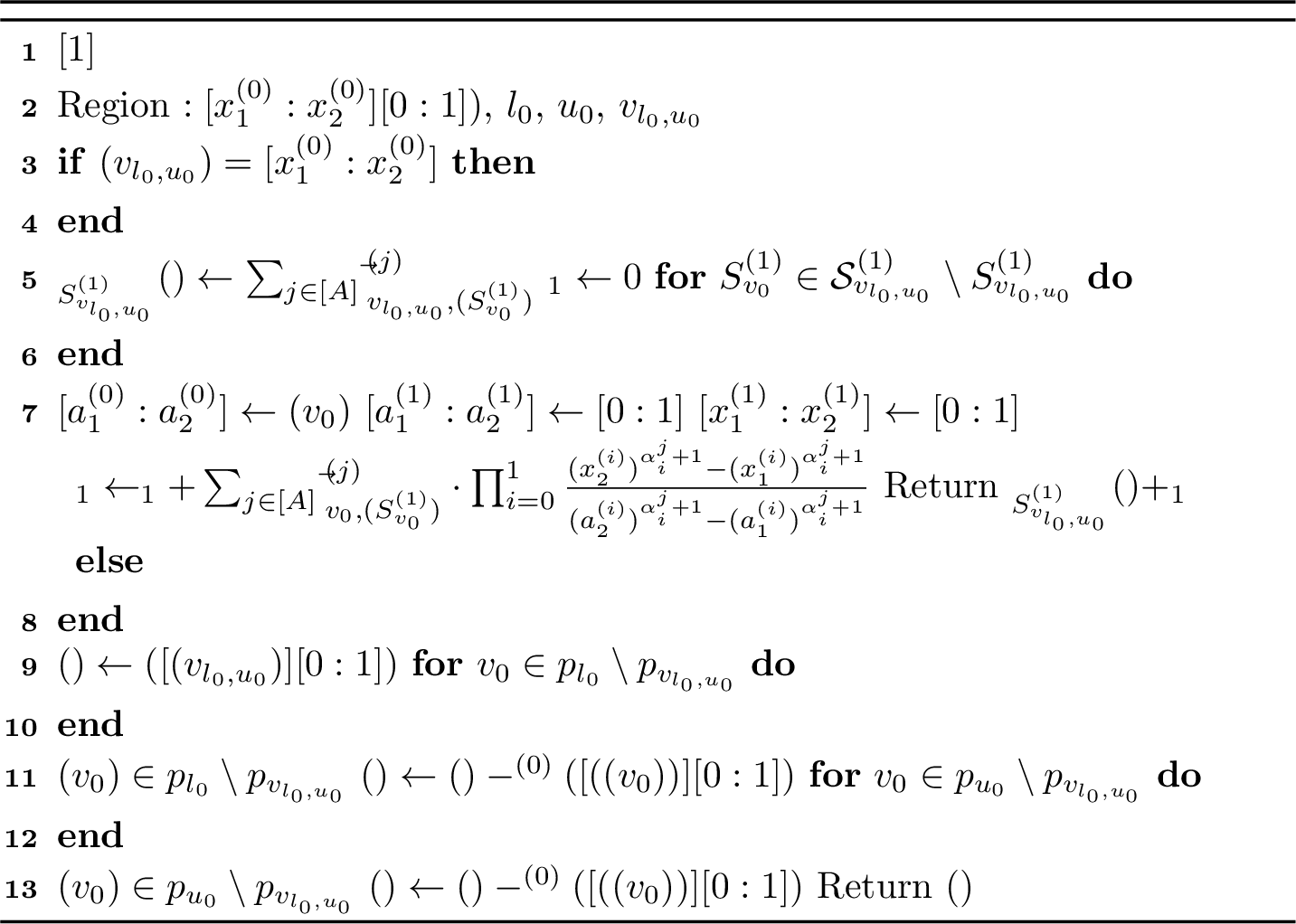
10.6.2 \(\texttt{CReward}^{(1)}\left(\rho:[x'^{(0)}_1:x'^{(0)}_2][x^{(1)}_1:x^{(1)}_2]\right)\)↩︎

Given the definition of \(\texttt{CReward}^{(1)}\), assume the horizontal interval \([x'^{(0)}_1:x'^{(0)}_2]\) is atomic and corresponds to a leaf \(l_0 \in \mathcal{T}^{(0)}\), i.e., \(\texttt{Int}(l_0) = [x'^{(0)}_1:x'^{(0)}_2]\). Let \(p_{l_0}\) denote the path from \(l_0\) to the root. To compute \(\texttt{CReward}^{(1)}(\rho)\), we collect all second-level data structures that affect \(\texttt{Int}(l_0)\) into the set \(\mathcal{S}^{(1)}_{l_0}\), following the same method as for \(\texttt{CReward}^{(0)}\). We similarly would have all data structures in \(\mathcal{S}^{(1)}_{l_0}\) to be lazy insertion data structures except \(S^{(1)}_{l_0}\), which is \(\mathcal{T}^{(1)}_{l_0}\). Thus, similar to equation 21 , we can write:

\[\begin{align} \texttt{CReward}^{(1)}(\rho) = \underbrace{r_{S^{(1)}_{l_0}}(\rho)}_{\text{cumulative rewards of the regular insertion tree}} + \underbrace{\sum_{S^{(1)}_{v_0} \in \mathcal{S}^{(1)}_{l_0} \setminus S^{(1)}_{l_0}} r_{S^{(1)}_{v_0}}(\rho)}_{\text{cumulative rewards of the lazy insertion trees}}, \label{crew:detachplus} \end{align}\tag{24}\]

For the first term of equation 24 , we retrieve \(r_{S^{(1)}_{l_0}}(\rho)\) from the data structure \(S^{(1)}_{l_0}\) without scaling. Then, we traverse the remaining lazy insertion data structures in \(\mathcal{S}^{(1)}_{l_0}\), retrieve the cumulative reward vectors for the region \(\rho':[\texttt{Int}(v_0)][x^{(1)}_1:x^{(1)}_2]\) in each \(S^{(1)}_{v_0} \in \mathcal{S}^{(1)}_{l_0}\), and scale them to \(\rho\). Although the cumulative rewards are retrieved for regions with similar vertical intervals in each \(S^{(1)}_{v_0}\), the disjointness of the data structures in \(\mathcal{S}^{(1)}_{l_0}\) prevents double-counting, ensuring accurate aggregation.

The main distinction from the previous subclass of queries is that the cumulative reward vectors specifying the vertical interval \([x^{(1)}_1:x^{(1)}_2]\) are not necessarily stored at the root of the data structures in \(\mathcal{S}^{(1)}_{l_0}\). Additionally, the way vertical intervals are maintained in the second-level data structures introduces another challenge. Specifically, the vertical interval endpoints are not stored within a single \(\texttt{Interval Tree}\); rather, they are distributed across different data structures associated with various nodes in \(\mathcal{T}^{(0)}\). To clarify, when handling queries of the form \(\texttt{CReward}^{(0)}(\cdot)\), we assume the vertical interval of the queried region is \([0:1]\), which is guaranteed to be stored at the root of each data structure. However, in this subclass of queries, it is not guaranteed that there exists a leaf whose range exactly matches \([x^{(1)}_1:x^{(1)}_2]\). As a result, when locating the endpoints of \([x^{(1)}_1:x^{(1)}_2]\) in each data structure, we may end up at a leaf where neither endpoint corresponds to \(x^{(1)}_1\) or \(x^{(1)}_2\). We detail the process in the following section.

We first identify the leaves \(l_1\) and \(u_1\) in \(S^{(1)}_{v_0}\), where \(v_0 \in p_{l_0}\), that contain \(x^{(1)}_1\) and \(x^{(1)}_2\), respectively. Let \(\texttt{Int}(l_1) = [a_1^{(1)}:a_2^{(1)}]\) and \(\texttt{Int}(u_1) = [b_1^{(1)}:b_2^{(1)}]\), and define their first common ancestor \(v_{l_1,u_1}\) such that \([a_1^{(1)}:b_2^{(1)}] \subseteq \texttt{Int}(v_{l_1,u_1})\).

For a given data structure \(S^{(1)}_{v_0}\), which can be either a regular or lazy insertion tree, if both endpoints of the vertical interval \([x^{(1)}_1:x^{(1)}_2]\) are stored in \(S^{(1)}_{v_0}\), then \(a^{(1)}_1 = x^{(1)}_1\) and \(b^{(1)}_2 = x^{(1)}_2\). In this case, for both the first and second terms of equation 24 , to compute \(r_{S^{(1)}_{l_0}}(\rho)\), we first retrieve the cumulative reward for \(\rho' = [\texttt{Int}(v_0)][a^{(1)}_1:b^{(1)}_2]\) in the same way as the \(\texttt{CReward}^{(0)}\) case. This involves retrieving the cumulative reward over the larger region \(\rho'' = [\texttt{Int}(v_0)][\texttt{Int}(v_{l_1,u_1})]\), pruning the excess contributions outside \([\texttt{Int}(v_0)][a^{(1)}_1:b^{(1)}_2]\), and scaling the result over \(\texttt{Int}(l_0) = [x'^{(0)}_1:x'^{(0)}_2]\) to match the target region \([\texttt{Int}(l_0)][a^{(1)}_1:b^{(1)}_2]\).

As noted earlier, unlike \(\mathcal{T}^{(0)}\), \(S^{(1)}_{v_0}\) does not store all the endpoints of the vertical intervals. Therefore, pruning the unnecessary portions of \(\rho'' = [\texttt{Int}(v_0)][\texttt{Int}(v_{l_1,u_1})]\) requires handling partial coverage at the boundaries, specifically at \(\texttt{Int}(l_1)\) and \(\texttt{Int}(u_1)\). If \(x^{(1)}_1\) is not stored in \(S^{(1)}_{v_0}\), then \(a^{(1)}_1 < x^{(1)}_1 < a^{(1)}_2\), and similarly, if \(x^{(1)}_2\) is missing from \(S^{(1)}_{v_0}\), then \(b^{(1)}_1 < x^{(1)}_2 < b^{(1)}_2\). In these cases, we exclude \(r_{S^{(1)}_{v_0}}([\texttt{Int}(v_0)][a^{(1)}_1:x^{(1)}_1])\) and \(r_{S^{(1)}_{v_0}}([\texttt{Int}(v_0)][x^{(1)}_2:b^{(1)}_2])\) from \(r_{S^{(1)}_{v_0}}(\rho')\). While handling boundaries for both lazy and regular data structures is largely similar, a scaling step is necessary when handling boundaries in lazy data structures, i.e., in \(\mathcal{S}^{(1)}_{l_0} \setminus S^{(1)}_{l_0}\). We detail both cases below.

1. Compute \(r_{S^{(1)}_{l_0}}(\rho)\):

   For the regular insertion data structure in the first term of equation 24 , the cumulative reward retrieval for the region \(\rho\), denoted \(r_{S^{(1)}_{l_0}}(\rho)\), is computed as follows:

   \[\begin{align} r_{S^{(1)}_{l_0}}(\rho) = r_{S^{(1)}_{l_0}}(\rho') - u_{l_1} - u_{u_1}, \label{crew1:reg} \end{align}\tag{25}\] where \(\rho' = [\texttt{Int}(l_0)][a^{(1)}_1:b^{(1)}_2]\) is the region from which the cumulative reward is computed. Specifically, \(u_{l_1} = r_{S^{(1)}_{l_0}}([\texttt{Int}(l_0)][a^{(1)}_1:x^{(1)}_1])\) and \(u_{u_1} = r_{S^{(1)}_{l_0}}([\texttt{Int}(l_0)][x^{(1)}_2:b^{(1)}_2])\) represent the cumulative rewards of the excess contributions from the leaves \(l_1\) and \(u_1\), which must be excluded.

   To compute \(u_{l_1}\) and \(u_{u_1}\), we exploit the fact that \(l_0\), \(l_1\), and \(u_1\) are all leaves, and the regions \([\texttt{Int}(l_0)][\texttt{Int}(l_1)]\) and \([\texttt{Int}(l_0)][\texttt{Int}(u_1)]\) are atomic regions. Thus, the cumulative \(\text{reward function parameters}\) vectors \(\vec{r}_{l_0,l_1}\) and \(\vec{r}_{l_0,u_1}\) can be scaled over the second coordinate to accurately compute \(u_{l_1} = r_{S^{(1)}_{l_0}}([\texttt{Int}(l_0)][a^{(1)}_1:x^{(1)}_1])\) and \(u_{u_1} = r_{S^{(1)}_{l_0}}([\texttt{Int}(l_0)][x^{(1)}_2:b^{(1)}_2])\), as follows:

   We compute the excess contribution from the lower boundary by scaling the vector \(\vec{r}_{l_0,l_1}\) to the region \([\texttt{Int}(l_0)][a^{(1)}_1:x^{(1)}_1]\). The resulting contribution is given by:

   \[\begin{align} u_{l_1} = \sum_{j \in [A]} \vec{r}^{(j)}_{l_0,l_1} \cdot \frac{(x^{(1)}_1)^{\alpha^j_1 + 1} - (a^{(1)}_1)^{\alpha^j_1 + 1}}{(a^{(1)}_2)^{\alpha^j_1 + 1} - (a^{(1)}_1)^{\alpha^j_1 + 1}}, \label{crew1:reg1} \end{align}\tag{26}\]

   where no scaling is applied to the first coordinate because \(l_0\) is a leaf, and its regular insertion tree \(S^{(1)}_{l_0} = \mathcal{T}^{(1)}_{l_0}\) contains the \(\text{reward function parameters}\) values of regions whose horizontal intervals contain \(\texttt{Int}(l_0)\). Therefore, the integration within this tree is performed over the entire \(\texttt{Int}(l_0)\), and no scaling is necessary for that coordinate.

   Similarly, the contribution from the upper boundary is computed by scaling the vector \(\vec{r}_{v_0,u_1}\) to the region \([\texttt{Int}(l_0)][x^{(1)}_2:b^{(1)}_2]\), as:

   \[\begin{align} u_{u_1} = \sum_{j \in [A]} \vec{r}^{(j)}_{l_0,u_1} \cdot \frac{(b^{(1)}_2)^{\alpha^j_1 + 1} - (x^{(1)}_2)^{\alpha^j_1 + 1}}{(b^{(1)}_2)^{\alpha^j_1 + 1} - (b^{(1)}_1)^{\alpha^j_1 + 1}}. \label{crew1:reg2} \end{align}\tag{27}\]

   According to 25 , subtracting \(u_{l_1} + u_{u_1}\) from the full-interval contribution \(r_{S^{(1)}_{l_0}}([\texttt{Int}(l_0)][a^{(1)}_1:b^{(1)}_2])\), and applying the vertical scaling step, yields the desired cumulative reward \(r_{S^{(1)}_{l_0}}\) for the region \([x'^{(0)}_1:x'^{(0)}_2][x^{(1)}_1:x^{(1)}_2]\).

2. Computing \(\sum_{S^{(1)}_{v_0} \in \mathcal{S}^{(1)}_{l_0} \setminus S^{(1)}_{l_0}} r_{S^{(1)}_{v_0}}(\rho)\):

   To retrieve the cumulative reward for the region \(\rho\) in each lazy insertion data structure \(S^{(1)}_{v_0} \in \mathcal{S}^{(1)}_{l_0}\), we apply the same procedure as for the regular data structure \(S^{(1)}_{l_0}\). However, there is a slight difference in the scaling step because the horizontal range of the nodes \(\texttt{Int}(v_0) = [x''^{(0)}_1:x''^{(0)}_2]\) does not match \(\texttt{Int}(l_0)\), but instead fully contains it. Therefore, we define the vector representation of the equation 25 and compute each term using the cumulative reward vectors in \(S^{(1)}_{v_0}\). After handling the boundaries, we scale the entire cumulative reward vector over the horizontal range \(\texttt{Int}(l_0)\). Thus, we write:

   \[\begin{align} \vec{r}_{S^{(1)}_{v_0}}(\rho) = \vec{r}_{S^{(1)}_{v_0}}(\rho') - \vec{u}_{l_1} - \vec{u}_{u_1}, \label{crew1:laz} \end{align}\tag{28}\] where \(\rho' = [\texttt{Int}(v_0)][a^{(1)}_1:b^{(1)}_2]\). Specifically, \(\vec{u}_{l_1} = \vec{r}_{S^{(1)}_{v_0}}([\texttt{Int}(v_0)][a^{(1)}_1:x^{(1)}_1])\) and \(\vec{u}_{u_1} = \vec{r}_{S^{(1)}_{v_0}}([\texttt{Int}(v_0)][x^{(1)}_2:b^{(1)}_2])\) represent the cumulative reward vectors of the excess contributions from the leaves \(l_1\) and \(u_1\), which must be excluded.

   After retrieving each vector in equation 28 , we scale each vector separately to the target region \(\rho\). The reason for scaling the vectors \(\vec{r}_{S^{(1)}_{v_0}}(\rho')\), \(\vec{u}_{l_1}\), and \(\vec{u}_{u_1}\) separately is as follows: \(\vec{r}_{S^{(1)}_{v_0}}(\rho')\) is retrieved through intervals whose endpoints are directly stored in \(S^{(1)}_{v_0}\). During integration, we consider the entire horizontal range \(\texttt{Int}(v_0)\), so the corresponding cumulative reward vector is only scaled over the first coordinate to match \(\texttt{Int}(l_0)\). On the other hand, \(\vec{u}_{l_1}\) and \(\vec{u}_{u_1}\) represent the cumulative rewards of the excess regions, where the endpoints \(x^{(1)}_1\) and \(x^{(1)}_2\) are not stored in the data structure. Therefore, scaling must be applied over both the first and second coordinates.

   To retrieve \(\vec{r}_{S^{(1)}_{v_0}}(\rho')\), we first retrieve the cumulative reward vector \(\vec{r}_{v_0,v_{l_1,u_1}}\), and then prune the contributions from the excess regions. Since all cumulative reward vectors in the lazy insertion data structure \(S^{(1)}_{l_0}\) are computed by integrating over the range \(\texttt{Int}(v_0)\), the linear combination of these vectors remains valid. Thus, we retrieve the cumulative reward vector \(\vec{r}_{v_0,v_{l_1,u_1}}\) and then scale it over the horizontal interval \(\texttt{Int}(l_0)\) as follows:

   \[\begin{align} \sum_{j \in [A]} \vec{r}_{S^{(1)}_{v_0}}(\rho') \cdot \frac{(x'^{(0)}_2)^{\alpha^j_0 + 1} - (x'^{(0)}_1)^{\alpha^j_0 + 1}}{(x''^{(0)}_2)^{\alpha^j_0 + 1} - (x''^{(0)}_1)^{\alpha^j_0 + 1}}. \label{crew1:laz1} \end{align}\tag{29}\]

   Next, we retrieve \(\vec{u}_{l_1}\) and \(\vec{u}_{u_1}\), and scale them over both the vertical and horizontal coordinates to compute their contribution, which will be subtracted. Similar to the previous case, \(l_1\) and \(u_1\) are both leaves with \(\texttt{Int}(l_1) = [a_1^{(1)}:a_2^{(1)}]\) and \(\texttt{Int}(u_1) = [b_1^{(1)}:b_2^{(1)}]\). The cumulative reward vectors for the regions \([\texttt{Int}(v_0)][a_1^{(1)}:a_2^{(1)}]\) and \([\texttt{Int}(v_0)][b_1^{(1)}:b_2^{(1)}]\) are stored directly in \(\vec{r}_{v_0,l_1}\) and \(\vec{r}_{v_0,u_1}\), respectively. We then scale each vector over both the first and second coordinates to match the regions \([\texttt{Int}(v_0)][a^{(1)}_1:x^{(1)}_1]\) and \([\texttt{Int}(v_0)][x^{(1)}_2:b^{(1)}_2]\), which will be subtracted later.

   We compute the excess contribution from the lower boundary by first scaling the vector \(\vec{r}_{v_0,l_1}\) to the region \([\texttt{Int}(v_0)][a^{(1)}_1:x^{(1)}_1]\), and then scaling it again to \([\texttt{Int}(l_0)][a^{(1)}_1:x^{(1)}_1]\). The contribution is computed as:

   \[\begin{align} u_{l_1} = \sum_{j \in [A]} \vec{r}^{(j)}_{v_0,l_1} \cdot \frac{(x'^{(0)}_2)^{\alpha^j_0 + 1} - (x'^{(0)}_1)^{\alpha^j_0 + 1}}{(x''^{(0)}_2)^{\alpha^j_0 + 1} - (x''^{(0)}_1)^{\alpha^j_0 + 1}} \cdot \frac{(x^{(1)}_1)^{\alpha^j_1 + 1} - (a^{(1)}_1)^{\alpha^j_1 + 1}}{(a^{(1)}_2)^{\alpha^j_1 + 1} - (a^{(1)}_1)^{\alpha^j_1 + 1}}. \label{crew1:laz2} \end{align}\tag{30}\]

   Similarly, the contribution from the upper boundary is computed by scaling the vector \(\vec{r}_{v_0,u_1}\) to the region \([\texttt{Int}(l_0)][x^{(1)}_2:b^{(1)}_2]\), as follows:

   \[\begin{align} u_{u_1} = \sum_{j \in [A]} \vec{r}^{(j)}_{v_0,u_1} \cdot \frac{(x'^{(0)}_2)^{\alpha^j_0 + 1} - (x'^{(0)}_1)^{\alpha^j_0 + 1}}{(x''^{(0)}_2)^{\alpha^j_0 + 1} - (x''^{(0)}_1)^{\alpha^j_0 + 1}} \cdot \frac{(b^{(1)}_2)^{\alpha^j_1 + 1} - (x^{(1)}_2)^{\alpha^j_1 + 1}}{(b^{(1)}_2)^{\alpha^j_1 + 1} - (b^{(1)}_1)^{\alpha^j_1 + 1}}. \label{crew1:laz3} \end{align}\tag{31}\]

   Finally, we compute \(r_{S^{(1)}_{v_0}}(\rho)\) according to equations 29 , 30 , and 31 , and aggregate over all the lazy insertion data structures in \(\mathcal{S}^{(1)}_{v_0}\) to get \(\sum_{S^{(1)}_{v_0} \in \mathcal{S}^{(1)}_{l_0} \setminus S^{(1)}_{l_0}} r_{S^{(1)}_{v_0}}(\rho)\).

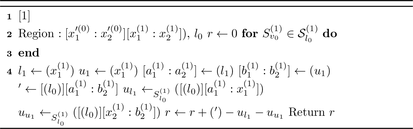
10.7 Drawing Query \(\texttt{Draw}(t)\)↩︎

Now that we have all the necessary components, we describe the algorithm for handling the \(\texttt{Draw}(t)\) query. The goal of this query is to sample an atomic region \(\rho= [x'^{(0)}_1{:}x'^{(0)}_2][x'^{(1)}_1{:}x'^{(1)}_2]\) with probability proportional to its cumulative reward: \[\frac{r(\rho)}{\sum_{\rho'} r(\rho')},\] where the summation is over all atomic regions \(\rho'\) formed over the action space \(\text{action parameter space}\).

The algorithm proceeds in two stages:

• Stage 1: Horizontal Sampling. The algorithm first samples a region of the form \(\rho_1 = [x'^{(0)}_1{:}x'^{(0)}_2][0{:}1]\), where the horizontal interval \([x'^{(0)}_1{:}x'^{(0)}_2]\) is selected with probability \[\frac{r(\rho_1)}{\sum_{\rho' \in F_t} r(\rho')}.\] This is implemented by traversing the top-level sampling tree \(\mathcal{E}^{(0)}\) from the root to a leaf \(l_0\) such that \(\texttt{Int}(l_0) = [x'^{(0)}_1{:}x'^{(0)}_2]\), querying cumulative rewards of regions of the form \([x^{(0)}_1{:}x^{(0)}_2][0{:}1]\) at each node \(v_0\) along the path \(p_{l_0}\).

• Stage 2: Vertical Sampling. Conditional on the selected region \(\rho_1\), the algorithm samples a vertical sub-region \([x'^{(1)}_1{:}x'^{(1)}_2]\) such that the full atomic region \(\rho= [x'^{(0)}_1{:}x'^{(0)}_2][x'^{(1)}_1{:}x'^{(1)}_2]\) is sampled with probability \[\frac{r(\rho)}{r(\rho_1)}.\] This step is implemented by traversing the second-level sampling tree \(\mathcal{E}^{(1)}_{l_0}\), rooted at the node corresponding to the chosen leaf \(l_0\), down to a leaf \(l_1\) such that \(\texttt{Int}(l_1) = [x'^{(1)}_1{:}x'^{(1)}_2]\), while querying cumulative rewards of regions of the form \([x'^{(0)}_1{:}x'^{(0)}_2][x^{(1)}_1{:}x^{(1)}_2]\).

  This two-stage procedure ensures that the overall sampling probability satisfies the desired marginal: \[\Pr(\rho\gets \texttt{Draw}(t)) = \frac{r(\rho)}{\sum_{\rho'} r(\rho')}.\]

10.7.1 Horizontal Sampling Stage↩︎

The algorithm begins at the root node \(v_0 = \texttt{Root}(\mathcal{E}^{(0)})\) and recursively traverses downward until reaching a leaf. At each internal node \(v_0 \in \mathcal{E}^{(0)}\), it decides whether to proceed to the left child \(\texttt{Left\_child}(v_0)\) or the right child \(\texttt{Right\_child}(v_0)\), based on the cumulative rewards of the corresponding regions.

Specifically, it moves to \(\texttt{Right\_child}(v_0)\) with probability \[\begin{align} \Pr(v_0 \gets \texttt{Right\_child}(v_0)) = \frac{r([\texttt{Int}(\texttt{Right\_child}(v_0))][0{:}1])}{r([\texttt{Int}(\texttt{Right\_child}(v_0))][0{:}1]) + r([\texttt{Int}(\texttt{Left\_child}(v_0))][0{:}1])}, \label{eq:probright} \end{align}\tag{32}\] and to \(\texttt{Left\_child}(v_0)\) with the complementary probability \(1 - \Pr(v_0 \to \texttt{Right\_child}(v_0))\).

To evaluate the required cumulative rewards, the algorithm uses the \(\texttt{CReward}^{(0)}\) query: \[\texttt{CReward}^{(0)}([\texttt{Int}(\texttt{Right\_child}(v_0))][0{:}1]) \quad \text{and} \quad \texttt{CReward}^{(0)}([\texttt{Int}(\texttt{Left\_child}(v_0))][0{:}1]).\]

This recursive process continues until a leaf node \(v_0 = l_0\) is reached, determining the atomic horizontal interval \(\texttt{Int}(l_0)\) of the sampled region.

10.7.2 Vertical Sampling Stage↩︎

To select the vertical interval, the algorithm proceeds similarly using the tree \(\mathcal{E}^{(1)}_{l_0}\), which maintains the vertical atomic intervals corresponding to the horizontal leaf \(l_0\). Starting from the root \(v_1 = \texttt{Root}(\mathcal{E}^{(1)}_{l_0})\), the algorithm recursively descends to a leaf.

At each internal node \(v_1\), the decision to move left or right is based on the cumulative reward values conditioned on the already selected horizontal interval \(\texttt{Int}(l_0)\). The probability of moving to the right child \(\texttt{Right\_child}(v_1)\) is given by: \[\begin{align} \Pr(v_1 \gets \texttt{Right\_child}(v_1)) = \frac{r([\texttt{Int}(l_0)][\texttt{Int}(\texttt{Right\_child}(v_1))])}{r([\texttt{Int}(l_0)][\texttt{Int}(\texttt{Right\_child}(v_1))]) + r([\texttt{Int}(l_0)][\texttt{Int}(\texttt{Left\_child}(v_1))])}, \label{eq:probrighty} \end{align}\tag{33}\] and the algorithm moves to \(\texttt{Left\_child}(v_1)\) with the remaining probability.

These values are computed using the \(\texttt{CReward}^{(1)}\) query: \[\texttt{CReward}^{(1)}([\texttt{Int}(l_0)][\texttt{Int}(\texttt{Right\_child}(v_1))]) \quad \text{and} \quad \texttt{CReward}^{(1)}([\texttt{Int}(l_0)][\texttt{Int}(\texttt{Left\_child}(v_1))]).\] These queries are valid since \(\texttt{Int}(l_0)\) is an atomic horizontal interval.

The process continues until a leaf node \(v_1 = l_1\) is reached in \(\mathcal{E}^{(1)}_{l_0}\), determining the atomic vertical interval \(\texttt{Int}(l_1)\). The final sampled region is then \(\rho= [\texttt{Int}(l_0)][\texttt{Int}(l_1)]\), drawn with probability proportional to its cumulative reward.

10.7.3 Hit-and-Run [32] in the Sampled Atomic Region \(\rho\)↩︎

After sampling an atomic region \(\rho= [x^{(0)}_1:x^{(0)}_2][x^{(1)}_1:x^{(1)}_2]\) via 20, we sample \(x_t \in \rho\) proportionally to \(g(x, F_t(x))\) using the Hit-and-Run algorithm. Since \(g(x, F_t(x))\) is log-concave over \(\rho\) and each atomic region is a convex subset of \(\text{action parameter space}\), the conditions of 7 are satisfied, guaranteeing efficient mixing within \(O(d^3)\) steps.

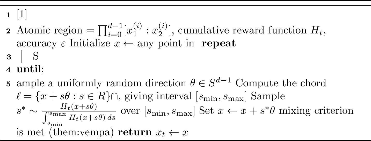
11 Correctness of the Data Structure Operations (5.2)↩︎

In this section, we prove the effectiveness of our data structure in efficiently retrieving the cumulative reward of an atomic region queried by the online learning algorithm—either \(\texttt{Weighted Majority}\) or \(\texttt{EXP3}\)—during the action selection step at round \(t\).

11.1 \(\texttt{Insert}\), \(\texttt{Update}\), and Structural Properties of \(\mathcal{T}\)↩︎

We begin by establishing the correctness of \(\texttt{Insert}\) and \(\texttt{Update}\) queries at each round. We then analyze the resulting structure to prove key properties—such as size and update complexity—that are essential for the efficiency of our data structure.

11.1.0.1 Correctness of \(\texttt{Insert}\) Query:

To insert a region \(\rho\) into our data structure, we begin by locating the atomic horizontal intervals at the leaves \(l_0\) and \(h_0\) of \(\mathcal{T}^{(0)}\) that contain the endpoints of \(\rho\)’s horizontal interval. We then split these leaves to insert the endpoints, following the standard \(\texttt{Interval Tree}\) insertion routine. This process identifies all nodes \(v_0 \in \mathcal{T}^{(0)}\) whose horizontal ranges intersect the horizontal span of \(\rho\), by traversing the root-to-leaf paths \(p_{l_0}\) and \(p_{h_0}\). As a result, the set of nodes affected by the insertion consists of two parts: (i) the nodes along the union \(p_{l_0} \cup p_{h_0}\), which are directly and regularly updated, and (ii) the nodes in the subtree rooted at the lowest common ancestor \(v_{l_0,h_0}\) that are not on these paths but are lazily affected, as their horizontal ranges lie strictly within the horizontal interval of \(\rho\). These nodes are then used to update the cumulative reward vectors post insertion to the corresponding second-level \(\texttt{Interval Tree}\)s.

Once these nodes \(v_0\) are located, we insert the vertical interval of \(\rho\) into the appropriate second-level structure—either the regular or lazy insertion \(\texttt{Interval Tree}\)—associated with each \(v_0\), as dictated by the type of insertion.

In summary, the following Observation 3 guarantees that the vertical interval of the region \(\rho\) is inserted into the appropriate regular and lazy insertion \(\texttt{Interval Tree}\)s associated with the nodes in \(\mathcal{T}^{(0)}\), thereby covering all nodes affected by the insertion of \(\rho\).

11.1.0.2 Correctness of \(\texttt{Update}\) Query:

After identifying and inserting the region \(\rho\), we proceed to update the cumulative reward information in all affected \(\texttt{Interval Tree}\)s identified during the insertion step. This ensures that each tree correctly reflects the cumulative rewards over its associated subregions. The updating routine, in either lazy or regular insertion data structures, consists of regular and lazy \(\text{reward function parameters}\) updates and lazy update messages propagation which induce slightly different properties in each though they are handled mostly similar.

We begin by characterizing the structural properties and cumulative reward updates in the regular insertion trees affected by the insertion of region \(\rho\). As noted above, all such trees \(\mathcal{T}^{(1)}_{v_0}\) correspond to nodes \(v_0 \in p_{l_0} \cup p_{h_0}\). We analyze the structure and update process by focusing on an arbitrary such node \(v_0\), as the argument applies uniformly to all affected nodes. However, a crucial distinction arises between leaf and non-leaf nodes in \(\mathcal{T}^{(0)}\). Our drawing algorithm treats these cases differently, and we correspondingly state the structural properties of \(\mathcal{T}^{(1)}_{v_0}\) through separate lemmas and observations for each type. In particular, for leaf nodes—namely \(v_0 = l_0\) or \(v_0 = h_0\)—we describe the update process through lemmas stated for \(\mathcal{T}^{(1)}_{l_0}\), which then naturally extend to \(\mathcal{T}^{(1)}_{h_0}\) and the associated regular insertion data structure of all other leaves in \(\mathcal{T}^{(0)}\).

The following corollary extends Lemma 5 to the case of lazy insertion interval trees. The result is derived similarly, based on the lazy update rule 15 . Due to the design of lazy insertion trees, the cumulative reward vector maintained at the root remains unscaled at the time of insertion. This vector is scaled appropriately during the execution of the \(\texttt{Draw}\) algorithm when it is needed for computing rewards.

We now present additional structural properties that distinguish the regular insertion trees associated with leaf versus non-leaf nodes \(v_0 \in \mathcal{T}^{(0)}\), as well as highlight key differences between the regular and lazy insertion data structures. The following Lemma 6 establishes a key structural property of the regular insertion data structures \(\mathcal{T}^{(1)}_{v_0}\) associated with the leaf nodes \(v_0 \in \mathcal{T}^{(0)}\). The proof hinges on how lazy \(\text{reward function parameters}\) updates are applied and cleared within these structures. In particular, the fact that \(v_0\) is a leaf guarantees that all updates are correctly propagated, ensuring that cumulative reward vectors stored throughout the tree are accurate and up-to-date.

We emphasize that Lemma 6 does not extend to regular insertion trees \(\mathcal{T}^{(1)}_{v_0}\) associated with non-leaf nodes \(v_0\). The key issue is that, in these cases, the lazy update messages originate from regions whose horizontal intervals may intersect only a subinterval of the node’s horizontal range \(\texttt{Int}(v_0)\), rather than fully containing it. Consequently, the cumulative lazy \(\text{reward function parameters}\) updates are no longer additive across all such regions, as the integration intervals vary and do not align uniformly with \(\texttt{Int}(v_0)\). Preserving the additivity property in this setting would require explicitly tracking the horizontal intersection of every inserted region with \(\texttt{Int}(v_0)\), significantly increasing the complexity and inefficiency of the data structure.

The intuition behind the Corollary 2 lies in the structure of the lazy insertion trees: both regular and lazy \(\text{reward function parameters}\) updates are computed by integrating over regions whose horizontal interval exactly matches \(\texttt{Int}(v_0)\). As a result, all contributions are aligned over a fixed base interval, ensuring that the cumulative reward vectors across nodes in the tree remain additive. This structural uniformity guarantees that the cumulative reward at any internal node can be decomposed into the sum of rewards over its subregions, preserving scalability for downstream computations.

Beyond these structural properties, which follow directly from the design of our \(\texttt{Insert}\) and \(\texttt{Update}\) operations, we now present two key lemmas—Lemma 3 and Lemma 4—that are fundamental to ensuring the correctness of cumulative reward retrieval. These lemmas formalize how our data structure supports exact and complete access to cumulative rewards queried by the algorithm, as detailed in the next section.

11.2 Correctness of \(\texttt{Draw}\)↩︎

In this section, we prove that the \(\texttt{Draw}\) algorithm samples an atomic region with probability proportional to its cumulative reward. As discussed earlier, \(\texttt{Draw}\) proceeds in two stages—horizontal and vertical sampling—each relying on a variant of the cumulative reward retrieval subroutine, denoted by \(\texttt{CReward}\). The correctness of \(\texttt{Draw}\) thus fundamentally depends on the correctness of these \(\texttt{CReward}\) procedures. We first analyze the two variants, \(\texttt{CReward}^{(0)}\) and \(\texttt{CReward}^{(1)}\), in order. Prior to that, we establish two key structural lemmas—Lemmas 3 and 4—which underpin the correctness and simplify the subsequent analysis.

11.2.0.1 Uniqueness and Completeness of the \(\texttt{Interval Tree}\)s

We now analyze two fundamental structural properties—uniqueness and completeness—that are critical to the correctness of our cumulative reward retrieval procedures. When handling a \(\texttt{CReward}\) query, either \(\texttt{CReward}^{(0)}\) or \(\texttt{CReward}^{(1)}\), for a rectangular region \(\rho: [x^{(0)}_1:x^{(0)}_2][x^{(1)}_1:x^{(1)}_2]\), the algorithm identifies all data structures that contain cumulative reward information relevant to regions intersecting \(\rho\). It then extracts the corresponding contributions—either directly or via scaling—and aggregates them to compute the cumulative reward over \(\rho\). To ensure correctness, two conditions must be met: First, uniqueness—each intersecting region must contribute through exactly one of the collected data structures to avoid double-counting. Second, completeness—all regions that intersect \(\rho\) must be represented within the union of the collected data structures; omitting any such region would lead to inaccurate estimates. The following lemmas formalize and prove these two properties.

To retrieve the cumulative reward of a region \(\rho: [x^{(0)}_1:x^{(0)}_2][x^{(1)}_1:x^{(1)}_2]\), our algorithm first identifies the node \(v_0 \in \mathcal{T}^{(0)}\) whose horizontal range minimally contains \([x^{(0)}_1:x^{(0)}_2]\). It then constructs the set \(\mathcal{S}^{(1)}_{v_0}\) of second-level interval trees relevant for querying the vertical interval. This set includes the regular insertion tree \(\mathcal{T}^{(1)}_{v_0}\), as well as lazy insertion trees associated with the ancestors \(v_0'\) of \(v_0\) along the path to the root: if \(v_0\) lies in the left (resp., right) subtree of \(v_0'\), we include \(\mathcal{L}^{(1)}_{v_0'}\) (resp., \(\mathcal{R}^{(1)}_{v_0'}\)) in \(\mathcal{S}^{(1)}_{v_0}\). We refer to each element in this set by \(S_{v'_0}\), denoting the second-level data structure associated with the ancestor \(v'_0\). The complete construction of \(\mathcal{S}^{(1)}_{v_0}\) is detailed in Section 10.6 and Algorithm 16.

Now, the following Lemmas 3 and 4 guarantee the uniqueness and completeness of \(\mathcal{S}_{v_0}\) for any node \(v_0 \in \mathcal{T}^{(0)}\).

Lemmas 3 and 4 guarantee a disjoint and complete organization of the second-level data structures that either directly or lazily affect a node \(v \in \mathcal{T}^{(0)}\), denoted by \(\mathcal{S}_v\) in Algorithm 16. This structural property enables efficient and modular handling of cumulative reward queries. A key observation is that each lazy data structure in \(\mathcal{S}_v\) uniformly influences its corresponding subtree, and thus can be queried independently. Combined with the scaling technique introduced in Section 7.1, which preserves correctness while mapping contributions from various structures to the target range of \(v\), this design avoids redundant insertions at every round.

With the structural properties established in Lemmas 3 and 4, we are now ready to formally prove the correctness of Algorithm 17 and 18, which implements the cumulative reward retrieval procedure \(\texttt{CReward}\). These lemmas ensure that all relevant contributions to the cumulative reward of a given query region are uniquely and completely represented within the data structures comprising \(\mathcal{S}^{(1)}_{v_0}\), thereby enabling accurate and efficient computation via \(\texttt{CReward}\).

11.2.0.2 Correctness of \(\texttt{CReward}\) Query:

As previously discussed, the cumulative reward retrieval procedure \(\texttt{CReward}\) is decomposed into two specialized subroutines, \(\texttt{CReward}^{(0)}(\cdot)\) and \(\texttt{CReward}^{(1)}(\cdot)\), for handling queries in the two-dimensional action space. These are detailed in Section 10.6. We now formally establish the correctness of each subroutine through the following lemmas.

11.2.0.3 Correctness of \(\texttt{Draw}\) Query

In this section we prove that our drawing Algorithm 19 and 20 finds an atomic region with the correct probability.

12 Generalization to \(d\)-dimensions (5)↩︎

We now extend this construction recursively to a \(d\)-layered data structure, denoted by \(\mathcal{T}\). The outermost layer is \(\mathcal{T}^{(0)}\), whose nodes \(v_0 \in \mathcal{T}^{(0)}\) each maintain three second-level data structures: a regular structure \(\mathcal{T}^{(1)}_{v_0}\), and two lazy structures \(\mathcal{L}^{(1)}_{v_0}\) and \(\mathcal{R}^{(1)}_{v_0}\). This organization is applied recursively to all levels: every node \(v_1\) in the second level structures (i.e., in \(\mathcal{T}^{(2)}_{v_0,v_1}\), \(\mathcal{L}^{(1)}_{v_0,v_1}\), or \(\mathcal{R}^{(1)}_{v_0,v_1}\)) maintains its own set of third-level structures, namely \(\mathcal{T}^{(2)}_{v_0,v_1}\), \(\mathcal{L}^{(2)}_{v_0,v_1}\), and \(\mathcal{R}^{(2)}_{v_0,v_1}\), following the same pattern and details as in the warm-up case.

This recursive structure continues until the \((d-1)\)-th level. In general, for any node \(v_i\) at the \(i\)-th level, we maintain: \[\mathcal{T}^{(i+1)}_{v_0, v_1, \dots, v_i}, \quad \mathcal{L}^{(i+1)}_{v_0, v_1, \dots, v_i}, \quad \mathcal{R}^{(i+1)}_{v_0, v_1, \dots, v_i}.\] At the \(d\)-th level, the leaf nodes store all required information regarding the region’s cumulative rewards stored as vectors \(\vec{r}\). Specifically, for each node \(v_{d-1}\) in a \(d\)-th level tree, we store \[\vec{r}_{v_0, \dots, v_{d-1}},\] which encode the cumulative rewards for their corresponding subregions and are used for scaling and lazy propagation in higher-level queries.

Next, we describe how the operations \(\texttt{Insert}\), \(\texttt{Update}\), \(\texttt{CReward}\), and \(\texttt{Draw}\) are performed in this recursive setting for a given region \(\rho\) of the form: \[\rho= [x^{(0)}_1:x^{(0)}_2][x^{(1)}_1:x^{(1)}_2]\cdots[x_1^{(d-1)}:x_2^{(d-1)}].\]

12.1 \(\texttt{Insert}(\rho)\)↩︎

We begin by locating the interval \([x^{(0)}_1:x^{(0)}_2]\) of the region \(\rho\) along the first coordinate in \(\mathcal{T}^{(0)}\). We identify the corresponding leaf nodes \(l_0\) and \(u_0\), and compute their lowest common ancestor, denoted by \(v_{l_0,u_0}\). We then follow the same insertion procedure as described in Algorithm 7. Specifically, we traverse the nodes \(v_0\) along the paths \(p_{l_0}\), \(p_{u_0}\), and \(p_{v_{l_0,u_0}}\) in a bottom-up manner. For each such node \(v_0 \in \mathcal{T}^{(0)}\), we insert the remaining coordinate intervals \[[x^{(1)}_1:x^{(1)}_2], \dots, [x^{(d-1)}_1:x^{(d-1)}_2]\] into one of the associated second-level data structures: \(\mathcal{T}^{(1)}_{v_0}\), \(\mathcal{L}^{(1)}_{v_0}\), or \(\mathcal{R}^{(1)}_{v_0}\), depending on whether \(v_{l_0,u_0}\) lies in the left or right subtree of \(v_0\).

We apply this process recursively at deeper levels. For each node \(v_0\), we locate the interval \([x^{(1)}_1:x^{(1)}_2]\) within its associated second-level tree, identify the corresponding leaves \(l_1\) and \(u_1\), and determine their lowest common ancestor \(v_{l_1,u_1}\). We then traverse the paths \(p_{l_1}\), \(p_{u_1}\), and \(p_{v_{l_1,u_1}}\), and insert the remaining intervals \([x^{(2)}_1:x^{(2)}_2], \dots, [x^{(d-1)}_1:x^{(d-1)}_2]\) into the appropriate third-level data structure: \(\mathcal{T}^{(2)}_{v_0,v_1}\), \(\mathcal{L}^{(2)}_{v_0,v_1}\), or \(\mathcal{R}^{(2)}_{v_0,v_1}\).

This recursive procedure continues until we reach the \((d{-}1)\)-th level. There, the final interval \([x^{(d-1)}_1:x^{(d-1)}_2]\) is inserted into one of the data structures: \[\mathcal{T}^{(d-1)}_{v_0, v_1, \dots, v_{d-2}},\quad \mathcal{L}^{(d-1)}_{v_0, v_1, \dots, v_{d-2}},\quad \text{or} \quad \mathcal{R}^{(d-1)}_{v_0, v_1, \dots, v_{d-2}}.\]

12.2 \(\texttt{Update}(\rho)\)↩︎

To handle this query, we once again locate the affected nodes in each layer—specifically, those that were identified and inserted into their respective lazy or regular data structures during the \(\texttt{Insert}\) query. Suppose we reach the \(d\)-th level tree after traversing the sequence of nodes \(v_0, v_1, \dots, v_{d-2}\), arriving at \(\mathcal{T}^{(d-1)}_{v_0,v_1,\dots,v_{d-2}}\). In this tree, we locate the leaves corresponding to the endpoints of the interval \([x_1^{(d-1)}:x_2^{(d-1)}]\), denoted by \(l_{d-1}\) and \(u_{d-1}\), respectively. Their first common ancestor is referred to as \(v_{l_{d-1},u_{d-1}}\). We then traverse the nodes \(v_{d-1}\) along the paths \(p_{l_{d-1}}\), \(p_{u_{d-1}}\), and \(p_{v_{l_{d-1},u_{d-1}}}\), and at each such node, compute the following vector \(\vec{A}_{\rho'},\) for \(\rho' = [\texttt{Int}(v_0)],[\texttt{Int}(v_1)],\dots,[\texttt{Int}(v_{d-1})]\), where each vector \(\vec{A}^{(i)}_{\rho'}\) is computed according to equation 4 , using the coefficient vector \(f_t(\rho)\) and then aggregate it with the \(\vec{r}_{v_0,v_1,\cdots,v_{d-1}}\) to update it. As in the warm-up case, we then update the reward vector \(\vec{r}_{v_0,v_1,\dots,v_{d-1}}\) at each visited node with the value \(f_t(\rho)\). The update process, including the lazy update messages, follows exactly the same rule as in the warm-up case.

12.3 \(\texttt{CReward}(\rho)\)↩︎

Handling this query efficiently is central to extending the methods developed in the warm-up case to the general \(d\)-dimensional axis-parallel setting. As introduced earlier, our drawing algorithm decomposes a cumulative reward query into a sequence of subqueries of the form: \[\begin{align} &\texttt{CReward}^{(0)}\left(\rho: [x^{(0)}_1:x^{(0)}_2][0:1] \cdots [0:1]\right),\\ &\texttt{CReward}^{(1)}\left(\rho: [x'^{(0)}_1:x'^{(0)}_2][x^{(1)}_1:x^{(1)}_2][0:1] \cdots [0:1]\right),\\ &\quad \vdots\\ &\texttt{CReward}^{(d-1)}\left(\rho: [x'^{(0)}_1:x'^{(0)}_2][x'^{(1)}_1:x'^{(1)}_2] \cdots [x'^{(d-2)}_1:x'^{(d-2)}_2][x^{(d-1)}_1:x^{(d-1)}_2]\right), \end{align}\] where each \([x'^{(i)}_1:x'^{(i)}_2]\) is an atomic interval along the \(i\)-th coordinate, fixed during the \(i\)-th stage of the drawing process. While the mechanics of each subquery follow the warm-up case, the challenge in higher dimensions lies in identifying the correct set of data structures and ensuring the cumulative reward vectors they store can be accurately scaled.

At each stage \(i+1\), a key step is to gather all relevant \((i+1)\)-th level data structures that affect the current subspace: \[[x'^{(0)}_1:x'^{(0)}_2],\;[x'^{(1)}_1:x'^{(1)}_2],\;\dots,\;[x'^{(i{-}1)}_1:x'^{(i{-}1)}_2],\;[0:1],\;\dots,\;[0:1].\] These structures are assembled into the set \(\mathcal{D}^{(i)}_{l_0, l_1, \dots, l_{i{-}1}}\), where each \(l_j\) is a leaf node in the auxiliary tree \(\mathcal{E}^{(j)}\) with \(\texttt{Int}(l_j) = [x'^{(j)}_1:x'^{(j)}_2]\). This naming reflects the assumption that each \(\texttt{Int}(l_j)\) is an atomic interval—that is, one stored entirely at a leaf node.

The construction of \(\mathcal{D}^{(i)}_{l_0, l_1, \dots, l_{i{-}1}}\) proceeds recursively. We begin by locating the leaf \(l'_0 \in \mathcal{T}^{(0)}\) such that \(\texttt{Int}(l'_0) \subseteq \texttt{Int}(l_0)\), and then traverse its ancestor path \(p_{l'_0}\) to collect all relevant lazy insertion structures, as described in the warm-up case.

For each structure collected at the first level, we repeat the process at the second level: we locate a leaf \(l'_1\) such that \(\texttt{Int}(l'_1) \subseteq \texttt{Int}(l_1)\), traverse its ancestor path \(p_{l'_1}\), and gather all associated lazy insertion structures. This continues recursively: at each newly collected structure from level \(j-1\), we locate the leaf containing \(\texttt{Int}(l_j)\), traverse upward, and collect relevant structures at level \(j+1\), for \(j = 2, \dots, i-1\).

The recursion terminates when all \(i\)-th level structures are collected whose root’s associated region fully contains the subspace: \[[x'^{(0)}_1:x'^{(0)}_2],\;[x'^{(1)}_1:x'^{(1)}_2],\;\dots,\;[x'^{(i{-}1)}_1:x'^{(i{-}1)}_2],\;[0:1],\;\dots,\;[0:1].\] Each such structure is denoted by \(D^{(i)}_{v'_0, v'_1, \dots, v'_{i{-}1}}\), where \(v'_j\) is a node on the path \(p_{l'_j}\). The structure \(D^{(i)}_{v'_0, \dots, v'_{i{-}1}}\) is then added to the set \(\mathcal{D}^{(i)}_{l_0, l_1, \dots, l_{i{-}1}}\). Due to the recursive construction, we can show that the size of this set satisfies: \[\abs{\mathcal{D}^{(i)}_{l_0, l_1, \dots, l_{i{-}1}}} \in O(\log^i t).\]

Once \(\mathcal{D}^{(i)}_{l_0, \dots, l_{i{-}1}}\) is formed, the algorithm evaluates: \[\texttt{CReward}^{(i)}\left(\rho: [x'^{(0)}_1:x'^{(0)}_2] \cdots [x'^{(i{-}1)}_1:x'^{(i{-}1)}_2][x^{(i)}_1:x^{(i)}_2][0:1] \cdots [0:1]\right)\] for each data structure \(D^{(i)}_{v'_0, v'_1, \dots, v'_{i{-}1}}\) in the set, and aggregates the results to identify the next atomic interval along the \((i+1)\)-th coordinate.

To ensure correctness, we must verify that the vectors stored in the \(d{-}1\)-th level of each \(D^{(i)}_{v'_0, \dots, v'_{i{-}1}}\) can be properly scaled to the subregion defined by the first \(i\) atomic intervals: \[[x'^{(0)}_1:x'^{(0)}_2],\;[x'^{(1)}_1:x'^{(1)}_2],\;\dots,\;[x'^{(i{-}1)}_1:x'^{(i{-}1)}_2][0:1]\cdots[0:1].\] This guarantee follows inductively from the way the data structures are collected. For each coordinate index \(j < i\), the interval \(\texttt{Int}(l_j)\) lies entirely within a single leaf \(l'_j\). As we construct \(\mathcal{D}^{(i)}_{l_0, \dots, l_{i{-}1}}\), we only include lazy structures along ancestor paths from these leaves. Since each lazy structure supports proper scaling over any subregion it contains, the cumulative reward vectors can be scaled correctly at every step. By applying this argument inductively over all \(j < i\), we conclude that all vectors stored in structures from \(\mathcal{D}^{(i)}_{l_0, \dots, l_{i{-}1}}\) can be scaled to the region above. This inductive scaling property allows the drawing algorithm to proceed sequentially across coordinates, correctly and efficiently identifying one atomic interval at a time.

12.4 \(\texttt{Draw}(t)\)↩︎

The drawing procedure in the \(d\)-dimensional setting extends naturally from the warm-up case. It proceeds in \(d\) sequential stages, where at each stage \(i \in \{0, 1, \dots, d{-}1\}\), the algorithm identifies an atomic interval along the \(i\)-th coordinate using the corresponding auxiliary tree \(\mathcal{E}^{(i)}\). Each tree is traversed via a probabilistic descent based on cumulative reward values, thereby selecting the appropriate atomic interval.

The process begins by locating the atomic horizontal interval \([x'^{(0)}_1:x'^{(0)}_2]\) using the query: \[\texttt{CReward}^{(0)}\left([x^{(0)}_1:x^{(0)}_2][0:1]\cdots[0:1]\right).\] Conditioned on this horizontal slice, the algorithm continues to the second stage, identifying the atomic interval \([x'^{(1)}_1:x'^{(1)}_2]\) via: \[\texttt{CReward}^{(1)}\left([x'^{(0)}_1:x'^{(0)}_2][x^{(1)}_1:x^{(1)}_2][0:1]\cdots[0:1]\right).\] More generally, for stage \(i\), the query has the form: \[\texttt{CReward}^{(i)}\left([x'^{(0)}_1:x'^{(0)}_2] \cdots [x'^{(i{-}1)}_1:x'^{(i{-}1)}_2][x^{(i)}_1:x^{(i)}_2][0:1] \cdots [0:1]\right),\] which returns the cumulative reward necessary to sample the atomic interval \([x'^{(i)}_1:x'^{(i)}_2]\).

This routine continues recursively until the final atomic interval \([x'^{(d{-}1)}_1:x'^{(d{-}1)}_2]\) is selected, resulting in the sampled region \(\rho= [x'^{(0)}_1:x'^{(0)}_2]\cdots[x'^{(d{-}1)}_1:x'^{(d{-}1)}_2]\).

13 Time Complexity (5.2)↩︎

We begin by recalling the time complexity of standard multi-dimensional range trees (\(\texttt{Range Tree}\)) that report the set of points within a queried axis-aligned rectangular region. Our multi-dimensional data structure follows a similar hierarchical construction but maintains intervals instead of points. Provided that \(\mathcal{T}\) remains balanced by 2, we can adopt the classical bounds for \(\texttt{Insert}\) and \(\texttt{Update}\). Due to lazy insertions and the fact that not all intervals are explicitly stored in associated next-level trees, the time complexity for \(\texttt{CReward}\) and \(\texttt{Draw}\) deviates slightly; we address these distinctions below.

13.1 Time complexity of \(\texttt{Insert}(.)\)↩︎

13.2 Time complexity of \(\texttt{Update}(.)\)↩︎

13.3 Time complexity of \(\texttt{CReward}(\rho)\)↩︎

As described earlier, the cumulative reward query \(\texttt{CReward}(\rho)\) is decomposed into a sequence of subqueries \(\texttt{CReward}^{(i)}(\rho)\), each operating on progressively more refined regions. In each \(\texttt{CReward}^{(i)}\) subquery, the first \(i\) intervals along the first \(i\) coordinates are atomic, fixed by earlier sampling stages, while the remaining \(d-i\) intervals span the full range \([0:1]\). The time complexity depends on the number of data structures in \(\mathcal{S}^{(i)}_{l_0,\dots,l_{i-1}}\), each of which must be queried and aggregated to compute the final cumulative reward.

13.4 Time Complexity of Hit-and-Run [32]↩︎

By 7, this step takes \(O\left(d^3 \log\left( \frac{Y}{\varepsilon} \right)\right).\)

13.4.1 Time Complexity of \(\texttt{Draw}(t)\)↩︎

13.5 Memory Complexity↩︎

14 Efficient Adversarial Online Learning: Overview (6)↩︎

We consider the adversarial online learning setting where at each round \(t\), a \(\sigma\)-smoothed adversary selects hyperplanes \(\Psi_t\) and assigns a piecewise-structured reward function \(h_t\) over the induced partition \(\mathcal{P}_t\) of \([0,1]^d\), with \(g\) fixed and known. The learner selects action \(x_t\) by sampling proportionally to \(\zeta(H_t(x)) = \exp(\eta g(x, F_t(x)))\), where \(F_t(x) = \sum_{t' \leq t} f_{t'}(x)\) is the cumulative parameter function maintained by \(\mathcal{T}\), instantiating our proportional sampling framework of 5 with exponential weighting. Beyond efficient sampling, the central objective is regret minimization: given a time horizon \(T\) and actions \(x_1, \dots, x_T \in [0,1)^d\), the regret of policy \(\pi\) is \[\begin{align} \operatorname{Regret}(\pi, T) \doteq \max_{x \in [0,1]^d} g(x, F_T(x)) - \mathop{\mathrm{\mathbb{E}}}\!\left[\sum_{t=1}^T g(x_t, f_t(x_t))\right], \end{align}\]

We consider two feedback models: under full-information feedback the learner observes the full specification of \(h_t\) over all regions at each round, while under bandit feedback only \(h_t(\rho_{i,t})\) for the region containing \(x_t\) is revealed, implicitly disclosing both the structure and real-valued reward of that region. In the following subsections, we present the detailed data structure, query handling, computational challenges of proportional sampling under each feedback model, and the corresponding regret and time complexity analyses, together constituting the proofs of 3 and 4.

15 Full-Information Feedback: Data Structure, Regret, and Time Complexity (6)↩︎

Under full-information feedback, the mapping function \(g\) is fixed and known throughout, and at each round the learner receives the full specification of \(f_t\) over all regions of \(\mathcal{P}_t\). The learner then selects action \(x_t\) by sampling proportionally to \(\zeta(H_t(x)) = \exp(\eta g(x, F_t(x)))\) over \([0,1]^d\), where \(F_t(x) = \sum_{t' \leq t} f_{t'}(x)\) is the cumulative parameter function maintained by \(\mathcal{T}\). The online learning algorithm employed in this setup is \(\texttt{Weighted Majority}\), a no-regret algorithm that selects \(x_t\) at each round with probability proportional to the exponential of its cumulative reward, whose pseudocode is presented in 22.

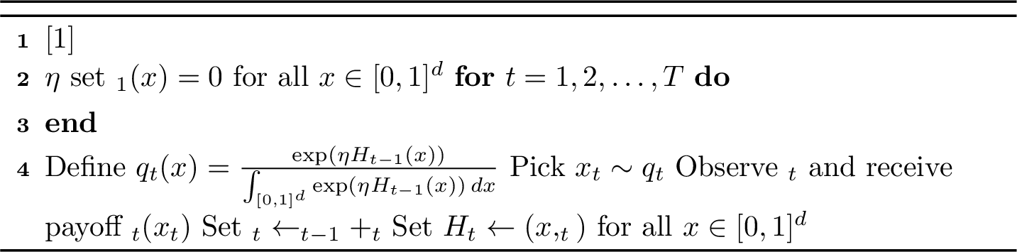
Handling proportional sampling for \(\texttt{Weighted Majority}\) under the adversarial model of 3 introduces two main challenges: the non-linearity of \(\exp\) breaks the additive structure of cumulative reward vectors that made lazy insertion and deferred scaling efficient, and no closed-form aggregate reward formula exists beyond degree one, making exact integration and regret bounding intractable for higher-degree rewards. These challenges require us to restrict the adversary from the full generality of 3, as detailed below.

15.1 Challenges of Proportional Sampling under with the Adversarial Smoothness of Model 3↩︎

15.1.0.1 Non-additivity under \(\exp\) compared to polynomials.

Similar to the proportional sampling case with \(\zeta(x) = x\), efficient sampling under \(\zeta(x) = \exp(\eta x)\) requires lazy insertion data structures and scaling techniques to avoid an excessive number of insertions at each round. However, lazy insertions interact poorly with the exponential form of \(\zeta\), introducing a fundamental obstacle that prevents direct application of the same approach. When \(\zeta(x) = x\), the feedback parameter \(f_t\) serves as the coefficient of monomials in \(g\) and remains additive across rounds, allowing cumulative rewards \(r\) to be efficiently aggregated over disjoint regions and making scaling operations both sound and efficient. Under \(\zeta(x) = \exp(\eta x)\), however, \(\text{reward function parameters}\) appears in the exponent, so the cumulative reward over a union of regions is no longer the sum of individual rewards. This breaks the additive property essential to our scaling technique: any attempt to merge disjoint structures while deferring insertions requires identifying all atomic regions formed by their union, a task computationally equivalent to performing all insertions upfront.

As illustrated in Example 3, this obstacle is inherent to any lazy insertion scheme under \(\zeta(x) = \exp(\eta x)\): combining information from disjoint structures during sampling necessitates detecting the resulting atomic regions and re-integrating over them, effectively undoing the savings achieved by deferring insertions. To circumvent this, we restrict the adversary to selecting hyperplanes along all but one coordinate from fixed sets of at most \(M\) hyperplanes, ensuring that the overlay structure between lazy and regular trees is known in advance and remains static throughout.

15.1.0.2 Non-existence of closed-form aggregate reward \(r(\rho)\) for \(g\) of degree higher than one.

For polynomial \(g\) of degree \(n \geq 2\), no closed-form expression for \(r(\rho) = \int_{\rho} \exp(\eta g(x, F_t(x)))\,dx\) exists in general. For instance, when \(g(x, F_t(x)) = F_t^{(0)} (x^{(0)})^2 + F_t^{(1)} x^{(1)}\), the integral \(\int \exp(\eta F_t^{(0)} (x^{(0)})^2)\,dx\) is related to the Gaussian integral and admits no elementary antiderivative. Consequently, \(r(\rho)\) cannot be computed analytically or stored exactly in \(\mathcal{T}\) for \(n \geq 2\), making both efficient data structure maintenance and regret analysis infeasible beyond degree one.

15.1.0.3 Computational inefficiency of scaling under piecewise-linear rewards \(h_t\).

Unlike high-degree polynomials, a closed-form expression for the aggregate reward of a region does exist for piecewise-linear \(g\): for an axis-parallel rectangular region \[\rho= [x^{(0)}_1:x^{(0)}_2][x^{(1)}_1:x^{(1)}_2] \cdots [x^{(d-1)}_1:x^{(d-1)}_2],\] with \(H_t(x)\) linear over \(\rho\) and cumulative feedback vector \(F_t = \langle F_t^{(0)}, F_t^{(1)}, \ldots, F_t^{(d-1)} \rangle\), the exponentially weighted cumulative reward is given by \[\begin{align} r(\rho) = \int_{\rho} \exp(\eta h_t(x)) \, dx = \prod_{i=0}^{d-1} \begin{cases} \displaystyle\frac{\exp(\eta F_t^{(i)} x^{(i)}_2) - \exp(\eta F_t^{(i)} x^{(i)}_1)}{\eta F_t^{(i)}}, & \text{if } F_t^{(i)} \ne 0, \\[1.2ex] x^{(i)}_2 - x^{(i)}_1, & \text{if } F_t^{(i)} = 0. \end{cases} \label{eq:expint} \end{align}\tag{37}\] However, the presence of \(F_t^{(i)}\) in the denominator couples all \(\text{reward function parameters}\) components across coordinates: to scale a stored cumulative reward from a parent region down to a subregion, each internal node would require access to \(F_t^{(i)}\) for every atomic subregion in its subtree, since \(F_t^{(i)}\) varies across atomic regions and the exponential terms cannot be factored or cancelled without knowing it explicitly. As the number of atomic subregions in a subtree grows as \(O(t)\), this incurs an \(O(t)\) cost per node per round, making efficient maintenance infeasible.

15.2 Full-Information Setup and Adversarial Model↩︎

In response to the computational challenges detailed in 15.1, we restrict the adversary and reward structure for the full-information setting as follows. Due to the non-additivity of \(\exp(\eta H_t(x))\) across lazy and regular structures, we restrict to piecewise-constant rewards, and due to the \(O(t)\) cost of resolving disjoint endpoint sets across structures in \(\mathcal{S}^{(1)}_{v_0}\), we restrict the adversary to smooth hyperplane selection along one designated direction only.

15.2.0.1 Full-Information Setup.

Concretely, at each round \(t\), \(k\) hyperplanes \(\Psi_t = \{\psi_{1,t}, \dots, \psi_{k,t}\}\) are chosen with directions from \(\Gamma\) as in 3, with the following modification: for each \(\psi_{j,t} \in \Psi_t\), if \(\psi_{j,t}\) is parallel to \(\gamma_1 \in \Gamma\), it is drawn smoothly from \(\mathcal{D}^{(1)}_t\) over \([0,1]\), with the total number of such hyperplanes growing to \(TK\) over time; otherwise it is chosen from a fixed set \(\mathcal{M}^{(i)} = \{\psi^{(i)}_1, \dots, \psi^{(i)}_M\}\) of at most \(M\) hyperplanes defined a priori for each direction \(\gamma_i \in \Gamma\setminus \{\gamma_1\}\). Without loss of generality, \(\gamma_1\) corresponds to the first coordinate of \(\text{action parameter space}\); otherwise the coordinate axes are permuted accordingly. The hyperplanes \(\Psi_t\) then partition \([0,1]^d\) into regions \(\mathcal{P}_t\), over which the adversary assigns a piecewise-constant reward \(h_t\).

Under this restriction, only the number of hyperplanes along \(\gamma_1\) grows linearly with time, while the number of intervals along all remaining directions stays bounded by \(M\) throughout. This allows us to retain the same structure of lazy and regular insertions with significantly lower overhead: since the boundaries along the remaining \(d-1\) coordinates are known a priori, handling updates and scaling operations does not incur a worst-case cost of \(O(t^d)\) per round but instead reduces to \(O(M^d)\), where \(M\) is the size of the fixed hyperplane sets. In particular, the overlay structure between lazy and regular trees is fixed in advance, eliminating the costly atomic region detection that arises in the general case.

15.3 Data Structure and Query Handling for \(\texttt{Weighted Majority}\) under Full-Information Feedback↩︎

We now describe how queries are handled to maintain efficiency when sampling \(x_t\) under piecewise constant reward functions. We present the construction in the two-dimensional case; the \(d\)-dimensional generalization follows the same layered approach as 12 with adjusted time complexity and regret bounds.

The first-level tree \(\mathcal{T}^{(0)}\) organizes the unique dynamic coordinate, along which the adversary introduces new hyperplanes over time. Each node \(v_0 \in \mathcal{T}^{(0)}\) maintains three second-level interval trees over the second coordinate: a regular insertion tree \(\mathcal{T}^{(1)}_{v_0}\) and two lazy insertion trees \(\mathcal{L}^{(1)}_{v_0}\) and \(\mathcal{R}^{(1)}_{v_0}\), mirroring the structure of 5. This setting, however, differs from the general construction in three key respects:

• Fixed-grid trees at all deeper levels. Since the adversary’s hyperplanes along all remaining coordinates are drawn from fixed sets \(\mathcal{M}^{(1)}, \dots, \mathcal{M}^{(d-1)}\) of at most \(M\) hyperplanes each, all second-level trees are initialized once over this fixed grid and remain static throughout, each containing \(O(M)\) nodes. In the \(d\)-dimensional case, these become \((d{-}1)\)-dimensional regular interval trees, each organized over the fixed grid \(\mathcal{M}^{(1)} \times \cdots \times \mathcal{M}^{(d-1)}\) and containing \(M^{d-1}\) nodes per first-level node.

• Lazy structures at the first level only. Since no new hyperplanes are introduced along any coordinate beyond the first, no deferred insertions arise at deeper levels. Lazy structures \(\mathcal{L}^{(1)}_{v_0}\) and \(\mathcal{R}^{(1)}_{v_0}\) are therefore maintained exclusively at nodes \(v_0 \in \mathcal{T}^{(0)}\), with no lazy components at any level beyond \(\mathcal{T}^{(0)}\). In the \(d\)-dimensional case, this remains unchanged: lazy structures are attached solely to nodes of \(\mathcal{T}^{(0)}\), and all trees at levels \(i \geq 1\) are purely regular.

• Scalar Cumulative Rewards rather than Vectorized. Since \(H_t\) is piecewise-constant over each atomic region \(\rho= \prod_{i=0}^{d-1}[x_1^{(i)}{:}x_2^{(i)}]\) with constant value \(c_{\rho} \in \mathbb{R}_{\geq 0}\), the exponentially weighted cumulative reward of \(\rho\) takes the closed form \[\begin{align} r(\rho) = \int_{\rho} \exp\!\left(\eta\, H_t(x)\right) dx = \exp(\eta\, c_{\rho}) \cdot \prod_{i=0}^{d-1}(x_2^{(i)} - x_1^{(i)}), \label{eq:expintconst} \end{align}\tag{38}\] a single exponential factor multiplied by a product of interval lengths. Since scaling is required only along the first coordinate, this separable form means that all nodes in every second-level tree need only maintain a scalar value rather than a reward vector, while fully preserving the scalability needed for efficient updates.

We now specify the scalar quantities maintained at each node of the regular and lazy second-level trees.

15.3.0.1 Exponentially Weighted Cumulative Reward for Regular Insertion Data Structures.

Each node \(v_1\) in the regular insertion tree \(\mathcal{T}^{(1)}_{v_0}\) maintains a scalar \(r_{v_0,v_1}\), aggregating the exponentially weighted cumulative reward over all regions \(\rho= [c^{(0)}_1:c^{(0)}_2][c^{(1)}_1:c^{(1)}_2]\) whose horizontal projection contains at least one endpoint in \(\texttt{Int}(v_0)\) and whose vertical projection is contained in \(\texttt{Int}(v_1)\), that is, \[\begin{align} r_{v_0,v_1} = \sum_{\rho} r\!\left([\texttt{Int}(v_0) \cap [c^{(0)}_1:c^{(0)}_2]]\, [\texttt{Int}(v_1)\cap[c^{(1)}_1:c^{(1)}_2]]\right), \label{eq:cr-regular} \end{align}\tag{39}\] where \(r(\cdot)\) is as defined in 38 .

15.3.0.2 Cumulative Feedback Parameters for Lazy Insertion Data Structures.

Each node \(w_1\) in the lazy insertion trees \(\mathcal{L}^{(1)}_{v_0}\) or \(\mathcal{R}^{(1)}_{v_0}\) maintains a scalar \(r_{v_0,w_1}\), aggregating the exponentially weighted cumulative reward over all regions \(\rho= [c^{(0)}_1:c^{(0)}_2][c^{(1)}_1:c^{(1)}_2]\) whose horizontal projection fully contains the range of the corresponding child of \(v_0\) (i.e., \(\texttt{Int}(\texttt{Left\_child}(v_0))\) for \(\mathcal{L}^{(1)}_{v_0}\) and \(\texttt{Int}(\texttt{Right\_child}(v_0))\) for \(\mathcal{R}^{(1)}_{v_0}\)) and whose vertical projection is contained in \(\texttt{Int}(w_1)\), that is, \[\begin{align} r_{v_0,w_1} = \sum_{\rho} r\!\left([\texttt{Int}(v_0)]\, [[c^{(1)}_1:c^{(1)}_2] \cap \texttt{Int}(w_1)]\right), \label{eq:cr-lazy} \end{align}\tag{40}\] where \(r(\cdot)\) is as defined in 38 , and the sum ranges over all lazily inserted regions as defined in 5.1. Since all lazily inserted regions contribute uniformly over \(\texttt{Int}(v_0)\), this value scales consistently to any subinterval of \([\texttt{Int}(v_0)]\), including \(\texttt{Int}(\texttt{Left\_child}(v_0))\) and \(\texttt{Int}(\texttt{Right\_child}(v_0))\), without requiring recomputation.

15.3.0.3 Handling \(\texttt{Insert}\), \(\texttt{Update}\), and \(\texttt{Draw}\).

The \(\texttt{Insert}\) and \(\texttt{Update}\) routines follow the same locate-and-traverse approach as described in 5.1 for the main structure. Specifically, at the first level, \(\texttt{Insert}(\rho)\) locates the boundary leaves in \(\mathcal{T}^{(0)}\) and traverses upward to identify the relevant regular and lazy second-level structures, exactly as before. Within each second-level tree, updates to the scalar values \(r_{v_0,v_1}\) and \(r_{v_0,w_1}\) follow the standard lazy propagation technique common in the interval tree literature [13].

15.3.0.4 Different Proportional Sampling \(\texttt{Draw}\).

The \(\texttt{Draw}(t)\) procedure follows the same two-step sampling scheme as in 5.2: first a horizontal atomic interval is sampled from \(\mathcal{T}^{(0)}\), then a vertical atomic interval is sampled conditioned on the horizontal selection. This procedure, however, differs from the general case in three key respects:

• Modified \(\texttt{CReward}\) subroutine. In the general structure, the additivity of \(\zeta(x) = x\) allows \(\texttt{CReward}\) to aggregate cumulative reward across lazy and regular structures via clean vector arithmetic. Under \(\zeta(x) = \exp(\eta x)\), this additivity is lost, necessitating a fundamentally different approach. We exploit the fact that all second-level trees are organized over a fixed set of \(M\) endpoints along each remaining coordinate: rather than aggregating across structures symbolically, \(\texttt{CReward}\) iterates explicitly over all \(O(M)\) leaves of the second-level trees, applies the exponential scaling to each leaf individually, and sums the resulting scalar values bottom-up to recover the correct aggregated cumulative reward. This leaf-wise scaling and summation procedure is what replaces the vector-based aggregation of the general case and is detailed in the scaling procedure below.

• Exponential scaling. Rather than scaling via linear vector arithmetic as in the general structure, lazy contributions stored in ancestor nodes along \(p_{v_0}\) are propagated multiplicatively as \(\exp(\eta \cdot r_{v_0,w_1})\), correctly incorporating deferred additive feedback parameter shifts into the exponent of the cumulative reward. This scaling step is performed as part of the \(\texttt{CReward}\) query and is detailed in the scaling procedure below.

• Uniform sampling within atomic regions. Since \(H_t\) is piecewise-constant over each atomic region, no hit-and-run step is required within the selected region. Instead, a point \(x_t\) is drawn by sampling uniformly over each coordinate of the selected atomic region \([\texttt{Int}(v_0)][\texttt{Int}(v_1)]\), that is, \[x_t^{(i)} \sim \mathrm{Uniform}(\texttt{Int}(v_i)), \qquad i = 0, 1.\] which can be handled in \(O(d)\) without applying 7.

15.3.0.5 Scaling and the \(\texttt{CReward}\) Subroutine.

In the general structure, the additivity of \(\zeta(x) = x\) allows \(\texttt{CReward}\) to aggregate cumulative reward across lazy and regular structures via simple vector arithmetic, without requiring explicit enumeration of the underlying atomic regions. Under \(\zeta(x) = \exp(\eta x)\), this additivity is lost: deferred lazy contributions appear in the exponent and can no longer be recovered by linear combination of stored values. This necessitates a fundamentally different approach to both scaling and aggregation.

The key enabler is the fixed-grid structure of the second-level trees. Since all second-level trees, whether regular or lazy, are organized over the same fixed set of \(M\) vertical endpoints, every leaf \(l'_1 \in \mathcal{L}^{(1)}_{v'_0}\) has a uniquely corresponding leaf \(l_1 \in \mathcal{T}^{(1)}_{v_0}\) with identical vertical range. This alignment makes it possible to propagate deferred contributions leaf-by-leaf, without any re-partitioning or atomic region detection. In the \(d\)-dimensional case, the same alignment holds across all \((d{-}1)\)-dimensional second-level trees, since every level \(i \geq 1\) is organized over the same fixed grid \(\mathcal{M}^{(1)} \times \cdots \times \mathcal{M}^{(d-1)}\), and the leaf-wise correspondence extends accordingly.

Concretely, suppose the sampling algorithm invokes \(\texttt{CReward}^{(0)}([\texttt{Int}(v_0)][0{:}1])\). The algorithm locates \(v_0\) in \(\mathcal{T}^{(0)}\) and applies scaling from all relevant lazy structures maintained at its ancestors along the path \(p_{v_0}\). Consider one such ancestor \(v'_0\) for which \(v_0\) lies in its left subtree, so that the relevant lazy structure is \(\mathcal{L}^{(1)}_{v'_0}\). For each leaf \(l'_1 \in \mathcal{L}^{(1)}_{v'_0}\), the algorithm identifies the corresponding leaf \(l_1 \in \mathcal{T}^{(1)}_{v_0}\) and performs the scaling update \[r_{v_0,l_1} \gets \exp(\eta \cdot r_{v'_0,l'_1}) \cdot r_{v_0,l_1}.\] To see why this is correct, suppose \(r_{v_0,l_1}\) currently aggregates two disjoint subregions with feedback parameters \(a_1\) and \(b_1\): \[r_{v_0,l_1} = \exp(\eta a_1)(x_2 - x_1)(y_2 - y_1) + \exp(\eta b_1)(x_4 - x_3)(y_4 - y_3),\] and let \(r_{v'_0,l'_1} = c_1\) be the deferred additive shift stored in the lazy structure. After scaling: \[\begin{align} r_{v_0,l_1} &\gets \exp(\eta c_1) \cdot r_{v_0,l_1} \\ &= \exp(\eta(a_1+c_1))(x_2-x_1)(y_2-y_1) + \exp(\eta(b_1+c_1))(x_4-x_3)(y_4-y_3), \end{align}\] which correctly incorporates the deferred contribution \(c_1\) as an additive shift in the exponent of every subregion within \([\texttt{Int}(v_0)][\texttt{Int}(l_1)]\), regardless of how many subregions are aggregated at \(l_1\).

Once all leaves of \(\mathcal{L}^{(1)}_{v'_0}\) have been processed, the updated leaf values are propagated bottom-up through \(\mathcal{T}^{(1)}_{v_0}\), so that \(\texttt{Root}(\mathcal{T}^{(1)}_{v_0})\) reflects the correct aggregated exponentially weighted cumulative reward. A symmetric procedure applies to \(\mathcal{R}^{(1)}_{v'_0}\) when \(v_0\) lies in the right subtree of \(v'_0\). This is repeated for every ancestor of \(v_0\) along \(p_{v_0}\), with the order of application immaterial since each deferred shift enters the exponent additively, giving \(\exp(\eta c_1)\cdot\exp(\eta c_2) = \exp(\eta(c_1+c_2))\).

Since the second-level trees have \(O(M)\) leaves, each scaling step costs \(O(M)\), and summing bottom-up costs \(O(M)\) as well. The total cost of scaling all ancestors along \(p_{v_0}\) is therefore \(O(M \cdot \mathbb{E}[\texttt{Height}(\mathcal{T}^{(0)})])\). In the \(d\)-dimensional case, the leaf-wise scaling extends to \(M^{d-1}\) leaves per second-level tree, giving a total scaling cost of \(O(M^{d-1} \cdot \mathbb{E}[\texttt{Height}(\mathcal{T}^{(0)})])\) per \(\texttt{CReward}\) query. Once scaling is complete, the root of \(\mathcal{T}^{(1)}_{v_0}\) holds the correct value for \(\texttt{CReward}^{(0)}([\texttt{Int}(v_0)][0{:}1])\), which is then used directly by \(\texttt{Draw}(t)\) for proportional sampling.

15.4 Time Complexity↩︎

15.5 Smoothness-Related Lemmas↩︎

In this section, we analyze the regret of the learning algorithm \(\texttt{ALG}\) for \(d\)-dimensional \(\text{action parameter space}\) with piecewise constant \(f_t\)s. We also generalize the regret bounds from [13], which was achieved for the one-dimensional case with piecewise constant \(f_t\)s, to the \(d\)-dimensional case where \(f_t\) can be piecewise linear or even more complex reward functions. We should highlight that the regret analysis highly depends on the degree of smoothness the adversary is allowed to treat like. Thus, we first provide a direct generalization for the definition of smoothness to what we implicitly mentioned in Section 3.

15.6 Regret Analysis↩︎

In this section we carry out the regret analysis for the full-information setup defined in 15.2. While 3 focuses on piecewise-constant rewards under the restricted one-direction smoothness assumption, we present a more general regret analysis for piecewise-linear rewards under smoothness over all directions, formalized in 11 for the \(d\)-dimensional case. The regret bound for piecewise-constant rewards (10) then follows as a special case, with 4 recovering the bound for our restricted setup with smoothness over one direction. This ordering allows us to derive the piecewise-constant result by specializing the more general piecewise-linear analysis.

With the following we derive the regret bound for piecewise-linear reward functions \(h_t\) in the \(d\)-dimensional case under axis-parallel hyperplanes.

16 Bandit Feedback: Data Structure, Regret, and Time Complexity (6)↩︎

Under bandit feedback, the learner observes only \(f_t(x_t)\) after selecting \(x_t\), assumed to be piecewise-linear, rather than the full specification of \(f_t\). The algorithm constructs an importance-weighted estimate \(\hat{f}_t\) of the true \(\text{reward function parameters}\) value \(f_t\) and updates the data structure accordingly, maintaining an estimate of the cumulative parameter function \(\hat{F}_t = \hat{F}_{t-1} + \hat{f}_t\) used to inform decisions in subsequent rounds. The online learning algorithm employed in this setup is \(\texttt{EXP3}\), which employs a fixed grid to partition the action space and selects \(x_t\) proportionally to the exponential of its estimated cumulative reward, whose pseudocode is presented in [alg:band].

16.1 Bandit Setup and Adversarial Model↩︎

The \(\texttt{EXP3}\) algorithm partitions \(\text{action parameter space}= [0,1]^d\) into a fixed grid of \((1/\mu)^d\) cells prior to the start of the game. Each coordinate axis \([0,1]\) is divided into intervals of equal length \(\mu\), forming the interval family \(\mathcal{I}^{(i)} = \langle[x^{(i)}_j:x^{(i)}_{j+1}] \rangle_{j=0}^{1/\mu-1}\) with \(x^{(i)}_j = j\mu\). The resulting axis-aligned grid defines a collection of atomic regions (grid cells), which serve as the fundamental units tracked by the data structure. The parameter \(\mu\) is chosen carefully to ensure that the grid cells capture potential discontinuities in \(f_t\), enabling semi-accurate updates.

Since the grid is fixed in advance, \(\mathcal{T}\) is static and requires no insertions throughout, operating exclusively over the predefined grid-induced atomic regions regardless of how the adversary selects \(\Psi_t\) at each round. This allows us to relax the smoothness assumption to the standard oblivious \(\sigma\)-smoothed adversary of 3 without any additional structural assumptions on \(\Gamma\): since the regions are fixed in advance and remain static throughout, the adversary’s choice of hyperplanes does not affect the data structure. The hierarchical data structure \(\mathcal{T}\) is constructed by initializing independent interval trees along each coordinate axis, instantiating a \(d\)-dimensional \(\texttt{Interval Tree}\) with \((1/\mu)^d\) atomic regions without employing any lazy insertion mechanisms.

16.2 Data Structure and Query Handling for \(\texttt{EXP3}\) under Bandit Feedback↩︎

We describe the data structure for the two-dimensional case; the \(d\)-dimensional generalization follows analogously. The data structure comprises a first-level interval tree \(\mathcal{T}^{(0)}\) built over the endpoints of \(\mathcal{I}^{(0)}\), with each node \(v_0 \in \mathcal{T}^{(0)}\) maintaining a second-level interval tree \(\mathcal{T}^{(1)}_{v_0}\) over \(\mathcal{I}^{(1)}\). The alignment between \(\texttt{Int}(v_0)\) and \(\texttt{Int}(v_1)\) of a node \(v_1 \in \mathcal{T}^{(1)}_{v_0}\) defines a rectangular region \([\texttt{Int}(v_0)][\texttt{Int}(v_1)]\) in the grid, and a pair of leaf nodes \(l_0 \in \mathcal{T}^{(0)}\) and \(l_1 \in \mathcal{T}^{(1)}_{l_0}\) uniquely determines an atomic grid cell \([\texttt{Int}(l_0)][\texttt{Int}(l_1)]\).

16.2.0.1 Key structural differences from the proportional sampling and full-information data structures.

• Static grid with no insertions. Since the grid of \((1/\mu)^d\) cells is fixed prior to the game, \(\mathcal{T}\) requires no insertions throughout. All structures are purely regular interval trees initialized once over the fixed grid \([\mathcal{I}^{(0)}] \cdots [\mathcal{I}^{(d-1)}]\), with no lazy components at any level.

• Reward parameter vectors at the leaves rather than aggregate reward vectors. Unlike the proportional sampling and full-information settings, here we maintain the estimated cumulative reward parameter vectors \(\hat{F}_t(\rho)\) at the leaves of the last level, rather than vectorized integrals of the reward. The aggregate reward \(\hat{r}(\rho)\) is computed on demand from these parameter vectors using the closed-form formula of 37 , instantiated with \(\hat{F}_t\) in place of \(F_t\). Both the parameter vector \(\hat{F}_t(\rho)\) and the scalar \(\hat{r}(\rho)\) must be maintained simultaneously: the scalar is needed for proportional sampling during \(\texttt{Draw}\), while the vector is needed to correctly recompute the scalar after each update via 37 , since terms of the form \(\prod_{i=0}^{d-1}\frac{1}{\eta\hat{F}_t^{(i)}}\) appear explicitly in the formula.

16.2.0.2 Stored quantities.

For each node \(v_1 \in \mathcal{T}^{(1)}_{v_0}\), we maintain:

• A vector \(\vec{\hat{r}}_{v_0,v_1} = \sum_{\rho\subseteq [\texttt{Int}(v_0)][\texttt{Int}(v_1)]} \hat{F}_t(\rho)\), representing the estimated cumulative \(\text{reward function parameters}\) over all atomic regions \(\rho\) contained in \([\texttt{Int}(v_0)][\texttt{Int}(v_1)]\);

• A scalar \(\hat{r}_{v_0,v_1} = \sum_{\rho\subseteq [\texttt{Int}(v_0)][\texttt{Int}(v_1)]} \hat{r}(\rho)\), denoting the total estimated exponentially weighted cumulative reward over the same region.

Since atomic regions reside at the leaf level, each region has the form \(\rho' = [\texttt{Int}(l_0)][\texttt{Int}(l_1)]\). The leaf \(l_1 \in \mathcal{T}^{(1)}_{l_0}\) directly stores \(\vec{\hat{r}}_{l_0,l_1} = \hat{F}_t(\rho')\), which is used to compute \(\hat{r}(\rho')\) via 37 . As long as \(\vec{\hat{r}}_{l_0,l_1} = \hat{F}_t(\rho')\) holds for all pairs \(l_0 \in \mathcal{T}^{(0)}\), \(l_1 \in \mathcal{T}^{(1)}_{l_0}\), correctness of the sampling algorithm is guaranteed.

16.2.0.3 Handling \(\texttt{Update}\).

After selecting \(x_t\) and observing \(f_t(x_t)\), the algorithm constructs \(\hat{f}_t(x_t) = \frac{f_t(x_t)}{q_t(I_t)}\) for the atomic region \(I_t\) containing \(x_t\), and \(\hat{f}_t(x) = 0\) elsewhere. It locates the corresponding leaves \(l_0 \in \mathcal{T}^{(0)}\) and \(l_1 \in \mathcal{T}^{(1)}_{l_0}\) by first locating \(x^{(0)}_t\) in \(\mathcal{T}^{(0)}\) and then \(x^{(1)}_t\) in \(\mathcal{T}^{(1)}_{l_0}\), and updates the parameter vector at the leaf: \[\vec{\hat{r}}_{l_0,l_1} \gets \vec{\hat{r}}_{l_0,l_1} + \hat{f}_t(x_t),\] then recomputes \(\hat{r}_{l_0,l_1}\) via 37 . The updated values are propagated bottom-up along \(p_{l_1}\) in \(\mathcal{T}^{(1)}_{l_0}\), updating \(\vec{\hat{r}}_{l_0,v_1}\) and \(\hat{r}_{l_0,v_1}\) for each \(v_1 \in p_{l_1}\) using the standard lazy propagation technique of [13]. The algorithm then traverses \(p_{l_0}\) in \(\mathcal{T}^{(0)}\) and repeats the same update procedure in \(\mathcal{T}^{(1)}_{v_0}\) for each \(v_0 \in p_{l_0}\), propagating updates across the full structure. Since the partitioning is fixed, no lazy insertions are required; all updates are performed through simple bottom-up aggregations of \(\vec{\hat{r}}\) and \(\hat{r}\) values, ensuring the structure is always up to date and ready for sampling \(x_{t+1}\). The \(d\)-dimensional extension follows directly, with updates propagating bottom-up through all \(d\) levels.

16.2.0.4 Handling \(\texttt{Draw}(t)\).

The \(\texttt{Draw}(t)\) procedure follows the same two-stage sampling scheme as in 5.2: a root-to-leaf traversal of \(\mathcal{E}^{(0)}\) selects an atomic horizontal interval \(\texttt{Int}(v_0)\) with probability proportional to \(\hat{r}([\texttt{Int}(v_0)][0:1])\), followed by a conditioned traversal of \(\mathcal{E}^{(1)}\) to select an atomic vertical interval \(\texttt{Int}(v_1)\) with probability proportional to \(\hat{r}([\texttt{Int}(v_0)][\texttt{Int}(v_1)])\), together forming the sampled atomic region \([\texttt{Int}(v_0)][\texttt{Int}(v_1)]\). Left/right probabilities at each node are computed directly from the stored scalar values \(\hat{r}_{v_0,v_1}\) without any scaling step, since the structure contains no lazy components.

16.2.0.5 Sampling within an atomic region \(\rho\).

After \(\texttt{Draw}(t)\) selects an atomic region \(\rho\), the learner samples \(x_t \in \rho\) from the distribution \[x_t \sim \frac{\exp(\eta \hat{H}_t(x))}{\int_{x \in \rho} \exp(\eta \hat{H}_t(x))\,dx}.\] This sampling step is performed using the Hit-and-Run algorithm, which by 7 produces a sample within \(O(d^3)\) steps. The density \(\frac{\exp(\eta \hat{H}_t(x))}{\int_{\rho}\exp(\eta \hat{H}_t(x))\,dx}\) is log-concave, as it is the normalization of a log-concave function over a convex domain. Since each atomic region \(\rho\) is a convex subset of \(\text{action parameter space}\) and \(\hat{H}_t(x)\) is linear over \(\rho\) under piecewise-linear rewards, the conditions of 7 are satisfied, guaranteeing efficient mixing and accurate sampling within \(O(d^3)\) steps.

16.3 Regret Analysis↩︎

Here we analyze the case of bandit observations, where only the \(\text{reward function parameters}\) corresponding to the chosen action \(x_t\), i.e., \(f_t(x_t)\), is observed. The actual real-valued reward is recovered via \(g(x_t, f_t(x_t))\). The analysis of piecewise-constant reward functions has been previously established in [13] and extends directly to \(d\) dimensions via 6. We therefore focus on piecewise-linear rewards in the general \(d\)-dimensional case.

16.4 Time Complexity↩︎

References↩︎