Abstract
A novel variant of the Jacobi-Davidson (JD) type method for Hermitian eigenvalue problems, designated as JD-V, is proposed based on a newly designed correction equation, whose solution is shown to be nearly as effective as that of the standard correction equation for subspace expansion. Rigorous convergence analysis of MINRES for solving these equations reveals that the inner iterations of JD-V are significantly more efficient than those of the standard JD method when highly clustered eigenvalues are of interest. A thick-restart JD-V algorithm with deflation and purgation is developed to compute several eigenpairs of a a large-scale Hermitian matrix. Numerical experiments confirm the theoretical results and demonstrate the considerable superiority of JD-V over standard JD in overall efficiency.
Hermitian eigenvalue problem, Jacobi-Davidson method, correction equation, MINRES method, inner iteration, convergence
65F15, 15A18, 65F10, 65F25
1 Introduction↩︎
Let \(A\in\mathbb{C}^{n\times n}\) be a large-scale, possibly sparse, and Hermitian matrix, i.e., \(A^*=A\), where the superscript \(*\) denotes the conjugate transpose. Consider its eigenvalue decomposition: \[\label{eigA} A=X\Lambda X^*,\tag{1}\] where \(X=[x_1,\dots,x_n]\in\mathbb{C}^{n\times n}\) is unitary, and \(\Lambda=\mathop{\mathrm{diag}}\{\lambda_1,\dots,\lambda_n\}\in\mathbb{R}^{n\times n}\). Such \((\lambda_i,x_i)\) are called eigenpairs of \(A\), with \(\lambda_i\in\mathbb{R}\) the eigenvalues, and \(x_i\in\mathbb{C}^{n}\) the eigenvectors, \(i=1,\dots,n\). Given a target \(\tau\in\mathbb{R}\), assume that \[\label{order} |\lambda_1-\tau|<\dots<|\lambda_{\ell}-\tau| <|\lambda_{\ell+1}-\tau|\leq\dots\leq|\lambda_{n}-\tau|.\tag{2}\] We aim to compute the \(\ell\) eigenpairs \((\lambda_1,x_1),\dots, (\lambda_\ell,x_\ell)\) with the eigenvalues closest to \(\tau\). In particular, if \(\tau\) lies within the spectrum \((\lambda_{\min}, \lambda_{\max})\) of \(A\) and is close to neither the smallest eigenvalue \(\lambda_{\min}\) nor the largest one \(\lambda_{\max}\), then \((\lambda_i,x_i)\) are classified as interior eigenpairs; otherwise, they are extreme, i.e., smallest or largest, ones.
Several methods [1]–[3] are available for solving problems of this kind. Among them, the Jacobi-Davidson (JD) method [4]–[6] is a popular one. This is an inner-outer iterative method: the outer iterations compute the desired eigenpairs from the search subspace using one of the standard, harmonic, refined, and refined harmonic extraction approaches [3], [7], [8], while the inner iterations employ, e.g., a Krylov subspace solver [9], [10], to approximately solve an \(n\)-by-\(n\) Hermitian (typically indefinite) linear system, called correction equation, to expand the search subspace.
The inner iterations dominate the overall efficiency of the JD method. Fortunately, the correction equations do not need to be solved with high accuracy. Notay [11] analyzes the simplified JD method (JDCG) for Hermitian eigenvalue problems, in which the correction equations are solved by the preconditioned conjugate gradient (PCG) method [12], and the solution is directly added to the current approximate eigenvector to form a new one. He monitors the outer convergence via the reduction of inner residual norms designs stopping criteria for the inner iterations. Hochstenbach and Notay [13] extend these results to Hermitian generalized eigenvalue problems. Stathopoulos and McCombs [14] adapt the stopping criteria from [11], [13] to the inner iterations of their general JD methods with subspace acceleration for Hermitian eigenvalue problems. For general JD methods, Jia and Li [15], [16] prove that solving the correction equations to low or modest accuracy with the relative error of approximate solutions dropping below \(\varepsilon_{\mathrm{in}}\in[10^{-4},10^{-3}]\) suffices to make the outer iterations of the resulting JD behave as if all the correction equations were solved exactly. Specifically, if the exact JD method converges rapidly in the sense of requiring only about ten outer iterations, then \(\varepsilon_{\mathrm{in}}\approx10^{-4}\) suffices for the resulting inexact JD method to converge in almost the same number of outer iterations. If the exact JD method converges slowly and uses many outer iterations, then \(\varepsilon_{\mathrm{in}}\in[10^{-3},10^{-2}]\) enables the inexact JD method to mimic the convergence behavior of its exact counterpart well. Based on those, they propose practical stopping criteria for the inner solvers and improve the overall efficiency of JD methods substantially. The author and Jia [17] extend the results in [15], [16] to JD-type singular value decomposition (SVD) methods.
For Hermitian linear systems, the method of choice among Krylov subspace solvers is the minimal residual (MINRES) method [12]. Its convergence rate is uniquely determined by the eigenvalues of the coefficient matrix. Specifically, MINRES may converge slowly when the coefficient matrix has relatively small eigenvalues in magnitude; if these small eigenvalues are discarded, MINRES will converge much faster. As will be shown, when \(\lambda_1\) is close to \(\tau\), if the orthogonal projector in the correction equation of JD is replaced by a new one that is properly constructed from approximate eigenvectors associated with all the clustered eigenvalues near \(\tau\) rather than only \(\lambda_1\), then the coefficient matrix of the new correction equation has no eigenvalues of small magnitude. In this case, MINRES can converge much faster. Remarkably, extensive numerical experiments have shown that as JD method proceeds, the search subspace yields increasingly accurate approximate eigenvectors corresponding to those clustered eigenvalues. In this paper, inspired by the work of the author and Jia [18], we will fully utilize this to derive new correction equations and propose a new variant of JD, which we call JD-V.
We show that, under certain conditions, the solutions to the proposed and standard correction equations are equally effective in expanding the search subspace, ensuring that the outer convergence of JD‑V mimics that of JD. Then, we present a rigorous convergence analysis of MINRES in a unified form for both equations, showing that MINRES converges significantly faster for the new equation than for the standard one, provided that the eigenvalue of interest is tightly clustered with others. This is particularly common when interior eigenpairs are sought. Additionally, we explain why the correction equation proposed in [19] is less effective than those in JD and JD‑V, and why the corresponding JD variant requires more outer iterations to converge. For practical purpose, we establish quantitative criteria and develop an adaptive approach to dynamically form the new correction equation at each outer iteration. Moreover, we adapt the new thick-restart strategy proposed in [18] for large SVD computations to our context, and develop a thick-restart JD-V algorithm that incorporates deflation and purgation techniques to compute \(\ell\) eigenpairs of \(A\).
Specifically, we take the standard extraction-based JD method as an example to derive the new correction equations. The theoretical results and analysis are also adaptable to the harmonic, refined, and refined harmonic extractions-based JD methods [14], [20], [21]; so are their corresponding thick-restart algorithms. Moreover, any preconditioner designed for the standard correction equations in JD can be applied directly to their counterparts in JD-V.
The rest of this paper is organized as follows. Section 2 reviews the basic standard JD method for computing one eigenpair of \(A\), where the shift in every correction equation is fixed to the target \(\tau\) to simplify the analysis and presentation. Section 3 derives the new correction equation, analyzes the convergence of MINRES when applied to it, and discusses its adaptive formation in practical computations. Section 4 develops the thick-restart JD-V algorithm with adaptively varying shifts, equipped with deflation and purgation techniques, to compute several eigenpairs of \(A\). Section 5 reports the numerical experiments, and section 6 concludes the paper.
2 The basic JD method↩︎
We review the basic standard extraction-based JD method [5] for computing the eigenpair \((\lambda_1,x_1)\) of \(A\).
At the \(k\)th outer iteration, assume that a \(k\)-dimensional search subspace \(\mathcal{X}\subset\mathbb{C}^n\) is available. The standard extraction approach seeks scalars \(\theta_i\in\mathbb{R}\) and unit-length vectors \(\tilde{x}_i\in\mathcal{X}\) satisfying the following standard orthogonal requirement: \[\label{extraction} \qquad r_i:=A\tilde{x}_i-\theta_i\tilde{x}_i\perp \mathcal{X}, \qquad i=1,\dots,k.\tag{3}\] Such \((\theta_i,\tilde{x}_i)\) are called the Ritz pairs of \(A\) with respect to \(\mathcal{X}\), where \(\theta_i\) and \(\tilde{x}_i\) are the Ritz values and Ritz vectors, respectively, and \(r_i\) are the associated residuals.
Let the columns of \(\widetilde{X}\in\mathbb{C}^{n\times k}\) form an orthonormal basis for \(\mathcal{X}\). Write \(\tilde{x}_i=\widetilde{X}s_i\) for some \(s_i\in\mathbb{C}^{k}\), \(i=1,\dots,k\). Then 3 amounts to \[\label{projection} \qquad Hs_i=\theta_is_i,\qquad i=1,\dots,k,\tag{4}\] meaning that \((\theta_i,s_i),i=1,\dots,k\) are eigenpairs of \(H=\widetilde{X}^*A\widetilde{X}\). Therefore, in practice, the standard JD method computes the eigendecomposition of \(H\), orders the eigenvalues by \(|\theta_1-\tau|\leq|\theta_2-\tau|\leq\dots\leq|\theta_k-\tau|\), and takes the Ritz pairs \[\label{Ritzpair} \qquad (\theta_i,\tilde{x}_i)=(\theta_i,\widetilde{X} s_i), \qquad i=1,\dots,k.\tag{5}\] Among them, take \((\theta_1,\tilde{x}_1)\) as the approximation to the desired eigenpair \((\lambda_1,x_1)\). It is considered to have converged if its residual \(r_1\), defined by 3 , satisfies \[\label{converg} \|r_1\|\leq\|A\|_1\cdot\varepsilon_{\mathrm{out}}\tag{6}\] for a user-prescribed outer stopping tolerance \(\varepsilon_{\mathrm{out}}>0\), where \(\|A\|_1\) is the \(1\)-norm of \(A\). In this case, we terminate the JD method.
If \((\theta_1,\tilde{x}_1)\) has not yet converged, the JD method approximately solves a large-scale Hermitian and generally indefinite linear correction equation \[\label{correction} \qquad (I-\tilde{x}_1\tilde{x}_1^*)(A-\tau I) (I-\tilde{x}_1\tilde{x}_1^*)t=-r_1 \quadwith\quad t\perp \tilde{x}_1,\tag{7}\] using a Krylov subspace-type iterative method, e.g., the commonly used MINRES method, to low or modest accuracy [15], [16]; see 34 . The approximate solution \(\tilde{t}\) is then used to expand the search subspace: \[\label{Xnew} \mathcal{X}_{\mathop{\mathrm{new}}}=\mathop{\mathrm{span}}\{\mathcal{X},\tilde{t}\}.\tag{8}\] Specifically, the orthonormal basis matrix for \(\mathcal{X}_{\mathop{\mathrm{new}}}\) is updated by \[\label{expansion} \widetilde{X}_{\mathop{\mathrm{new}}}=[\widetilde{X},x_+] \qquadwith\qquad x_{+}=\frac{(I-\widetilde{X}\widetilde{X}^*) \tilde{t}}{\|(I-\widetilde{X}\widetilde{X}^*)\tilde{t}\|}.\tag{9}\] We then seek a new Ritz approximation to the desired \((\lambda_1, x_1)\) from \(\mathcal{X}_{\mathop{\mathrm{new}}}\) as described above. The basic JD method proceeds in this manner until \((\theta_1,\tilde{x}_1)\) converges.
Solving the correction equation 7 dominates the overall computational cost of the JD method. However, as observed numerically and later confirmed theoretically, MINRES may converge very slowly for 7 when \(\lambda_1\) is tightly clustered with other eigenvalues of \(A\) (see Remark [remark1]), which corresponds to the case where the coefficient matrix \(\widetilde{B}_1\) of 7 has a cluster of eigenvalues of small magnitude. Fortunately, as JD proceeds, the search subspace \(\mathcal{X}\) naturally captures increasingly accurate approximations to the eigenvectors associated with the clustered eigenvalues near \(\tau\). These approximations, in turn, provide crucial information regarding the eigenvectors corresponding to the smallest-in-magnitude eigenvalues of \(\widetilde{B}_1\). Motivated by this, we shall formulate a new correction equation that is significantly more amenable to MINRES, while ensuring that its solution expands \(\mathcal{X}\) as effectively as that of 7 .
3 A new correction equation-based JD-V type method↩︎
Suppose that there are \(m\) clustered eigenvalues \(\lambda_1,\dots,\lambda_m\) of \(A\) near \(\tau\): \[\label{ordernew} |\lambda_1-\tau|\lesssim\dots\lesssim|\lambda_{m}-\tau| \ll |\lambda_{m+1}-\tau|\leq\dots\leq|\lambda_{n}-\tau|.\tag{10}\] From 1 , denote the corresponding \(m\)-dimensional block eigenpair by \[\label{block} (\Lambda_m,X_{m}) = \left(\mathop{\mathrm{diag}}\{\lambda_1,\dots,\lambda_m\}, [x_1,\dots,x_m] \right),\tag{11}\] which satisfies \(AX_m=X_m\Lambda_m\) and \(\Lambda_m=X_m^*AX_m\). At the \(k\)th outer iteration with \(k\geq m\), suppose that the Ritz pairs \((\theta_i,\tilde{x}_i), i=1,\dots, m\) computed in 5 are sufficiently accurate to represent the exact eigenpairs \((\lambda_i,x_i),i=1,\dots,m\). Then \[\label{blockRitz} (\Theta_m,\widetilde{X}_{m} ) =\left(\mathop{\mathrm{diag}}\{\theta_1,\dots,\theta_m\} ,[\tilde{x}_1,\dots,\tilde{x}_m]\right)\tag{12}\] serves as a reliable approximation to \((\Lambda_m,X_m)\). Additionally, it is easily verified from 4 that \(\widetilde{X}_m\) is column-orthonormal, and \(\Theta_m = \widetilde{X}_m^*A\widetilde{X}_m\), meaning that \(\Theta_m\) is a block Rayleigh quotient of \(A\) with respect to \(\widetilde{X}_m\).
3.1 The new correction equation↩︎
Partition \(\widetilde{X}_m=[\tilde{x}_1,\widetilde{X}_{2:m}]\) with \(\widetilde{X}_{2:m}=[\tilde{x}_2,\dots,\tilde{x}_m]\). Since the columns of \(\widetilde{X}_m\) are orthonormal, we have \[(I-\widetilde{X}_m\widetilde{X}_m^*)(I-\tilde{x}_1\tilde{x}_1^*) =I-\widetilde{X}_m\widetilde{X}_m^* \quadand\quad I-\tilde{x}_1\tilde{x}_1^*= (I-\widetilde{X}_m\widetilde{X}_m^*) +\widetilde{X}_{2:m}\widetilde{X}_{2:m}^*.\] Besides, condition 3 imposes \(r_1\perp\widetilde{X}_m\), so that \((I-\widetilde{X}_m\widetilde{X}_m^*)r_1=r_1\). As a consequence, premultiplying both sides of 7 by \(I-\widetilde{X}_m\widetilde{X}_m^*\) yields \[\begin{align} (I-\widetilde{X}_m\widetilde{X}_m^*)(A-\tau I) (I-\widetilde{X}_m\widetilde{X}_m^*)t &=&-r_1-(I-\widetilde{X}_m\widetilde{X}_m^*)(A-\tau I)\widetilde{X}_{2:m}\widetilde{X}_{2:m}^*t \nonumber \\ &=&-r_1-(A\widetilde{X}_{2:m}-\widetilde{X}_{2:m}\Theta_{2:m})\widetilde{X}_{2:m}^*t \nonumber \\ &=& -r_1-R_{2:m}\widetilde{X}_{2:m}^*t. \label{derive1} \end{align}\tag{13}\] Here, \(\Theta_{2:m}= \widetilde{X}_{2:m}^*A\widetilde{X}_{2:m}=\mathop{\mathrm{diag}}\{\theta_2,\dots,\theta_m\}\), and \[R_{2:m} = A\widetilde{X}_{2:m}-\widetilde{X}_{2:m}\Theta_{2:m} =[r_2,\dots,r_m]\] is the block residual associated with the block Ritz pair \((\Theta_{2:m},\widetilde{X}_{2:m})\), where the column \(r_i\) is the residual of \((\theta_i,\tilde{x}_i)\), \(i=2,\dots,m\); see 3 .
As is standard in the literature, \(\|t\|\) is asymptotically proportional to the error in \(\tilde{x}_1\), while each \(\|r_i\|\) is of the same order as the error in \(\tilde{x}_i\), \(i=1,\dots,m\). We have \[\|R_{2:m}\widetilde{X}_{2:m}^*t\|\leq\|R_{2:m}\|\|t\|\approx \mathcal{O}(\|r_1\|^2)\] provided that \(\|r_i\|\), \(i=2,\dots,m\) are comparable to \(\|r_1\|\), implying that \((\theta_i,\tilde{x}_i)\), \(i=2,\dots,m\) have similar accuracy to \((\theta_1,\tilde{x}_1)\). Alternatively, as long as \((\theta_i,\tilde{x}_i)\), \(i=2,\dots,m\) have sufficient accuracy—albeit inferior to \((\theta_1,\tilde{x}_1)\) as the latter approaches convergence—the asymptotic relation \[\label{R953} \|R_{2:m}\widetilde{X}_{2:m}^*t\|\leq\|R_{2:m}\|\|t\|\approx \|R_{2:m}\|\cdot \mathcal{O}(\|r_1\|)\tag{14}\] remains valid. In these cases, the approximation \(r_1+R_{2:m}\widetilde{X}_{2:m}^*t\approx r_1\) holds, provided that \(\|R_{2:m}\|\) is comparable to \(\|r_1\|\) or sufficiently small.
Neglecting the higher-order term \(R_{2:m}\widetilde{X}_{2:m}^*t\) in 13 leads to \[(I-\widetilde{X}_m\widetilde{X}_m^*)(A-\tau I) (I-\widetilde{X}_m\widetilde{X}_m^*)t=-r_1 \quadwith\quad t\perp\tilde{x}_1.\] Clearly, the solution is non-unique, and can be written as \(t_{\star}+\mathop{\mathrm{span}}\{\widetilde{X}_{2:m}\}\) for a specific \(t_{\star}\perp\tilde{x}_1\). Nevertheless, by virtue of the subspace expansion mechanism described in section 2, any such solution yields the same expansion vector \(x_+\) in 9 , thereby expanding \(\mathcal{X}\) equivalently. To guarantee uniqueness, we impose the additional constraint \(t\perp \mathop{\mathrm{span}}\{\widetilde{X}_{2:m}\}\), which, combined with \(t\perp \tilde{x}_1\), dictates that \(t\perp\widetilde{X}_m\). We thus arrive at the new correction equation: \[\label{correctionm} (I-\widetilde{X}_m\widetilde{X}_m^*)(A-\tau I) (I-\widetilde{X}_m\widetilde{X}_m^*)t=-r_1 \quadwith\quad t\perp \widetilde{X}_m,\tag{15}\] whose unique solution shares the similar subspace-expanding efficacy to that of 7 .
Therefore, at the \(k\)th step, if \((\theta_1,\tilde{x}_1)\) fails to converge while \((\theta_i,\tilde{x}_i)\), \(i=2,\dots,m\) are sufficiently accurate, we apply MINRES to solve 15 to a low or modest accuracy, and use the approximate solution \(\tilde{t}\) to expand the search subspace via 8 –9 . The resulting approach is referred to as the JD-V method.
3.2 Convergence analysis on MINRES for 15↩︎
Observe that the coefficient matrix \(\widetilde{B}_m\) of 15 is the restriction of \(A-\tau I\) to the orthogonal complement \(\widetilde{X}_m^{\perp}\). Let the columns of \(\widetilde{Y}_m\) form an orthonormal basis for \(\widetilde{X}_m^{\perp}\). Then we have \[\label{Mm} \widetilde{B}_m=\widetilde{Y}_m\widetilde{B}_m^{\prime}\widetilde{Y}_m^* \qquadwith\qquad \widetilde{B}_m^{\prime}=\widetilde{Y}_m^*(A-\tau I)\widetilde{Y}_m.\tag{16}\]
Denote by \(\tilde{t}_j\) the approximate solution to 15 generated at the \(j\)th MINRES iteration with the starting vector \(\tilde{t}_0\in\widetilde{X}_m^{\perp}\), \(j=1,2,\dots,n-m\). The inner residual is \[r_{\mathrm{in}, j}=\widetilde{B}_m\tilde{t}_j+r_1.\] Before proceeding, it is useful to cast 15 into an equivalent but simpler form. Since the derivation is analogous to that of [18], the detailed proof is omitted.
Theorem 1. The solution to 15 takes the form \(t=\widetilde{Y}_m t^{\prime}\), where \(t^{\prime}\) satisfies \[\label{correction2} \widetilde{B}_m^{\prime}t^{\prime}=-r^{\prime}_1 = - \widetilde{Y}_m^*r_1.\qquad{(1)}\] Let \(\tilde{t}^{\prime}_j\) be the approximate solution to ?? generated at the \(j\)th MINRES iteration using the starting guess \(\tilde{t}^{\prime}_0=\widetilde{Y}_m^*\tilde{t}_0\), \(j=1,2,\dots,n-m\). Then \(\tilde{t}_j=\widetilde{Y}_m\tilde{t}^{\prime}_j\), and \[\qquad \qquad \|r_{\mathrm{in}, j}\|=\|r_{\mathrm{in}, j}^{\prime}\|=\|\widetilde{B}_m^{\prime}\tilde{t}_j^{\prime}+r^{\prime}_1\|, \qquad j=1,2,\dots,n-m.\]
Theorem 1 establishes the convergence equivalence between MINRES applied to 15 and ?? . For the sake of brevity, there is no loss of generality in assuming that the starting vectors \(\tilde{t}_0=\boldsymbol{0}\) and \(\tilde{t}_0^{\prime}=\boldsymbol{0}\). Then the initial residuals reduce to \(r_{\mathrm{in},0} = r_1^{\prime}\) and \(r_{\mathrm{in},0}^{\prime} = r_1^{\prime}\). Let \(\tilde{\sigma}_1,\dots,\tilde{\sigma}_{n-m}\) be the eigenvalues of \(\widetilde{B}_m^{\prime}\). It is known from [12] that the relative residual norm of \(\tilde{t}_j^{\prime}\) satisfies \[\label{minmax} \frac{\|r_{\mathrm{in},j}^{\prime}\|}{\|r^{\prime}_1\|} \leq\min_{\pi\in\Pi_{j}}\max_{1\leq i\leq n-m} |\pi(\tilde{\sigma}_i)|,\tag{17}\] where \(\Pi_j\) denotes the class of polynomials \(\pi\) of degree at most \(j\), normalized such that \(\pi(0)=1\). Combining Theorem 1 and 17 , we introduce the following result.
Theorem 2 ([12]). () If all the eigenvalues \(\tilde{\sigma}_1,\dots,\tilde{\sigma}_{n-m}\) of \(\widetilde{B}_m^{\prime}\) lie in either the interval \([\alpha,\beta]\) or \([-\beta,-\alpha]\) with \(\beta>\alpha>0\), then \[\label{est1} \frac{\|r_{\mathrm{in},j}\|}{\|r_1\|}\leq 2\left(1-\frac{2}{1+\sqrt{\beta}/\sqrt{\alpha}}\right)^{j};\qquad{(2)}\] () If those eigenvalues are located within \([-\beta_1,-\alpha_1]\cup[\alpha_2,\beta_2]\), where the positive constants \(\alpha_i,\beta_i\), \(i=1,2\) satisfy \(\beta_1-\alpha_1=\beta_2-\alpha_2\), then \[\label{est2} \frac{\|r_{\mathrm{in},j}\|}{\|r_1\|}\leq 2\left( 1-\frac{2}{1+\sqrt{\beta_1\beta_2}/\sqrt{\alpha_1\alpha_2}} \right)^{\lbrack\frac{j}{2}\rbrack},\qquad{(3)}\] where \(\lbrack\frac{j}{2}\rbrack\) represents the integer part of \(\frac{j}{2}\).
Theorem 2 indicates that the convergence of MINRES for 15 becomes faster as the ratio \(\beta/\alpha\) or \((\beta_1\beta_2)/(\alpha_1\alpha_2)\) approaches one. In particularly, when 15 is positive or negative definite, the convergence rate in ?? reduces to \(\frac{\sqrt{\kappa}-1}{\sqrt{\kappa}+1}\), where \(\kappa =\frac{\beta}{\alpha}\) is the condition number of \(\widetilde{B}_m^{\prime}\). For the indefinite case, assume that the intervals \([-\beta_1,-\alpha_1]\) and \([\alpha_2,\beta_2]\) are symmetric with respect to the origin, i.e., \(\alpha_1=\alpha_2=\alpha\) and \(\beta_1=\beta_2=\beta\). Then the convergence factor in ?? is \(\frac{\kappa-1}{\kappa+1}\), with an exponent of \(\lbrack\frac{j}{2}\rbrack\). These justify the significantly slower convergence behavior of MINRES when applied to indefinite correction equations, as opposed to their definite counterparts.
From Theorem 2, in order to evaluate the convergence of MINRES for 15 , it is necessary to determine the spectral intervals \([\alpha,\beta]\), \([-\beta,-\alpha]\) or \([-\beta_1,-\alpha_1]\cup[\alpha_2,\beta_2]\) for \(\widetilde{B}_m^{\prime}\) in 16 . Observe that as \(\widetilde{X}_m\) approaches \(X_m\), \(\widetilde{B}_m^{\prime}\) converges to \[\label{Bm} B_m^{\prime}=Y_m^*(A-\tau I)Y_m=\widehat \Lambda_m-\tau I \quadwith\quad \widehat\Lambda_m=\mathop{\mathrm{diag}}\{\lambda_{m+1},\cdots,\lambda_n\},\tag{18}\] where the columns of \(Y_m=[x_{m+1},\dots,x_n]\) form an orthonormal basis for \(X_m^{\perp}\). Therefore, once \(\widetilde{X}_m\) is sufficiently accurate, the eigenvalues \(\sigma_1,\dots,\sigma_{n-m}\) of \(B_m^{\prime}\), i.e., \[\label{eigenvaluesm} \lambda_{m+1}-\tau,\lambda_{m+2}-\tau,\dots,\lambda_{n}-\tau,\tag{19}\] reliably approximate those \(\tilde{\sigma}_1,\dots,\tilde{\sigma}_{n-m}\) of \(\widetilde{B}_m^{\prime}\). Specifically, denote by \(\Phi_m\) the canonical angle matrix [10] between the range spaces of \(\widetilde{X}_m\) and \(X_m\). To rigorously quantify how closely \(B_m^{\prime}\) approximates \(\widetilde{B}_m^{\prime}\), we establish the following result.
Theorem 3. The matrix \(\widetilde{B}_m^{\prime}\) is orthogonally similar to \(B_m^{\prime}\) up to the error term \[\label{similarity2} \|\widetilde{B}_m^{\prime}-W^*B_m^{\prime}W\|\leq 3|\lambda_n-\tau|\|\sin\Phi_m\|^2,\qquad{(4)}\] where \(W\in\mathbb{C}^{(m-n)\times(m-n)}\) is a unitary matrix; see 24 .
Proof. Since \([\widetilde{X}_m,\widetilde{Y}_m]\) and \([X_m,Y_m]\) are unitary, we can orthogonally decompose \[\label{Ymdecomp} \widetilde{Y}_m = Y_mE+X_mF,\tag{20}\] where \(E\in\mathbb{C}^{(n-m)\times(n-m)}\) and \(F\in\mathbb{C}^{(n-m)\times m}\) satisfy \(E^*E+F^*F=I\). By the definition of the sine of the canonical angles between two subspaces, we have \[\label{sinpsi} \|\sin\Phi_m\|=\|\widetilde{Y}_m^*X_m\|=\|F\|.\tag{21}\]
Substituting 20 into the second relation of 16 , by 1 and 18 , we obtain \[\label{Bmtilde} \widetilde{B}_m^{\prime}=(Y_mE+X_mF)^*(A-\tau I)(Y_mE+X_mF) =E^*B_m^{\prime}E + F^*(\Lambda_m-\tau I)F,\tag{22}\] where \(\Lambda_m\) is defined in 11 . Let \(E=U\Sigma V^*\) be the SVD of \(E\), where \(U,V\in\mathbb{C}^{(n-m)\times(n-m)}\) are unitary, and the diagonal \(\Sigma\in\mathbb{R}^{(n-m)\times(n-m)}\) has non-negative diagonal elements. It follows from \(E^*E+F^*F=I\) that \(\|\Sigma\|=\|E\|\leq 1\) and \[\label{Isigma} \|I-\Sigma\|\leq\|I-\Sigma^*\Sigma\| =\|I-E^*E\|=\|F^*F\|=\|F\|^2 =\|\sin\Phi_m\|^2.\tag{23}\] Introduce the unitary matrix \[\label{defW} W=UV^*\in\mathbb{C}^{(n-m)\times(n-m)}.\tag{24}\] Subtracting \(W^*B_m^{\prime}W\) from both sides of 22 , taking the \(2\)-norms on both sides, and applying 21 and 23 –24 , we obtain \[\begin{align} \|\widetilde{B}_m^{\prime}-W^*B_m^{\prime}W\| &=&\|V\Sigma U^*B_m^{\prime}U\Sigma V^*-VU^*B_m^{\prime}UV^* + F^*(\Lambda_m-\tau I)F\| \nonumber\\ &\leq&\|(\Sigma-I) U^*B_m^{\prime}U\Sigma+U^*B_m^{\prime}U(\Sigma-I)\| + \|F^*(\Lambda_m-\tau I)F\| \nonumber\\ &\leq&\|\Sigma-I\|\|B_m^{\prime}\| +\|B_m^{\prime}\|\|\Sigma-I\| + \|\Lambda_m-\tau I\|\|F\|^2 \nonumber\\ &\leq&(2\|B_m^{\prime}\|+\|\Lambda_m-\tau I\|)\|\sin\Phi_m\|^2. \end{align}\] Bound ?? then follows by observing from 2 , 11 and 18 that \(\|\Lambda_m-\tau I\| \leq|\lambda_n-\tau|\) and \(\|B_m^{\prime}\| \leq|\lambda_n-\tau|\). ◻
Since \(W\) is unitary, \(W^*B_m^{\prime}W\) shares the same eigenvalues \(\sigma_1,\dots,\sigma_{n-m}\) of \(B_m\) listed in 19 . Suppose that the eigenvalues \(\sigma_i\) and \(\tilde{\sigma}_i\) of \(B_m\) and \(\widetilde{B}_m\) are arranged in the same (ascending or descending) order. Combining Theorem 3 with a classical eigenvalue perturbation theory [2], we obtain \[\label{eigenbound} |\tilde{\sigma}_i-\sigma_i| \leq \|\widetilde{B}_m^{\prime}-W^*B_m^{\prime}W\| \leq 3|\lambda_n-\tau|\|\sin\Phi_m\|^2.\tag{25}\]
Utilizing Theorems 2 and 3, we are now in a position to establish the convergence properties of MINRES for 15 .
Theorem 4. Assume that \(\widetilde{X}_m\) is a sufficiently accurate approximation to \(X_m\) such that \[\label{conditionm} \delta_m:=3|\lambda_n-\tau|\|\sin\Phi_m\|^2<|\lambda_{m+1}-\tau|.\qquad{(5)}\] () If \(\tau>\dfrac{\lambda_{\max}+\lambda_{\max,m+1}}{2}\), where \(\lambda_{\max}\) and \(\lambda_{\max,m+1}\) are respectively the \(1\)st and \((m+1)\)th largest eigenvalues of \(A\), then \[\label{convbound1} \frac{\|r_{\mathrm{in},j}\|}{\|r_1\|} \leq 2\left( 1-\frac{2}{1+\sqrt{(\tau-\lambda_{\min}+\delta_m) /(\tau-\lambda_{\max,m+1}-\delta_m)}}\right)^j;\qquad{(6)}\] () If \(\tau<\dfrac{\lambda_{\min}+\lambda_{\min,m+1}}{2}\), where \(\lambda_{\min}\) and \(\lambda_{\min,m+1}\) are respectively the \(1\)st and \((m+1)\)th smallest eigenvalues of \(A\), then \[\label{convbound2} \frac{\|r_{\mathrm{in},j}\|}{\|r_1\|} \leq 2\left( 1-\frac{2}{1+\sqrt{(\lambda_{\max}-\tau+\delta_m) /(\lambda_{\min,m+1}-\tau-\delta_m)}}\right)^j;\qquad{(7)}\] () If \(\dfrac{\lambda_{\min}+\lambda_{\min,m+1}}{2}< \tau<\dfrac{\lambda_{\max}+\lambda_{\max,m+1}}{2}\), then \[\label{convbound3} \frac{\|r_{\mathrm{in},j}\|}{\|r_1\|} \leq 2\left( 1-\frac{2}{1+ (|\lambda_{n}-\tau|+\delta_m) /(|\lambda_{m+1}-\tau|-\delta_m)} \right)^{\lbrack\frac{j}{2}\rbrack},\qquad{(8)}\] where \(\lambda_{n}\) is the eigenvalue further from the target \(\tau\) between \(\lambda_{\max}\) and \(\lambda_{\min}\).
Proof. () In this case, \(\lambda_1,\dots,\lambda_m\) are the \(m\) largest eigenvalues \(\lambda_{\max}, \dots, \lambda_{\max,m}\) of \(A\), while all the remaining \(n-m\) eigenvalues are smaller than \(\tau\), and \(\lambda_{m+1}=\lambda_{\max,m+1}\), \(\lambda_n=\lambda_{\min}\). Therefore, all the eigenvalues \(\sigma_i\) of \(B_m^{\prime}\) presented in 19 are negative and fall within the interval \([\lambda_{\min}-\tau,\lambda_{\max,m+1}-\tau].\) Relations 25 –?? imply that the perturbed eigenvalues \(\tilde{\sigma}_i\) of \(\widetilde{B}_m^{\prime}\) lie in the negative interval \[[-(\tau-\lambda_{\min})-\delta_m,-(\tau-\lambda_{\max,m+1})+\delta_m].\] Substituting \(\alpha=\tau-\lambda_{\max,m+1}-\delta_m\) and \(\beta=\tau-\lambda_{\min}+\delta_m\) into ?? yields ?? .
() In this case, \(\lambda_1,\dots,\lambda_m\) are the \(m\) smallest eigenvalues \(\lambda_{\min},\dots,\lambda_{\min,m}\) of \(A\). The other \(n-m\) eigenvalues are larger than \(\tau\), with \(\lambda_{m+1}=\lambda_{\min,m+1}\) and \(\lambda_n=\lambda_{\max}\). Then the eigenvalues \(\sigma_i\) listed in 19 are positive and lie in \([\lambda_{\min,m+1}-\tau,\lambda_{\max}-\tau].\) In light of 25 –?? , the eigenvalues \(\tilde{\sigma}_i\) of \(\widetilde{B}_m^{\prime}\) reside in the positive interval \[[\lambda_{\min,m+1}-\tau-\delta_m,\lambda_{\max}-\tau+\delta_m].\] Thus, setting \(\alpha\!=\!\lambda_{\min,m+1}\!-\!\tau\!-\!\delta_m\) and \(\beta\!=\!\lambda_{\max}\!-\!\tau\!+\!\delta_m\) in ?? establishes ?? .
() Under this assumption, \(\lambda_1,\dots,\lambda_m\) are interior eigenvalues of \(A\), and, by 10 , \(|\lambda_{m+1}-\tau|\leq|\lambda_i-\tau|\leq| \lambda_n-\tau|\) for \(i=m+1,\dots,n\). Consequently, the eigenvalues \(\sigma_i\) listed in 19 distribute within the union of disjoint intervals \[[-|\lambda_n-\tau|,-|\lambda_{m+1}-\tau|] \cup[|\lambda_{m+1}-\tau|,|\lambda_n-\tau|].\] Exploiting 25 , the eigenvalues \(\tilde{\sigma}_i\) of \(\widetilde{B}_m\) are located within \[[-|\lambda_n-\tau|-\delta_m,-|\lambda_{m+1}-\tau|+\delta_m] \cup[|\lambda_{m+1}-\tau|-\delta_m,|\lambda_n-\tau|+\delta_m],\] where \(|\lambda_{m+1}-\tau|-\delta_m>0\) by ?? . Therefore, substituting \(\alpha_1=\alpha_2=|\lambda_{m+1}-\tau|-\delta_m\) and \(\beta_1=\beta_2=|\lambda_n-\tau|+\delta_m\) into ?? delivers ?? . ◻
By setting \(m=1\), 15 reduces to 7 , and Theorem 3 provides the convergence results of MINRES for the standard correction equation 7 when computing \(\lambda_{\max},\lambda_{\min}\), and an interior eigenvalue of \(A\), where the convergence rates respectively depend on \[\label{convrates}\small \gamma_1=\frac{\tau-\lambda_{\max,2}-\delta_1}{\tau-\lambda_{\min}+\delta_1},\qquad \gamma_2=\frac{\lambda_{\min,2}-\tau-\delta_1}{\lambda_{\max}-\tau+\delta_1},\qquad \gamma_3=\frac{|\lambda_{2}-\tau|-\delta_1}{|\lambda_{n}-\tau|+\delta_1}.\tag{26}\] Assume that \(\tilde{x}_1\) is a sufficiently accurate approximation to the desired eigenvector \(x_1\), implying that \(\delta_1\) defined in ?? is small. As the separation between \(\tau\) and the adjacent eigenvalue \(\lambda_{\max,{2}}\), \(\lambda_{\min,2}\), or \(\lambda_{2}\) increases, the corresponding convergence factors \(1-\frac{2\sqrt{\gamma_1}}{1+\sqrt{\gamma_1}}\), \(1-\frac{2\sqrt{\gamma_2}}{1+\sqrt{\gamma_2}}\) or \(1-\frac{2\gamma_3}{1+\gamma_3}\) in ?? –?? decreases, thereby accelerating MINRES convergence. Conversely, MINRES for 7 may converge very slowly when \(\lambda_1\) is poorly separated from those adjacent eigenvalues, as noted in section 2.
As indicated by 10 , the distance \(|\lambda_{m+1}-\tau|\) is considerably large, meaning that condition ?? is fulfilled as soon as \(\widetilde{X}_m\) is sufficiently close to \(X_m\). In this case, Theorem 3 shows that when computing the largest, smallest or interior eigenpairs, the convergence rates of MINRES for 15 respectively depend on \[\label{convrates2}\small \gamma_1^{\prime}=\frac{\tau-\lambda_{\max,m+1}-\delta_m}{\tau-\lambda_{\min}+\delta_m},\qquad \gamma_2^{\prime}=\frac{\lambda_{\min,m+1}-\tau-\delta_m}{\lambda_{\max}-\tau+\delta_m},\qquad \gamma_3^{\prime}=\frac{|\lambda_{m+1}-\tau|-\delta_m}{|\lambda_{n}-\tau|+\delta_m}.\tag{27}\] For any sufficiently small \(\delta_m\geq\delta_1>0\), these factors are obviously larger than their counterparts \(\gamma_1\), \(\gamma_2\) and \(\gamma_3\) in 26 . Therefore, MINRES converges substantially faster for the new correction equation 15 in JD-V than for the standard equation 7 in JD, as numerically corroborated by the following experiment.
Setting \(\tau=0\) and \(5\), we seek the smallest and an interior eigenpair \((\lambda_1,x_1)\), respectively, of a \(10000\times10000\) diagonal matrix \(A\), whose eigenvalues are uniformly distributed within four clusters of sizes \(50\), \(4950\), \(50\), and \(4950\): \[\underbrace{0.0001,\dots,0.005}_{50}, \qquad \underbrace{0.05,\dots,4.95}_{4950}, \qquad \underbrace{5.0001,\dots,5.005}_{50}, \qquad \underbrace{5.05,\dots,10}_{4950}.\] For both cases, \(m=50\), \(|\lambda_1-\tau|=0.0001\) and \(|\lambda_{m+1}-\tau|=0.05\) in 10 . Suppose that \(\sin\angle(\tilde{x}_1,x_1)=\|\sin\angle(\widetilde{X}_m,X_m)\|=0.01\), meaning that \(\delta_1=\delta_m=0.003\) and \(0.0015\) for \(\tau=0\) and \(5\), respectively. Figure 1 depicts the convergence curves of MINRES for solving 15 and 7 with \(\tau=0\) (left) and \(5\) (right).
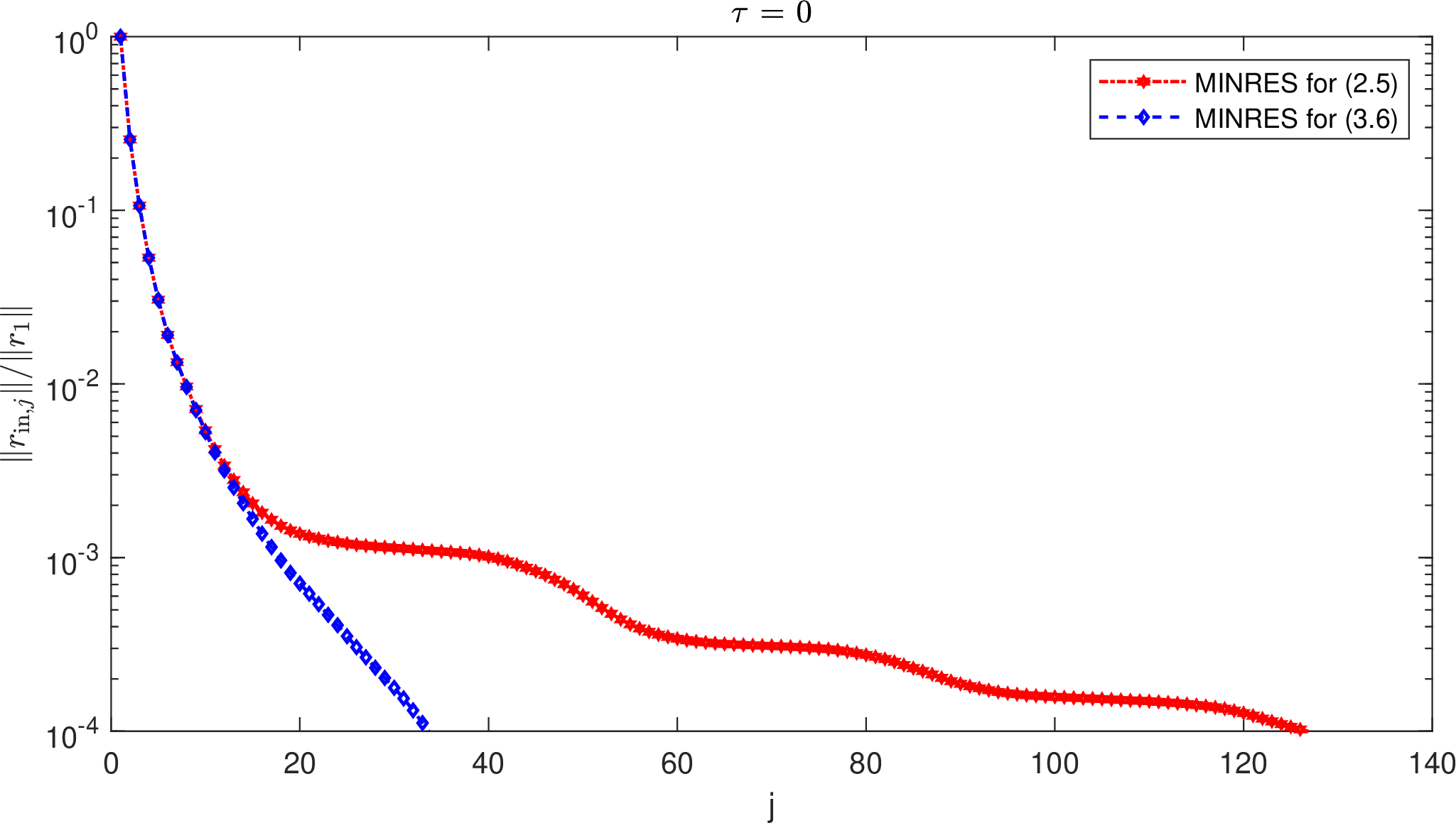
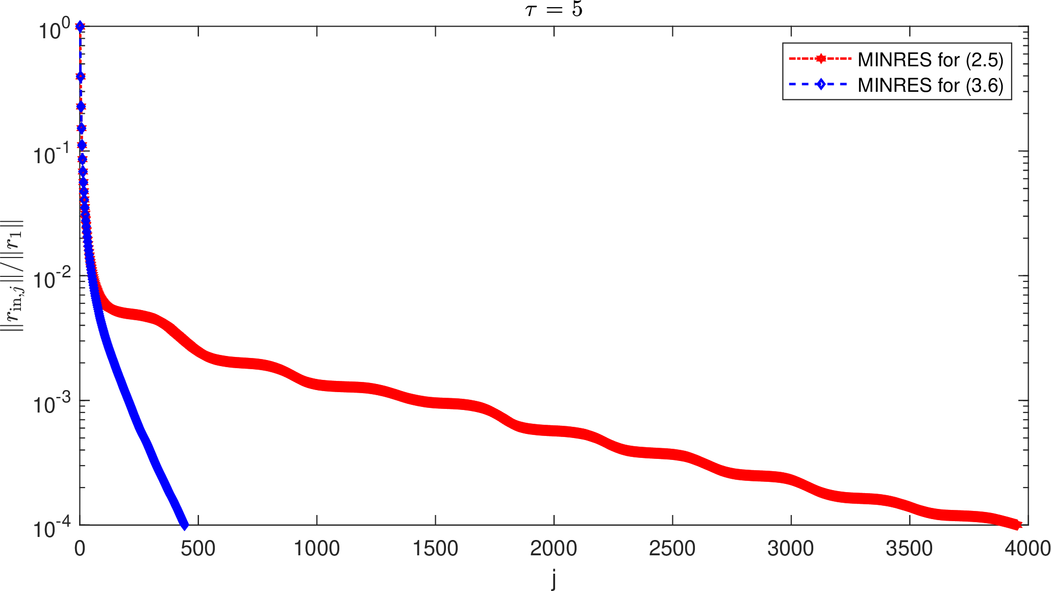
Figure 1: Convergence curves of MINRES for solving 7 and 15 ..
Notably, Theorem 4 characterizes the worst-case convergence behavior of MINRES for 15 and 7 . As illustrated in the figure, while MINRES exhibits comparable initial convergence for both equations, it ultimately converges significantly faster for 15 . As a consequence, to achieve a moderate relative residual tolerance of \(10^{-4}\), solving 15 requires only 26.19% and 11.18% of the iterations needed for 7 when \(\tau=0\) and \(5\), respectively.
When computing the largest, smallest, or an interior eigenvalue of \(A\) (corresponding to the cases \(\tau\approx\lambda_{\max}\), \(\lambda_{\min}\) and \(\lambda_{1}\), respectively), assuming \(\delta_m\) is sufficiently small, the parameters in 27 satisfy \[\small \gamma_1^{\prime}\approx\frac{\lambda_{\max}-\lambda_{\max,m+1}}{\lambda_{\max}-\lambda_{\min}},\qquad \gamma_2^{\prime}\approx\frac{\lambda_{\min,m+1}-\lambda_{\min}}{\lambda_{\max}-\lambda_{\min}},\qquad \gamma_3^{\prime}\approx\frac{|\lambda_{m+1}-\lambda_{1}|}{|\lambda_{n}-\lambda_{1}|}.\] Utilizing \(\frac{1}{2}(\lambda_{\max}-\lambda_{\min})\leq |\lambda_{n}-\lambda_{1}|\leq \lambda_{\max}-\lambda_{\min}\), we deduce \(\frac{\gamma_3^{\prime}}{2}\lessapprox\gamma_1^{\prime}\approx\gamma_2^{\prime}\lessapprox\gamma_3^{\prime}\) provided that \(\lambda_{\max}-\lambda_{\max,m+1}\approx\lambda_{\min,m+1}-\lambda_{\min}\approx |\lambda_{m+1}-\lambda_{1}|\). Given that \(\gamma_1^{\prime}, \gamma_2^{\prime},\gamma_3^{\prime}\) are typically smaller than \(1\), we have \(\gamma_3^{\prime}\lessapprox 2 \gamma_1^{\prime} < \frac{2\sqrt{\gamma_1^{\prime}}}{1+\gamma_1^{\prime}}\) and \(\gamma_3^{\prime}\lessapprox 2 \gamma_2^{\prime} < \frac{2\sqrt{\gamma_2^{\prime}}}{1+\gamma_2^{\prime}}\). Therefore, the theoretical convergence factors in ?? –?? satisfy \[1-\frac{2\sqrt{\gamma_1^{\prime}}}{1+\sqrt{\gamma_1^{\prime}}}\approx 1-\frac{2\sqrt{\gamma_2^{\prime}}}{1+\sqrt{\gamma_2^{\prime}}} < \left(1-\frac{2\gamma_3^{\prime}}{1+\gamma_3^{\prime}}\right)^{\frac{1}{2}}.\] This indicates that MINRES for 15 generally converges significantly faster for extreme eigenpairs than for interior ones, as fully corroborated by Figure 1.
3.3 Construction of new correction equations↩︎
The preceding analysis highlights the advantages of employing MINRES to solve the proposed correction equation 15 over the standard 7 , especially when \(A\) has a cluster of eigenvalues near \(\tau\) and sufficiently accurate approximations to the associated eigenvectors are available during the extraction phase. From a computational standpoint, it remains to establish rigorous numerical criteria for determining the cluster size \(m\), adaptively construct 15 , and develop a practical JD-V algorithm.
Given a reasonably small tolerance \(\epsilon_1>0\), an eigenvalue \(\lambda_i\) of \(A\) is classified as being clustered near the target \(\tau\) if \[\label{pretol1} |\lambda_i-\tau|\leq\max\{|\tau|,1\}\cdot\epsilon_1.\tag{28}\] By 10 , \(m\) is uniquely defined with \(|\lambda_{m}-\tau| \leq \max\{|\tau|,1\} \cdot \epsilon_1 <|\lambda_{m+1}-\tau|\). At the \(k\)th outer iteration of JD-V, we identify a Ritz value \(\theta_i\) (\(i=2,\dots,k\)) obtained from 4 –5 as an approximation to a clustered eigenvalue if \[\label{select1} |\theta_i-\tau|\leq\max\{|\tau|,1\}\cdot\epsilon_1.\tag{29}\]
Recall from section 3.1 that for 15 and 7 to yield equally effective subspace expansions, the higher order term \(R_{2:m}\widetilde{X}_{2:m}^*t\) omitted from 13 must be negligible compared to \(-r_1\). In light of 14 , this requires the block residual \(R_{2:m}\) to be sufficiently small. Furthermore, Theorem 4 dictates that for the theoretical bounds ?? –?? to be meaningful, and for MINRES to converge significantly faster for 15 than for 7 , the parameter \(\delta_m\) defined in ?? must be adequately small. Together, these conditions imply that the approximate eigenvectors \(\tilde{x}_2,\dots,\tilde{x}_m\) participating in 15 must have at least moderate accuracy. Therefore, if the residual \(r_i\) defined in 3 of a Ritz pair \((\theta_i,\tilde{x}_i)\) satisfies \[\label{select2} \|r_i\|\leq\|A\|_1 \cdot\epsilon_2,\tag{30}\] for a moderately small threshold \(\epsilon_2\), we accept \((\theta_i,\tilde{x}_i)\) as a reliable approximation to an eigenpair of \(A\). In practice, it suffices to employ \(\epsilon_2\gg \varepsilon_{\mathrm{out}}\), the outer stopping tolerance \(\varepsilon_{\mathrm{out}}\) in 6 . For example, when \(\varepsilon_{\mathrm{out}}\in[10^{-14},10^{-8}]\), numerical experiments indicate that \(\epsilon_2\in[10^{-3},10^{-2}]\) serves as a robust practical choice.
Assuming that there are \(\widetilde{m}-1\) indices \(i_2,\dots,i_{\widetilde{m}}\) from \(2,\dots,k\) fulfilling both 29 and 30 , we construct \[\label{tildeX} \widetilde{X}_{\widetilde{m}}= [\tilde{x}_1,\tilde{x}_{i_2},\dots,\tilde{x}_{i_{\widetilde{m}}}],\tag{31}\] and replace \(\widetilde{X}_m\) with \(\widetilde{X}_{\widetilde{m}}\) when forming 15 .
For a fixed \(\epsilon_2\gg\varepsilon_{\mathrm{out}}\), the selected approximate eigenvectors \(\tilde{x}_{i_2},\dots\), \(\tilde{x}_{i_{\widetilde{m}}}\) may have poorer accuracy than \(\tilde{x}_1\) as the outer iterations proceed, particularly when \(\varepsilon_{\mathrm{out}}<\frac{\|r_1\|}{\|A\|_1} \ll \frac{\|r_i\|}{\|A\|_1}\leq\epsilon_2\) for some \(i\in\{i_2,\dots,i_{\widetilde{m}}\}\). In this case, \(\|R_{i_2:i_{\widetilde{m}}}\|\) can significantly exceed \(\|r_1\|\). Consequently, omitting \(R_{i_2:i_{\widetilde{m}}}\widetilde{X}_{i_2:i_{\widetilde{m}}}^*t\) from 13 renders the solution to the resulting correction equation 15 marginally less effective in expanding subspace than that of 7 . As a result, JD-V may converge slightly slower than JD, as demonstrated in Figure 2. As a part of Experiment [exper1], the figure plots the outer convergence histories of both methods for computing the largest (left), smallest (middle), and an interior (right) eigenpair of the “barth” matrix from the SuiteSparse Matrix Collection [22], using the shifts \(\tau=7.4\), \(-2.3\), and \(0\), respectively. Ultimately, such a marginal delay in outer convergence is acceptable, given that the overall efficiency is substantially improved.
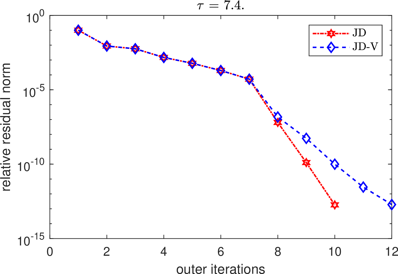
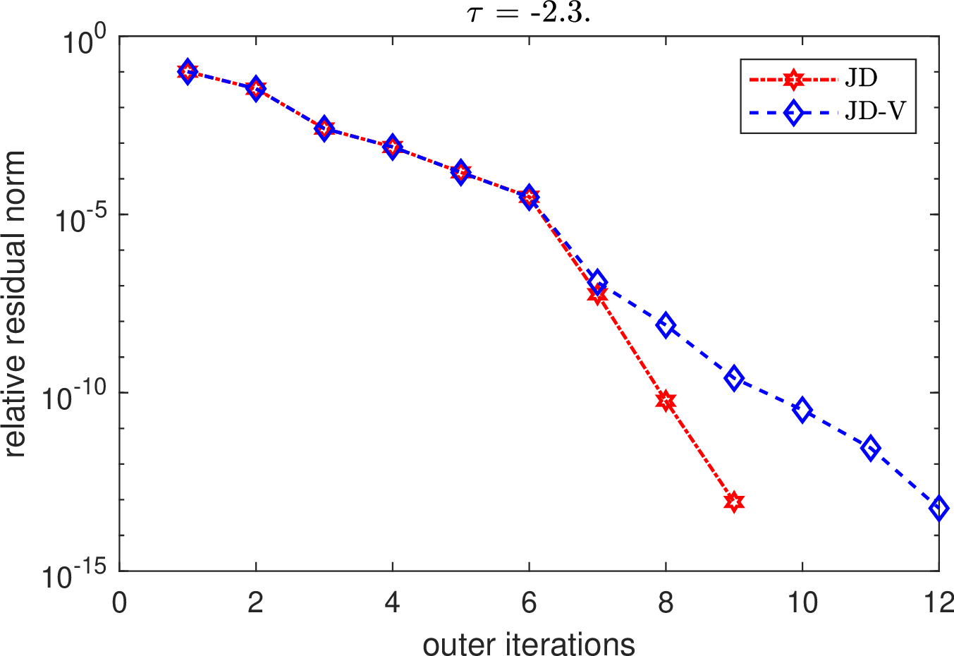
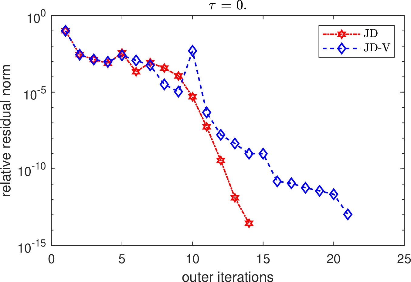
Figure 2: Computing one eigenpair of “barth” using JD-V and JD..
Given \(\epsilon_2>\varepsilon_{\mathrm{out}}\), the choice of \(\epsilon_1>0\) is critical. While a larger \(\epsilon_1\) expands the cluster size \(\widetilde{m}\) in 31 and accelerates MINRES convergence for 15 , it simultaneously increases the cost of matrix-vector multiplications involving the coefficient matrix \(\widetilde{B}_{\widetilde{m}}\) per MINRES iteration, particularly for sparse \(A\). To balance this trade-off, we empirically recommend choosing \(\epsilon_1\in[0.01, 0.05]\).
Two extreme cases are \(\epsilon_1=\epsilon_2=0\) and \(\epsilon_1=\epsilon_2=+\infty\). In the first case, \(\widetilde{m}\equiv m\equiv1\), and JD-V reduces to the standard JD method. In the second case, \(\widetilde{m}=k\), meaning all Ritz vectors are incorporated into 15 . The latter approach, equivalent to the one in [19] and denoted as JD-V(\(+\infty\)) hereafter, is known to be computationally inefficient [19], [23]. This inefficiency arises because the entire subspace \(\mathop{\mathrm{span}}\{\widetilde{X}_k\}\) is typically a poor approximation to any eigenspace of \(A\). Hence, \(R_{2:k}\widetilde{X}_{2:k}^*t\) dominates \(-r_1\) in 13 , causing the solution of the relevant correction equation 15 to deviate significantly from the standard correction 7 . As a result, JD-V(\(+\infty\)) expands the subspace ineffectively and demands significantly more outer iterations to converge than the standard JD and JD-V, a phenomenon confirmed numerically in Experiments [exper1]–[exper2].
For \(k\) small, there maybe no Ritz pair satisfy 29 –30 . In this case, \(\widetilde{m}=1\), and 15 reduces to the standard 7 . Nevertheless, for \(m>1\), as \(k\) grows, more Ritz pairs begin to satisfy these criteria. Consequently, incorporating multiple Ritz vectors (\(\widetilde{m}>1\)) into 15 enables JD-V to outperform JD in overall efficiency. Ultimately, \(\widetilde{m}\) reaches \(m\) as JD-V approaches convergence.
4 A thick-restart JD-V algorithm with deflation and purgation↩︎
To compute \(\ell>1\) eigenpairs of \(A\) near \(\tau\), we propose an efficient thick-restart JD-V algorithm incorporating adaptive shifts, deflation, and purgation.
4.1 Thick restart↩︎
For practical purpose, we adapt the thick-restart strategy introduced in [18] for JDSVD-V method to the JD-V algorithm.
Specifically, given the user-prescribed maximum and minimum subspace dimensions \(k_{\max}\) and \(k_{\min}\), when \(k=k_{\max}\), we retain a restarting subspace \(\mathcal{X}_{\mathop{\mathrm{new}}}\subset \mathcal{X}\) of dimension \[k_{\mathop{\mathrm{new}}}=\max\{k_{\min},\widetilde{m}\},\] where \(\widetilde{m}\) is as in 31 . The orthonormal basis matrix \(\widetilde{X}\) of \(\mathcal{X}_{\mathop{\mathrm{new}}}\) and the associated projected matrix \(H\) are updated as follows:
If \(\widetilde{m}<k_{\min}\), we set \(\widetilde{X}=[\tilde{x}_1,\dots,\tilde{x}_{k_{\min}}]\) and \(H=\mathop{\mathrm{diag}}\{\theta_1,\dots,\theta_{k_{\min}}\}\);
If \(\widetilde{m}\geq k_{\min}\), then \(\widetilde{X}=[\tilde{x}_1,\tilde{x}_{i_2},\dots,\tilde{x}_{i_{\widetilde{m}}}]\) and \(H=\mathop{\mathrm{diag}}\{\theta_1,\theta_{i_2},\dots,\theta_{i_{\widetilde{m}}}\}\).
Initially, when \(\widetilde{m}<k_{\min}\), the restarting subspace \(\mathcal{X}_{\mathop{\mathrm{new}}}\) is spanned by the \(k_{\min}\) Ritz vectors associated with the Ritz values closest to \(\tau\). As the iterations proceed and \(\widetilde{m}\geq k_{\min}\), \(\mathcal{X}_{\mathop{\mathrm{new}}}\) adaptively retains all sufficiently accurate Ritz vectors within the target cluster. Consequently, for \(k_{\min}<m\ll k_{\max}\), the thick-restart JD-V algorithm requires substantially fewer outer iterations than the conventional scheme with a fixed restart dimension \(k_{\mathop{\mathrm{new}}}\equiv k_{\min}\).
4.2 Deflation↩︎
The JD-V method naturally incorporates deflation when computing several eigenpairs \((\lambda_i, x_i)\), \(i=1, \dots, \ell\) closest to the target \(\tau\).
Assume that \(\ell_{\mathrm{c}}<\ell\) approximate eigenpairs \((\theta_{1,\mathrm{c}},\tilde{x}_{1,\mathrm{c}}),\dots, (\theta_{\ell_{\mathrm{c}},\mathrm{c}}, \tilde{x}_{\ell_{\mathrm{c}}, \mathrm{c}})\) have converged to the desired \((\lambda_1,x_1)\), \(\dots\), \((\lambda_{\ell_{\mathrm{c}}},x_{\ell_{\mathrm{c}}})\), with the approximate eigenvectors mutually orthonormal. Here, the subscript “\(\mathrm{c}\)” indicates converged quantities. Then \[\label{convergRitz} (\Lambda_{\mathrm{c}},X_{\mathrm{c}})= (\mathop{\mathrm{diag}}\{\theta_{1,\mathrm{c}},\dots,\theta_{\ell_{\mathrm{c}},\mathrm{c}}\}, [\tilde{x}_{1,\mathrm{c}},\dots,\tilde{x}_{\ell_{\mathrm{c}},\mathrm{c}}])\tag{32}\] is a converged approximation to the block eigenpair \((\Lambda_{\ell_{\mathrm{c}}}, X_{\ell_{\mathrm{c}}})\) of \(A\); see 11 . By definition, the next desired \((\lambda_{\ell_{\mathrm{c}}+1},x_{\ell_{\mathrm{c}}+1})\) is an eigenpair of \((I-X_{\ell_{\mathrm{c}}}X_{\ell_{\mathrm{c}}}^*) A(I-X_{\ell_{\mathrm{c}}}X_{\ell_{\mathrm{c}}}^*)\) restricted to \(X_{\ell_{\mathrm{c}}}^{\perp}\) with the eigenvalue closest to \(\tau\). By a continuity argument, we can apply JD-V to \(\widetilde{A} = (I-X_{\mathrm{c}}X_{\mathrm{c}}^*)A(I-X_{\mathrm{c}}X_{\mathrm{c}}^*)\) restricted to \(X_{\mathrm{c}}^{\perp}\) to compute it.
By enforcing the search subspace \(\mathcal{X}\perp \mathop{\mathrm{span}}\{X_{\mathrm{c}}\}\), the extraction phase of the deflated JD-V method remains identical to that in section 2. We take the Ritz pair \((\theta_1,\tilde{x}_1)\) from 5 as an approximate to the desired \((\lambda_{\ell_{\mathrm{c}}+1},x_{\ell_{\mathrm{c}}+1})\). The corresponding residuals with respect to the eigenproblems of \(A\) and \(\widetilde{A}|_{X_{\mathrm{c}}^{\perp}}\) are \(r_1\) in 3 and \(\tilde{r}_1=(I-X_{\mathrm{c}}X_{\mathrm{c}}^*)r_1\), respectively. If \((\theta_1,\tilde{x}_1)\) has not yet converged according to 6 , we determine the \(\widetilde{m}-1\) indices \(i_2,\dots,i_{\widetilde{m}}\) based on 29 –30 , and construct \(\widetilde{X}_{\widetilde{m}}\) via 31 . We then employ MINRES to solve the modified correction equation 15 , replacing \(A\) and \(r_1\) with \(\widetilde{A}\) and \(\tilde{r}_1\), respectively. Since \(\tilde{x}_i\in\mathcal{X}\perp\mathop{\mathrm{span}}\{X_{\mathrm{c}}\}\) for all \(i=1,\dots,k\), the deflated JD-V correction equation takes the form \[\label{correctionc} (I-\widetilde{X}_{\mathrm{d}}\widetilde{X}_{\mathrm{d}}^*) (A-\tau I)(I-\widetilde{X}_{\mathrm{d}}\widetilde{X}_{\mathrm{d}}^*) t = -\tilde{r}_1 \quadwith\quad t\perp \widetilde{X}_{\mathrm{d}}=[X_{\mathrm{c}},\widetilde{X}_{\widetilde{m}}],\tag{33}\] where the subscript “\(\mathrm{d}\)” denotes deflation. We terminate the inner MINRES iterations for solving 33 when the inner residual \(r_{\mathrm{in}}\) satisfies \[\label{innstop} \|r_{\mathrm{in}}\|\leq \|\tilde{r}_{1}\| \cdot \min\{\beta \varepsilon_{\mathrm{in}},0.1\},\tag{34}\] where \(\beta\) depends on the current Ritz values, and the threshold \(\varepsilon_{\mathrm{in}}\in[10^{-4},10^{-3}]\); see [15], [16]. We then use the approximate solution \(\tilde{t}\) to expand the search subspace: \(\mathcal{X}_{\mathop{\mathrm{new}}}=\mathop{\mathrm{span}}\{\mathcal{X},\tilde{t}\}\), which is inherently orthogonal to \(\mathop{\mathrm{span}}\{X_{\mathrm{c}}\}\) since both \(\tilde{t}\) and \(\mathcal{X}\) are so. New Ritz pairs are then extracted from \(\mathcal{X}_{\mathop{\mathrm{new}}}\) until \((\theta_1,\tilde{x}_1)\) converges.
Upon convergence, we assign \((\theta_{\ell_{\mathrm{c}}+1,\mathrm{c}},\tilde{x}_{\ell_{\mathrm{c}}+1,\mathrm{c}}) =(\theta_1,\tilde{x}_1)\), append it to the converged block eigenpair \((\Lambda_{\mathrm{c}},X_{\mathrm{c}}) =(\mathop{\mathrm{diag}}\{\Lambda_{\mathrm{c}},\theta_{\ell_{\mathrm{c}}+1,\mathrm{c}} \}, [X_{\mathrm{c}},\tilde{x}_{\ell_{\mathrm{c}}+1,\mathrm{c}}])\), and increment \(\ell_{\mathrm{c}}\) by \(1\). Repeat until all \(\ell\) desired eigenpairs of \(A\) are computed.
4.3 Purgation↩︎
When computing \((\lambda_{\ell_{\mathrm{c}}+1}, x_{\ell_{\mathrm{c}}+1})\) for \(\ell_{\mathrm{c}}\geq 1\), the search subspace \(\mathcal{X}\) from the preceding convergence cycle for \((\lambda_{\ell_{\mathrm{c}}},x_{\ell_{\mathrm{c}}})\) typically retains rich information about \(x_{\ell_{\mathrm{c}}+1}\). Rather than initializing a new subspace from scratch, we purge the recently converged Ritz vector \(\tilde{x}_{1}=\tilde{x}_{\ell_{\mathrm{c}},\mathrm{c}}\) from \(\mathcal{X}\), and employ the reduced subspace \(\mathcal{X}_{\mathop{\mathrm{new}}}=\mathop{\mathrm{span}}\{\tilde{x}_2,\dots,\tilde{x}_{k}\}\) as the initial search subspace. Clearly, this \(\mathcal{X}_{\mathop{\mathrm{new}}}\) is inherently orthogonal to \(\mathop{\mathrm{span}}\{X_c\}\). An orthonormal basis for \(\mathcal{X}_{\mathop{\mathrm{new}}}\) and the corresponding projected matrix \(H\) are naturally given by \[\widetilde{X}=[\tilde{x}_2,\dots,\tilde{x}_{k}] \qquadand\qquad H= \mathop{\mathrm{diag}}\{\theta_2,\dots,\theta_k\}.\] Referred to as purgation [17], this technique leverages the reduced subspace to substantially reduce the total number of outer iterations required for computing the \(2\)nd through \(\ell\)th eigenpairs.
4.4 Adaptively changing shift↩︎
As \(\ell_{\mathrm{c}}\) increases, the deflated operator \(\widetilde{A}|_{\widetilde{X}_{\mathrm{c}}^{\perp}}\) has \(m-\ell_{\mathrm{c}}\) clustered eigenvalues near \(\tau\) (i.e., \(\lambda_{\ell_{\mathrm{c}}+1},\dots,\lambda_{m}\)), dictating \(1\leq \widetilde{m}\leq m-\ell_{\mathrm{c}}\) for \(\ell_{\mathrm{c}}<m\). When \(\ell_{\mathrm{c}}\geq m\), we have \(\widetilde{m}\equiv1\), which reduces 33 to the standard deflated correction equation, and simplifies JD-V to JD. While this enables rapid MINRES convergence, the outer iterations often converge slowly. To accelerate outer convergence and enhance overall efficiency, we substitute the target \(\tau\) in 33 with a dynamic shift \(\theta_1\) once it is sufficiently accurate. Specifically, when \[\label{switch} \|r_1\|\leq \|A\|_1 \cdot \varepsilon_{\mathrm{\tau}}\tag{35}\] for a user-prescribed tolerance \(\varepsilon_{\mathrm{\tau}} >\varepsilon_{\mathrm{out}}\), we form \(\widetilde{X}_{\widetilde{m}}=[x_1,x_{i_2},\dots,x_{i_{\widetilde{m}}}]\) with the indices \(i_2,\dots,i_{\widetilde{m}}\) determined via 29 –30 by replacing \(\tau\) with \(\theta_1\). The deflated correction equation with this adaptive shift then becomes \[\label{correctiont} (I-\widetilde{X}_{\mathrm{d}}\widetilde{X}_{\mathrm{d}}^*) (A-\theta_1 I)(I-\widetilde{X}_{\mathrm{d}}\widetilde{X}_{\mathrm{d}}^*) t = -\tilde{r}_{1} \quadwith\quad t\perp \widetilde{X}_{\mathrm{d}}.\tag{36}\]
The convergence theory established in section 3.2 applies to 36 by replacing \(\tau\) with \(\theta_1\), implying that MINRES converges substantially faster for 36 than for the fixed-shift equation 33 , provided that the desired eigenvalue \(\lambda_{\ell_{\mathrm{c}}+1}\) is well separated from \(\lambda_1,\dots,\lambda_{\ell_{\mathrm{c}}}\), yet tightly clustered with the remaining eigenvalues of \(A\).
4.5 Thick-restart JD-V with deflation and purgation, a pseudocode↩︎
Algorithm 3 sketches the thick-restart JD-V algorithm with deflation and purgation.
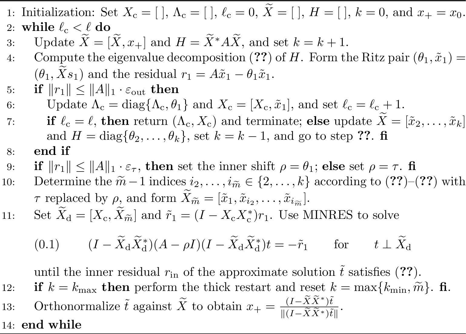
To reduce computational costs during the extraction phase, we do not explicitly evaluate all Ritz pairs and their residuals. Rather, we selectively compute those associated with the principal Ritz value \(\theta_1\) at Step [step], and those with Ritz values nearest to the inner shift \(\rho=\tau\) or \(\theta_1\) at Step [step3]. As the eigenpairs of the diagonal matrix \(H\) are trivially known when turning from step [step2] to step [step], it is sufficient to compute the residual \(r_1\) for the target pair \((\theta_1,\tilde{x}_1)\). In step [step4], solving [correctionfinal] via MINRES involves matrix-vector multiplications between the coefficient matrix \(\widetilde{B}_{\widetilde{m}+\ell_{\mathrm{c}}}\) and vectors \(\bar t\in\mathcal{K}_j(B_{\widetilde{m}+\ell_{\mathrm{c}}},\tilde{r}_1)\) for \(j\geq1\). Clearly, \(\widetilde{B}_{\widetilde{m}+\ell_{\mathrm{c}}}\bar t=\widehat B_{\widetilde{m}+\ell_{\mathrm{c}}}\bar t\) with \[\widehat B_{\widetilde{m}+\ell_{\mathrm{c}}} = (I-\widetilde{X}_{\mathrm{d}}\widetilde{X}_{\mathrm{d}}^*) (A-\rho I).\] Therefore, we equivalently apply the one-sided projected matrix \(\widehat B_{\widetilde{m}+\ell_{\mathrm{c}}}\) at each MINRES step, which is substantially more efficient than applying the two-sided projection \(\widetilde{B}_{\widetilde{m}+\ell_{\mathrm{c}}}\), especially when \(A\) is highly sparse and the dimension \(\widetilde{m}+\ell_{\mathrm{c}}\) is large.
Given a target \(\tau\), Algorithm 3 requires as inputs a routine for computing matrix-vector products with \(A\), the number \(\ell\) of desired eigenpairs, and the outer stopping tolerance \(\varepsilon_{\mathrm{out}}\) in 6 . Upon convergence, it outputs an approximate block eigenpair \((\Lambda_{\mathrm{c}},X_{\mathrm{c}})\) of size \(\ell\), with \(X_{\mathrm{c}}\) having orthonormal columns, satisfying \[\|AX_{\mathrm{c}}-X_{\mathrm{c}}\Lambda_{\mathrm{c}}\|_\mathrm{F} \leq\sqrt{\ell}\|A\|_1\cdot\varepsilon_{\mathrm{out}},\] where \(\|\cdot\|_\mathrm{F}\) denotes the Frobenius norm. Optional parameters include the normalized starting vector \(x_0\in\mathbb{C}^n\), the subspace dimension bounds \(k_{\max}\) and \(k_{\min}\), the inner stopping tolerance \(\varepsilon_{\mathrm{in}}\) in 34 , the threshold \(\varepsilon_{\tau}\) in 35 governing the transition from the fixed target \(\tau\) to the adaptive shift \(\theta_1\), and the clustering and accuracy tolerances \(\epsilon_1\) and \(\epsilon_2\) in 29 –30 . The default values are set as \(x_0=\frac{1}{\sqrt{n}}[1,\dots,1]^*\), \(k_{\max}=30\), \(k_{\min}=3\), \(\varepsilon_{\mathrm{in}}=10^{-3}\), \(\varepsilon_{\tau}=10^{-4}\) and \(\epsilon_1=0.05\), \(\epsilon_2=0.01\). Additionally, MINRES utilizes the zero vector as its initial guess when solving the correction equation [correctionfinal].
5 Numerical examples↩︎
We report numerical experiments on several test problems to illustrate the effectiveness and efficiency of the thick-restarted JD-V algorithm for computing several eigenpairs of a large Hermitian matrix \(A\) near \(\tau\). The algorithm was developed in MATLAB. All the experiments were implemented on an Intel (R) core (TM) i9-10885H CPU 2.40 GHz with the main memory 64 GB and 16 cores using the MATLAB R2021a with the machine precision \(\epsilon=2.22\times 10^{-16}\) under the Microsoft Windows 10 64-bit system.
Compute the \(20\) largest, smallest and interior clustered eigenpairs of the \(6691\times 6691\) sparse “barth” matrix (with \(46187\) nonzero entries) from the SuiteSparse Matrix Collection [22] using the unrestarted standard JD (\(\epsilon_1=\epsilon_2=0\)), JD-V (\(\epsilon_1=0.01\) and \(\epsilon_2=0.05\)) and JD-V(\(+\infty\)) (\(\epsilon_1=\epsilon_2=+\infty\)) algorithms, with the targets \(\tau=7.4\), \(-2.3\), and \(0\), respectively. Set the outer stopping tolerance to \(\varepsilon_{\mathrm{out}}=10^{-12}\), and keep all other parameters at their default values.
| \(\tau\) | JD | JD-V | JD-V(\(+\infty\)) | ||||||
|---|---|---|---|---|---|---|---|---|---|
| 2-4 (lr)5-7(lr)8-10 | \(i_{\mathrm{out}}\) | \(i_{\mathrm{in}}\) | time | \(i_{\mathrm{out}}\) | \(i_{\mathrm{in}}\) | time | \(i_{\mathrm{out}}\) | \(i_{\mathrm{in}}\) | time |
| 105 | 4584 | 0.73 | 129 | 3502 | 1.20 | 363 | 5263 | 9.76 | |
| -2.3 | 105 | 5653 | 0.82 | 126 | 4007 | 1.09 | 490 | 8877 | 18.9 |
| 0 | 121 | 520280 | 44.0 | 218 | 306181 | 32.3 | 251 | 316460 | 36.2 |
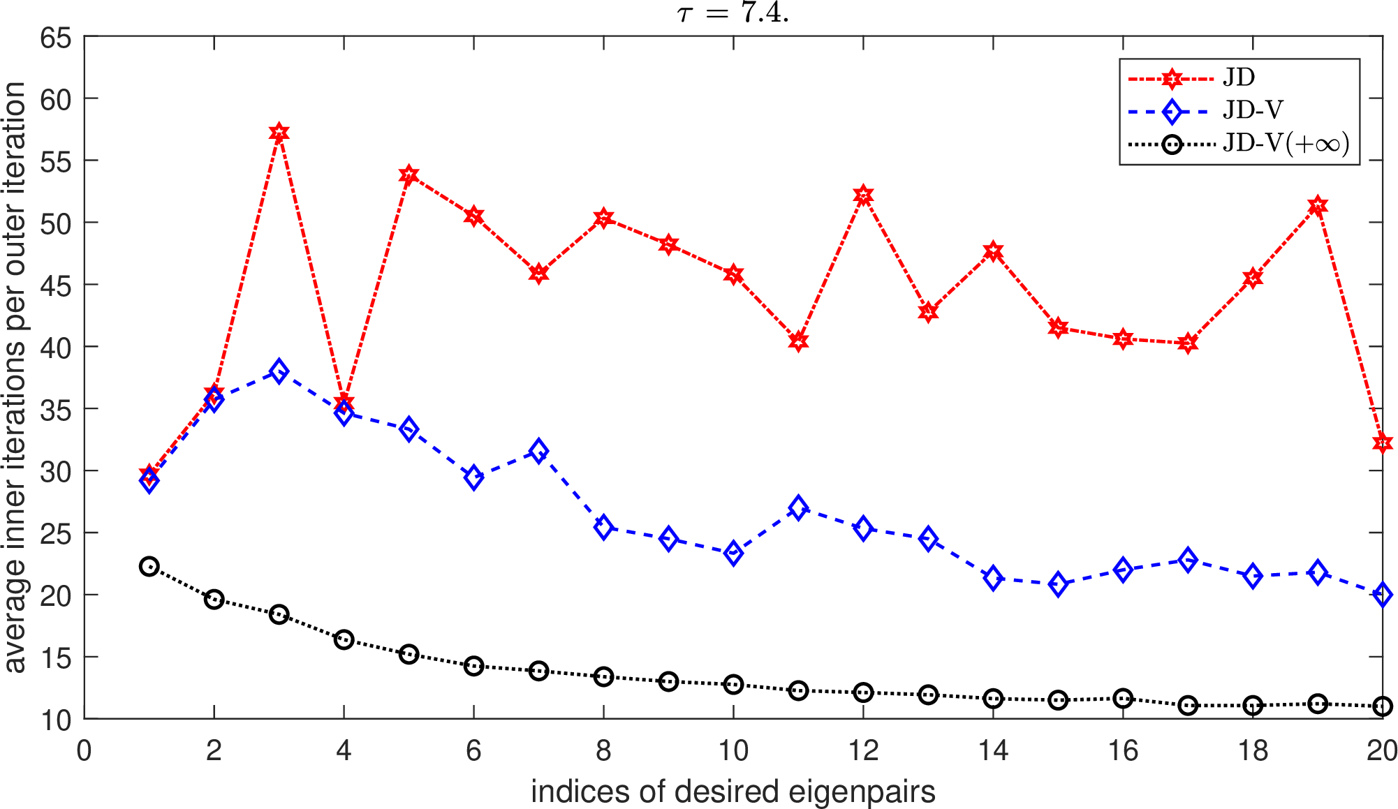
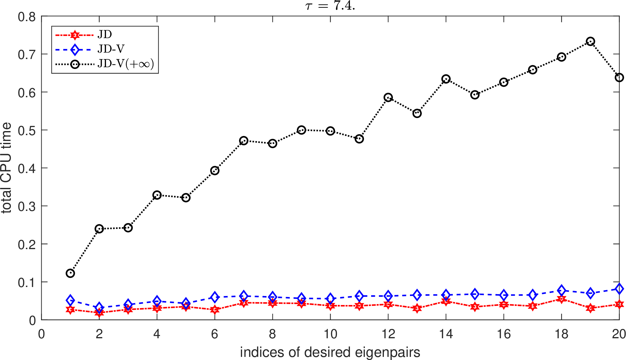
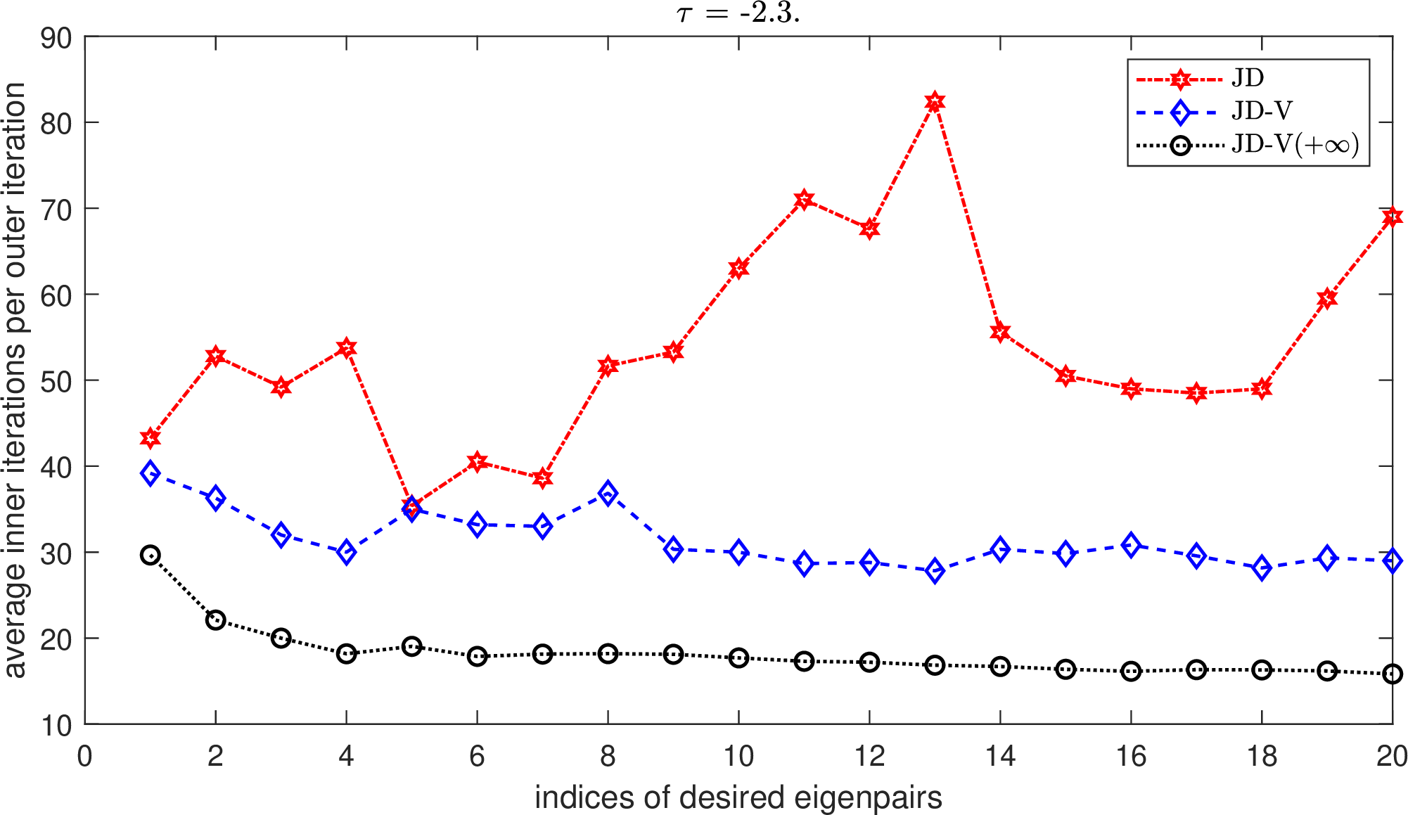
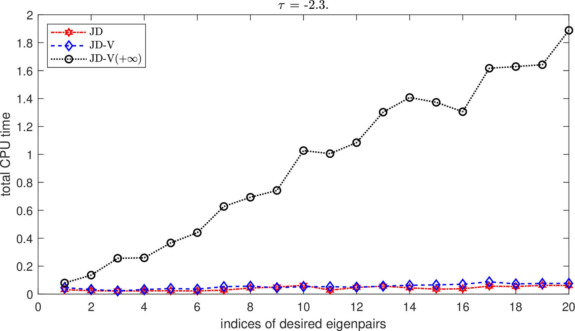
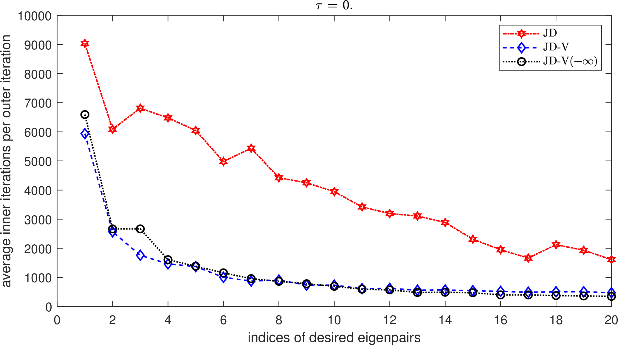
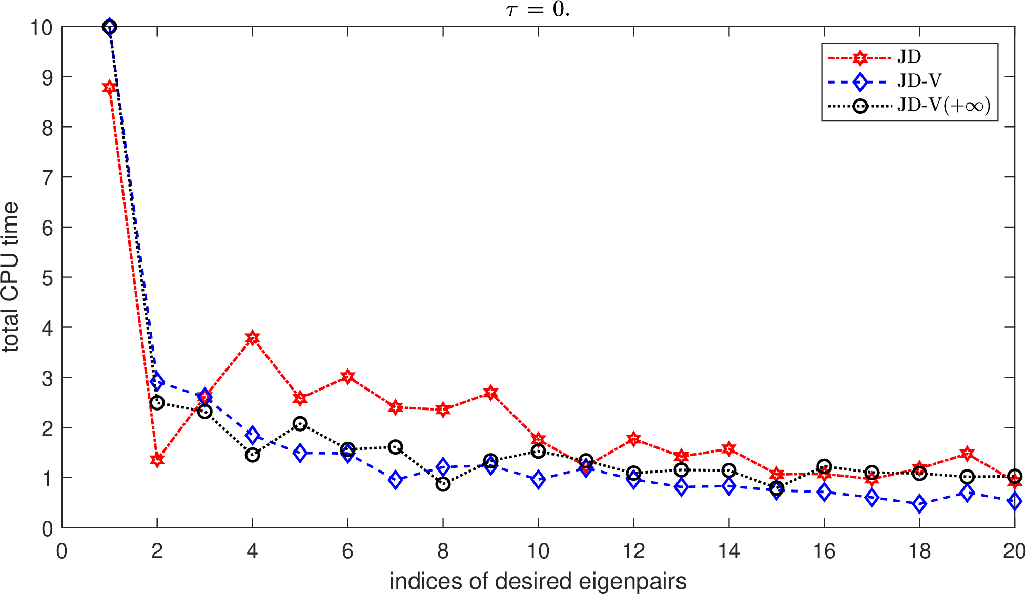
Figure 4: Computing \(20\) eigenpairs of “barth” using the unrestarted JD-type algorithms..
For each target, all three unrestarted algorithms successfully compute all the desired eigenpairs of \(A\). Table ¿tbl:table1a? reports the computational results, where \(i_{\mathrm{out}}\) and \(i_{\mathrm{in}}\) denote the total numbers of outer and inner iterations required for convergence, respectively; “time” represents the overall CPU time in seconds measured via the MATLAB timer; and boldface values indicate the optimal results. Figure 4 depicts the average number of inner iterations per outer iteration (left) and total CPU time (right) each algorithm used to compute each desired eigenpair.
As shown in Table ¿tbl:table1a?, for each \(\tau\), JD-V requires slightly or even considerably more outer iterations than JD, for the reasons detailed in Remark [remark9]. Nonetheless, it reduces the inner iterations of JD by 23.60%, 29.12%, and 41.15% when computing the largest, smallest, and interior eigenpairs, respectively, demonstrating that MINRES solves the correction equations in JD-V more efficiently than those JD, as corroborated by Figure 4 (left). Consequently, JD-V consumes moderately more CPU time than JD for the first two relatively straightforward problems. This is primarily attributed to the growing overhead of the extraction phase during outer iterations; for this moderately sized matrix, computing the spectral decomposition of the projected matrix becomes increasingly expensive as the search subspace expands. However, for the most challenging problem (\(\tau=0\)), JD-V reduces the CPU time by 26.59% compared to JD, confirming the efficacy of the proposed correction equations.
We see from Figure 4 that for most of the desired eigenpairs across all targets, JD-V(\(+\infty\)) requires fewer, and occasionally substantially fewer, inner iterations on average per outer iteration than both JD and JD-V. However, it suffers from a significantly higher number of outer iterations, driven by the factors explained in Remark [remark3]. As a result, the overall efficiency of JD-V(\(+\infty\)) remains considerably inferior to that of JD and JD-V in terms of both iteration counts and total CPU time.
Furthermore, we observe that for the highly challenging interior eigenvalue problem (\(\tau=0\)), each algorithm requires substantially fewer outer iterations to compute the subsequent eigenpairs than to compute the first one, validating the effectiveness of the purgation technique introduced in section 4.3. In addition, as illustrated in Figure 4, MINRES converges significantly faster on average for the second through last eigenpairs. This occurs because high-quality spectral information accumulates within the search subspace, which in turn leads to better-conditioned correction equations. As a result, all three algorithms consume substantially less CPU time computing the subsequent eigenpairs than the first one. Notably, for this problem, although JD-V uses more CPU time than JD to compute the first eigenpair due to more outer iterations, it ultimately achieves a lower total CPU time owing to the computational savings accrued during the computation of subsequent eigenpairs. This demonstrates that the advantages of JD-V over the standard JD become increasingly pronounced when multiple eigenpairs, rather than a single one, is computed.
Following the exact setup in Experiment [exper1], compute the \(20\) eigenpairs of \(A\) using the thick-restart JD, JD-V, and JD-V(\(+\infty\)) algorithms, with the search subspace dimension bounded by \(k_{\max}=30\) and \(k_{\min}=3\).
For each target, all three algorithms successfully compute the desired eigenpairs of \(A\), with the numerical results reported in Table ¿tbl:table1b? and Figure 5.
| \(\tau\) | JD | JD-V | JD-V(\(+\infty\)) | ||||||
|---|---|---|---|---|---|---|---|---|---|
| 2-4 (lr)5-7(lr)8-10 | \(i_{\mathrm{out}}\) | \(i_{\mathrm{in}}\) | time | \(i_{\mathrm{out}}\) | \(i_{\mathrm{in}}\) | time | \(i_{\mathrm{out}}\) | \(i_{\mathrm{in}}\) | time |
| 125 | 6269 | 0.74 | 123 | 3639 | 0.72 | 548 | 18066 | 2.97 | |
| -2.3 | 117 | 7092 | 0.79 | 132 | 4310 | 0.79 | 546 | 19844 | 3.17 |
| 0 | 119 | 601040 | 50.7 | 211 | 305923 | 31.5 | 413 | 1094717 | 102 |
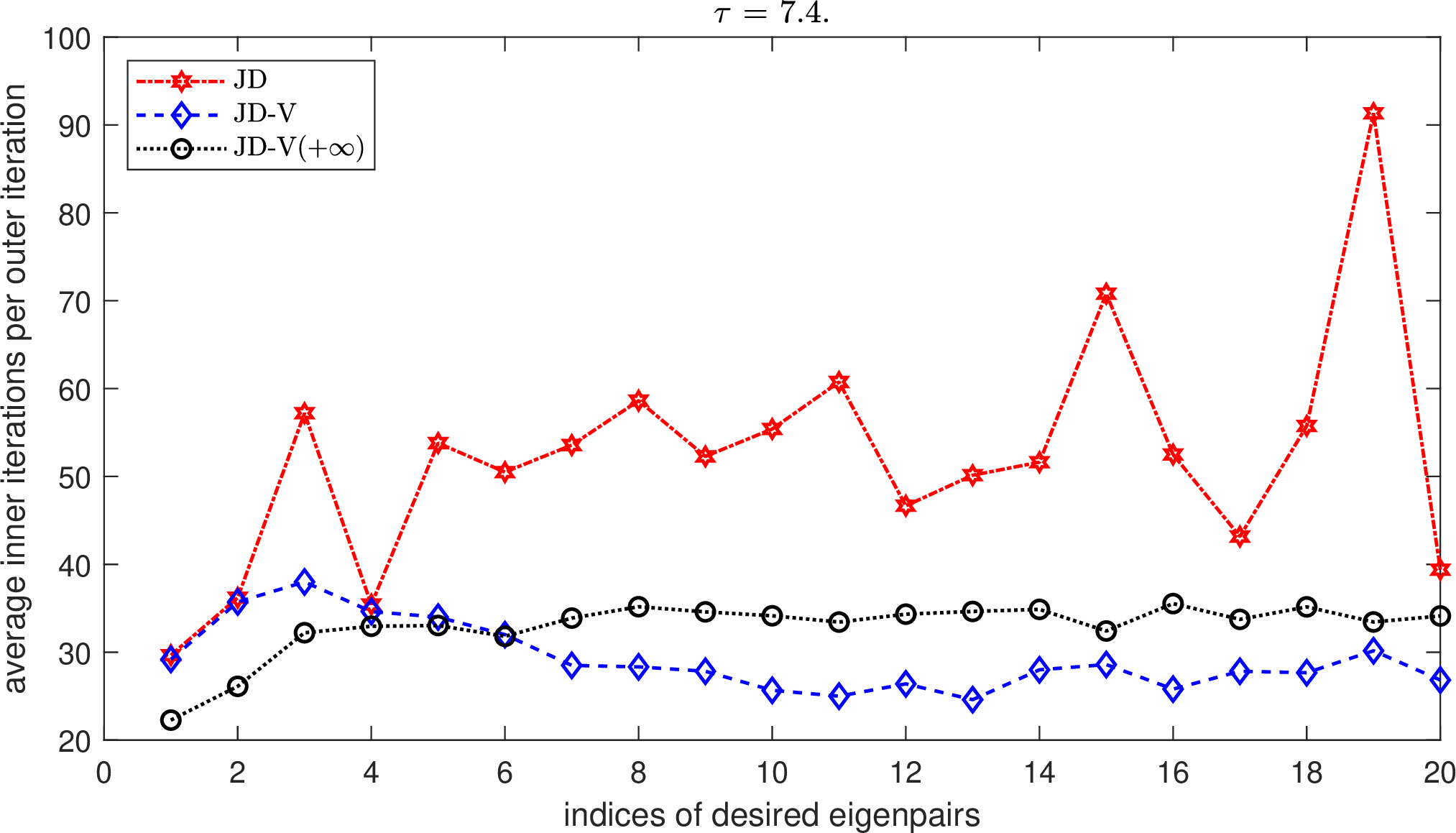
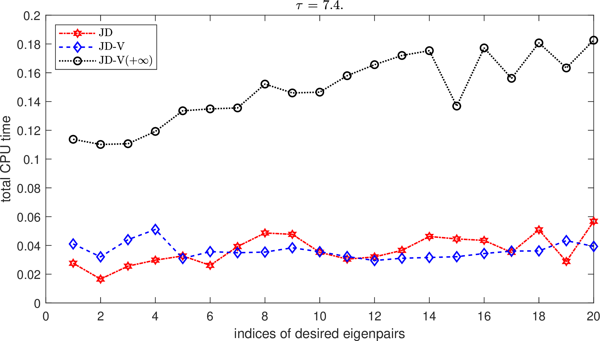
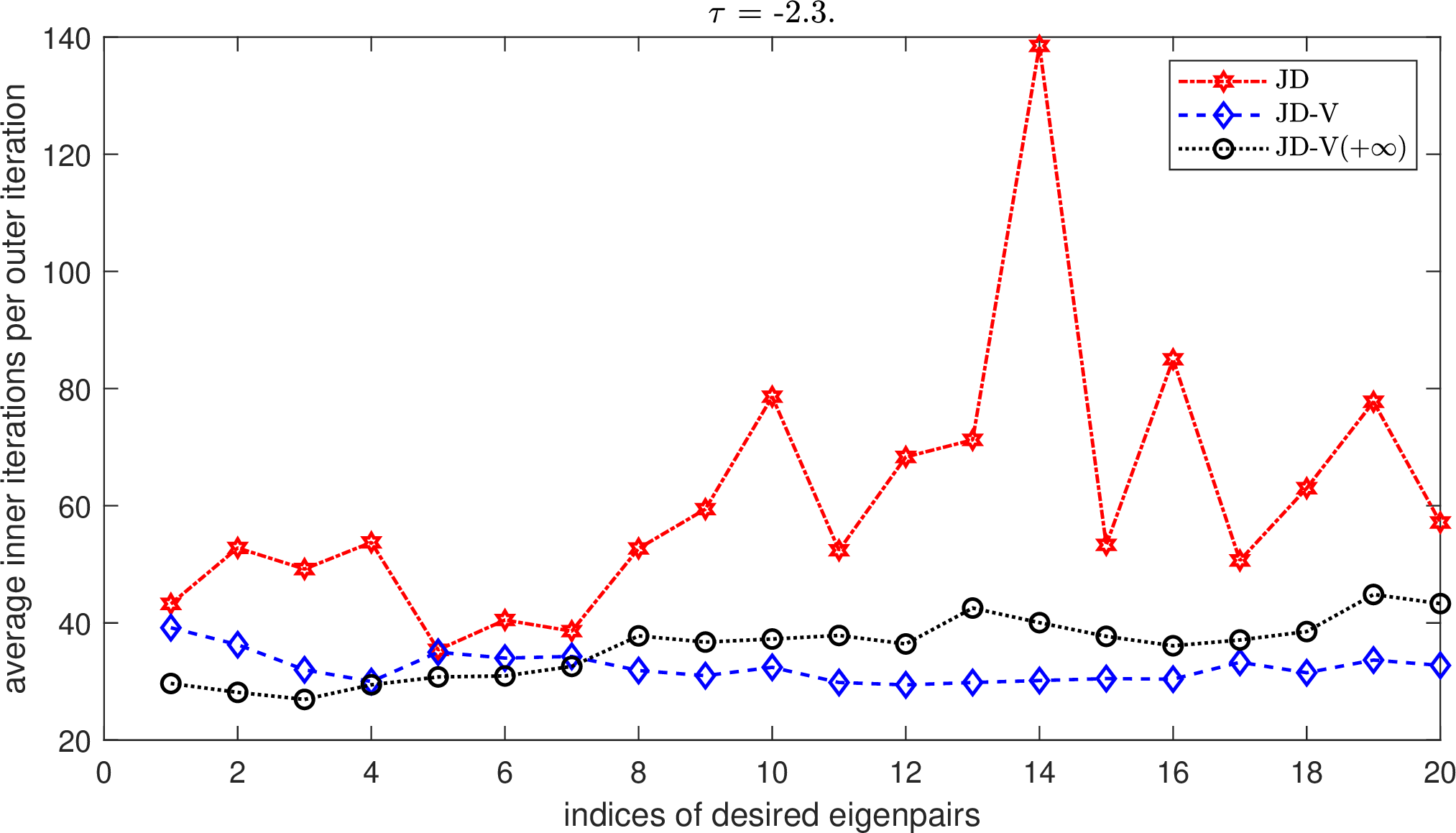

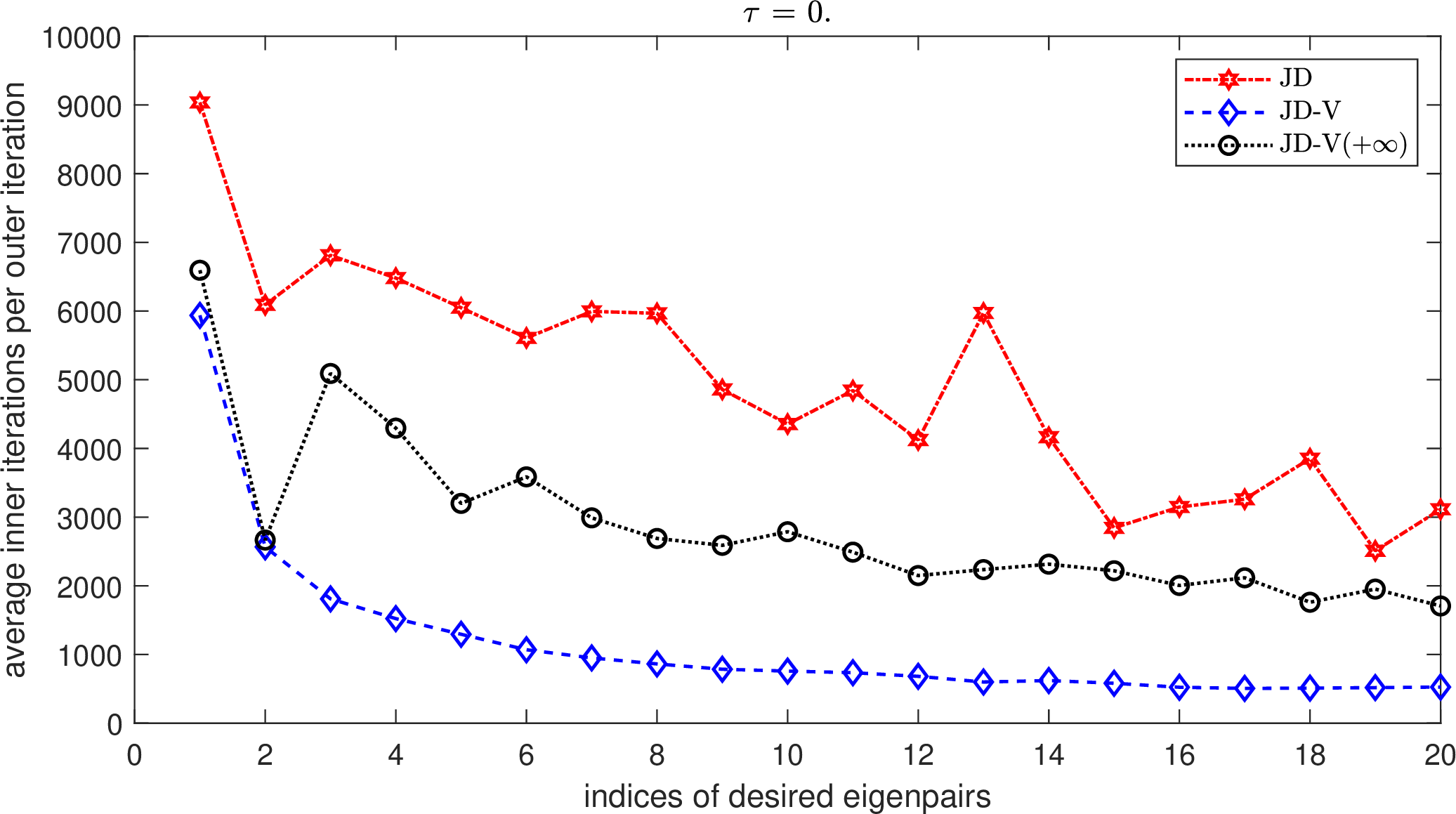
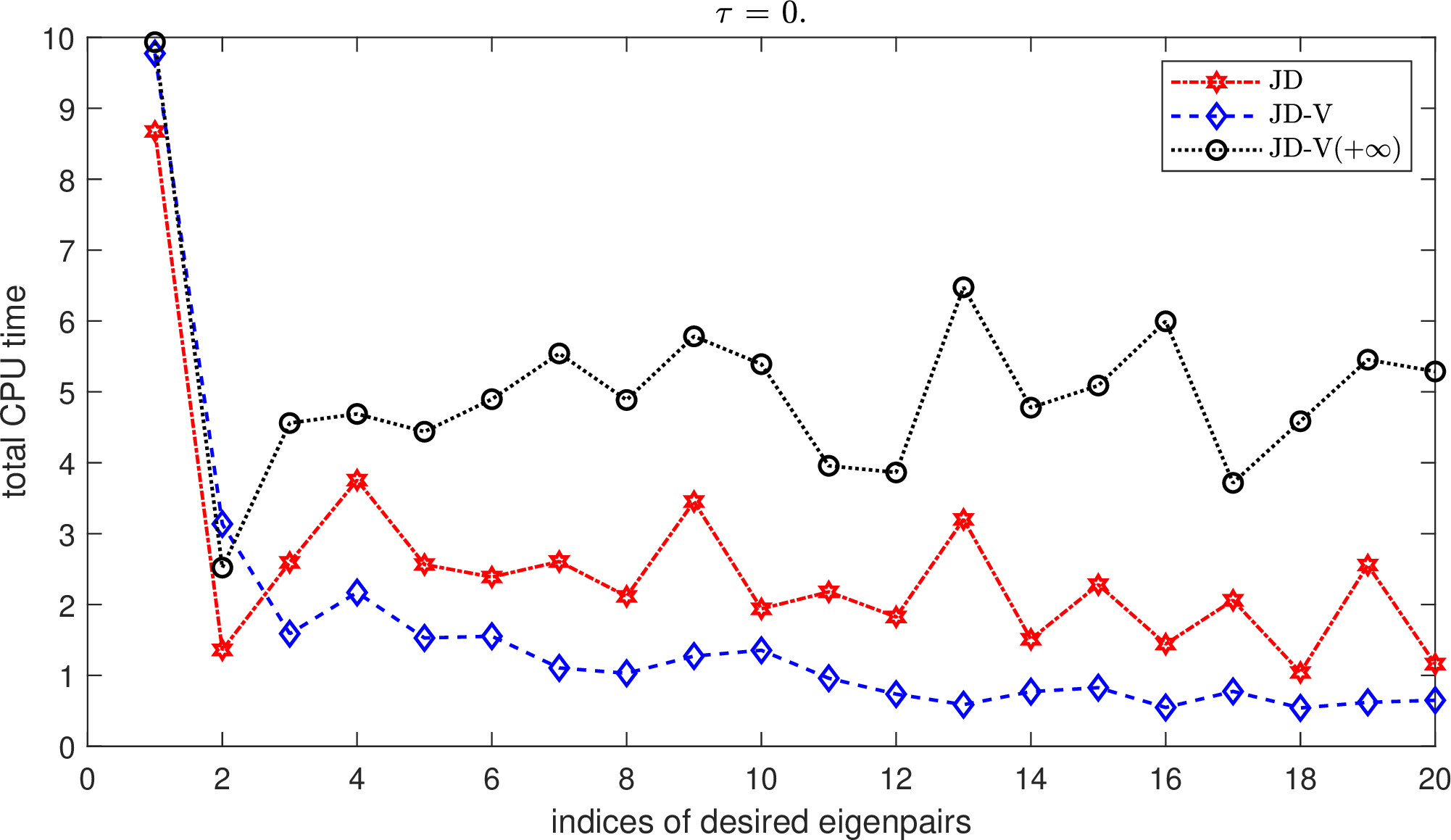
Figure 5: Computing 20 eigenpairs of “barth” using the thick-restart JD-type algorithms..
Comparing the results in Tables ¿tbl:table1a? and ¿tbl:table1b?, we observe that for most of the test problems, the thick-restart JD and JD-V(\(+\infty\)) algorithms requires more and, in some cases, substantially more outer iterations than their unrestarted counterparts to achieve convergence, thereby necessitating more inner iterations and, in certain cases, longer CPU times. This is expected, as the standard thick restart strategy inevitably discards high-quality spectral information from the search subspace. In contrast, thick-restart JD-V requires a number of outer iterations comparable to that of its unrestarted variant across all problems, demonstrating the effectiveness of the adaptive thick-restart strategy described in section 4.1. Notably, for the first two problems, although thick-restart JD-V uses slightly more inner iterations than its unrestarted counterpart, it consumes considerably less total CPU time. This highlights the non-negligible computational overhead associated with the extraction phase in the unrestarted algorithm for such moderately sized matrices.
Among the three thick-restart JD‑type algorithms, we observe qualitatively similar performance to that described previously. In summary, JD-V outperforms JD: while it requires a comparable number of outer iterations for the first two problems and more for the third, it achieves a 39.23%–49.10% reduction in total inner iterations. This translates to comparable CPU times for the first two cases and a 37.87% savings in CPU time for the third. Ultimately, both thick-restart JD and JD‑V significantly outperform JD-V(\(+\infty\)) in terms of both iteration counts and total CPU time.
Compute the 20 eigenpairs of the eight matrices listed in Table ¿tbl:table2? for their respective targets \(\tau\) using the thick-restart JD and JD-V algorithms, with \(\varepsilon_{\mathrm{out}}=10^{-12}\) and all other parameters kept at their default values.
The desired eigenpairs for “nemeth01” and “crack”, and for “spmsrtls” and “Kuu”, are the largest and smallest clustered ones, respectively. Those of the remaining four matrices correspond to interior clustered eigenvalues. Both algorithms successfully compute all target eigenpairs across all test matrices, and the computational results are summarized in Table ¿tbl:table2?.
| \(A\) | \(n\) | \(spa\) | \(\tau\) | JD | JD-V | ||||
|---|---|---|---|---|---|---|---|---|---|
| 5-7 (lr)8-10 | \(i_{\mathrm{out}}\) | \(i_{\mathrm{in}}\) | time | \(i_{\mathrm{out}}\) | \(i_{\mathrm{in}}\) | time | |||
| nemeth01 | 9506 | 76.3 | 5.4 | 95 | 336952 | 107 | 326 | 130256 | 59.2 |
| crack | 10240 | 5.9 | 6.4 | 108 | 18702 | 2.48 | 116 | 8686 | 1.77 |
| spmsrtls | 29995 | 7.7 | 123 | 33033 | 8.85 | 128 | 14286 | 5.81 | |
| Kuu | 7102 | 47.9 | 0 | 74 | 21200 | 3.47 | 103 | 11958 | 2.27 |
| wing_nodal | 10937 | 13.8 | 0 | 107 | 1163064 | 247 | 214 | 595309 | 142 |
| copter1 | 17222 | 12.3 | 0 | 111 | 607426 | 122 | 192 | 323165 | 75.5 |
| whitaker3 | 9800 | 5.9 | 0 | 127 | 656469 | 73.1 | 221 | 331260 | 46.0 |
| cti | 16840 | 5.7 | 0 | 113 | 2064157 | 328 | 254 | 982183 | 212 |
As observed from Table ¿tbl:table2?, JD-V requires more, and in some cases substantially more, outer iterations than JD across all eight test matrices, for the reasons detailed in Remark [remark9]. Nevertheless, it consumes substantially fewer inner iterations and considerably less CPU time. Specifically, when computing the extreme eigenpairs of “nemeth01”, “spmsrtls”, and “Kuu”, JD-V reduces total inner iterations by 43.59%–61.34% and the overall CPU time by 28.66%–44.97% compared to JD. For the more challenging clustered interior eigenproblems of the remaining four matrices (“wing_nodal”, “copter1”, “whitaker3”, and “cti”), where JD requires substantially more inner iterations, JD‑V achieves reductions of 46.80%–52.42% in inner iterations and 35.31%–42.59% in CPU time, despite requiring 73%–125% more outer iterations. Overall, JD‑V clearly outperforms JD across all eight test problems in terms of both total inner iterations and CPU time.
In particular, we observe that for the four highly sparse matrices “crack”, “spmsrtls”, “whitaker3” and “cti”, the percentage reduction in CPU time achieved by JD-V relative to JD (28.66%, 34.35%, 37.16%, and 35.31%, respectively) is considerably smaller than the corresponding reduction in total inner iterations (53.56%, 56.75%, 49.54%, and 52.42%). For these matrices, the computational cost per MINRES inner iteration when solving the correction equation 15 (or the deflated [correctionfinal]) in JD-V, which is dominated by the matrix-vector product involving the coefficient matrix, can be much higher than that of MINRES solving the standard correction equation 7 (or its deflated variant) in JD. This demonstrates that the new correction equations in JD-V considerably improve inner-iteration efficiency, although for highly sparse matrices, the overall CPU time benefit may be partially offset by the increased cost per inner iteration.
6 Conclusions↩︎
For large-scale Hermitian eigenvalue problems, we have proposed a novel JD variant, designated as JD-V, based on a new correction equation. Its solution is shown to be nearly as effective as, or marginally less so than, that to the standard correction equation in the conventional JD method. We have carried out rigorous convergence analyses of MINRES for solving these two equations, showing that the inner iterations of JD-V can converge significantly faster that those of JD. We have developed a thick-restart JD-V algorithm incorporating deflation and purgation for computing several eigenpairs of a large-scale Hermitian matrix. Numerical experiments confirm that for highly clustered eigenpairs, despite an occasional, marginal delay in outer convergence, JD-V substantially outperforms standard JD in terms of both total inner iteration counts and overall CPU time.
Declarations↩︎
The author declare that she has no financial interests, and she read and approved the final manuscript. All numerical experiments can be reproduced using the MATLAB implementations of the JD-V algorithm, which is publicly available at https://github.com/JinzhiHuang/JD-VH.
References↩︎
School of Mathematical Sciences, Soochow University, 215006 Suzhou, China (jzhuang21@suda.edu.cn).↩︎
Submitted to the editors DATE.↩︎