Sketch-and-Restart: Randomized Sketching in Quadrature-Based Restarting for Matrix Functions
July 11, 2026
Abstract
We develop a sketch-and-restart framework for computing the action of a matrix function on a vector, \(f(\boldsymbol{A})\boldsymbol{b}\), where \(\boldsymbol{A}\) is large, sparse, and non-Hermitian. The framework combines quadrature-based restarting with Arnoldi-like decompositions generated by sketched or truncated Arnoldi processes. Within this framework, we develop two classes of restarted algorithms. The first uses a fixed Krylov subspace dimension and is based either on the sketched Arnoldi process or on a new sketched harmonic Arnoldi process proposed in this work. The second class chooses the Krylov subspace dimension adaptively by running the truncated Arnoldi process until the condition number of the generated basis, estimated from its sketch, exceeds a prescribed threshold. We also establish the convergence of the restarted sketched harmonic Arnoldi method for Stieltjes functions under the assumption that \(\boldsymbol{A}\) is positive real. Numerical experiments demonstrate the effectiveness of the proposed framework, including the computational savings achieved through sketching, the storage reduction enabled by adaptive truncation, and the acceleration obtained from thick restarting.
matrix function, Krylov method, sketching, restarting
65F60, 65F50, 68W20
1 Introduction↩︎
This paper considers the computation of \(f(\boldsymbol{A})\boldsymbol{b}\), where \(\boldsymbol{A} \in \mathbb{C}^{N \times N}\) is a matrix, \(\boldsymbol{b} \in \mathbb{C}^{N}\) is a vector, and \(f\) is a suitable scalar function. Such computations arise in many areas of scientific computing.
If \(\boldsymbol{A}\) is small and dense, one can first compute \(f(\boldsymbol{A})\) explicitly using algorithms such as those described in [1], and then apply it to \(\boldsymbol{b}\). For large matrices, however, this approach is infeasible because of its computational and memory costs. Krylov subspace methods are therefore commonly used to approximate \(f(\boldsymbol{A})\boldsymbol{b}\), as they require only matrix-vector products with \(\boldsymbol{A}\), which can often be computed efficiently when \(\boldsymbol{A}\) is sparse. Their main limitation is the need to store and orthogonalize the Krylov basis. For non-Hermitian matrices, the Arnoldi process requires \(\mathscr{O}(N m^{2})\) operations to generate \(m\) orthonormal basis vectors and \(\mathscr{O}(N m)\) storage for the basis, and these costs can become substantial when \(m\) is large.
Many approaches have been proposed to address these limitations. One important class is based on restarting, in which only a fixed number of basis vectors need to be stored [2], [3]. The quadrature-based restarting method of [4] uses an integral representation of \(f\), together with interpolation polynomials, to derive an integral representation of the error. Approximating this error representation by quadrature allows the process to be restarted without storing all previously generated basis vectors. However, restarted methods may converge slowly, and this issue can be alleviated by thick restarting strategies [5]–[7].
Another class of approaches is based on randomized sketching [8], [9]. These methods approximate \(f(\boldsymbol{A})\boldsymbol{b}\) using a nonorthonormal basis of a Krylov subspace, often generated by the sketched Arnoldi process [10] or the truncated Arnoldi process [11]. The sketched Arnoldi process computes the inner products required for orthogonalization in the sketched space, thereby reducing the orthogonalization cost by nearly one half. The truncated Arnoldi process reduces the orthogonalization cost to \(\mathscr{O}(N m t)\), where \(t\) is the truncation parameter. However, the condition number of the generated basis may grow exponentially [12], which limits the usable Krylov subspace dimension.
We focus on the case in which \(\boldsymbol{A}\) is large, sparse, and non-Hermitian. We develop a sketch-and-restart framework for computing \(f(\boldsymbol{A})\boldsymbol{b}\) by combining randomized sketching with quadrature-based restarting. The key observation is that several Krylov and sketched Krylov approximations admit the common form \(\boldsymbol{B}_{m}f(\boldsymbol{H}_{m})\boldsymbol{e}_{1}\beta\), which is equivalent to a polynomial approximation \(p(\boldsymbol{A} \boldsymbol{b}\). This unified representation leads naturally to a common integral error representation and restarting mechanism.
Within this framework, we develop two classes of restarted algorithms. The first uses a fixed Krylov subspace dimension and is based either on the existing sketched Arnoldi process or on a new sketched harmonic Arnoldi process proposed in this work. These processes lead, respectively, to restarted sketched Arnoldi and sketched harmonic Arnoldi methods. The new process generates a nonorthonormal Krylov basis satisfying the sketched harmonic orthogonality condition needed for the restarting framework. The second chooses the Krylov subspace dimension adaptively by running the truncated Arnoldi process until the condition number of the generated basis, estimated from its sketch, exceeds a prescribed threshold. A rank-\(1\) update is then applied so that the resulting Arnoldi-like decomposition satisfies the orthogonality condition required by the framework. We also provide a convergence analysis of the restarted harmonic Arnoldi and sketched harmonic Arnoldi methods.
The remainder of this paper is organized as follows. Section 2 formulates Krylov and sketched Krylov approximations within a common Arnoldi-like framework. Section 3 extends quadrature-based restarting to this framework. Section 4 presents the proposed algorithms, while Section 5 analyzes their convergence. Numerical experiments are presented in Section 6. Finally, Section 7 concludes the paper.
We use the following notation. The open right half-plane is denoted by \(\mathbb{C}_{+}= \{z \in \mathbb{C}: \Re(z) > 0\}\). The symbol \(\|\cdot\|\) denotes the Euclidean norm for vectors and the spectral norm for matrices. For a matrix \(\boldsymbol{A}\), we denote its spectrum by \(\varLambda(\boldsymbol{A})\), its condition number by \(\kappa(\boldsymbol{A}) = \|\boldsymbol{A}\| \|\boldsymbol{A}^{-1}\|\), and its numerical range by \[\mathcal{W}(\boldsymbol{A}) := \{\boldsymbol{x}^{*}\boldsymbol{A}\boldsymbol{x} : \boldsymbol{x} \in \mathbb{C}^{N},\;\|\boldsymbol{x}\| = 1\}.\] A matrix \(\boldsymbol{A} \in \mathbb{C}^{N \times N}\) is called positive real if \(\Re(\boldsymbol{x}^{*}\boldsymbol{A}\boldsymbol{x}) > 0\) for every nonzero \(\boldsymbol{x} \in \mathbb{C}^{N}\). A matrix \(\boldsymbol{V} \in \mathbb{C}^{N \times m}\) is called orthonormal if its columns form an orthonormal set. For a vector \(\boldsymbol{x}\) and a subspace \(\mathcal{V}\), we write \(\boldsymbol{x} \perp \mathcal{V}\) if \(\boldsymbol{x}\) is orthogonal to \(\mathcal{V}\). If \(\boldsymbol{V}\) is a basis of \(\mathcal{V}\), this condition is equivalent to \(\boldsymbol{V}^{*}\boldsymbol{x} = \boldsymbol{0}\), and we also write \(\boldsymbol{x} \perp \boldsymbol{V}\). The set of polynomials of degree at most \(m\) is denoted by \(\mathcal{P}_{m}\).
2 Krylov subspace methods and their sketched variants↩︎
This section places several Krylov and sketched Krylov approximations within a common Arnoldi-like framework, which serves as the algebraic foundation of the sketch-and-restart framework developed in the subsequent sections. Specifically, we show that the Arnoldi and harmonic Arnoldi approximations, together with their sketched variants, can all be expressed in the form \(\boldsymbol{B}_{m} f(\boldsymbol{H}_{m})\boldsymbol{e}_{1}\beta\), where \(\boldsymbol{B}_{m}\) is a possibly nonorthonormal basis of a Krylov subspace and \(\boldsymbol{H}_{m}\) is an upper Hessenberg matrix arising from an Arnoldi-like decomposition. This observation forms the algebraic foundation for the quadrature-based restarting mechanism developed in Section 3.
Suppose that \(f\) is analytic on the closure of a domain \(\Omega \subset \mathbb{C}\) containing \(\varLambda(\boldsymbol{A})\), and admits the integral representation \[\label{eq:f95integral95representation} f(z) = \int_{\Gamma} \frac{g(t)}{t - z} \,\mathrm{d}t, \qquad z \in \Omega,\tag{1}\] where \(\Gamma \subset \mathbb{C}\setminus \Omega\) is a contour and \(g\) is a suitable function on \(\Gamma\). Such a representation follows, for example, from the Cauchy integral formula, in which case \(\Gamma\) encloses \(\varLambda(\boldsymbol{A})\), and also includes Stieltjes functions such as \(f(z) = z^{-\alpha}\) with \(\alpha > 0\); see also [4]. Then \[\label{eq:fA95b95integral95representation} f(\boldsymbol{A})\boldsymbol{b} = \int_{\Gamma} g(t)(t\boldsymbol{I} - \boldsymbol{A})^{-1}\boldsymbol{b} \,\mathrm{d}t = \int_{\Gamma} g(t)\boldsymbol{x}(t) \,\mathrm{d}t,\tag{2}\] where \(\boldsymbol{x}(t)\) solves the shifted linear system \[\label{eq:shifted95linear95system} (t\boldsymbol{I} - \boldsymbol{A})\boldsymbol{x}(t) = \boldsymbol{b}.\tag{3}\]
Let \(\mathcal{K}_{m}(\boldsymbol{A}, \boldsymbol{b}) = \operatorname{span}\{\boldsymbol{b}, \boldsymbol{A}\boldsymbol{b}, \dotsc, \boldsymbol{A}^{m - 1}\boldsymbol{b}\}\) be the Krylov subspace generated by \(\boldsymbol{A}\) and \(\boldsymbol{b}\). Throughout this paper, we assume that the Krylov subspaces are nondegenerate, i.e., \(\dim \mathcal{K}_{j}(\boldsymbol{A}, \boldsymbol{b}) = j\) for \(1 \leq j \leq m\). An associated Arnoldi-like decomposition is \[\label{eq:arnoldi95like95decomp} \begin{align} \boldsymbol{A}\boldsymbol{B}_{m} &= \boldsymbol{B}_{m}\boldsymbol{H}_{m} + \boldsymbol{b}_{m + 1}h_{m + 1, m}\boldsymbol{e}_{m}^{\top} \\ &= [\boldsymbol{B}_{m} \;\boldsymbol{b}_{m + 1}] \begin{bmatrix} \boldsymbol{H}_{m} \\ h_{m + 1, m}\boldsymbol{e}_{m}^{\top} \end{bmatrix} \eqcolon \boldsymbol{B}_{m + 1}\underline{\boldsymbol{H}}_{m}, \end{align}\tag{4}\] where \(\boldsymbol{B}_{m} = [\boldsymbol{b}_{1} \;\cdots \;\boldsymbol{b}_{m}] \in \mathbb{C}^{N \times m}\) is a basis of \(\mathcal{K}_{m}(\boldsymbol{A}, \boldsymbol{b})\), and \(\boldsymbol{H}_{m} \in \mathbb{C}^{m \times m}\) is upper Hessenberg. We assume that \(\boldsymbol{b} = \boldsymbol{b}_{1}\beta\) for some \(\beta \in \mathbb{C}\). When \(\boldsymbol{B}_{m + 1}\) is orthonormal, 4 reduces to the standard Arnoldi decomposition, which can be computed by the Arnoldi process [13].
2.1 Krylov subspace methods↩︎
In Krylov subspace methods, the solution \(\boldsymbol{x}(t)\) of the shifted linear system 3 is approximated in \(\mathcal{K}_{m}(\boldsymbol{A}, \boldsymbol{b})\) by \(\boldsymbol{x}_{m}(t) = \boldsymbol{B}_{m}\boldsymbol{y}_{m}(t)\), where \(\boldsymbol{y}_{m}(t) \in \mathbb{C}^{m}\). The corresponding residual is \(\boldsymbol{r}_{m}(t) = \boldsymbol{b} - (t\boldsymbol{I} - \boldsymbol{A})\boldsymbol{x}_{m}(t)\). The coefficient vector \(\boldsymbol{y}_{m}(t)\) is determined by imposing a Petrov–Galerkin condition on \(\boldsymbol{r}_{m}(t)\).
If the projection condition is \(\boldsymbol{r}_{m}(t) \perp \mathcal{K}_{m}(\boldsymbol{A}, \boldsymbol{b})\), then \(\boldsymbol{x}_{m}(t)\) is the Arnoldi approximation to the solution of the shifted linear system 3 . Solving the resulting reduced system gives \[\boldsymbol{y}_{m}(t) = \bigl(t\boldsymbol{I}_{m} - \boldsymbol{B}_{m}^{\dagger}\boldsymbol{A}\boldsymbol{B}_{m}\bigr)^{-1} \boldsymbol{e}_{1}\beta.\] Replacing \(\boldsymbol{x}(t)\) in 2 by \(\boldsymbol{x}_{m}(t)\), we obtain \[\label{eq:arnoldi95approx} \begin{align} \boldsymbol{f}_{m} &= \int_{\Gamma} g(t)\boldsymbol{x}_{m}(t) \,\mathrm{d}t = \boldsymbol{B}_{m} \biggl( \int_{\Gamma} g(t) \bigl(t\boldsymbol{I}_{m} - \boldsymbol{B}_{m}^{\dagger}\boldsymbol{A}\boldsymbol{B}_{m}\bigr)^{-1} \,\mathrm{d}t \biggr) \boldsymbol{e}_{1}\beta \\ &= \boldsymbol{B}_{m} f\bigl(\boldsymbol{B}_{m}^{\dagger}\boldsymbol{A}\boldsymbol{B}_{m}\bigr) \boldsymbol{e}_{1}\beta, \end{align}\tag{5}\] provided that the corresponding matrix function is well-defined. The vector \(\boldsymbol{f}_{m}\) in 5 is called the Arnoldi approximation to \(f(\boldsymbol{A})\boldsymbol{b}\). If \(\boldsymbol{b}_{m + 1} \perp \boldsymbol{B}_{m}\) in the Arnoldi-like decomposition 4 , then \[\label{eq:arnoldi95approx95last95orth} \boldsymbol{B}_{m}^{\dagger}\boldsymbol{A}\boldsymbol{B}_{m} = \boldsymbol{H}_{m} \quad \text{and} \quad \boldsymbol{f}_{m} = \boldsymbol{B}_{m}f(\boldsymbol{H}_{m})\boldsymbol{e}_{1}\beta.\tag{6}\] Thus, under this orthogonality condition, the Arnoldi approximation can be computed directly from the upper Hessenberg matrix \(\boldsymbol{H}_{m}\). This condition holds, in particular, when \(\boldsymbol{B}_{m + 1}\) is generated by the standard Arnoldi process.
If the projection condition is \(\boldsymbol{r}_{m}(t) \perp \boldsymbol{A}\mathcal{K}_{m}(\boldsymbol{A}, \boldsymbol{b})\), then \(\boldsymbol{x}_{m}(t)\) is the harmonic Arnoldi approximation to the solution of the shifted linear system 3 . By a similar argument, \[\boldsymbol{y}_{m}(t) = \Bigl( t\boldsymbol{I}_{m} - \bigl((\boldsymbol{A}\boldsymbol{B}_{m})^{*}\boldsymbol{B}_{m}\bigr)^{-1} (\boldsymbol{A}\boldsymbol{B}_{m})^{*}(\boldsymbol{A}\boldsymbol{B}_{m}) \Bigr)^{-1} \boldsymbol{e}_{1}\beta.\] The corresponding harmonic Arnoldi (HmArnoldi) approximation to \(f(\boldsymbol{A})\boldsymbol{b}\) is \[\label{eq:hm95arnoldi95approx} \boldsymbol{f}_{m} = \boldsymbol{B}_{m} f\Bigl( \bigl((\boldsymbol{A}\boldsymbol{B}_{m})^{*}\boldsymbol{B}_{m}\bigr)^{-1} (\boldsymbol{A}\boldsymbol{B}_{m})^{*}(\boldsymbol{A}\boldsymbol{B}_{m}) \Bigr) \boldsymbol{e}_{1}\beta,\tag{7}\] provided that the corresponding matrix function is well-defined. If \(\boldsymbol{b}_{m + 1} \perp \boldsymbol{A}\boldsymbol{B}_{m}\) in the Arnoldi-like decomposition 4 , then \[\label{eq:hm95arnoldi95approx95last95hm95orth} \bigl((\boldsymbol{A}\boldsymbol{B}_{m})^{*}\boldsymbol{B}_{m}\bigr)^{-1} (\boldsymbol{A}\boldsymbol{B}_{m})^{*}(\boldsymbol{A}\boldsymbol{B}_{m}) = \boldsymbol{H}_{m} \quad \text{and} \quad \boldsymbol{f}_{m} = \boldsymbol{B}_{m}f(\boldsymbol{H}_{m})\boldsymbol{e}_{1}\beta.\tag{8}\] Thus, under this orthogonality condition, the harmonic Arnoldi approximation has the same form as the Arnoldi approximation in 6 .
2.2 Sketched Krylov subspace methods↩︎
In the Krylov subspace methods introduced in Section 2.1, the shifted linear system 3 is approximated by imposing a Petrov–Galerkin condition on the residual. This procedure can be accelerated using the so-called sketch-and-solve approach [14]. More specifically, suppose that, for a fixed constant \(\varepsilon \in [0,1)\), the matrix \(\boldsymbol{S} \in \mathbb{C}^{s \times N}\) satisfies the following subspace embedding property for all \(\boldsymbol{v} \in \mathcal{K}_{m + 1}(\boldsymbol{A}, \boldsymbol{b})\): \[\label{eq:subspace95embedding95property} (1 - \varepsilon)\|\boldsymbol{v}\|^{2} \leq \|\boldsymbol{S}\boldsymbol{v}\|^{2} \leq (1 + \varepsilon)\|\boldsymbol{v}\|^{2}.\tag{9}\] Condition 9 can equivalently be expressed in terms of inner products: for all \(\boldsymbol{u}, \boldsymbol{v} \in \mathcal{K}_{m + 1}(\boldsymbol{A}, \boldsymbol{b})\), \[\label{eq:subspace95embedding95property95inner95product} \bigl| \langle \boldsymbol{u}, \boldsymbol{v} \rangle - \langle \boldsymbol{S}\boldsymbol{u}, \boldsymbol{S}\boldsymbol{v} \rangle \bigr| \leq \varepsilon\|\boldsymbol{u}\|\|\boldsymbol{v}\|.\tag{10}\] Indeed, let \(\boldsymbol{V}_{m + 1} \in \mathbb{C}^{N \times (m + 1)}\) have orthonormal columns spanning \(\mathcal{K}_{m + 1}(\boldsymbol{A}, \boldsymbol{b})\), and define \(\boldsymbol{E} = \boldsymbol{V}_{m + 1}^{*} \bigl(\boldsymbol{I} - \boldsymbol{S}^{*}\boldsymbol{S}\bigr) \boldsymbol{V}_{m + 1}\). The matrix \(\boldsymbol{E}\) is Hermitian. For any \(\boldsymbol{z} \in \mathbb{C}^{m + 1}\), the vector \(\boldsymbol{v} = \boldsymbol{V}_{m + 1}\boldsymbol{z}\) belongs to \(\mathcal{K}_{m + 1}(\boldsymbol{A}, \boldsymbol{b})\), and 9 gives \[\bigl| \boldsymbol{z}^{*}\boldsymbol{E}\boldsymbol{z} \bigr| = \bigl| \|\boldsymbol{v}\|^{2} - \|\boldsymbol{S}\boldsymbol{v}\|^{2} \bigr| \leq \varepsilon\|\boldsymbol{v}\|^{2} = \varepsilon\|\boldsymbol{z}\|^{2}.\] Since \(\boldsymbol{E}\) is Hermitian, it follows that \(\|\boldsymbol{E}\| = \max_{\|\boldsymbol{z}\| = 1} \bigl| \boldsymbol{z}^{*}\boldsymbol{E}\boldsymbol{z} \bigr| \leq \varepsilon\). Now, for any \(\boldsymbol{u}, \boldsymbol{v} \in \mathcal{K}_{m + 1}(\boldsymbol{A}, \boldsymbol{b})\), write \(\boldsymbol{u} = \boldsymbol{V}_{m + 1}\boldsymbol{x}\) and \(\boldsymbol{v} = \boldsymbol{V}_{m + 1}\boldsymbol{y}\). Then \[\bigl| \langle \boldsymbol{u}, \boldsymbol{v} \rangle - \langle \boldsymbol{S}\boldsymbol{u}, \boldsymbol{S}\boldsymbol{v} \rangle \bigr| = \bigl| \boldsymbol{x}^{*}\boldsymbol{E}\boldsymbol{y} \bigr| \leq \|\boldsymbol{E}\|\|\boldsymbol{x}\|\|\boldsymbol{y}\| \leq \varepsilon\|\boldsymbol{u}\|\|\boldsymbol{v}\|,\] which proves 10 . Conversely, taking \(\boldsymbol{u} = \boldsymbol{v}\) in 10 yields 9 .
We call such a matrix \(\boldsymbol{S}\) a sketching matrix, and \(s\) the sketching dimension. Two vectors \(\boldsymbol{x}, \boldsymbol{y} \in \mathbb{C}^{N}\) are called \(\boldsymbol{S}\)-orthogonal, denoted by \(\boldsymbol{x} \perp_{\boldsymbol{S}} \boldsymbol{y}\), if \(\boldsymbol{S}\boldsymbol{x} \perp \boldsymbol{S}\boldsymbol{y}\). When \(\boldsymbol{S}\) is chosen randomly [15], for example, as a Gaussian or sparse random matrix, the subspace embedding property 9 holds with high probability, provided that \(s\) is a small multiple of \(m\), such as \(s = 2m\).
We first consider the sketched version of the Arnoldi approximation. Let \(\widehat{\boldsymbol{x}}_{m}(t) = \boldsymbol{B}_{m}\widehat{\boldsymbol{y}}_{m}(t)\) approximate the solution \(\boldsymbol{x}(t)\) of 3 , and define the corresponding residual by \(\widehat{\boldsymbol{r}}_{m}(t) = \boldsymbol{b} - (t\boldsymbol{I} - \boldsymbol{A})\widehat{\boldsymbol{x}}_{m}(t)\). The Petrov–Galerkin condition is imposed after sketching, namely, \(\widehat{\boldsymbol{r}}_{m}(t) \perp_{\boldsymbol{S}} \mathcal{K}_{m}(\boldsymbol{A}, \boldsymbol{b})\). By the subspace embedding property 9 , \(\boldsymbol{S}\boldsymbol{B}_{m}\) has full column rank. Following the same argument as in Section 2.1, we obtain \[\widehat{\boldsymbol{y}}_{m}(t) = \bigl( t\boldsymbol{I}_{m} - (\boldsymbol{S}\boldsymbol{B}_{m})^{\dagger} (\boldsymbol{S}\boldsymbol{A}\boldsymbol{B}_{m}) \bigr)^{-1} \boldsymbol{e}_{1}\beta\] and \[\label{eq:s95arnoldi95approx} \widehat{\boldsymbol{f}}_{m} = \boldsymbol{B}_{m} f\bigl( (\boldsymbol{S}\boldsymbol{B}_{m})^{\dagger} (\boldsymbol{S}\boldsymbol{A}\boldsymbol{B}_{m}) \bigr) \boldsymbol{e}_{1}\beta,\tag{11}\] provided that the corresponding matrix function is well-defined. The vector \(\widehat{\boldsymbol{f}}_{m}\) in 11 is called the sketched Arnoldi (sArnoldi) approximation to \(f(\boldsymbol{A})\boldsymbol{b}\). We point out that the sArnoldi approximation 11 used here differs in form from that in [8], although the two formulations are mathematically equivalent. Moreover, if \(\boldsymbol{b}_{m + 1} \perp_{\boldsymbol{S}} \boldsymbol{B}_{m}\) in the Arnoldi-like decomposition 4 , then \[\label{eq:s95arnoldi95approx95last95sorth} (\boldsymbol{S}\boldsymbol{B}_{m})^{\dagger} (\boldsymbol{S}\boldsymbol{A}\boldsymbol{B}_{m}) = \boldsymbol{H}_{m} \quad \text{and} \quad \widehat{\boldsymbol{f}}_{m} = \boldsymbol{B}_{m}f(\boldsymbol{H}_{m})\boldsymbol{e}_{1}\beta.\tag{12}\]
A similar discussion applies to the HmArnoldi approximation. By imposing the condition \(\widehat{\boldsymbol{r}}_{m}(t) \perp_{\boldsymbol{S}} \boldsymbol{A}\mathcal{K}_{m}(\boldsymbol{A}, \boldsymbol{b})\), we obtain \[\widehat{\boldsymbol{y}}_{m}(t) = \Bigl( t\boldsymbol{I}_{m} - \bigl( (\boldsymbol{S}\boldsymbol{A}\boldsymbol{B}_{m})^{*} (\boldsymbol{S}\boldsymbol{B}_{m}) \bigr)^{-1} (\boldsymbol{S}\boldsymbol{A}\boldsymbol{B}_{m})^{*} (\boldsymbol{S}\boldsymbol{A}\boldsymbol{B}_{m}) \Bigr)^{-1} \boldsymbol{e}_{1}\beta.\] Consequently, \(\widehat{\boldsymbol{x}}_{m}(t) = \boldsymbol{B}_{m}\widehat{\boldsymbol{y}}_{m}(t)\) is the sketched harmonic Arnoldi approximation to the solution of the shifted linear system 3 . The corresponding sketched harmonic Arnoldi (sHmArnoldi) approximation to \(f(\boldsymbol{A})\boldsymbol{b}\) is \[\label{eq:s95hm95arnoldi95approx} \widehat{\boldsymbol{f}}_{m} = \boldsymbol{B}_{m} f\Bigl( \bigl( (\boldsymbol{S}\boldsymbol{A}\boldsymbol{B}_{m})^{*} (\boldsymbol{S}\boldsymbol{B}_{m}) \bigr)^{-1} (\boldsymbol{S}\boldsymbol{A}\boldsymbol{B}_{m})^{*} (\boldsymbol{S}\boldsymbol{A}\boldsymbol{B}_{m}) \Bigr) \boldsymbol{e}_{1}\beta,\tag{13}\] provided that the corresponding matrix function is well-defined. If \(\boldsymbol{b}_{m + 1} \perp_{\boldsymbol{S}} \boldsymbol{A}\boldsymbol{B}_{m}\) in the Arnoldi-like decomposition 4 , then \[\label{eq:s95hm95arnoldi95approx95last95shm95orth} \bigl( (\boldsymbol{S}\boldsymbol{A}\boldsymbol{B}_{m})^{*} (\boldsymbol{S}\boldsymbol{B}_{m}) \bigr)^{-1} (\boldsymbol{S}\boldsymbol{A}\boldsymbol{B}_{m})^{*} (\boldsymbol{S}\boldsymbol{A}\boldsymbol{B}_{m}) = \boldsymbol{H}_{m} \quad \text{and} \quad \widehat{\boldsymbol{f}}_{m} = \boldsymbol{B}_{m}f(\boldsymbol{H}_{m})\boldsymbol{e}_{1}\beta.\tag{14}\]
2.3 Rank-\(1\) update of the Arnoldi-like decomposition↩︎
The discussions in Sections 2.1 and 2.2 show that enforcing a suitable orthogonality condition on the last vector \(\boldsymbol{b}_{m + 1}\) can simplify the approximation formula by reducing it to a matrix function of the upper Hessenberg matrix \(\boldsymbol{H}_{m}\). This condition is not always satisfied by a given Arnoldi-like decomposition. It can, however, be enforced by applying a rank-\(1\) update to 4 , as described below; see also [9], [16] for related approaches.
Given 4 , we update \(\boldsymbol{b}_{m + 1}\) to \(\widetilde{\boldsymbol{b}}_{m + 1}\) so that \(\widetilde{\boldsymbol{b}}_{m + 1}\) satisfies a prescribed orthogonality condition. To this end, write \(\boldsymbol{b}_{m + 1} = \boldsymbol{B}_{m}\boldsymbol{c}_{m} + \widetilde{\boldsymbol{b}}_{m + 1}\alpha_{m + 1}\), where \(\boldsymbol{c}_{m}\) is to be determined and \(\alpha_{m + 1}\) is chosen according to a normalization condition. Substituting this expression into 4 gives \[\begin{align} \boldsymbol{A}\boldsymbol{B}_{m} &= \boldsymbol{B}_{m}\boldsymbol{H}_{m} + \bigl( \boldsymbol{B}_{m}\boldsymbol{c}_{m} + \widetilde{\boldsymbol{b}}_{m + 1}\alpha_{m + 1} \bigr) h_{m + 1, m}\boldsymbol{e}_{m}^{\top} \\ &= \boldsymbol{B}_{m} \bigl( \boldsymbol{H}_{m} + \boldsymbol{c}_{m}h_{m + 1, m}\boldsymbol{e}_{m}^{\top} \bigr) + \widetilde{\boldsymbol{b}}_{m + 1} \bigl( \alpha_{m + 1}h_{m + 1, m} \bigr) \boldsymbol{e}_{m}^{\top} \\ &= \boldsymbol{B}_{m}\widetilde{\boldsymbol{H}}_{m} + \widetilde{\boldsymbol{b}}_{m + 1} \tilde{h}_{m + 1, m} \boldsymbol{e}_{m}^{\top}, \end{align}\] where \(\widetilde{\boldsymbol{H}}_{m} = \boldsymbol{H}_{m} + \boldsymbol{c}_{m}h_{m + 1, m}\boldsymbol{e}_{m}^{\top}\) and \(\tilde{h}_{m + 1, m} = \alpha_{m + 1}h_{m + 1, m}\). The matrix \(\widetilde{\boldsymbol{H}}_{m}\) remains upper Hessenberg.
If the desired orthogonality condition is \(\widetilde{\boldsymbol{b}}_{m + 1} \perp \boldsymbol{B}_{m}\) or \(\widetilde{\boldsymbol{b}}_{m + 1} \perp_{\boldsymbol{S}} \boldsymbol{B}_{m}\), then \(\boldsymbol{c}_{m} = \boldsymbol{B}_{m}^{\dagger}\boldsymbol{b}_{m + 1}\) or \(\boldsymbol{c}_{m} = (\boldsymbol{S}\boldsymbol{B}_{m})^{\dagger}(\boldsymbol{S}\boldsymbol{b}_{m + 1})\), respectively. Similarly, if the desired orthogonality condition is \(\widetilde{\boldsymbol{b}}_{m + 1} \perp \boldsymbol{A}\boldsymbol{B}_{m}\) or \(\widetilde{\boldsymbol{b}}_{m + 1} \perp_{\boldsymbol{S}} \boldsymbol{A}\boldsymbol{B}_{m}\), then \[\begin{align} \boldsymbol{c}_{m} &=& \bigl( (\boldsymbol{A}\boldsymbol{B}_{m})^{*}\boldsymbol{B}_{m} \bigr)^{-1} (\boldsymbol{A}\boldsymbol{B}_{m})^{*}\boldsymbol{b}_{m + 1}\\ \text{or}\quad \boldsymbol{c}_{m} &=& \bigl( (\boldsymbol{S}\boldsymbol{A}\boldsymbol{B}_{m})^{*} (\boldsymbol{S}\boldsymbol{B}_{m}) \bigr)^{-1} (\boldsymbol{S}\boldsymbol{A}\boldsymbol{B}_{m})^{*} (\boldsymbol{S}\boldsymbol{b}_{m + 1}), \end{align}\] respectively.
3 Restarting based on quadrature↩︎
In this section, we extend quadrature-based restarting to the Arnoldi-like framework introduced in Section 2. Our extension builds on the restarting mechanism of [4]. This extension is central to the sketch-and-restart framework: any approximation of the form \(\boldsymbol{B}_{m}f(\boldsymbol{H}_{m})\boldsymbol{e}_{1}\beta\) admits an integral error representation, which can then be used for restarting. The key ingredient is the integral representation of the interpolating polynomial, stated in the following lemma [4].
Lemma 1 (Integral representation of the interpolating polynomial). Let \(\Omega \subset \mathbb{C}\) be a domain, and let \(f\colon \Omega \to \mathbb{C}\) be analytic on the closure of \(\Omega\) and admit the integral representation 1 . Then the polynomial \(p_{m - 1} \in \mathcal{P}_{m - 1}\) interpolating \(f\) at the points \(\{\theta_{1}, \dotsc, \theta_{m}\} \subset \Omega\) is given by \[\label{eq:interpolating95poly95integral} p_{m - 1}(z) = \int_{\Gamma} \biggl( 1 - \frac{\phi_{m}(z)}{\phi_{m}(t)} \biggr) \frac{g(t)}{t - z} \,\mathrm{d}t,\qquad{(1)}\] where \(\phi_{m}(z) = (z - \theta_{1})\dotsm(z - \theta_{m})\), provided that the integral in ?? exists.
3.1 Restarting the Arnoldi-like approximation↩︎
We first recall the following polynomial identity for Arnoldi-like decompositions [17].
Lemma 2 (Polynomial action in an Arnoldi-like decomposition). Given an Arnoldi-like decomposition 4 , let \(p(z) = c_{0} + c_{1}z + \dotsb + c_{m}z^{m} \in \mathcal{P}_{m}\). Then \[p(\boldsymbol{A})\boldsymbol{b}_{1} = \boldsymbol{B}_{m}p(\boldsymbol{H}_{m})\boldsymbol{e}_{1} + \boldsymbol{b}_{m + 1}\gamma_{m}c_{m},\] where \(\gamma_{m} = \prod_{j = 1}^{m}h_{j + 1, j}\).
The Arnoldi-like approximation to \(f(\boldsymbol{A})\boldsymbol{b}\) is defined by \[\label{eq:arnoldi95like95approx} \widetilde{\boldsymbol{f}}_{m} \coloneq \boldsymbol{B}_{m}f(\boldsymbol{H}_{m})\boldsymbol{e}_{1}\beta.\tag{15}\] Let \(p_{m - 1} \in \mathcal{P}_{m - 1}\) interpolate \(f\) at \(\varLambda(\boldsymbol{H}_{m})\). By Lemma 2, \[\widetilde{\boldsymbol{f}}_{m} = \boldsymbol{B}_{m}p_{m - 1}(\boldsymbol{H}_{m})\boldsymbol{e}_{1}\beta = p_{m - 1}(\boldsymbol{A})\boldsymbol{b}_{1}\beta = p_{m - 1}(\boldsymbol{A})\boldsymbol{b}.\] Suppose that \(\varLambda(\boldsymbol{H}_{m}) = \{\theta_{1}, \dotsc, \theta_{m}\}\), and define \(\phi_{m}(z) = (z - \theta_{1})\dotsm(z - \theta_{m})\). The eigenvalues are counted with algebraic multiplicity; in the case of multiple eigenvalues, the interpolation is understood in the Hermite sense. Then Lemma 1 gives \[f(z) - p_{m - 1}(z) = \int_{\Gamma} \frac{\phi_{m}(z)}{\phi_{m}(t)} \frac{g(t)}{t - z} \,\mathrm{d}t,\] and therefore \[f(\boldsymbol{A})\boldsymbol{b} - \widetilde{\boldsymbol{f}}_{m} = \biggl( \int_{\Gamma} \frac{g(t)}{\phi_{m}(t)} (t\boldsymbol{I} - \boldsymbol{A})^{-1} \,\mathrm{d}t \biggr) \phi_{m}(\boldsymbol{A})\boldsymbol{b}.\] Moreover, Lemma 2 gives \[\phi_{m}(\boldsymbol{A})\boldsymbol{b} = \boldsymbol{B}_{m}\phi_{m}(\boldsymbol{H}_{m})\boldsymbol{e}_{1}\beta + \boldsymbol{b}_{m + 1}\gamma_{m}\beta = \boldsymbol{b}_{m + 1}\gamma_{m}\beta,\] where we used \(\phi_{m}(\boldsymbol{H}_{m}) = \boldsymbol{0}\). Thus, \[f(\boldsymbol{A})\boldsymbol{b} - \widetilde{\boldsymbol{f}}_{m} = \gamma_{m}\beta \biggl( \int_{\Gamma} \frac{g(t)}{\phi_{m}(t)} (t\boldsymbol{I} - \boldsymbol{A})^{-1} \,\mathrm{d}t \biggr) \boldsymbol{b}_{m + 1}.\] The following theorem generalizes Theorem 3.4 of [4].
Theorem 1 (Error of the Arnoldi-like approximation). Consider the Arnoldi-like decomposition 4 with \(\boldsymbol{b} = \boldsymbol{b}_{1}\beta\). Suppose that \(f\) admits the integral representation 1 , and let \(\widetilde{\boldsymbol{f}}_{m}\) be the Arnoldi-like approximation defined in 15 . Define \(\phi_{m}(t) = (t - \theta_{1})\dotsm(t - \theta_{m})\), where \(\varLambda(\boldsymbol{H}_{m}) = \{\theta_{1}, \dotsc, \theta_{m}\} \subset \Omega\), and let \(\gamma_{m} = \prod_{j = 1}^{m}h_{j + 1, j}\). Then \[\label{eq:err95arnoldi95like95approx} f(\boldsymbol{A})\boldsymbol{b} - \widetilde{\boldsymbol{f}}_{m} = \gamma_{m}\beta \biggl( \int_{\Gamma} \frac{g(t)}{\phi_{m}(t)} (t\boldsymbol{I} - \boldsymbol{A})^{-1} \,\mathrm{d}t \biggr) \boldsymbol{b}_{m + 1} \eqcolon \mathrm{err}(\boldsymbol{A})\boldsymbol{b}_{m + 1},\qquad{(2)}\] provided that the integral exists. Thus, the error function is \[\mathrm{err}(z) = \gamma_{m}\beta \int_{\Gamma} \frac{g(t)}{\phi_{m}(t)} (t - z)^{-1} \,\mathrm{d}t.\]
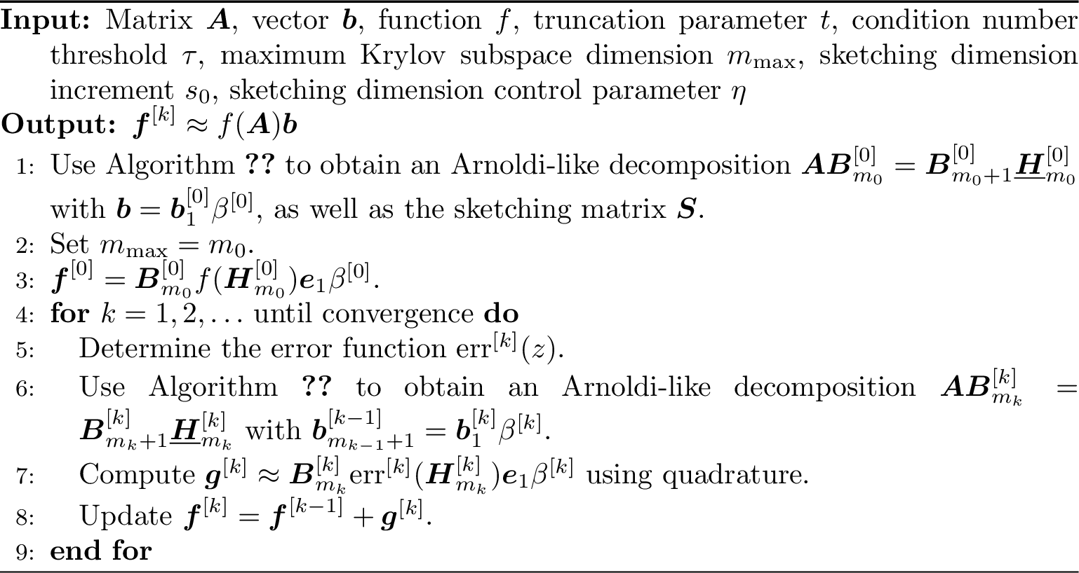
Using \(\boldsymbol{b}_{m + 1}\) as the new starting vector, suppose that a new Arnoldi-like decomposition \(\boldsymbol{A}\boldsymbol{B}_{m}^{+} = \boldsymbol{B}_{m + 1}^{+}\underline{\boldsymbol{H}}_{m}^{+}\) is generated with \(\boldsymbol{b}_{m + 1} = \boldsymbol{b}_{1}^{+}\beta^{+}\). Then the error term can itself be approximated by an Arnoldi-like approximation: \[\mathrm{err}(\boldsymbol{A})\boldsymbol{b}_{m + 1} = \boldsymbol{B}_{m}^{+}\mathrm{err}(\boldsymbol{H}_{m}^{+})\boldsymbol{e}_{1}\beta^{+} + \mathrm{err}^{+}(\boldsymbol{A})\boldsymbol{b}_{m + 1}^{+},\] where \(\mathrm{err}^{+}(z)\) is the new error function. Repeating this process yields the general restarting framework in Algorithm 1. The corresponding error functions \(\mathrm{err}^{[k]}(z)\) are given in Corollary 1. Although the corollary assumes a fixed Krylov subspace dimension \(m\) in each restart cycle, the result extends directly to variable dimensions.
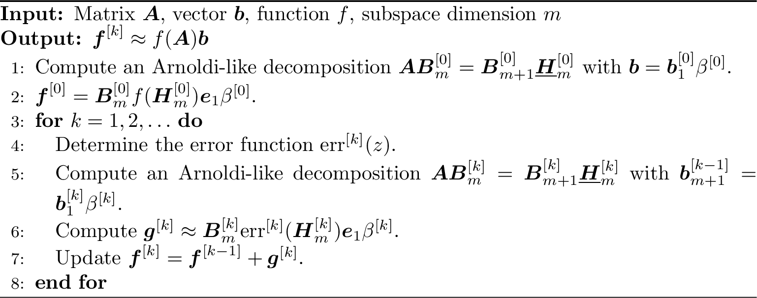
Corollary 1 (Error of the Arnoldi-like approximation after \(k\) restarts). Under the assumptions of Theorem 1, suppose that the \(\ell\)-th cycle generates an Arnoldi-like decomposition \(\boldsymbol{A}\boldsymbol{B}_{m}^{[\ell]} = \boldsymbol{B}_{m + 1}^{[\ell]}\underline{\boldsymbol{H}}_{m}^{[\ell]}\) for \(0 \leq \ell \leq k\). Here, \(\boldsymbol{b} = \boldsymbol{b}_{1}^{[0]}\beta^{[0]}\) and \(\boldsymbol{b}_{m + 1}^{[\ell - 1]} = \boldsymbol{b}_{1}^{[\ell]}\beta^{[\ell]}\) for \(1 \leq \ell \leq k\). Assume that \(\varLambda(\boldsymbol{H}_{m}^{[\ell]}) = \{\theta_{j}^{[\ell]}\}_{j = 1}^{m} \subset \Omega\), and define \(\phi_{m}^{[\ell]}(t) = \prod_{j = 1}^{m}(t - \theta_{j}^{[\ell]})\) and \(\gamma_{m}^{[\ell]} = \prod_{j = 1}^{m}h_{j + 1, j}^{[\ell]}\) for \(0 \leq \ell \leq k\). Then the error after \(k\) restarts is \[\begin{align} f(\boldsymbol{A})\boldsymbol{b} - \boldsymbol{f}^{[k]} &= \biggl( \prod_{\ell = 0}^{k}\gamma_{m}^{[\ell]}\beta^{[\ell]} \biggr) \biggl( \int_{\Gamma} \frac{g(t)}{\prod_{\ell = 0}^{k}\phi_{m}^{[\ell]}(t)} (t\boldsymbol{I} - \boldsymbol{A})^{-1} \,\mathrm{d}t \biggr) \boldsymbol{b}_{m + 1}^{[k]} \\ &\eqcolon \mathrm{err}^{[k + 1]}(\boldsymbol{A})\boldsymbol{b}_{m + 1}^{[k]}. \end{align}\]
In practice, the error functions are evaluated using adaptive quadrature. For a given error function, we compute two quadrature approximations using \(r_{1}\) and \(r_{2}\) nodes, where \(r_{2} = 2r_{1}\). The approximation based on \(r_{2}\) nodes is accepted if the corresponding reduced vectors differ by less than a prescribed tolerance. Otherwise, we set \(r_{1} = r_{2}\), double \(r_{2}\), and repeat the test until the tolerance is satisfied or a prescribed maximum number of nodes is reached. If no increase in the number of quadrature nodes is required in a given iteration, we reduce the quadrature sizes for the next iteration by setting \(r_{2} = r_{1}\) and halving \(r_{1}\).
3.2 Restarting Krylov and sketched Krylov subspace methods↩︎
The discussion above links the Arnoldi-like framework of Section 2 with the quadrature-based restarting mechanism. Indeed, the Arnoldi approximation 6 , the HmArnoldi approximation 8 , the sArnoldi approximation 12 , and the sHmArnoldi approximation 14 are all special cases of the Arnoldi-like approximation 15 , provided that the corresponding orthogonality conditions are satisfied. Thus, the same error representation and restarting mechanism apply to all these approximations. This observation forms the basis of the sketch-and-restart framework developed in the next section. Different basis generation processes lead to different restarted algorithms, while the underlying restarting formula remains unchanged.
4 Sketch-and-restart algorithms for matrix functions↩︎
The previous section showed that quadrature-based restarting applies to any Arnoldi-like approximation of the form \(\boldsymbol{B}_{m}f(\boldsymbol{H}_{m})\boldsymbol{e}_{1}\beta\), provided that the required orthogonality condition is satisfied. In this section, we instantiate this restarting mechanism using different strategies for generating Arnoldi-like decompositions. Specifically, we consider three such strategies: the existing sketched Arnoldi process, a new sketched harmonic Arnoldi process introduced in this work, and an adaptive truncated Arnoldi process combined with a rank-\(1\) update. These strategies lead to two restarted algorithms for computing \(f(\boldsymbol{A})\boldsymbol{b}\).
4.1 Basis generation↩︎
The standard Arnoldi process [13] generates an orthonormal basis for the Krylov subspace \(\mathcal{K}_{m}(\boldsymbol{A}, \boldsymbol{b})\), but its orthogonalization and storage costs can become substantial when \(m\) is large. In the sketch-and-restart framework, full orthogonality is not required. It suffices to construct an Arnoldi-like decomposition that satisfies the orthogonality condition required by the corresponding approximation. We therefore consider three basis generation strategies that produce possibly nonorthonormal bases with different computational and storage trade-offs.
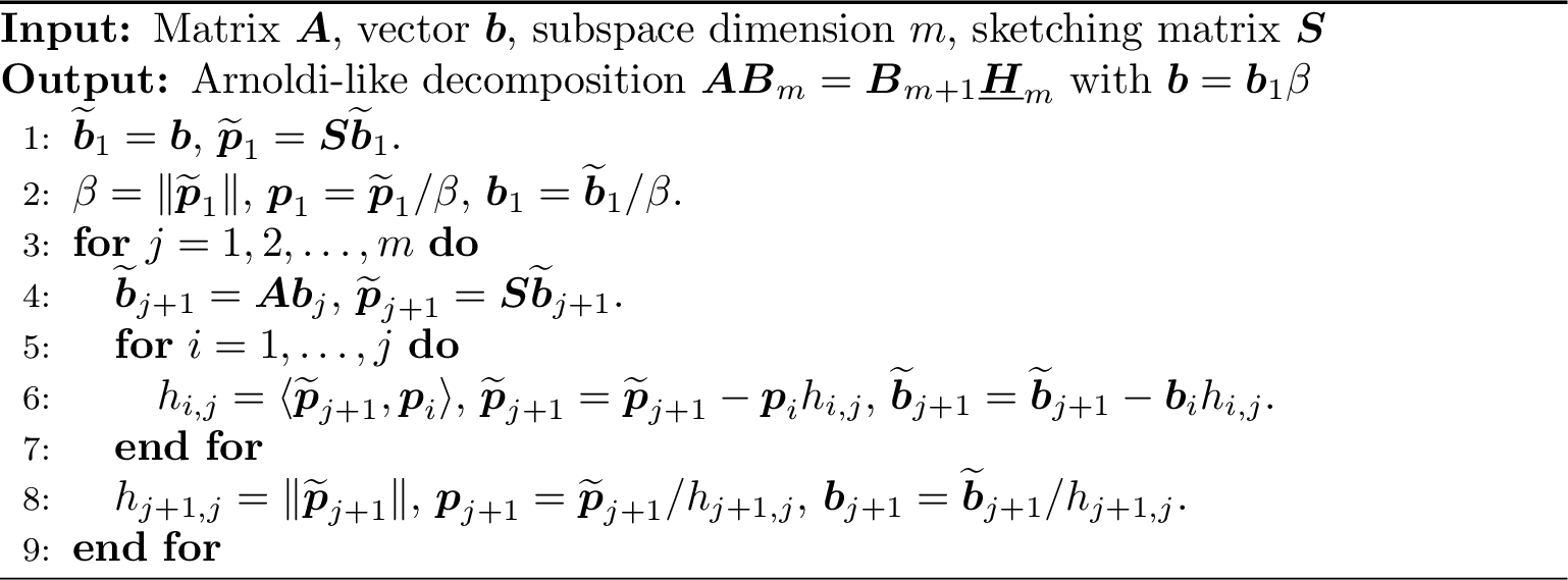
The first strategy is the sketched Arnoldi (s-Arnoldi) process [10], [18]. It is based on the Arnoldi process but computes the Gram–Schmidt coefficients in the sketched space. The same coefficients are then used to update the full-space basis vectors, as summarized in Algorithm 2. For simplicity, we assume that no breakdown occurs. The process yields a standard Arnoldi decomposition in the sketched space. Consequently, the resulting Arnoldi-like decomposition satisfies \(\boldsymbol{b}_{m + 1} \perp_{\boldsymbol{S}} \boldsymbol{B}_{m}\), and the sArnoldi approximation can be computed directly from 12 . The complexity of the s-Arnoldi process is \(\mathscr{O}(m T_{\mathrm{apply}} + m T_{\mathrm{sketching}} + N m^{2} + m^{3})\), where \(T_{\mathrm{apply}}\) and \(T_{\mathrm{sketching}}\) denote the costs of applying \(\boldsymbol{A}\) and \(\boldsymbol{S}\) to a vector, respectively. Compared with the standard Arnoldi process, s-Arnoldi reduces the orthogonalization cost by nearly one half, while the additional costs are of lower order.
The second strategy is the sketched harmonic Arnoldi (sHm-Arnoldi) process, which, to the best of our knowledge, is new. It is similar to the s-Arnoldi process but aims to generate a nonorthonormal basis such that \(\boldsymbol{b}_{j + 1} \perp_{\boldsymbol{S}} \boldsymbol{A}\boldsymbol{B}_{j}\) for \(1 \leq j \leq m\). In particular, the resulting Arnoldi-like decomposition satisfies \(\boldsymbol{b}_{m + 1} \perp_{\boldsymbol{S}} \boldsymbol{A}\boldsymbol{B}_{m}\), so the sHmArnoldi approximation can be computed directly from 14 . The procedure, summarized in Algorithm 3, orthogonalizes each new sketched basis vector against the sketched images of the current basis vectors under \(\boldsymbol{A}\), thereby enforcing \(\langle \boldsymbol{p}_{j + 1},\boldsymbol{z}_{i}\rangle = 0\) for \(1 \leq i \leq j\), where \(\boldsymbol{z}_{i} = \boldsymbol{q}_{i}/\rho_{i}^{*}\) is scaled so that \(\langle \boldsymbol{p}_{i},\boldsymbol{z}_{i}\rangle = 1\). The complexity of sHm-Arnoldi is \(\mathscr{O}(m T_{\mathrm{apply}} + m T_{\mathrm{sketching}} + N m^{2} + m^{3})\), and its orthogonalization cost is nearly one half of that of the standard Arnoldi process.

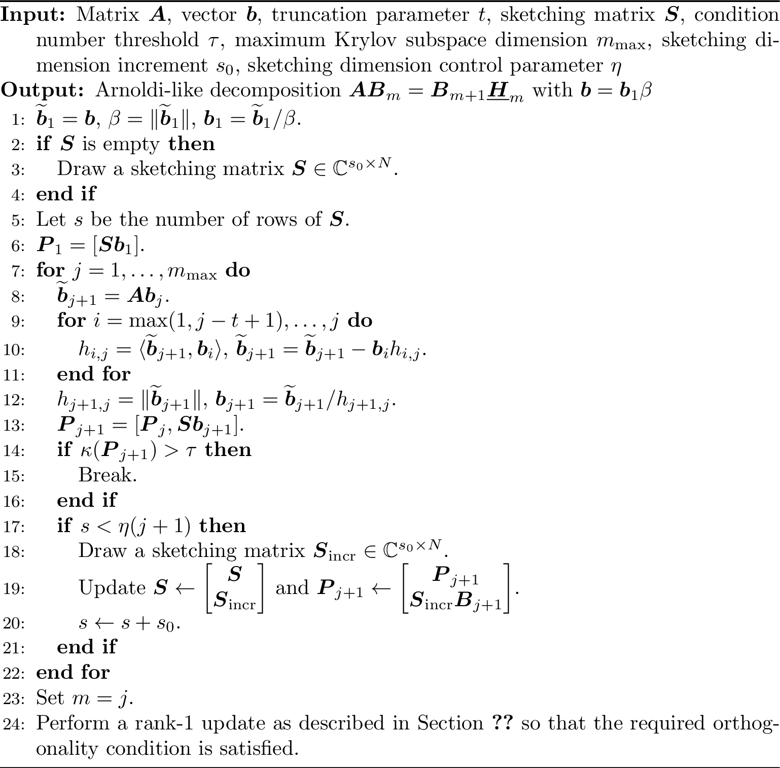
The third strategy is the truncated Arnoldi (\(t\)-Arnoldi) process [13]. It generates a nonorthonormal basis by orthogonalizing each new vector only against the \(t\) most recently generated basis vectors. We use this process adaptively by monitoring the condition number of the sketched basis \(\boldsymbol{S}\boldsymbol{B}_{m}\). Once this condition number exceeds a prescribed threshold \(\tau\), the process is terminated, and a rank-\(1\) update is applied to enforce the required orthogonality condition, as discussed in Section 2.3. Since the resulting Krylov subspace dimension is typically small, the rank-\(1\) update is inexpensive and can be performed at the BLAS-2 level. The complete procedure is summarized in Algorithm 4 and has complexity \(\mathscr{O}(m T_{\mathrm{apply}} + m T_{\mathrm{sketching}} + N m^{2})\).
4.2 Algorithms↩︎
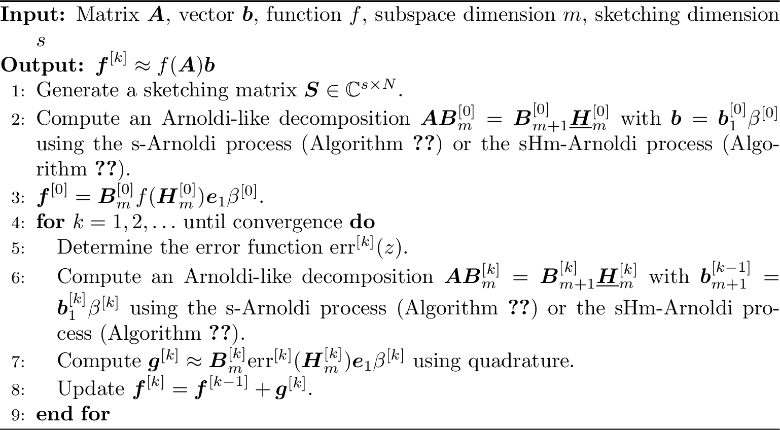
We now present two algorithmic realizations of the sketch-and-restart framework. Algorithm 5 uses a fixed Krylov subspace dimension and applies either the s-Arnoldi or the sHm-Arnoldi process in each restart cycle, leading respectively to the restarted sArnoldi and restarted sHmArnoldi methods. The error function is updated as in Algorithm 1, and the correction term is evaluated by quadrature. Algorithm 6 instead chooses the Krylov subspace dimension adaptively using the \(t\)-Arnoldi process. The dimension \(m_{0}\) obtained in the first restart cycle is used as the upper bound \(m_{\max}\) in all subsequent cycles. The same quadrature-based restarting mechanism is then applied to the resulting Arnoldi-like decompositions.
5 Convergence analysis↩︎
In this section, we analyze the convergence of the proposed sketch-and-restart algorithms. We assume exact arithmetic and neglect quadrature errors, so the analysis focuses on the Krylov and sketching components of the methods. The non-sketched adaptive variants can be related directly to existing restarted Arnoldi and harmonic Arnoldi methods through the Arnoldi-like framework developed above. The main new issue is the convergence of the restarted sketched harmonic Arnoldi method, for which the Petrov–Galerkin condition is imposed only after applying the sketching matrix.
Our analysis extends the GMRES-based approach of [19] to the sketched setting. This approach is particularly useful because it does not rely on CG-type arguments and therefore remains applicable in the presence of complex Ritz values. We focus on Stieltjes functions of the form \[\label{eq:stieltjes95func} f(z) = \int_{-\infty}^{0} \frac{g(t)}{t - z} \,\mathrm{d}t,\tag{16}\] where \(g\) is a suitable nonpositive function on \((-\infty, 0]\).
5.1 Harmonic Arnoldi approximation with a nonorthogonal basis↩︎
We first consider the non-sketched adaptive variants of Algorithm 6. We show that, after the rank-\(1\) update, these variants are mathematically equivalent to the restarted Arnoldi and HmArnoldi methods analyzed in [19], even though the basis generated by the \(t\)-Arnoldi process is not orthonormal.
Assume that we have an Arnoldi-like decomposition 4 , where \(\boldsymbol{B}_{m}\) has full column rank but is not necessarily orthonormal. We further assume that \(\boldsymbol{b}_{m + 1} \perp \boldsymbol{A}\boldsymbol{B}_{m}\), which can be enforced by the rank-\(1\) update discussed in Section 2.3. Under this assumption, Algorithm 6 is mathematically equivalent to the restarted HmArnoldi method analyzed in [19]. The corresponding HmArnoldi approximation to the solution of the shifted linear system 3 is \(\boldsymbol{x}_{m}(t) = \boldsymbol{B}_{m}(t\boldsymbol{I}_{m} - \boldsymbol{H}_{m})^{-1}\boldsymbol{e}_{1}\beta\). Its residual satisfies \[\begin{align} \boldsymbol{r}_{m}(t) &= \boldsymbol{b} - (t\boldsymbol{I} - \boldsymbol{A})\boldsymbol{x}_{m}(t) \\ &= \boldsymbol{b} - (t\boldsymbol{I} - \boldsymbol{A}) \boldsymbol{B}_{m} (t\boldsymbol{I}_{m} - \boldsymbol{H}_{m})^{-1} \boldsymbol{e}_{1}\beta \\ &= \boldsymbol{b} - [\boldsymbol{B}_{m} \;\boldsymbol{b}_{m + 1}] (t\underline{\boldsymbol{I}}_{m} - \underline{\boldsymbol{H}}_{m}) (t\boldsymbol{I}_{m} - \boldsymbol{H}_{m})^{-1} \boldsymbol{e}_{1}\beta \\ &= \boldsymbol{b}_{m + 1} h_{m + 1,m} \boldsymbol{e}_{m}^{\top} (t\boldsymbol{I}_{m} - \boldsymbol{H}_{m})^{-1} \boldsymbol{e}_{1}\beta \\ &\eqcolon \boldsymbol{b}_{m + 1}\zeta(t). \end{align}\] Thus, the residual is collinear with \(\boldsymbol{b}_{m + 1}\) for all \(t\).
For each \(t\), let \(p_{m - 1,t} \in \mathcal{P}_{m - 1}\) be the polynomial that interpolates \(h_{t}(z) = (t - z)^{-1}\) at the harmonic Ritz values \(\varLambda(\boldsymbol{H}_{m})\). Then Lemma 2 gives \[\boldsymbol{x}_{m}(t) = \boldsymbol{B}_{m}(t\boldsymbol{I}_{m} - \boldsymbol{H}_{m})^{-1}\boldsymbol{e}_{1}\beta = p_{m - 1,t}(\boldsymbol{A})\boldsymbol{b}.\] If \(f\) is a Stieltjes function of the form 16 , then the HmArnoldi approximation 8 can be written as \(\boldsymbol{f}_{m} = \int_{-\infty}^{0} g(t)\boldsymbol{x}_{m}(t) \,\mathrm{d}t\). Up to the sign convention in the Stieltjes representation, this is precisely the class of HmArnoldi approximants analyzed in [19]. Consequently, the convergence results of [19] carry over to Algorithm 6. The following theorem summarizes this observation.
Theorem 2 (Convergence of the adaptive restarted Arnoldi-like method). Let \(f\) be a Stieltjes function, and consider Algorithm 6, where the basis is generated by the truncated Arnoldi process in Algorithm 4.
If the rank-\(1\) update enforces \(\boldsymbol{b}_{m + 1} \perp \boldsymbol{B}_{m}\), then the algorithm is mathematically equivalent to the restarted Arnoldi method for computing \(f(\boldsymbol{A})\boldsymbol{b}\). Hence, if \(\boldsymbol{A}\) is Hermitian positive definite, the method converges for every restart length \(m \geq 1\).
If the rank-\(1\) update enforces \(\boldsymbol{b}_{m + 1} \perp \boldsymbol{A}\boldsymbol{B}_{m}\), then the algorithm is mathematically equivalent to the restarted HmArnoldi method for computing \(f(\boldsymbol{A})\boldsymbol{b}\). Hence, if \(\boldsymbol{A}\) is positive real, the method converges for every restart length \(m \geq 1\).
Proof. The equivalence to the restarted Arnoldi and restarted HmArnoldi methods follows from the Arnoldi-like framework and the rank-\(1\) update described above. The convergence of the restarted Arnoldi method for Hermitian positive definite matrices is established in [19], while the convergence of the restarted HmArnoldi method for positive real matrices is proved in [19]. Since both convergence results hold for every restart length \(m \geq 1\), they remain valid when the restart length varies between restart cycles. ◻
5.2 Sketched harmonic Arnoldi with a nonorthogonal basis↩︎
We now turn to the sketched setting, where the Petrov–Galerkin condition is imposed only after applying the sketching matrix. Unlike the non-sketched variants discussed above, the restarted sHmArnoldi method cannot be reduced directly to the HmArnoldi method analyzed in [19]. We therefore establish the residual relations needed to extend the GMRES-based convergence analysis to the sketched setting.
Suppose that, in the Arnoldi-like decomposition 4 , the matrix \(\boldsymbol{B}_{m}\) has full column rank but is not necessarily orthonormal. Assume further that \(\boldsymbol{b}_{m + 1} \perp_{\boldsymbol{S}} \boldsymbol{A}\boldsymbol{B}_{m}\). The sHmArnoldi approximation to the solution of the shifted linear system 3 is \(\widehat{\boldsymbol{x}}_{m}(t) = \boldsymbol{B}_{m}(t\boldsymbol{I}_{m} - \boldsymbol{H}_{m})^{-1}\boldsymbol{e}_{1}\beta\). As in Section 5.1, its residual satisfies \[\label{eq:s95hm95arnoldi95res} \widehat{\boldsymbol{r}}_{m}(t) = \boldsymbol{b} - (t\boldsymbol{I} - \boldsymbol{A})\widehat{\boldsymbol{x}}_{m}(t) = \boldsymbol{b}_{m + 1}\widehat{\zeta}(t).\tag{17}\] Thus, the residual is collinear with \(\boldsymbol{b}_{m + 1}\) for all \(t\).
Similarly, for each \(t\), there exists a polynomial \(\widehat{p}_{m - 1,t} \in \mathcal{P}_{m - 1}\) such that \(\widehat{\boldsymbol{x}}_{m}(t) = \widehat{p}_{m - 1,t}(\boldsymbol{A})\boldsymbol{b}\), where \(\widehat{p}_{m - 1,t}\) interpolates \(h_{t}(z) = (t - z)^{-1}\) at the sketched harmonic Ritz values \(\varLambda(\boldsymbol{H}_{m})\). Therefore, the residual can be written as \[\widehat{\boldsymbol{r}}_{m}(t) = \widehat{q}_{m,t}(\boldsymbol{A})\boldsymbol{b}, \qquad \widehat{q}_{m,t}(z) = 1 - (t - z)\widehat{p}_{m - 1,t}(z).\] The following lemma is the sketched analogue of [19]. We include a direct proof for completeness.
Lemma 3 (A formula for the residual). Let \(\varLambda(\boldsymbol{H}_{m}) = \{\theta_{1}, \dotsc, \theta_{m}\}\), and assume that \(\theta_{j} \neq 0\) for \(j = 1, \dotsc, m\). Then the residuals defined in 17 satisfy \[\widehat{\boldsymbol{r}}_{m}(t) = \frac{1}{(1 - t/\theta_{1})\dotsm(1 - t/\theta_{m})} \widehat{\boldsymbol{r}}_{m}(0) \eqcolon \widehat{\boldsymbol{r}}_{m}(0)\eta_{m}(t).\]
Proof. Let \(\phi_{m}(z) = (z - \theta_{1})\dotsm(z - \theta_{m})\). It is straightforward to verify that \(\widehat{p}_{m - 1,t}(z) = \bigl(1 - \phi_{m}(z)/\phi_{m}(t)\bigr)/(t - z)\) is the polynomial interpolating \(h_{t}(z) = (t - z)^{-1}\) at \(\varLambda(\boldsymbol{H}_{m})\). Direct substitution gives \(\widehat{q}_{m,t}(z) = 1 - (t - z)\widehat{p}_{m - 1,t}(z) = \phi_{m}(z)/\phi_{m}(t)\). Therefore, \[\widehat{\boldsymbol{r}}_{m}(t) = \widehat{q}_{m,t}(\boldsymbol{A})\boldsymbol{b} = \frac{\phi_{m}(\boldsymbol{A})}{\phi_{m}(t)}\boldsymbol{b} = \frac{\phi_{m}(0)}{\phi_{m}(t)} \frac{\phi_{m}(\boldsymbol{A})}{\phi_{m}(0)} \boldsymbol{b} = \frac{\phi_{m}(0)}{\phi_{m}(t)} \widehat{\boldsymbol{r}}_{m}(0).\] Since \(\phi_{m}(t)/\phi_{m}(0) = (1 - t/\theta_{1})\dotsm(1 - t/\theta_{m})\), the stated formula follows. ◻
Suppose that \(\boldsymbol{A}\) is positive real. If the sketched harmonic Ritz values \(\varLambda(\boldsymbol{H}_{m})\) lie in the open right half-plane \(\mathbb{C}_{+}\), the modulus of the factor \(\phi_{m}(0)/\phi_{m}(t)\) decreases as \(t\) moves from \(0\) toward \(-\infty\). Moreover, \(\widehat{\boldsymbol{r}}_{m}(0)\) is precisely the residual of the sGMRES approximant \(\widehat{\boldsymbol{x}}_{m}(0)\). The following lemma provides a bound for \(\|\widehat{\boldsymbol{r}}_{m}(0)\|\).
Lemma 4 (Bound on the residual). Let \(\boldsymbol{A} \in \mathbb{C}^{N \times N}\) be positive real, and let \(\boldsymbol{b} \in \mathbb{C}^{N}\). Let \(\widehat{\boldsymbol{x}}_{m}(t)\) be the sHmArnoldi approximation to the solution of the shifted linear system 3 , and let \(\widehat{\boldsymbol{r}}_{m}(t)\) be the corresponding residual defined in 17 . Then \[\|\widehat{\boldsymbol{r}}_{m}(0)\| \leq C_{\varepsilon}\alpha_{m}\|\boldsymbol{b}\|,\] where \(C_{\varepsilon} = \sqrt{(1 + \varepsilon)/(1 - \varepsilon)}\) and \(\alpha_{m} = (1 - \delta\delta^{\prime})^{m/2} \in [0,1)\). The constants \(\delta\) and \(\delta^{\prime}\) are defined by \[\label{eq:delta95delta95prime} \begin{align} \delta &= \min \bigl\{ |\boldsymbol{v}^{*}\boldsymbol{A}\boldsymbol{v}| : \boldsymbol{v} \in \mathbb{C}^{N}, \;\|\boldsymbol{v}\| = 1 \bigr\}, \\ \delta^{\prime} &= \min \bigl\{ |\boldsymbol{v}^{*}\boldsymbol{A}^{-1}\boldsymbol{v}| : \boldsymbol{v} \in \mathbb{C}^{N}, \;\|\boldsymbol{v}\| = 1 \bigr\}. \end{align}\qquad{(3)}\]
Proof. Let \(\boldsymbol{x}_{m}(t)\) be the HmArnoldi approximation to the solution of the shifted linear system 3 , and let \(\boldsymbol{r}_{m}(t)\) be the corresponding residual. By [19], \(\|\boldsymbol{r}_{m}(0)\| \leq \alpha_{m}\|\boldsymbol{b}\|\). Since the subspace embedding property holds for the relevant residual vectors, by the sketched residual minimization property of sGMRES, we have \[\|\widehat{\boldsymbol{r}}_{m}(0)\| \leq \frac{1}{\sqrt{1 - \varepsilon}} \|\boldsymbol{S}\widehat{\boldsymbol{r}}_{m}(0)\| \leq \frac{1}{\sqrt{1 - \varepsilon}} \|\boldsymbol{S}\boldsymbol{r}_{m}(0)\| \leq \sqrt{\frac{1 + \varepsilon}{1 - \varepsilon}} \|\boldsymbol{r}_{m}(0)\|.\] Combining the above estimate with \(\|\boldsymbol{r}_{m}(0)\| \leq \alpha_{m}\|\boldsymbol{b}\|\) completes the proof. ◻
For a Stieltjes function \(f\) of the form 16 , the sHmArnoldi approximation to \(f(\boldsymbol{A})\boldsymbol{b}\) can be written as \(\widehat{\boldsymbol{f}}_{m} = \int_{-\infty}^{0} g(t)\widehat{\boldsymbol{x}}_{m}(t) \,\mathrm{d}t\). Consequently, \[\begin{align} f(\boldsymbol{A})\boldsymbol{b} - \widehat{\boldsymbol{f}}_{m} &= \int_{-\infty}^{0} g(t) \bigl( \boldsymbol{x}(t) - \widehat{\boldsymbol{x}}_{m}(t) \bigr) \,\mathrm{d}t \\ &= \int_{-\infty}^{0} g(t) (t\boldsymbol{I} - \boldsymbol{A})^{-1} \bigl( \boldsymbol{b} - (t\boldsymbol{I} - \boldsymbol{A})\widehat{\boldsymbol{x}}_{m}(t) \bigr) \,\mathrm{d}t \\ &= \int_{-\infty}^{0} g(t) (t\boldsymbol{I} - \boldsymbol{A})^{-1} \widehat{\boldsymbol{r}}_{m}(t) \,\mathrm{d}t \\ &= \int_{-\infty}^{0} g(t) (t\boldsymbol{I} - \boldsymbol{A})^{-1} \eta_{m}(t)\widehat{\boldsymbol{r}}_{m}(0) \,\mathrm{d}t \\ &= \mathrm{err}(\boldsymbol{A})\widehat{\boldsymbol{r}}_{m}(0), \end{align}\] where \(\mathrm{err}(z) = \int_{-\infty}^{0} g(t)\eta_{m}(t)(t - z)^{-1} \,\mathrm{d}t\). Combining the above discussion, we obtain the convergence of the restarted sHmArnoldi method for computing \(f(\boldsymbol{A})\boldsymbol{b}\) when \(\boldsymbol{A}\) is positive real and \(f\) is a Stieltjes function.
Theorem 3 (Convergence of the restarted sHmArnoldi method). Let \(\boldsymbol{A} \in \mathbb{C}^{N \times N}\) be positive real, let \(\boldsymbol{b} \in \mathbb{C}^{N}\), and let \(f\) be a Stieltjes function of the form 16 . Assume that the sketched harmonic Ritz values satisfy \(\theta_{j}^{[\ell]} \in \mathbb{C}_{+}\) for \(0 \leq \ell \leq k\) and \(1 \leq j \leq m\). Then the restarted sHmArnoldi approximation computed by Algorithm 5 satisfies \[\label{eq:sketched95harmonic95bound} \bigl\| f(\boldsymbol{A})\boldsymbol{b} - \widehat{\boldsymbol{f}}^{[k]} \bigr\|_{\boldsymbol{A}^{*}\boldsymbol{A}} \leq C\|\boldsymbol{b}\| \bigl(C_{\varepsilon}\alpha_{m}\bigr)^{k + 1},\qquad{(4)}\] where \(C = \sqrt{\nu_{\max}}f(\rho\nu_{\max})\), and \(\alpha_{m}\) and \(C_{\varepsilon}\) are defined in Lemma 4. Here, \[\label{eq:nu95max95rho} \begin{align} \nu_{\max} &= \max \bigl\{ \boldsymbol{v}^{*}\boldsymbol{A}^{*}\boldsymbol{A}\boldsymbol{v} : \boldsymbol{v} \in \mathbb{C}^{N}, \;\|\boldsymbol{v}\| = 1 \bigr\} = \|\boldsymbol{A}\|^{2}, \\ \rho &= \min \bigl\{ \Re\bigl( \boldsymbol{v}^{*}\boldsymbol{A}^{-1}\boldsymbol{v} \bigr) : \boldsymbol{v} \in \mathbb{C}^{N}, \;\|\boldsymbol{v}\| = 1 \bigr\}. \end{align}\qquad{(5)}\] Since \(\boldsymbol{A}\) is positive real, we have \(\rho > 0\). Thus, \(\rho\nu_{\max} > 0\), and the representation 16 with \(g\) nonpositive implies that \(f(\rho\nu_{\max}) > 0\).
Proof. By Lemma 3, the residual in the \(\ell\)-th cycle satisfies \(\widehat{\boldsymbol{r}}_{m}^{[\ell]}(t) = \widehat{\boldsymbol{r}}_{m}^{[\ell]}(0)\eta_{m}^{[\ell]}(t)\). Following the argument in Corollary 1, the remaining error after \(k\) restart cycles can be written as \[f(\boldsymbol{A})\boldsymbol{b} - \widehat{\boldsymbol{f}}^{[k]} = \biggl( \int_{-\infty}^{0} g(t) \prod_{\ell = 0}^{k}\eta_{m}^{[\ell]}(t) (t\boldsymbol{I} - \boldsymbol{A})^{-1} \,\mathrm{d}t \biggr) \widehat{\boldsymbol{r}}_{m}^{[k]}(0).\] Since \(\Re(\theta_{j}^{[\ell]}) > 0\), we have \(\Re(-t/\theta_{j}^{[\ell]}) \geq 0\) for all \(t \leq 0\). Hence, \(|1 - t/\theta_{j}^{[\ell]}| \geq 1\), and \[|\eta_{m}^{[\ell]}(t)| = \prod_{j = 1}^{m} \frac{1}{|1 - t/\theta_{j}^{[\ell]}|} \leq 1, \qquad 0 \leq \ell \leq k, \quad t \leq 0.\] Following the proof of [19] and using \(|\eta_{m}^{[\ell]}(t)| \leq 1\), we obtain \[\bigl\| f(\boldsymbol{A})\boldsymbol{b} - \widehat{\boldsymbol{f}}^{[k]} \bigr\|_{\boldsymbol{A}^{*}\boldsymbol{A}} \leq \|\widehat{\boldsymbol{r}}_{m}^{[k]}(0)\| \int_{-\infty}^{0} g(t) \frac{\sqrt{\nu_{\max}}}{t - \rho\nu_{\max}} \,\mathrm{d}t = \|\widehat{\boldsymbol{r}}_{m}^{[k]}(0)\| \sqrt{\nu_{\max}} f(\rho\nu_{\max}).\] Here, we used the fact that \(g\) is nonpositive in the Stieltjes representation 16 . Finally, Lemma 4 gives \(\|\widehat{\boldsymbol{r}}_{m}^{[k]}(0)\| \leq C_{\varepsilon}\alpha_{m} \|\widehat{\boldsymbol{r}}_{m}^{[k - 1]}(0)\|\). Applying this inequality recursively and defining \(C = \sqrt{\nu_{\max}}f(\rho\nu_{\max})\) completes the proof. ◻
Theorem 3 states that, if the sketching matrix \(\boldsymbol{S}\) provides a sufficiently accurate embedding for the subspace spanned by \(\boldsymbol{B}_{m + 1}\) in each restart cycle, then the restarted sHmArnoldi method converges geometrically. More precisely, this requires \(C_{\varepsilon}\alpha_{m} < 1\) and the sketched harmonic Ritz values to satisfy \(\theta_{j}^{[\ell]} \in \mathbb{C}_{+}\). Both conditions can be satisfied when the embedding distortion \(\varepsilon\) is sufficiently small. While \(C_{\varepsilon}\) depends explicitly on \(\varepsilon\), the location of the sketched harmonic Ritz values is less transparent and also depends on the sketching matrix \(\boldsymbol{S}\). The following subsection investigates this issue.
5.3 Sketched harmonic Ritz values↩︎
The convergence result in Theorem 3 assumes that all sketched harmonic Ritz values lie in the open right half-plane. This subsection provides a sufficient condition under which this assumption holds. The argument relies only on the orthogonality condition produced by the sHm-Arnoldi process, namely, \(\boldsymbol{b}_{m + 1} \perp_{\boldsymbol{S}} \boldsymbol{A}\boldsymbol{B}_{m}\).
Denote \(\boldsymbol{W}_{m} = \boldsymbol{A}\boldsymbol{B}_{m}\). Since \(\boldsymbol{b}_{m + 1} \perp_{\boldsymbol{S}} \boldsymbol{A}\boldsymbol{B}_{m}\), multiplying the Arnoldi-like decomposition 4 from the left by \((\boldsymbol{S}\boldsymbol{W}_{m})^{*}\boldsymbol{S}\) gives \[(\boldsymbol{S}\boldsymbol{W}_{m})^{*} (\boldsymbol{S}\boldsymbol{W}_{m}) = (\boldsymbol{S}\boldsymbol{W}_{m})^{*} (\boldsymbol{S}\boldsymbol{B}_{m}) \boldsymbol{H}_{m}.\] Therefore, \(\boldsymbol{H}_{m} = \boldsymbol{G}_{m}^{-1}\boldsymbol{F}_{m}\), where \(\boldsymbol{G}_{m} = (\boldsymbol{S}\boldsymbol{W}_{m})^{*}(\boldsymbol{S}\boldsymbol{B}_{m})\) and \(\boldsymbol{F}_{m} = (\boldsymbol{S}\boldsymbol{W}_{m})^{*}(\boldsymbol{S}\boldsymbol{W}_{m})\), provided that \(\boldsymbol{G}_{m}\) is nonsingular. Thus, the sketched harmonic Ritz values are the generalized eigenvalues of the matrix pencil \((\boldsymbol{F}_{m},\boldsymbol{G}_{m})\).
Let \(\theta \in \varLambda(\boldsymbol{H}_{m})\), and let \(\boldsymbol{y} \in \mathbb{C}^{m}\) be a corresponding nonzero eigenvector. Set \(\boldsymbol{x} = \boldsymbol{W}_{m}\boldsymbol{y}\). Then \(\boldsymbol{x} \neq \boldsymbol{0}\) and \(\boldsymbol{F}_{m}\boldsymbol{y} = \boldsymbol{G}_{m}\boldsymbol{y}\theta\). This gives \[\theta = \frac{\boldsymbol{y}^{*}\boldsymbol{F}_{m}\boldsymbol{y}}{\boldsymbol{y}^{*}\boldsymbol{G}_{m}\boldsymbol{y}} = \frac{\|\boldsymbol{S}\boldsymbol{x}\|^{2}}{(\boldsymbol{S}\boldsymbol{x})^{*} (\boldsymbol{S}\boldsymbol{A}^{-1}\boldsymbol{x})}.\] Equivalently, \[\label{eq:recip95s95hm95ritz95value} \frac{1}{\theta} = \frac{(\boldsymbol{S}\boldsymbol{x})^{*} (\boldsymbol{S}\boldsymbol{A}^{-1}\boldsymbol{x})}{\|\boldsymbol{S}\boldsymbol{x}\|^{2}}.\tag{18}\]
Taking \(\boldsymbol{u} = \boldsymbol{A}^{-1}\boldsymbol{x} = \boldsymbol{B}_{m}\boldsymbol{y}\) and \(\boldsymbol{v} = \boldsymbol{x} = \boldsymbol{A}\boldsymbol{B}_{m}\boldsymbol{y}\) in the inner-product form of the subspace embedding property 10 , we obtain \[\bigl| (\boldsymbol{S}\boldsymbol{x})^{*} (\boldsymbol{S}\boldsymbol{A}^{-1}\boldsymbol{x}) - \boldsymbol{x}^{*}\boldsymbol{A}^{-1}\boldsymbol{x} \bigr| \leq \varepsilon \|\boldsymbol{A}^{-1}\boldsymbol{x}\| \|\boldsymbol{x}\| \leq \varepsilon \|\boldsymbol{A}^{-1}\| \|\boldsymbol{x}\|^{2}.\] Combining this estimate with the subspace embedding property 9 and the identity 18 , we conclude that the reciprocal of every sketched harmonic Ritz value satisfies \[\frac{1}{\theta} \in \biggl\{ \frac{z_{1} + z_{2}}{\tau} : z_{1} \in \mathcal{W}(\boldsymbol{A}^{-1}),\; |z_{2}| \leq \varepsilon\|\boldsymbol{A}^{-1}\|,\; 1 - \varepsilon \leq \tau \leq 1 + \varepsilon \biggr\}.\]
Since \(\boldsymbol{A}\) is positive real, \(\boldsymbol{A}^{-1}\) is also positive real. Let \(\rho\) be defined as in ?? . If \(\varepsilon\|\boldsymbol{A}^{-1}\| < \rho\), then, for any sketched harmonic Ritz value \(\theta\), the preceding inclusion gives \[\Re\biggl(\frac{1}{\theta}\biggr) \geq \frac{\rho - \varepsilon\|\boldsymbol{A}^{-1}\|}{1 + \varepsilon} > 0.\] Since \(\Re(1/\theta) > 0\) is equivalent to \(\Re(\theta) > 0\), all sketched harmonic Ritz values lie in the open right half-plane. Moreover, under the condition \(\varepsilon\|\boldsymbol{A}^{-1}\| < \rho\), for every nonzero \(\boldsymbol{y} \in \mathbb{C}^{m}\), with \(\boldsymbol{x} = \boldsymbol{A}\boldsymbol{B}_{m}\boldsymbol{y}\), we have \[\Re\bigl(\boldsymbol{y}^{*}\boldsymbol{G}_{m}\boldsymbol{y}\bigr) = \Re\bigl((\boldsymbol{S}\boldsymbol{x})^{*} (\boldsymbol{S}\boldsymbol{A}^{-1}\boldsymbol{x})\bigr) \geq \bigl(\rho-\varepsilon\|\boldsymbol{A}^{-1}\|\bigr)\|\boldsymbol{x}\|^{2} > 0.\] Hence, \(\boldsymbol{G}_{m}\) is nonsingular, and the condition \(\varepsilon\|\boldsymbol{A}^{-1}\| < \rho\) is sufficient for the sketched harmonic Ritz values generated by the sHm-Arnoldi process to lie in \(\mathbb{C}_{+}\), as required in Theorem 3.
6 Numerical experiments↩︎
In this section, we present numerical experiments to demonstrate the stability and efficiency of the proposed sketch-and-restart algorithms. The experiments illustrate the computational savings achieved through sketching, the storage reduction obtained by the adaptive \(t\)-Arnoldi process, and the effectiveness of thick restarting when aggressive truncation slows convergence. All algorithms are implemented in MATLAB R2023b, and all experiments are performed on a server equipped with two Intel Xeon Gold 6226R CPUs running at 2.90 GHz and 1000.6 GB of RAM. The code for reproducing the numerical experiments is available at https://github.com/JingyuLiuMath/funm_quad.
We use a sparse sign matrix [15] as the sketching matrix in all examples. Specifically, the matrix is defined as \[\boldsymbol{S} = \sqrt{\frac{1}{\zeta}} \begin{bmatrix} \boldsymbol{s}_{1} & \cdots & \boldsymbol{s}_{N} \end{bmatrix} \in \mathbb{C}^{s \times N},\] where \(\zeta\) is the sparsity parameter. Each vector \(\boldsymbol{s}_{i}\) is constructed by selecting \(\zeta\) entries uniformly at random and assigning them the values \(\pm 1\) with equal probability. Larger values of \(\zeta\) generally improve the embedding quality but increase the computational cost, whereas smaller values may lead to instability. Following the recommendation in [15], we set \(\zeta = \min\{s,8\}\). When the Krylov subspace dimension \(m\) is fixed, we set the sketching dimension to \(s = 2m\). Applying this sketching matrix to a vector therefore requires only \(\mathscr{O}(N)\) operations.
The quadrature tolerance and convergence tolerance are set to \(10^{-9}\) and \(10^{-7}\), respectively, and the maximum number of quadrature points is set to \(512\) in all examples. The relative error is computed using the exact solution. For Algorithm 5, we denote the variants based on the s-Arnoldi and sHm-Arnoldi processes by sArn and sHmArn, respectively. For comparison, we also use the quadrature-based restarted Arnoldi method of [4], which generates an orthonormal basis using the standard Arnoldi process and computes the Arnoldi approximation in each restart cycle. We denote this method by Arn.
For Algorithm 6, the initial maximum Krylov subspace dimension is set to \(m_{\max} = m\). In the \(t\)-Arnoldi process, we use \(t \in \{2,1,0\}\), the condition number threshold \(\tau = 10^{6}\), the sketching dimension increment \(s_{0} = 30\), and the sketching dimension control parameter \(\eta = 2\). At the end of each \(t\)-Arnoldi process, a rank-\(1\) update is applied to enforce either \(\boldsymbol{b}_{m + 1} \perp \boldsymbol{B}_{m}\) or \(\boldsymbol{b}_{m + 1} \perp \boldsymbol{A}\boldsymbol{B}_{m}\). We denote the corresponding methods by adaArn-\(t\) and adaHmArn-\(t\), respectively.
Finally, we use \(n_{\mathrm{iter}}\), \(n_{\mathrm{matvec}}\), and \(n_{\mathrm{vec}}\) to denote the number of restart cycles, the total number of matrix-vector products, and the maximum number of vectors stored simultaneously, respectively.
6.1 Convection-diffusion example↩︎
In this example, \(\boldsymbol{A}\) is obtained by discretizing a two-dimensional convection-diffusion operator on the unit square with a constant convection field in the direction \([1,-1]\) and diffusion coefficient \(D = 10^{-3}\). More precisely, \[\boldsymbol{A} = \frac{D}{h^{2}} \bigl( \boldsymbol{L} \otimes \boldsymbol{I} + \boldsymbol{I} \otimes \boldsymbol{L} \bigr) + \frac{1}{h} \bigl( \boldsymbol{C} \otimes \boldsymbol{I} + \boldsymbol{I} \otimes \boldsymbol{C}^{\top} \bigr) \in \mathbb{R}^{n^{2} \times n^{2}},\] where \(h = 1/(n + 1)\), \(\boldsymbol{L} \in \mathbb{R}^{n \times n}\) is the tridiagonal matrix with diagonal entries \(2\) and sub- and superdiagonal entries \(-1\), and \(\boldsymbol{C} \in \mathbb{R}^{n \times n}\) is the matrix with diagonal entries \(1\) and subdiagonal entries \(-1\). We choose \(n = 100\), so that \(N = 10{,}000\), and compute \(f(\boldsymbol{A})\boldsymbol{b}\) for \(f(z) = z^{-1/2}\), where \(\boldsymbol{b}\) is the vector of all ones normalized to unit norm. The Krylov subspace dimension is set to \(m = 150\).
| method | error | time (s) | \(n_{\iter}\) | \(n_{\matvec}\) | \(n_{\vecs}\) |
|---|---|---|---|---|---|
| Arn | 1.5e-08 | 1.7e+00 | 3 | 450 | 150 |
| sArn | 3.1e-09 | 1.2e+00 | 4 | 600 | 150 |
| sHmArn | 3.9e-09 | 1.2e+00 | 4 | 600 | 150 |
| adaArn-\(2\) | 1.5e-08 | 1.3e+00 | 3 | 450 | 150 |
| adaArn-\(1\) | 4.4e-08 | 8.3e-01 | 5 | 420 | 90 |
| adaArn-\(0\) | 2.8e-08 | 4.1e-01 | 19 | 263 | 15 |
| adaHmArn-\(2\) | 4.5e-08 | 1.2e+00 | 3 | 450 | 150 |
| adaHmArn-\(1\) | 1.4e-08 | 7.3e-01 | 4 | 355 | 90 |
| adaHmArn-\(0\) | 3.3e-08 | 4.1e-01 | 18 | 251 | 15 |

Table 1 and Figure 7 show that all methods attain the prescribed accuracy, with final relative errors of the same order of magnitude. Among the fixed-dimension methods, sArn and sHmArn require four restart cycles and \(600\) matrix-vector products, compared with three cycles and \(450\) matrix-vector products for Arn. Nevertheless, both sketched methods reduce the runtime from \(1.7\) seconds to \(1.2\) seconds. Thus, the lower cost of orthogonalization in the sketched space more than compensates for the additional restart cycle and matrix-vector products.
For both adaptive variants, decreasing the truncation parameter \(t\) substantially reduces the storage requirement, from \(150\) vectors for \(t = 2\) to \(90\) for \(t = 1\) and \(15\) for \(t = 0\). In this example, more aggressive truncation also reduces both the runtime and the total number of matrix-vector products. In particular, adaArn-0 and adaHmArn-0 require only \(263\) and \(251\) matrix-vector products, respectively, and both complete in \(0.41\) seconds while maintaining relative errors below the convergence tolerance. The results therefore indicate that, for this problem, aggressive truncation provides substantial savings in both storage and computational cost, despite increasing the number of restart cycles.
6.2 Lattice quantum chromodynamics example↩︎
This example arises from lattice quantum chromodynamics (QCD), where one needs to solve linear systems involving the overlap Dirac operator [20], \[\boldsymbol{N}_{\mathrm{ovl}} = \rho\boldsymbol{I} + \gamma_{5}\operatorname{sign}(\boldsymbol{Q}).\] Here, \(\rho > 1\), \(\gamma_{5}\) is a permutation matrix, and \(\boldsymbol{Q}\) is a large sparse matrix that becomes non-Hermitian in the presence of a nonzero chemical potential. Since forming \(\operatorname{sign}(\boldsymbol{Q})\) explicitly is infeasible, its action on a vector is computed as \[\operatorname{sign}(\boldsymbol{Q})\boldsymbol{b} = (\boldsymbol{Q}^{2})^{-1/2}\boldsymbol{Q}\boldsymbol{b}.\] In our experiment, \(N = 49{,}152\), \(\boldsymbol{b} = \boldsymbol{e}_{1}\), and \(m = 150\).
| method | error | time (s) | \(n_{\iter}\) | \(n_{\matvec}\) | \(n_{\vecs}\) |
|---|---|---|---|---|---|
| Arn | 4.7e-10 | 1.4e+01 | 3 | 450 | 150 |
| sArn | 1.3e-09 | 1.3e+01 | 3 | 450 | 150 |
| sHmArn | 1.6e-09 | 1.3e+01 | 3 | 450 | 150 |
| adaArn-\(2\) | 7.8e-09 | 1.2e+01 | 4 | 410 | 105 |
| adaArn-\(1\) | 9.9e-08 | 1.5e+01 | 40 | 722 | 20 |
| adaArn-\(0\) | 9.1e-08 | 1.9e+01 | 106 | 964 | 10 |
| adaHmArn-\(2\) | 1.2e-08 | 1.2e+01 | 4 | 415 | 105 |
| adaHmArn-\(1\) | 9.6e-08 | 1.6e+01 | 41 | 740 | 20 |
| adaHmArn-\(0\) | 9.8e-08 | 2.8e+01 | 142 | 1279 | 10 |
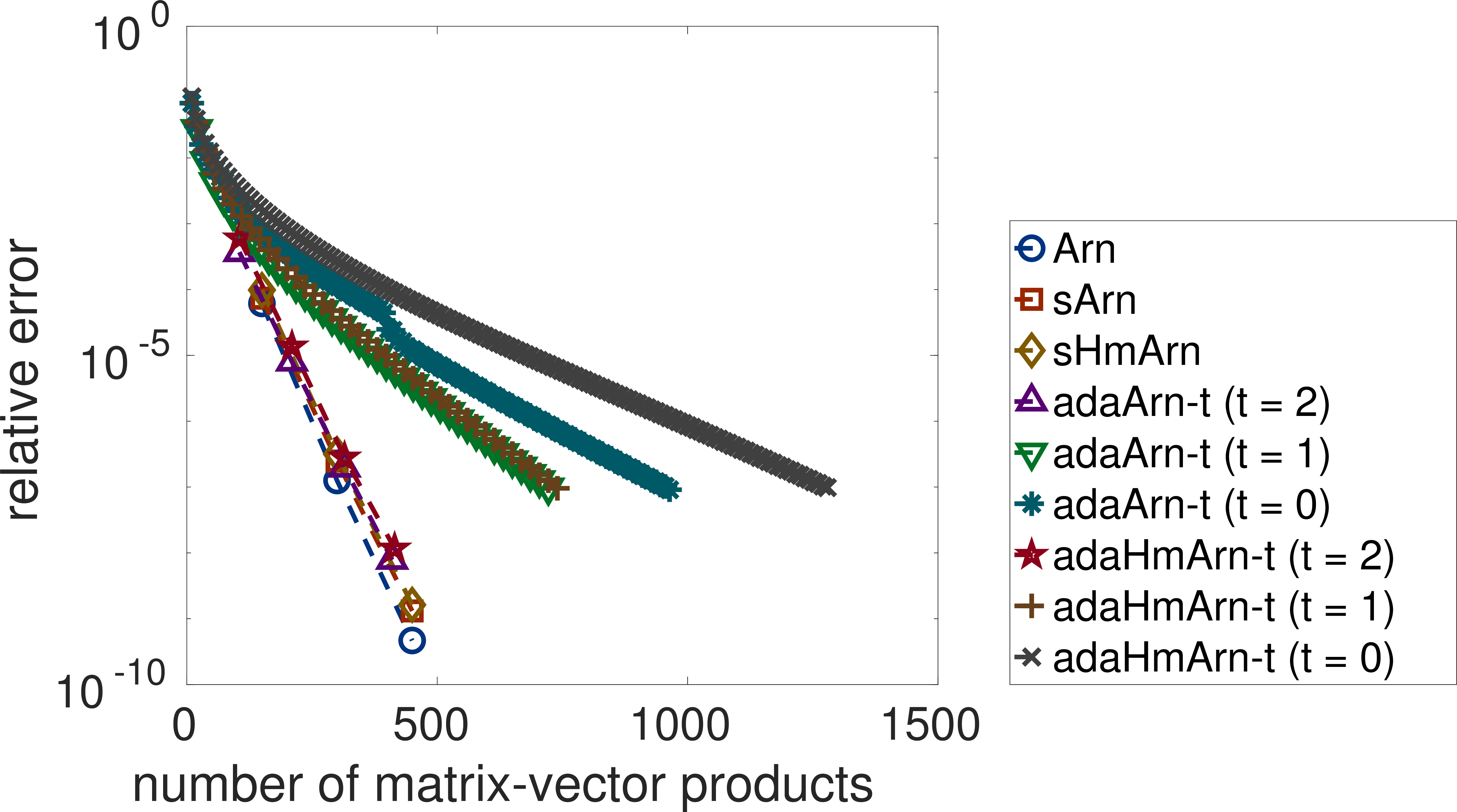
Table 2 and Figure 8 show that all methods attain the prescribed accuracy. The behavior in this example differs from the convection-diffusion problem. Among the fixed-dimension methods, sArn and sHmArn require the same number of restart cycles and matrix-vector products as Arn, but reduce the runtime from \(14\) seconds to \(13\) seconds. This again illustrates the lower per-cycle cost of the sketched orthogonalization process.
For the adaptive methods, \(t = 2\) provides the best overall performance in this example. The methods adaArn-2 and adaHmArn-2 store at most \(105\) vectors, compared with \(150\) for the fixed-dimension methods, while requiring only \(410\) and \(415\) matrix-vector products, respectively. Their runtimes are both \(12\) seconds, which are the smallest among all methods considered. Further decreasing \(t\) substantially reduces the storage requirement, to \(20\) vectors for \(t = 1\) and \(10\) vectors for \(t = 0\), but leads to a pronounced deterioration in convergence. In particular, the number of restart cycles increases to \(40\)–\(41\) for \(t = 1\) and to \(106\)–\(142\) for \(t = 0\), accompanied by a corresponding increase in the number of matrix-vector products and runtime. Thus, for this QCD example, \(t = 2\) offers the best balance among storage, matrix-vector products, and runtime.
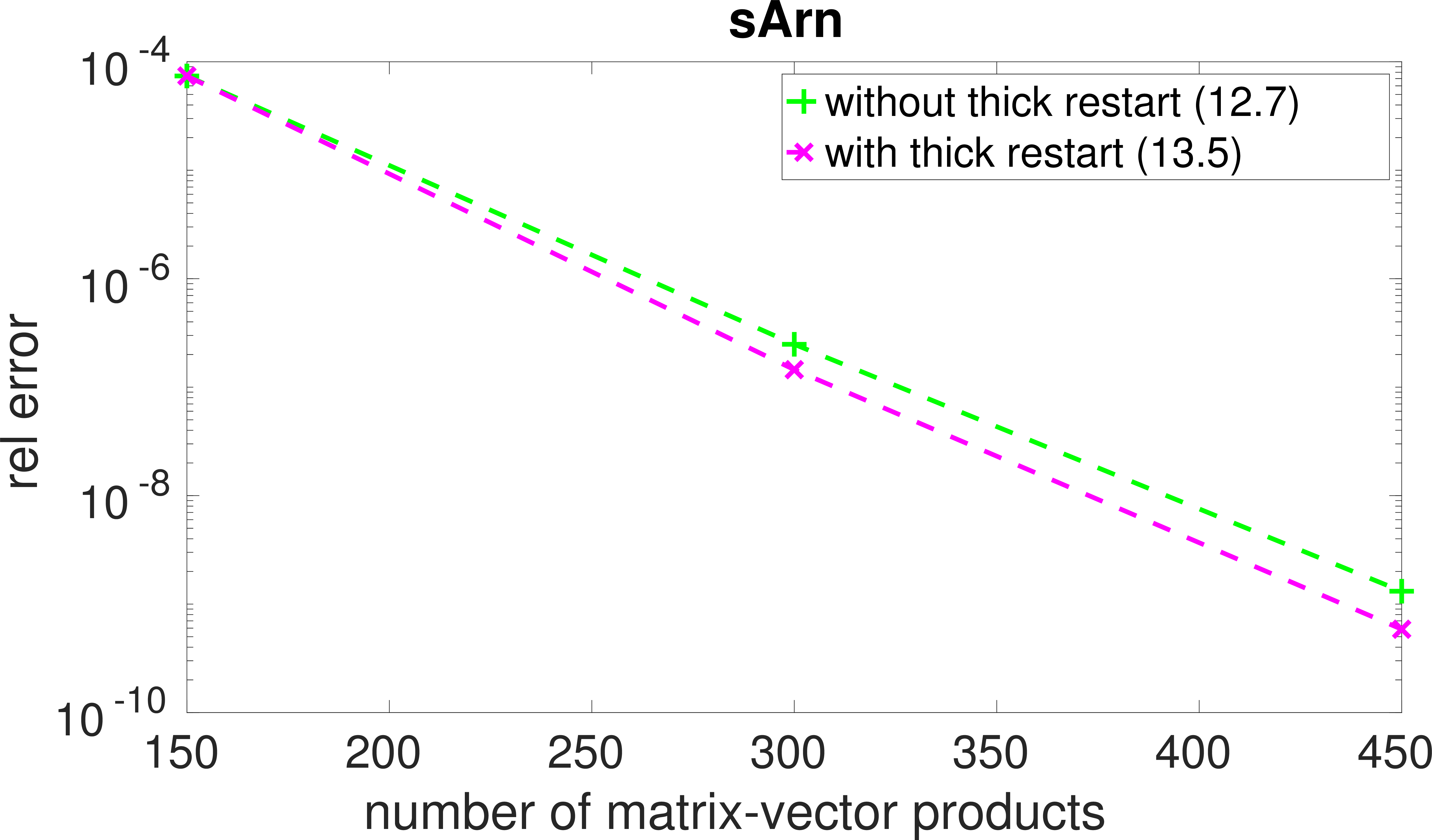
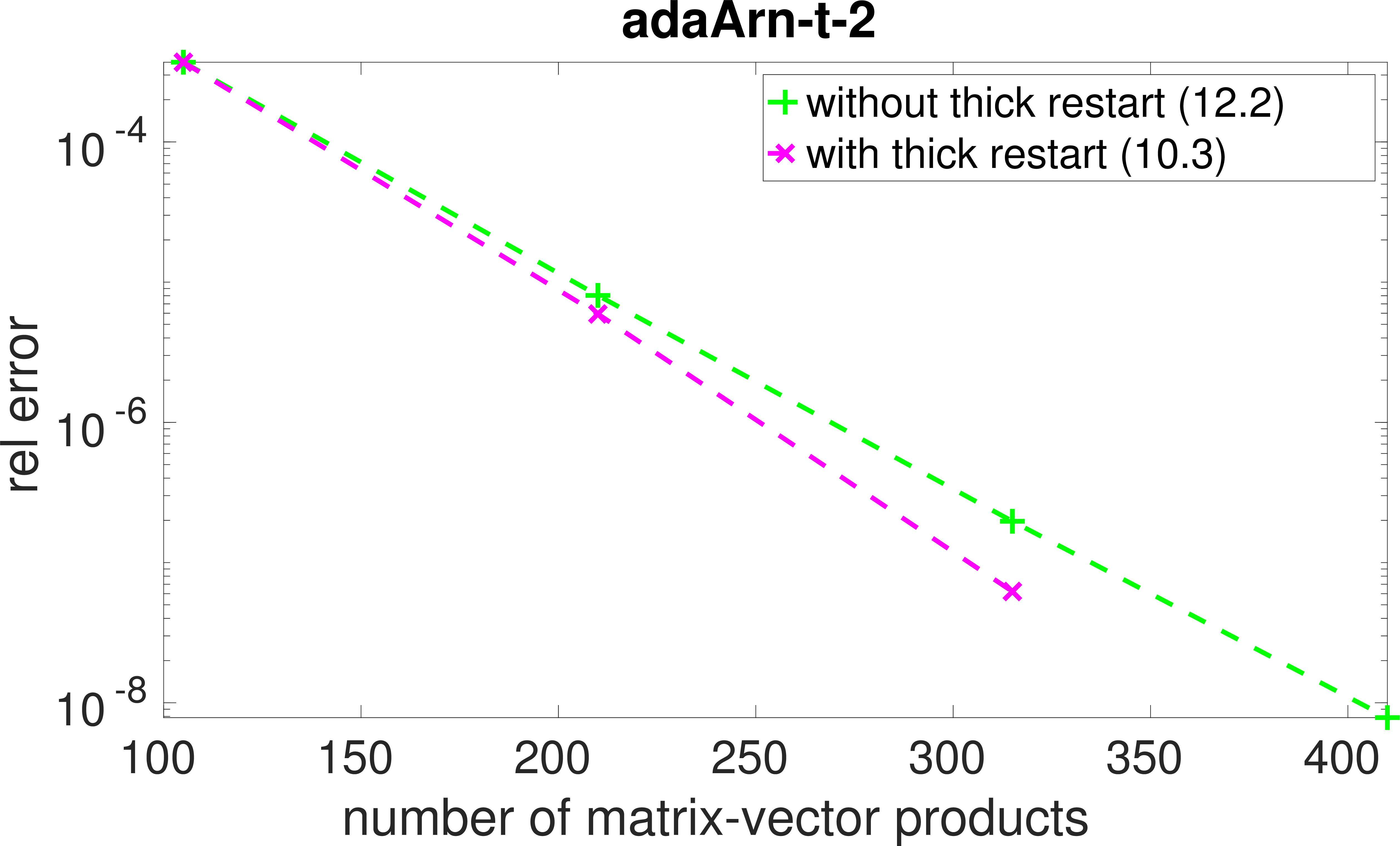
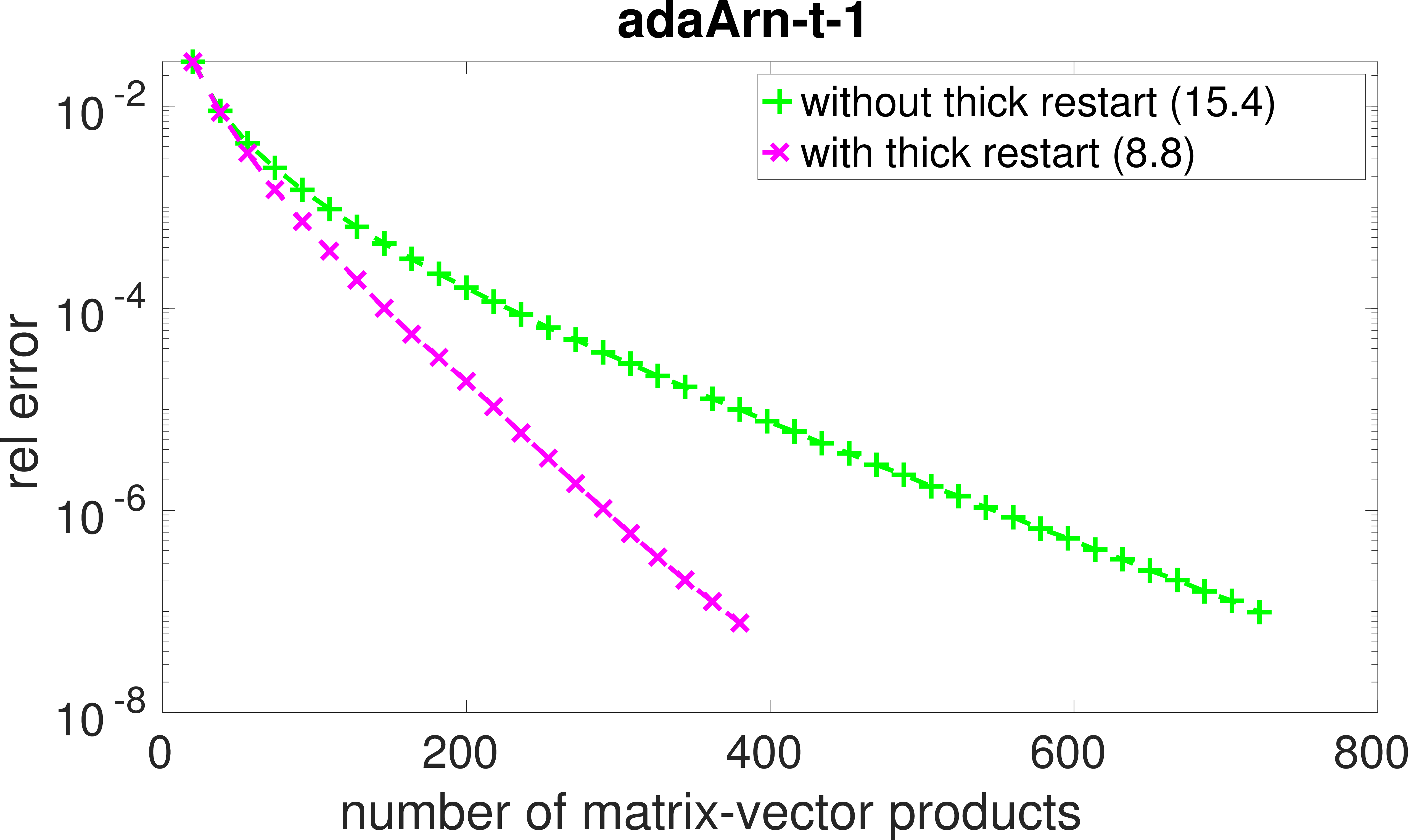
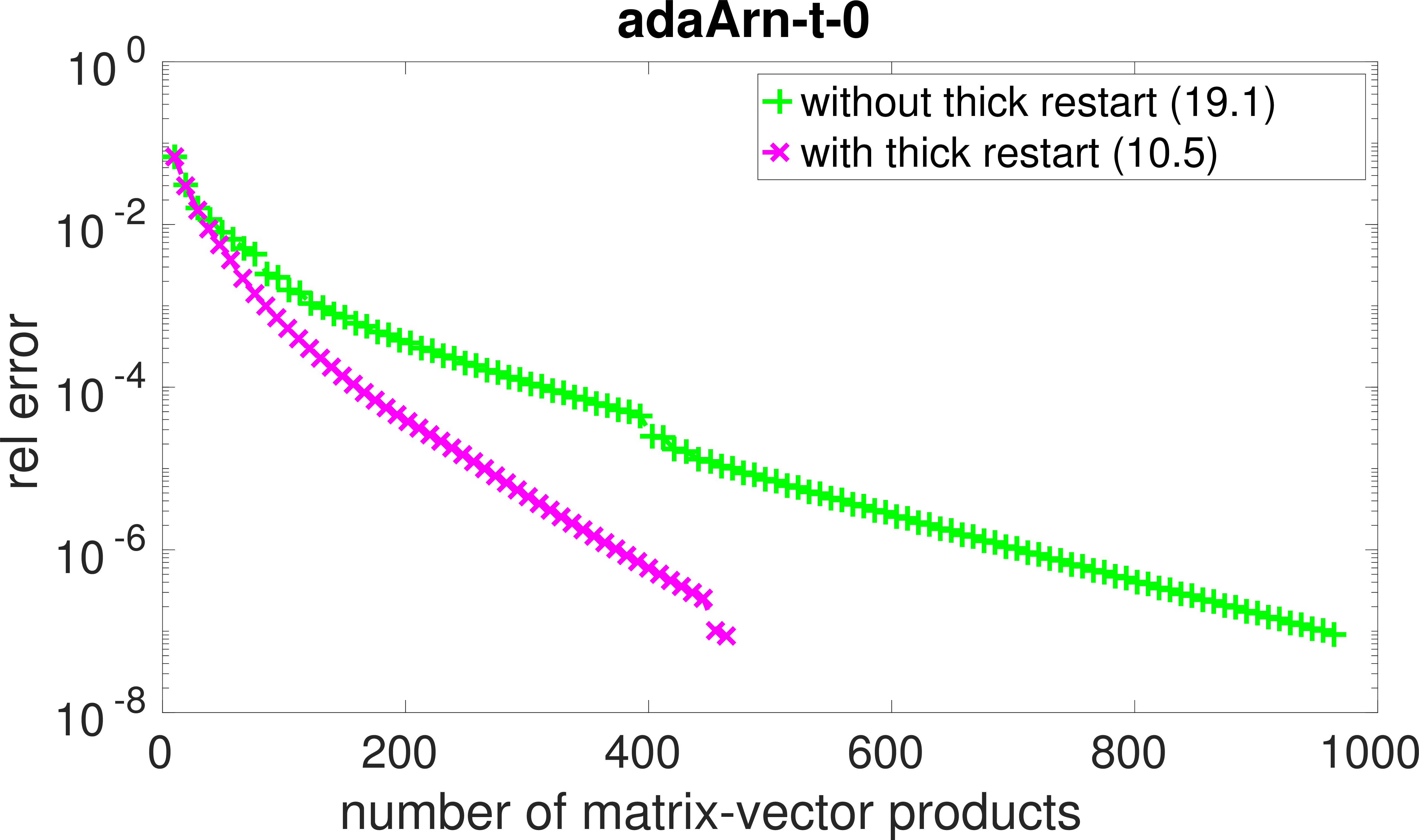
Figure 9: Thick restarting on the QCD example. The runtime of each method is also shown in the legend..
We also apply thick restarting [6] to sArn and the adaptive Arnoldi-type methods, retaining the Ritz vectors associated with the \(5\) Ritz values closest to the origin. As shown in Figure 9, thick restarting has little effect on sArn, whose convergence is already fast; it slightly increases the runtime from \(12.7\) to \(13.5\) seconds. In contrast, thick restarting accelerates all three adaptive methods, with increasingly pronounced benefits as \(t\) decreases. For adaArn-2, the runtime decreases from \(12.2\) to \(10.3\) seconds. The improvement is more substantial for adaArn-1 and adaArn-0, whose runtimes decrease from \(15.4\) to \(8.8\) seconds and from \(19.1\) to \(10.5\) seconds, respectively. These results show that thick restarting effectively mitigates the slower convergence caused by aggressive truncation while retaining the storage savings of the adaptive methods.
6.3 Fractional graph Laplacian example↩︎
In this example, \(\boldsymbol{A} \in \mathbb{R}^{6301 \times 6301}\) is the nonsymmetric adjacency matrix of the p2p_Gnutella08 network from the SuiteSparse Matrix Collection [21]. We define the in-degree graph Laplacian by \(\boldsymbol{L} = \boldsymbol{D} - \boldsymbol{A}\). The matrix \(\boldsymbol{L}\) is singular, and its spectrum lies in the closed right half-plane. We interpret the inverse square root as acting on the invariant subspace associated with the nonzero spectrum and compute \[\boldsymbol{L}^{1/2}\boldsymbol{b} = \boldsymbol{L}^{-1/2}\boldsymbol{L}\boldsymbol{b}.\] Since \(\boldsymbol{L}\boldsymbol{b} \in \mathcal{R}(\boldsymbol{L})\), the Krylov subspace methods
considered here can be applied to this inverse-square-root action. We set \(m = 100\).
| method | error | time (s) | \(n_{\iter}\) | \(n_{\matvec}\) | \(n_{\vecs}\) |
|---|---|---|---|---|---|
| Arn | 4.3e-08 | 8.4e-01 | 3 | 300 | 100 |
| sArn | 4.3e-08 | 4.3e-01 | 3 | 300 | 100 |
| sHmArn | 4.3e-08 | 4.3e-01 | 3 | 300 | 100 |
| adaArn-\(2\) | 8.0e-08 | 4.4e-01 | 8 | 355 | 45 |
| adaArn-\(1\) | 5.5e-08 | 6.2e-01 | 33 | 606 | 30 |
| adaArn-\(0\) | 9.9e-08 | 8.3e-01 | 78 | 785 | 15 |
| adaHmArn-\(2\) | 6.6e-08 | 4.1e-01 | 9 | 395 | 45 |
| adaHmArn-\(1\) | 9.2e-08 | 4.7e-01 | 25 | 495 | 30 |
| adaHmArn-\(0\) | 8.7e-08 | 8.1e-01 | 74 | 745 | 15 |
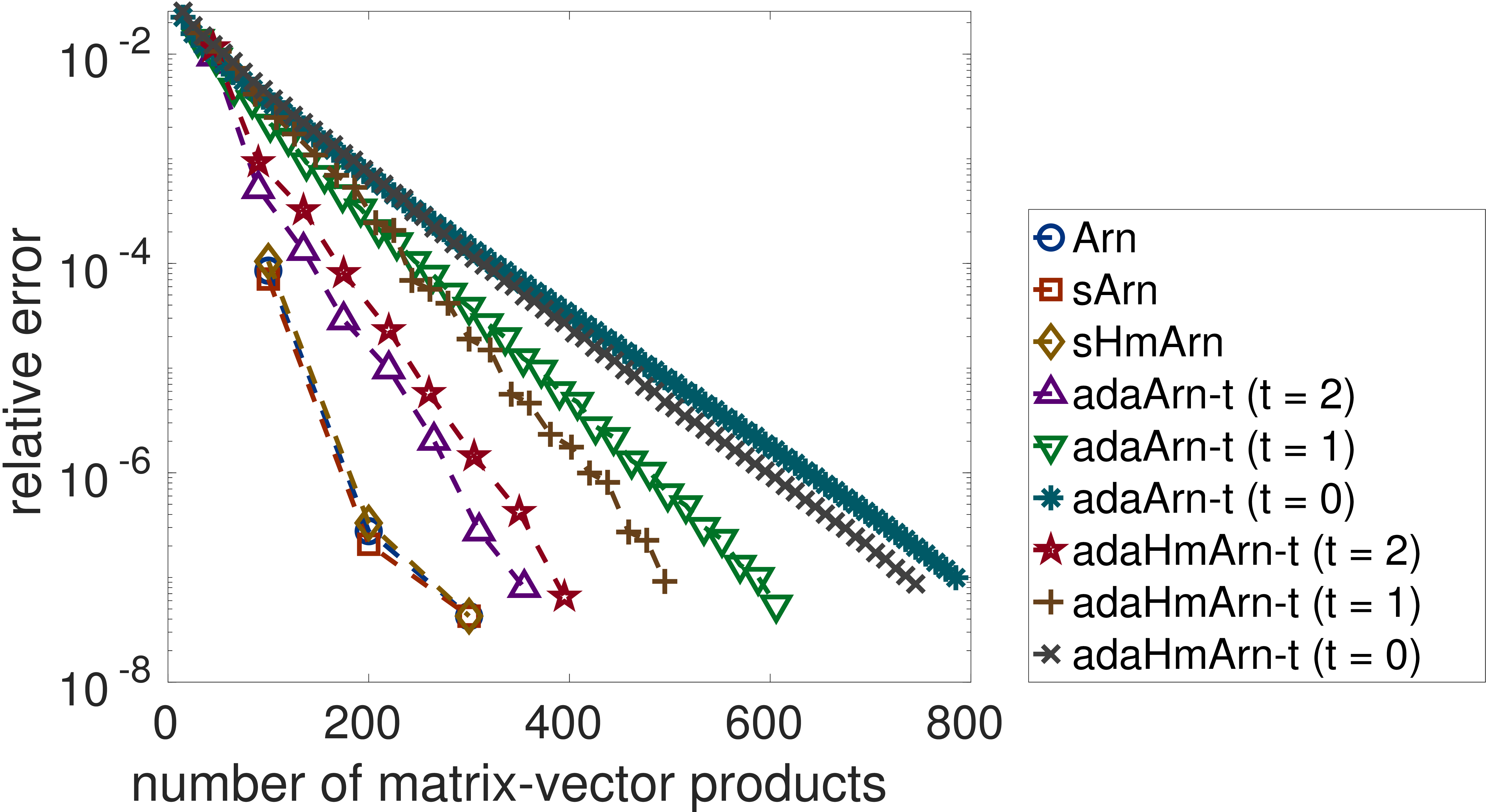
Table 3 and Figure 10 show that all methods attain the prescribed accuracy. Among the fixed-dimension methods, sArn and sHmArn require the same number of restart cycles and matrix-vector products as Arn, but reduce the runtime from \(0.84\) seconds to \(0.43\) seconds. Thus, in this example, sketching nearly halves the computational time without affecting the convergence behavior.
Among the adaptive methods, \(t = 2\) provides the best overall performance. The methods adaArn-2 and adaHmArn-2 store at most \(45\) vectors, compared with \(100\) for the fixed-dimension methods, while requiring \(355\) and \(395\) matrix-vector products, respectively. Their runtimes, \(0.44\) and \(0.41\) seconds, are comparable to those of sArn and sHmArn. Further decreasing \(t\) reduces the storage requirement to \(30\) vectors for \(t = 1\) and \(15\) vectors for \(t = 0\), but substantially slows convergence. In particular, both the number of restart cycles and the number of matrix-vector products increase markedly as \(t\) decreases. Hence, for this example, \(t = 2\) offers the best compromise among storage reduction, convergence speed, and runtime.
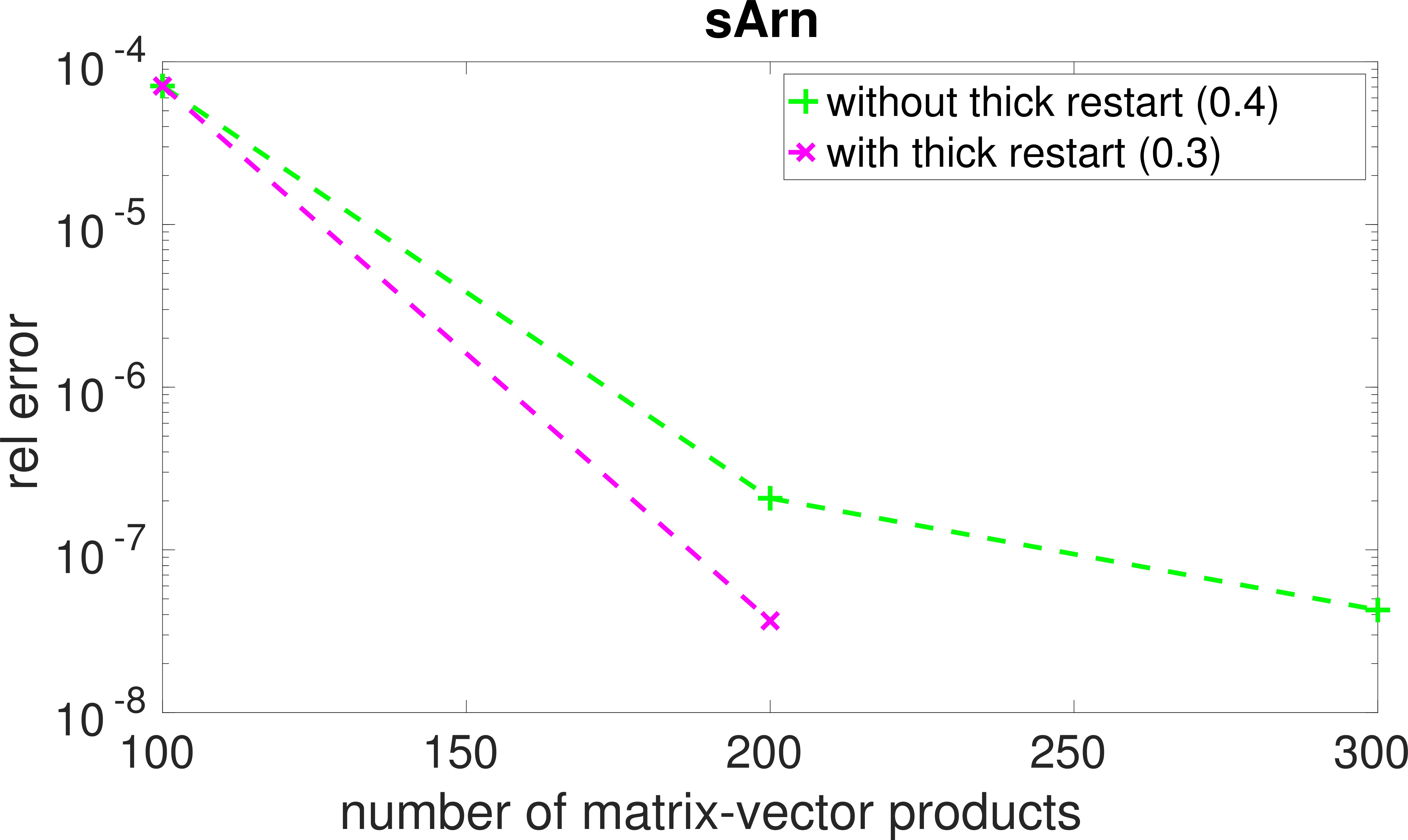
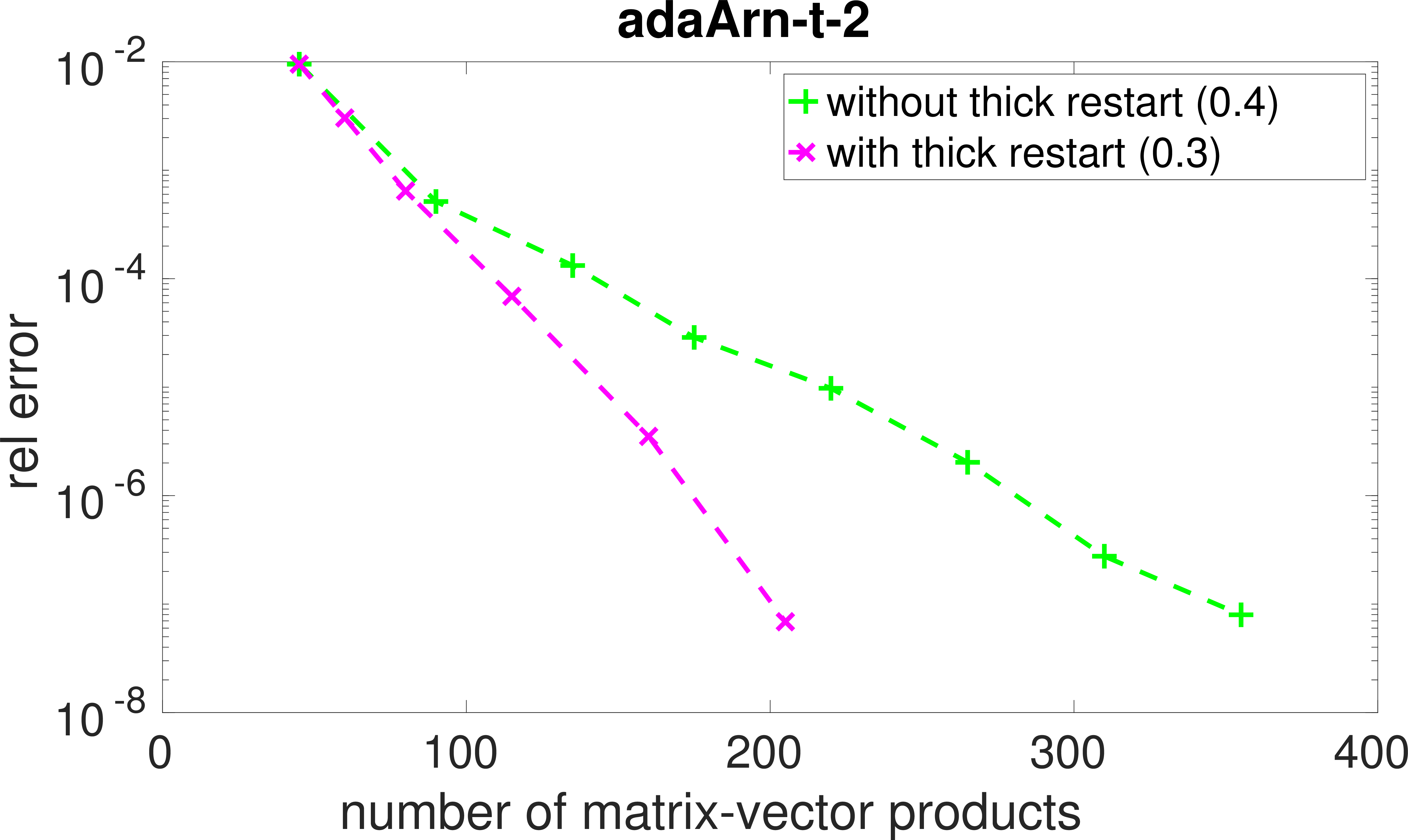
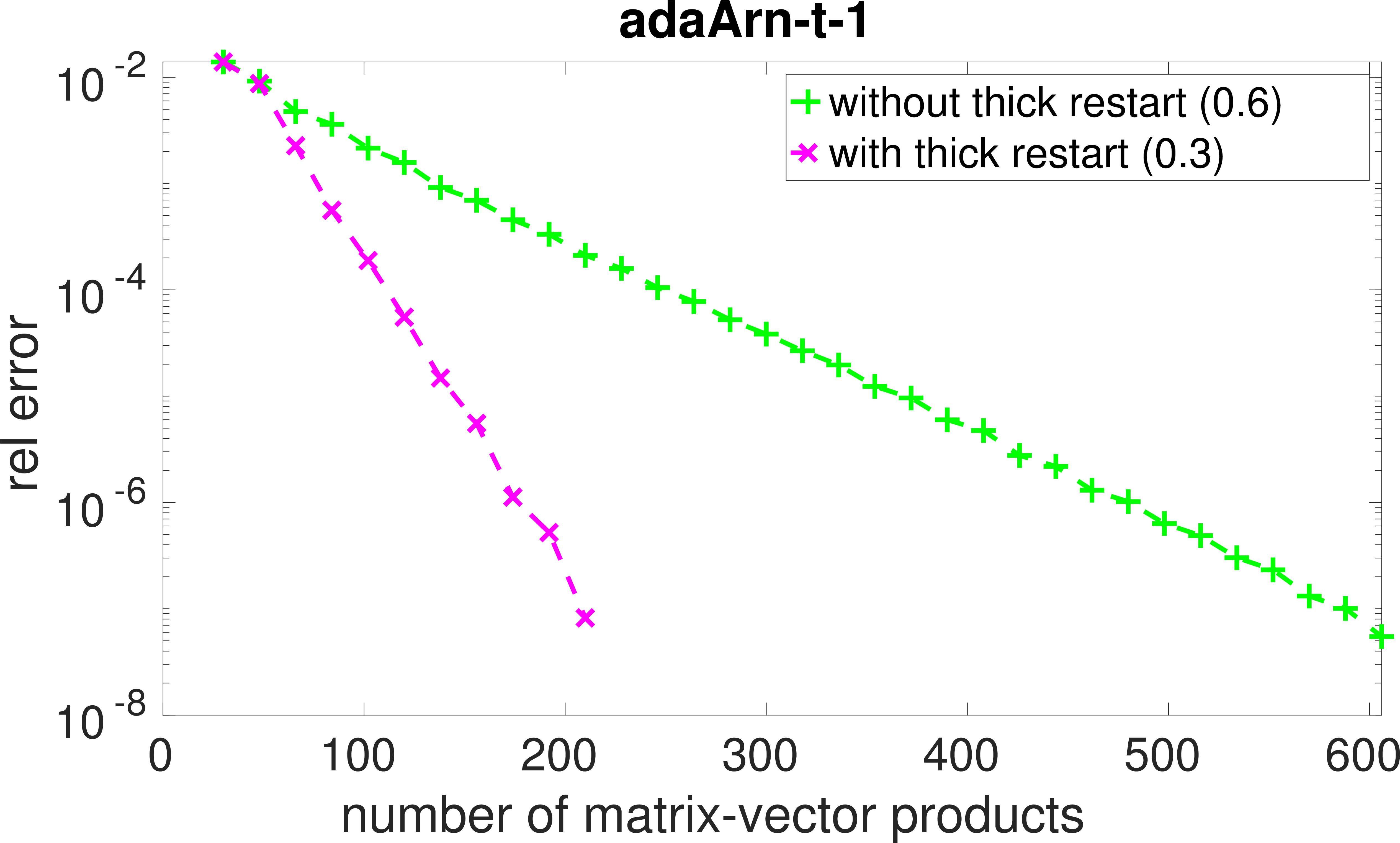
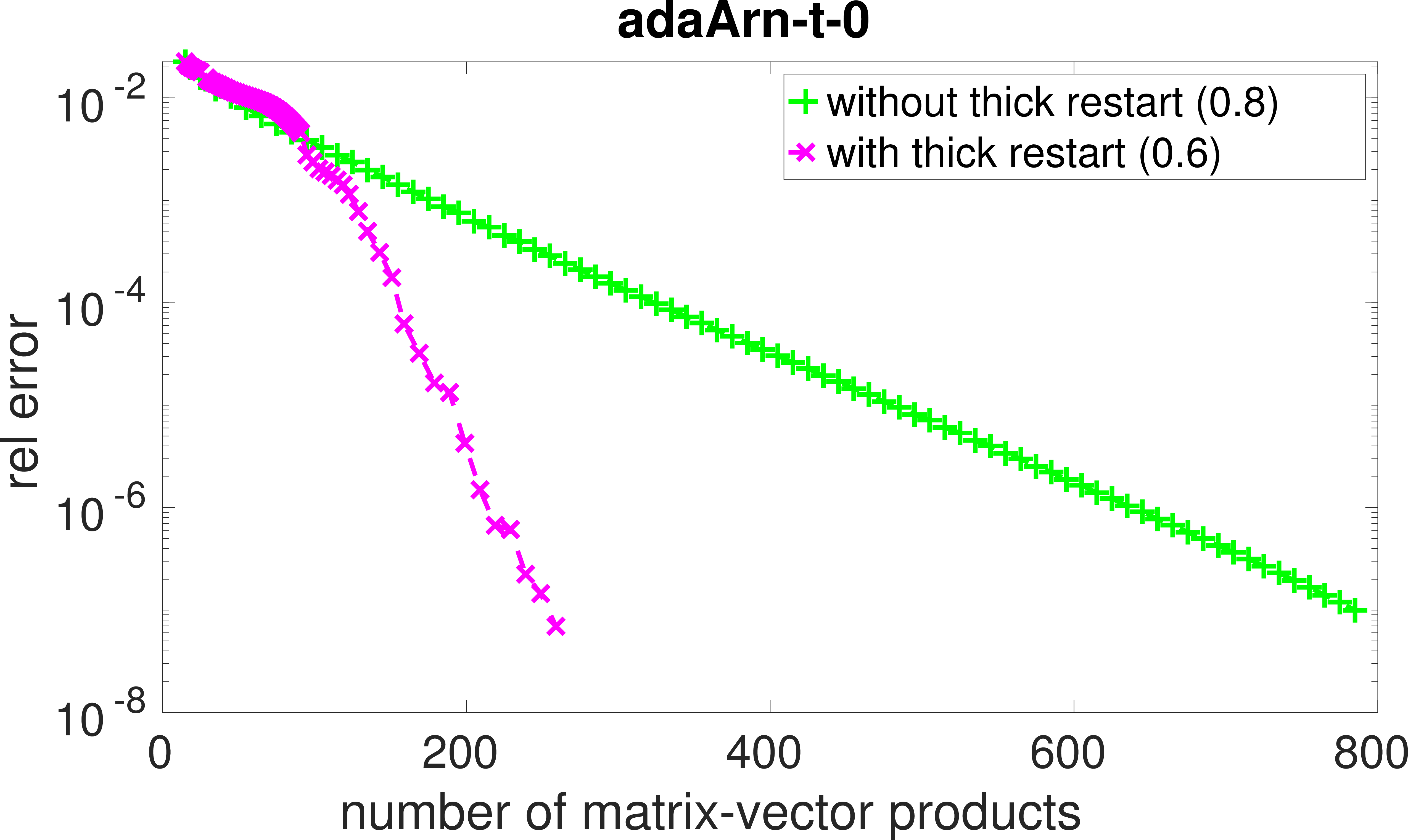
Figure 11: Thick restarting on the fractional graph Laplacian example. The runtime of each method is shown in the legend..
We also test thick restarting with \(5\) retained Ritz vectors. As shown in Figure 11, thick restarting improves both convergence and runtime for all displayed methods. For sArn, the number of matrix-vector products is reduced from \(300\) to \(200\), and the runtime decreases from \(0.4\) to \(0.3\) seconds. For the adaptive methods, the benefits become more pronounced as \(t\) decreases. For adaArn-2, thick restarting reduces the number of matrix-vector products from approximately \(360\) to \(210\) and the runtime from \(0.4\) to \(0.3\) seconds. For adaArn-1, the corresponding reductions are from approximately \(600\) to \(210\) matrix-vector products and from \(0.6\) to \(0.3\) seconds, while for adaArn-0 they are from approximately \(800\) to \(260\) matrix-vector products and from \(0.8\) to \(0.6\) seconds. These results show that thick restarting effectively compensates for the slower convergence caused by aggressive truncation while preserving the storage advantage of the adaptive methods.
7 Conclusions↩︎
We have developed a sketch-and-restart framework for computing \(f(\boldsymbol{A})\boldsymbol{b}\) with large sparse non-Hermitian matrices. The framework combines quadrature-based restarting with Arnoldi-like decompositions generated by sketched or truncated Krylov processes. The key observation is that several Krylov and sketched Krylov approximations share the common form \(\boldsymbol{B}_{m}f(\boldsymbol{H}_{m})\boldsymbol{e}_{1}\beta\), which leads to a unified error representation and restarting mechanism. Within this framework, we combined the existing s-Arnoldi process with quadrature-based restarting and introduced a new sHm-Arnoldi process together with its restarted variant. We further developed adaptive restarted Arnoldi and HmArnoldi methods based on the \(t\)-Arnoldi process and a rank-\(1\) update. For Stieltjes functions, we established the convergence of the restarted sHmArnoldi method when \(\boldsymbol{A}\) is positive real, together with a sufficient condition for the required location of the sketched harmonic Ritz values. More broadly, the proposed framework separates the restarting mechanism from the basis generation procedure, making it possible to incorporate other randomized Krylov processes within the same framework.
Numerical experiments demonstrate the stability and efficiency of the proposed methods. The sketched methods consistently reduce the runtime by lowering the cost of orthogonalization, while the adaptive methods avoid prescribing the restart length \(m\) a priori and can substantially reduce storage. The experiments also demonstrate that thick restarting is an effective complement to aggressive truncation, recovering much of the resulting loss in convergence while preserving the associated storage savings. In particular, the case \(t = 0\) is promising because the inner products required for the rank-\(1\) update can be computed simultaneously at the BLAS-2 level, suggesting that the proposed methods are well suited for high-performance implementations.
Acknowledgments↩︎
JL thanks the China Scholarship Council (CSC) for supporting his visit to The University of Manchester. SG and LN acknowledge funding from the UK’s Engineering and Physical Sciences Research Council (EPSRC grant EP/Z533786/1). SG is supported by Royal Society Industry Fellowship IF/R1/231032.
References↩︎
Department of Mathematics, The University of Manchester, Oxford Road, Manchester, M139PL, United Kingdom,
stefan.guettel@manchester.ac.uk↩︎School of Mathematical Sciences, Fudan University, 220 Handan Road, Shanghai, 200433, China,
jyliu22@m.fudan.edu.cn↩︎Department of Mathematics, The University of Manchester, Oxford Road, Manchester, M139PL, United Kingdom,
lauri.nyman@manchester.ac.uk↩︎