When Does Depth Survive Composition?
Compute–Quality Regimes in Latent World Models
July 11, 2026
Abstract
Adaptive-compute world models—early-exit or mixture-of-depths predictors that spend variable depth per step—rest on two assumptions: that more predictor depth buys better predictions, and that depth can be routed adaptively. In autoregressive rollouts (the planning regime, where the predictor is called many times per encoded observation), the first assumption requires depth’s per-step precision to survive composition. We test this directly. Using a single pre-registered instrument—the shallow penalty \(\rho=\mathrm{err}(\text{shallowest-exit rollout})/\mathrm{err}(\text{full-depth rollout})\)—we classify nine DeepMind Control tasks under matched single-step (\(K{=}1\)) and multi-step (\(K{=}4\) latent-overshooting) training, three seeds each. We find three regimes: on 6/9 tasks depth genuinely helps rollouts (an intrinsic tradeoff, \(\rho\) up to \(4.7\times\)), on 2/9 tasks the shallow exits beat the full stack (inversion, \(\rho\) down to \(0.85\times\)), and one is flat. We then show that the robust inversion (cheetah) is not a property of the dynamics but is created by training: a causal ablation that supervises the early exits only at the first rollout step erases it (\(\rho: 0.87\to1.18\) over \(n{=}8\) seeds, \(\Delta{=}{+}0.31\), distributions non-overlapping), while a task with an intrinsic tradeoff is unaffected—a double dissociation we call the routability catch-22, because the per-step deep supervision that makes early exits usable for routing is exactly what trains them to out-roll the full stack. The mechanism is task-specific: a second, marginal inversion task is unaffected by the ablation. A simple analysis suggests the regime is partly predictable a priori—observation and action dimensionality and one-step model error each correlate with \(\rho\) at \(|\text{Spearman}|\!\approx\!0.75\) (\(n{=}9\)). We also close the loop to control: inside a CEM planner, \(\rho\) predicts whether planning benefits from depth on the tasks where the regime and reward model are robust—most sharply, on the inversion task shallow planning yields higher return than deep. Finally, three cautions for how latent world models are evaluated: a task’s regime depends on the metric space (humanoid is flat in latent space but inverted in observation space), the rollout horizon (the inversion is a short-horizon effect), and the encoder (state-space intrinsic tradeoffs flatten under pixel encoding, one at matched model quality). All thresholds and decision gates were fixed before the compute campaign; the study includes an airtight pre-registered negative for the hypothesis that motivated it.
1 Introduction↩︎
A latent world model encodes an observation to a latent \(z\) and predicts future latents \(z_{t+1}=f(z_t,a_t)\); planning and model-based RL then roll \(f\) forward autoregressively, calling it tens of times per encoded observation [1]–[3]. Because most of a world model’s compute is spent inside these rollouts, adaptive compute—routing predictor depth per step so that “easy” transitions use fewer blocks—is an attractive way to make planning cheaper. This idea inherits the early-exit / mixture-of-depths (MoD) machinery from supervised and language models [4]–[6], and it has an implicit premise: that a deeper predictor produces a better next-latent, so that trading depth trades quality, and a router can pick the depth each step needs.
We ask a prior question that this premise takes for granted: does per-step depth precision survive autoregressive composition? If a \(d\)-block prediction is more accurate than a \(2\)-block prediction for a single step, is the \(d\)-block rollout more accurate than the \(2\)-block rollout after ten composed steps? Only if the answer is yes does routing depth in a planner have anything to route.
We measure this with one number, the shallow penalty \(\rho=\mathrm{err}(\text{shallowest-exit rollout})/\mathrm{err}(\text{full-depth rollout})\) (Section 3). \(\rho>1\) means depth buys rollout quality (a genuine compute–quality tradeoff); \(\rho\approx1\) means shallow matches deep (routing is vacuous); \(\rho<1\) means shallow beats deep (routing deep is actively harmful). Across nine DeepMind Control (DMC) tasks [7], [8], trained with matched single-step and multi-step objectives over three seeds, we find all three outcomes occur, and which one a task exhibits is a stable, measurable property of the (task, training) pair.
1.0.0.1 Contributions.
A pre-registered taxonomy (Section 5). \(\rho\) partitions nine DMC tasks into three regimes—intrinsic (6/9; depth helps, already at single-step training), inversion (2/9; shallow beats deep), and flat (1/9). The intrinsic regime is the majority: for most DMC tasks depth genuinely matters for rollout quality, contradicting the common assumption that latent rollouts are dominated by encoder error.
A causal mechanism for the inversion (Section 6). An ablation that supervises the shallow exits only at the first rollout step erases the inversion on cheetah (\(\rho:0.87\to1.18\), \(n{=}8\)) while leaving an intrinsic-tradeoff task unchanged (double dissociation). The inversion is induced by the training that makes early exits routable—the routability catch-22.
Three evaluation cautions (Section 7). A task’s regime depends on the metric space (humanoid is flat measured in latent space but inverted in observation space), the rollout horizon (the inversion is a short-horizon effect), and the encoder (state-space intrinsic tradeoffs flatten under pixel encoding, one at matched model quality). Latent-space rollout error, the default metric in JEPA-style world-model work, can misstate whether compute helps.
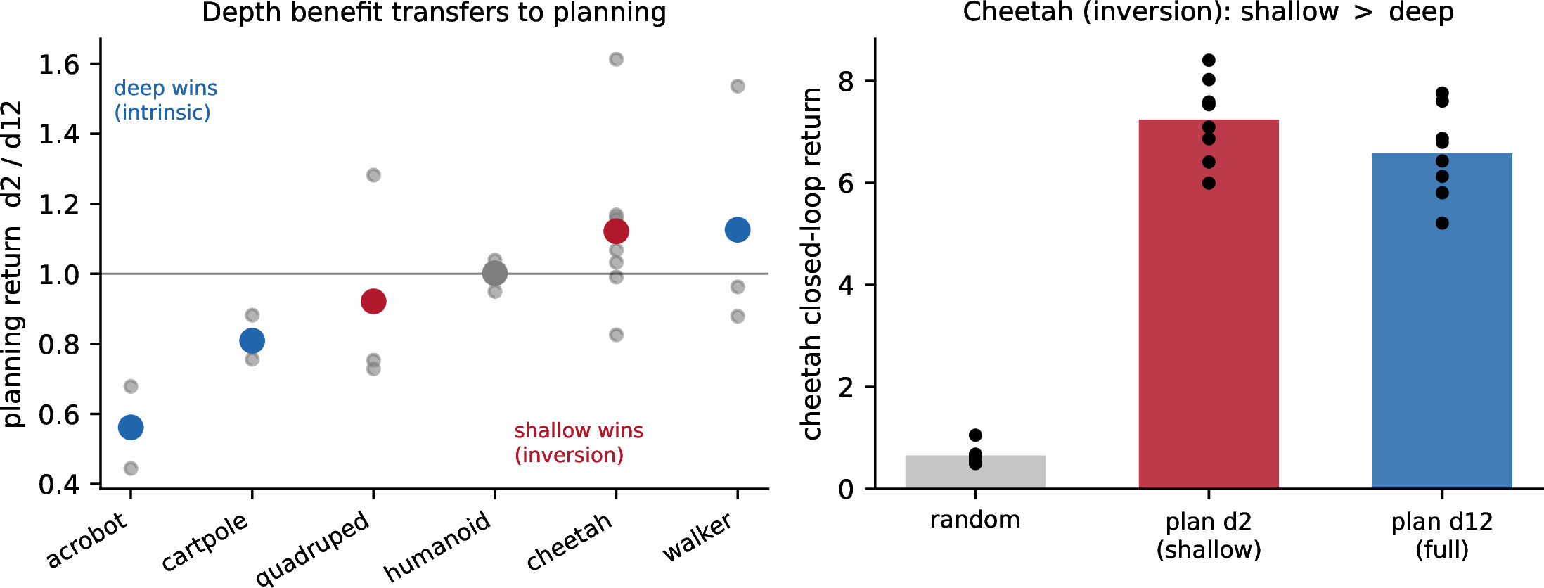
\(\rho\) transfers to planning (Section 9). Inside a CEM planner, \(\rho\)’s sign predicts whether planning benefits from depth—confirmed on two intrinsic tasks (deep helps) and one inversion task (shallow helps), among the four of six tasks with a usable reward model. This validation is partial (two tasks miss, two are reward-unviable) but two-sided, and it converts \(\rho\) from a rollout-error statistic into a control-relevant diagnostic.
Methodology. The entire study is pre-registered: classification thresholds and decision gates were fixed and committed before the compute campaign, and each gate is read once by a mechanical script. This includes an airtight negative for the original hypothesis (Section 4) that reframes, rather than buries, the result.
2 Related work↩︎
2.0.0.1 Adaptive computation.
Early-exit networks [4], [9], [10], Adaptive Computation Time and its successors [5], [11], [12], input-adaptive depth in transformers [6], [13], [14], and sparse mixture-of-experts routing [15], [16] all allocate compute per input in supervised and language models, saving compute at fixed quality (see [17] for a survey). These methods assume a monotone depth–quality relation for a single forward pass. We study whether that relation persists under the autoregressive composition that world-model rollouts require, and find it does not, uniformly—the sign of the depth–quality relation is task- and training-dependent.
2.0.0.2 Latent world models and planning.
World models learn a dynamics function and plan or imagine within it [1], [18]–[20]. JEPA-style latent predictive models [21]–[23] and latent-space planners [3], [24], [25] roll a learned latent dynamics function forward under candidate action sequences. Latent-overshooting / multi-step consistency losses [2], [24], [26]–[28] train the model to predict several steps ahead, precisely to make composed predictions accurate. We use a controlled \(K{=}1\) vs.\(K{=}4\) overshoot as an experimental knob and show that, surprisingly, multi-step training can invert the depth–quality relation on some tasks.
2.0.0.3 Evaluation of latent models.
Latent world models are typically evaluated by latent prediction error against a stop-gradient (EMA) target, following the self-supervised bootstrap of [29] and [30]. We show this choice is not innocuous for compute questions: on one task the depth–rollout regime flips between latent-space and observation-space error, a caution relevant to any latent-space evaluation, and in the spirit of broader calls for evaluation rigor in deep RL [31], [32].
3 Setup and instrument↩︎
3.0.0.1 Model.
We use a block-stacked latent predictor with early-exit heads at depths \(\{2,4,\dots,12\}\) on top of an MLP encoder with an EMA target [29], trained with a latent JEPA loss [22], deep supervision of the shallow exits [33], [34], light distillation toward the full-depth output [35], and VICReg variance/covariance regularization [36] (details in Appendix 13). This is a standard adaptive-compute world-model backbone; our claims concern its rollout behavior, not the specific architecture.
3.0.0.2 The shallow penalty.
For a checkpoint, we encode held-out windows to \(z_0\), roll the predictor \(H{=}10\) steps at each fixed exit depth \(d\), and measure the horizon-mean latent error \(e_d\) against the EMA-encoded true future. The full-depth error \(e_{\mathrm{full}}\) is the denominator and \[\rho\;=\; \frac{e_{d_{\min}}}{e_{\mathrm{full}}},\qquad d_{\min}=\text{shallowest exit},\] with per-depth curves \(e_d/e_{\mathrm{full}}\) retained for shape. \(\rho\) is computed by a single audit script over 256 held-out windows (seed fixed); a collapse guard rejects any checkpoint whose \(e_{\mathrm{full}}\) is numerically degenerate (none were).
3.0.0.3 Compute accounting.
Each residual predictor block (\(d_{\text{model}}{=}256\), MLP ratio \(2\)) costs \(\approx0.26\) MMac; the shallowest exit (depth 2, \(0.57\) MMac) is thus \(\mathbf{5.6\times}\) cheaper than the full stack (depth 12, \(3.19\) MMac). Because the predictor is called once per rollout step while the encoder runs once per real observation, per-step depth routing scales almost linearly with rollout / planning FLOPs. \(\rho\) measures the quality side of this FLOP–quality tradeoff: it is exactly the factor by which spending \(5.6\times\) fewer blocks per step changes rollout error.
3.0.0.4 Multi-step training knob.
We train matched twins that differ only in the training horizon \(K\): \(K{=}1\) (single-step) and \(K{=}4\) (latent overshooting, back-propagating through a four-step full-depth rollout against EMA targets). Both twins draw identical, model-independent, pre-collected data in identical minibatch order, so a \(K{=}1\)/\(K{=}4\) pair differs only in the loss.
3.0.0.5 Pre-registration.
Before running the compute campaign we fixed and committed: the regime thresholds (below), the two decision gates (A, B), a metric-artifact kill criterion, and the precedence rules among them. Each is read once, mechanically, from the persisted JSON. The regime of a task is \[\begin{cases} \boldsymbol{intrinsic} & \rho^{K1}\ge 1.25\\ \boldsymbol{inversion} & \rho^{K1}<1.15 \wedge \rho^{K4}<0.90\\ \boldsymbol{flat} & \rho^{K1}<1.15 \wedge 0.90\le\rho^{K4}<1.25\\ \boldsymbol{created} & \rho^{K1}<1.15 \wedge \rho^{K4}\ge1.25\\ \boldsymbol{boundary} & \text{otherwise,} \end{cases}\] where \(\rho^{K}\) is the three-seed mean at training horizon \(K\). (The created regime—a tradeoff manufactured by multi-step training—was the outcome the study was originally designed to find; Section 4.)
4 The hypothesis that failed↩︎
The study began as a directed test of a specific mechanism. Prior internal results had shown that single-step-trained routers save essentially no compute in rollouts, because shallow and deep rollouts were near-indistinguishable (\(\rho\approx1\))—routing was vacuous. The hypothesis was that this is an artifact of the single-step loss, and that multi-step training would create a depth–quality tradeoff (the created regime): \(K{=}4\) twins would show \(\rho\ge1.25\) while their \(K{=}1\) twins stayed below \(1.15\), on a majority of tasks.
We pre-registered this as Gate 1 (pass iff \(\ge 2/3\) tasks are created) on the three tasks first available (cheetah, humanoid, walker). Gate 1 failed, 0/3. Multi-step training did not manufacture the tradeoff: cheetah inverted (\(\rho^{K4}=0.85\)), humanoid stayed flat, and walker already had a large tradeoff at \(K{=}1\) (intrinsic, not created). A reduced-scale pilot that had shown an encouraging \(1.25\times\) on cheetah collapsed to \(0.85\times\) at full scale—the recurring reduced-scale mirage the full-scale pre-registration was designed to catch. Rather than discard the machinery, we broadened to nine tasks and asked the descriptive question this paper answers: what regimes actually occur, and why?
5 A taxonomy of depth-composition regimes↩︎
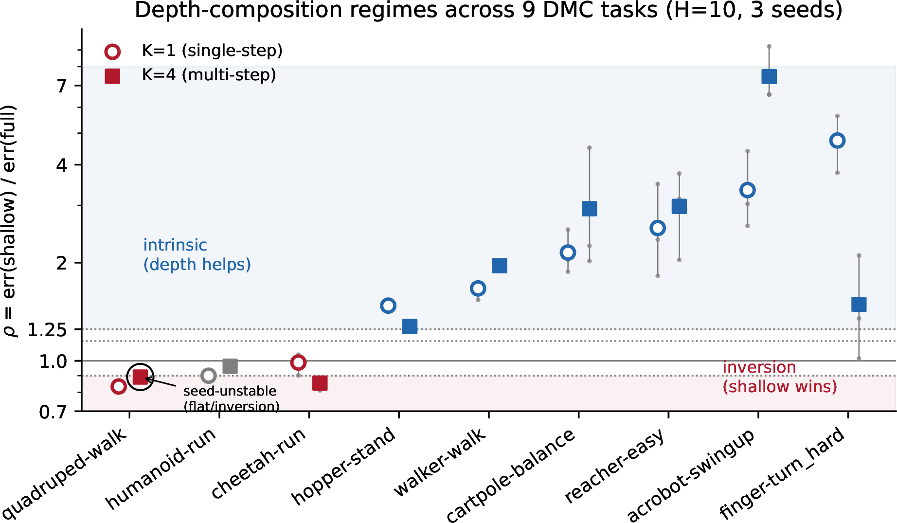
We trained the six additional DMC tasks under the same matched \(K{=}1/K{=}4\), three-seed design (36 runs; all healthy—every checkpoint beats a persistence baseline, none collapsed) and classified all nine (Figure 1, Table 1).
| task | \(\rhov^{K1}\) (min–max) | \(\rhov^{K4}\) (min–max) | regime |
|---|---|---|---|
| finger-turn_hard | 4.74 (3.78–5.64) | 1.49 (1.02–2.10) | intrinsic |
| acrobot-swingup | 3.34 (2.60–4.40) | 7.46 (6.57–9.23) | intrinsic |
| reacher-easy | 2.56 (1.82–3.49) | 2.98 (2.04–3.76) | intrinsic |
| cartpole-balance | 2.15 (1.88–2.53) | 2.93 (2.02–4.51) | intrinsic |
| walker-walk | 1.67 (1.54–1.74) | 1.96 (1.93–2.01) | intrinsic |
| hopper-stand | 1.48 (1.47–1.48) | 1.27 (1.26–1.29) | intrinsic |
| humanoid-run | 0.90 (0.88–0.93) | 0.96 (0.95–0.99) | flat |
| cheetah-run | 0.99 (0.90–1.04) | 0.85 (0.81–0.88) | inversion |
| quadruped-walk | 0.83 (0.82–0.85) | 0.89 (0.87–0.91) | inversion |
| Gate A: PARTIAL — intrinsic 6, inversion 2, flat 1, boundary 0. | |||
5.0.0.1 The intrinsic tradeoff is the majority regime.
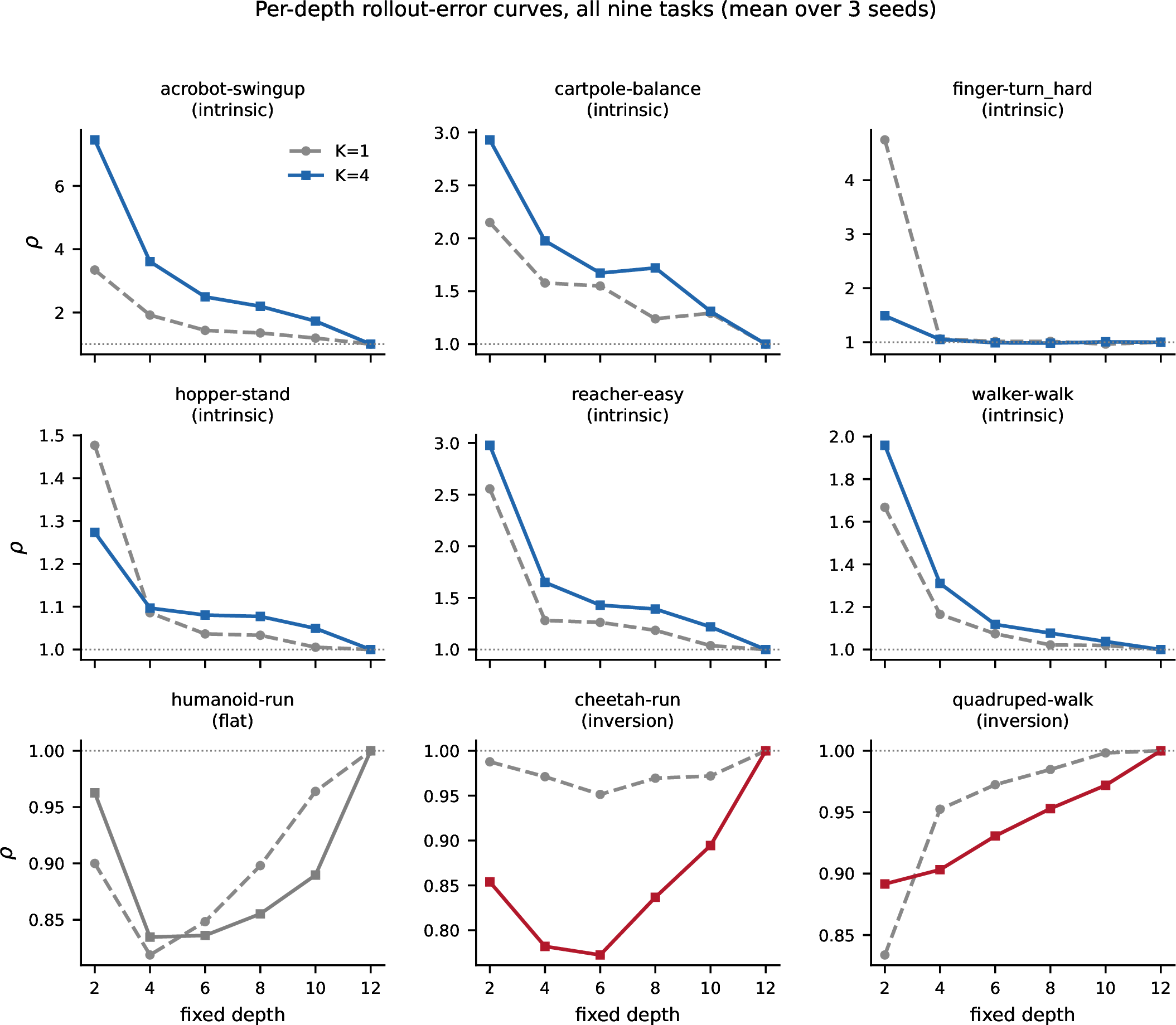
On 6/9 tasks \(\rho^{K1}\ge1.25\): depth buys rollout quality already under single-step training, with no need for multi-step overshoot. This directly recontextualizes the failed hypothesis of Section 4: the premise that “latent rollouts don’t reward depth” was a task-selection artifact of the two tasks first studied. Cheetah and humanoid are precisely the two non-intrinsic outliers; the moment the task set is broadened, depth clearly matters for most of DMC. Multi-step training’s effect on intrinsic tasks is mixed—it amplifies some (acrobot \(3.34\to7.46\), reacher, cartpole) and reduces others (finger \(4.74\to1.49\), hopper \(1.48\to1.27\))—so “train longer horizons” is not a reliable lever on the tradeoff.
5.0.0.2 Seed stability and borderline cases.
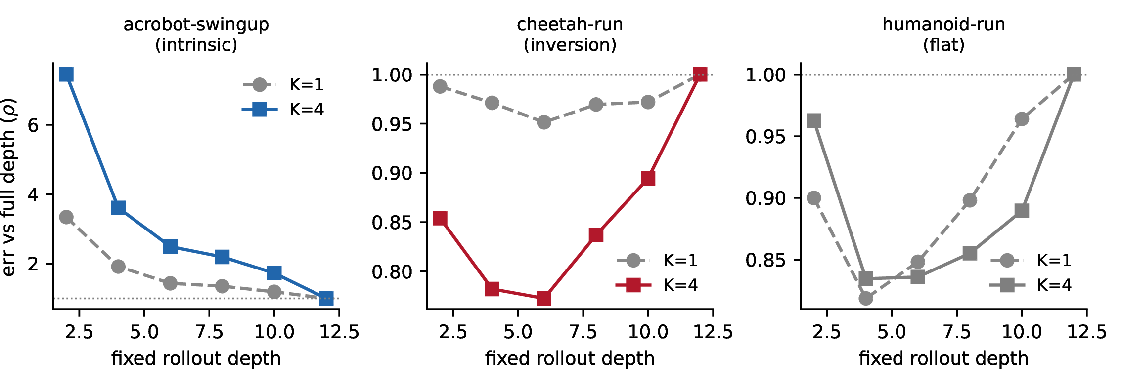
Table 1 reports three-seed means; Figure 1 shows the per-seed spread. Classifying each seed individually, the regime label is stable on 8 of 9 tasks—every seed agrees with the mean label. The sole exception is quadruped, whose \(\rho^{K4}\) sits on the \(0.90\) inversion boundary (inversion under two seeds, flat under one); it is a genuinely borderline inversion, and we treat it as such throughout. Humanoid is the other borderline case: it is flat by \(\rho\) (the ratio at the shallowest exit), but its full depth curve (Appendix 14) dips to \(\approx0.83\) at intermediate depth—inversion-shaped—and its label flips under the metric-space control of Section 7. Cheetah, by contrast, is a robust inversion (all three seeds, both metric spaces, dipping to \(0.73\) at mid-depth); we use it as the primary object of the mechanistic analysis below.
5.0.0.3 Depth-curve shapes.
Figure 2 shows representative per-depth curves (all nine in Appendix 14). In the intrinsic regime the shallowest exit is far worse and error falls monotonically with depth; in the inversion regime the curve dips below 1 at intermediate depths (the full stack is not the best rollout operator); in the flat regime the curve hugs 1 throughout. The full grid also exposes a subtlety behind the metric caution of Section 7: humanoid, labelled flat by \(\rho\) (the ratio at the shallowest exit), in fact dips to \(\approx0.83\) at intermediate depth—its curve is inversion-shaped, and the label is genuinely borderline.
6 The routability catch-22: a causal mechanism for the inversion↩︎
The inversion is counterintuitive—adding blocks makes the rollout worse. Is it a property of the task’s dynamics, or of how we train the exits? Our backbone (like any routable early-exit model) applies deep supervision and distillation to every shallow exit at every rollout step, so that each exit is a usable one-step operator at every point in a rollout. We hypothesized that this per-step composition training is what makes the shallow exits good rollout operators—better than the full stack, which is only ever supervised at full depth.
6.0.0.1 Ablation.
We add a single training flag, deep_sup_first_step_only: when set, the shallow-exit terms (deep supervision + distillation) are computed only at the first rollout step (\(t{=}0\)); the full-depth objective
is unchanged at all steps. The exits remain usable one-step operators but are never composition-trained. We retrain cheetah (inversion) and walker (intrinsic, as a control) at \(K{=}4\), three seeds, and re-audit.
This was pre-registered as Gate B: the cheetah first-step-only mean \(\rho\) must rise by \(\ge0.15\) over the standard \(K{=}4\) mean for
the mechanism to stand.
| task | standard \(K{=}4\) (min–max) | first-step-only \(K{=}4\) (min–max) | \(\Delta\) | \(n\) |
|---|---|---|---|---|
| cheetah-run (robust inversion) | 0.868 (0.81–0.92) | 1.176 (1.06–1.33) | \(\mathbf{+0.31}\) | 8 |
| quadruped-walk (marginal inversion) | 0.892 (0.87–0.91) | 0.843 (0.84–0.85) | \(-0.05\) | 3 |
| walker-walk (intrinsic, control) | 1.959 (1.93–2.01) | 2.064 (2.01–2.13) | \(+0.11\) | 3 |
6.0.0.2 Result (Figure 3, Table 2).
Removing composition training erases the inversion: cheetah’s \(\rho\) rises from \(0.87\) to \(1.18\) (mean over \(n{=}8\) seeds), \(\Delta=+0.31\), with the standard and ablated seed distributions non-overlapping, comfortably passing Gate B. The walker control moves negligibly (\(+0.10\)): a tradeoff that is intrinsic to the dynamics survives the ablation. We call this the routability catch-22: the per-step deep supervision that makes early exits usable for routing is exactly what trains them to out-roll the full stack, removing the depth advantage a router would exploit. Where it applies, making the model routable defeats the purpose of routing.
6.0.0.3 The mechanism is task-specific.
We ran the same ablation on quadruped, the second inversion task. Here it does not erase the inversion: \(\rho\) stays at \(\approx0.84\) (all three seeds below \(0.90\); \(\Delta=-0.05\)). So the catch-22 explains cheetah’s robust inversion but not quadruped’s marginal, seed-unstable one—the two inversions have different origins. This is the honest limit of the mechanism: it is one demonstrated cause of the inversion regime, on its clearest exemplar, not a universal account. (Quadruped’s first-step-only twins were retrained under identical config; its inversion is anyway borderline, Section 5.)
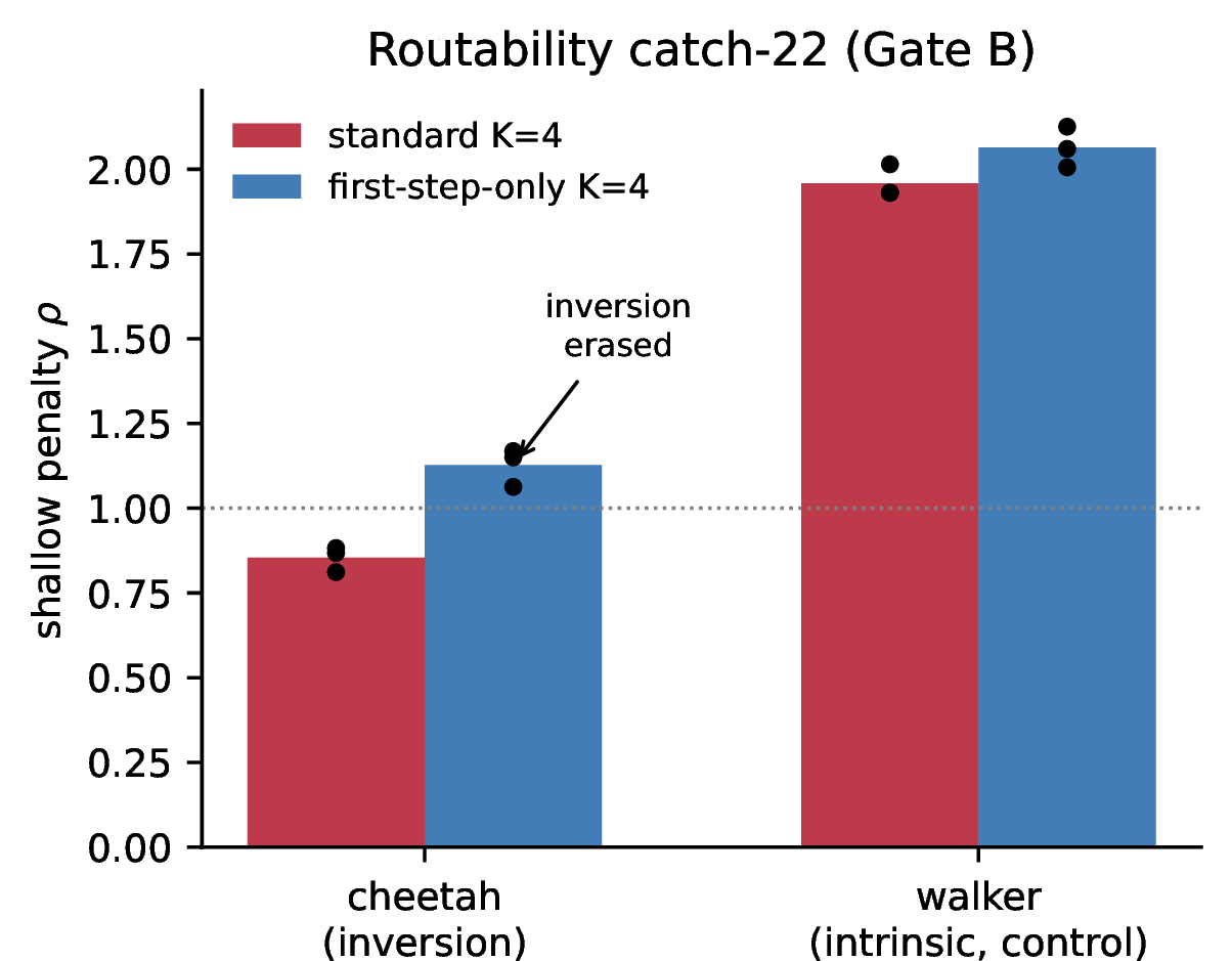
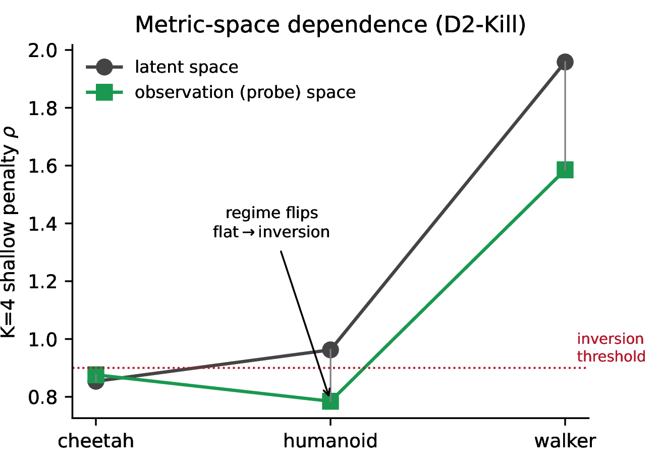
Figure 3: Left: the routability catch-22 (Gate B). First-step-only supervision erases cheetah’s inversion (red\(\to\)blue crosses \(\rho{=}1\)) but leaves walker’s intrinsic tradeoff intact (dots are per-seed). Right: metric-space dependence (D2-Kill). \(K{=}4\) shallow penalty measured in latent vs.observation (probe) space; humanoid’s regime flips flat\(\to\)inversion across the \(0.90\) threshold, while cheetah and walker are stable..
7 Three cautions for evaluating latent world models↩︎
7.0.0.1 Metric-space dependence.
Our \(\rho\) is computed in latent space, the default for JEPA-style models. As a control we fit a linear probe from frozen latents to observations (held-out \(R^2\in[0.95,0.98]\) on all tasks) and recompute the depth curves as observation-space error. We pre-registered a kill criterion: if any task’s regime label changes between spaces, the taxonomy is metric-dependent and must be reported as such. It fired. Humanoid is flat in latent space (\(\rho^{K4}=0.96\)) but inverted in observation space (\(0.78\))—the shallow exits decode to better observations than the full stack, an advantage that the low-variance latent geometry masks (Figure 3, right). Cheetah and walker are stable across spaces. The lesson is general: latent prediction error, the standard world-model metric, can misstate whether compute buys quality, because the encoder’s geometry is not calibrated to observation-space fidelity.
7.0.0.2 Horizon dependence.
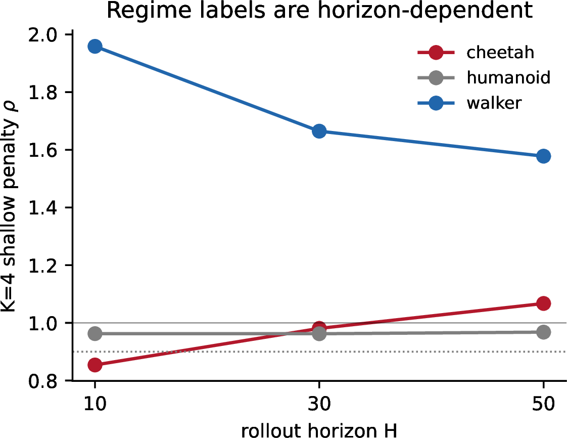
Regime labels are defined at the pre-registered \(H{=}10\). Re-auditing at \(H\in\{30,50\}\) (Figure 4) shows cheetah’s inversion is a short-horizon effect: as the rollout lengthens, the shallow exits’ small per-step errors compound and depth’s advantage recovers (\(\rho^{K4}:0.85\to0.98\to1.07\)). Humanoid (flat) and walker (intrinsic) are horizon-stable. A task’s regime is therefore partly a statement about the planning horizon at which the model is used—short-horizon MPC and long-horizon rollout can sit on opposite sides of \(\rho=1\).
7.0.0.3 Representation dependence.
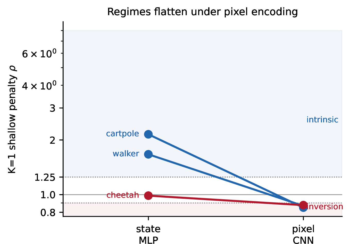
The regime also depends on the encoder. We retrained three tasks from \(64\times64\) pixels with a CNN encoder (K\(\in\{1,4\}\), three seeds; Figure 5). The regimes do not carry over: the two strongly-intrinsic state tasks flatten in pixel space (cartpole \(\rho^{K1}: 2.15\to0.85\); walker \(1.67\to0.87\)), and cheetah’s inversion softens toward flat. Part of this tracks model quality—the pixel cartpole is \(\sim\!600\times\) harder to model, and Section 8 predicts harder-to-model settings flatten—but not all of it: walker’s one-step model error is essentially identical in the two spaces (\(0.0043\) vs.\(0.0044\)), yet its regime flips from strongly intrinsic to flat. The same dynamics, encoded differently, has a different depth-composition regime. The instrument and the phenomenon are not artifacts of a low-dimensional MLP (they behave sensibly on pixel-CNN models), but a task’s specific regime is a property of the (task, training, encoder) triple, not the task alone. (The pixel cartpole \(K{=}4\) was undertrained; we therefore read this comparison at \(K{=}1\), where all six models are healthy.)
7.0.0.4 A null mechanism.
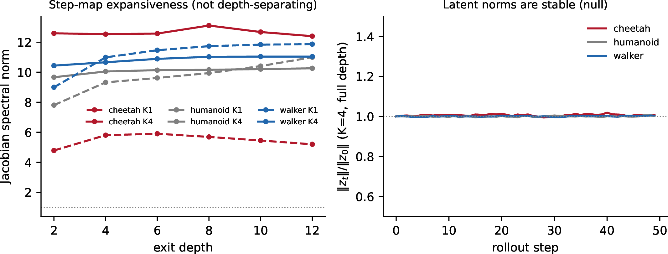
We also asked whether the inversion is explained by contractivity— whether shallow exits have more stable step maps. Measuring exact Jacobian spectral norms and \(50\)-step latent-norm trajectories (Appendix 15), we find latent norms uniformly stable (\(\approx1.0\times\)) and spectral norms that do not separate shallow from deep in a way that predicts the regime. We report this as an honest null: the inversion’s cause is the training effect of Section 6, established causally, not a fixed-point property of the maps.
8 Is the regime predictable a priori?↩︎
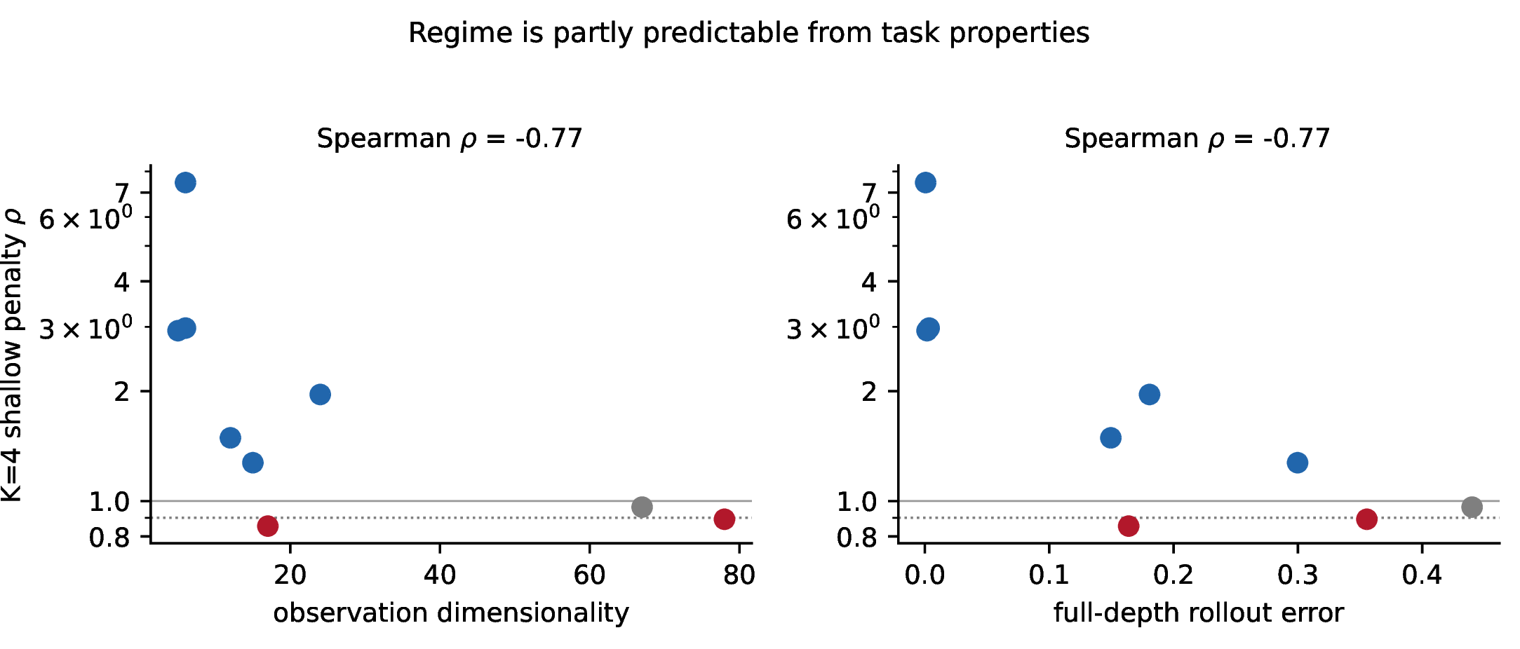
A descriptive taxonomy is more useful if the regime can be anticipated before training a full model. We correlate the nine tasks’ \(\rho^{K4}\) against measurable task/model properties (Figure 6). Three predictors stand out: observation dimensionality (Spearman \(\rho=-0.77\)), action dimensionality (\(-0.73\))—both known a priori from the task—and full-depth one-step model error (\(-0.77\)). The pattern is consistent: the inversion and flat tasks (cheetah, quadruped, humanoid) are the high-dimensional, hard-to-model ones, while the strong intrinsic tasks (acrobot, reacher, cartpole) are low-dimensional and modeled almost perfectly (\(e_{\mathrm{full}}\!\le\!4\times10^{-3}\)). At \(n{=}9\) with predictors that are collinear (dimensionality and model error covary), these are descriptive associations, not a validated predictor—we deliberately avoid partial correlations or significance claims at this sample size. They do, however, suggest a mechanism-level reading worth testing at scale: depth may survive composition when the one-step model is accurate enough that its extra precision is signal rather than compounding noise. On hard, high-dimensional tasks the deep prediction is noisier per step, and that noise compounds into the inversion—consistent with the horizon result of Section 7, where lengthening the rollout eventually restores depth’s advantage even on cheetah.
9 Closing the loop: does \(\rho\) predict planning?↩︎
\(\rho\) is measured from open-loop rollout error. If it is a meaningful diagnostic and not an artifact of that metric, its sign should predict whether planning benefits from depth. We test this directly. On each K=4 checkpoint we fit a ridge reward head on frozen latents (random data plus one on-policy aggregation round; held-out \(R^2\) reported per task) and run a minimal CEM planner (\(256\) candidates, horizon \(10\), 2 iterations) closed-loop on the true environment, at fixed depth 2, fixed depth 12, and difficulty-routed. We pre-registered two predictions before collecting any depth-vs-return data (git history; §3): P1—the sign of \(\mathrm{return}(d_{12})-\mathrm{return}(d_2)\) matches the regime (positive on intrinsic, non-positive on inversion/flat); P2—routed planning reaches \(\ge0.9\times\) the full-depth return at \(\ge25\%\) block savings on intrinsic tasks. A task is viable iff its reward \(R^2\ge0.3\) and the full-depth planner beats random.
9.0.0.1 P1 holds where the regime and the reward model are robust (Figure 7).
The “deep helps” side is confirmed on two intrinsic tasks: cartpole (strong intrinsic, \(R^2{=}0.99\)) where deep planning beats shallow by \(+32\) return, and acrobot (intrinsic, \(R^2\approx 0.70\)) where it beats shallow on both viable seeds (\(+0.4\)). The “deep hurts” side is the sharpest result: on cheetah (robust inversion) shallow planning beats deep (\(7.24\) vs \(6.58\) mean return over \(n{=}8\) seeds, shallow winning on \(6/8\))—the rollout-error inversion reproduces in closed-loop control, the strongest evidence that \(\rho\) is a real diagnostic rather than a latent-metric curiosity. Of the six tasks with a usable reward model, P1 holds on four (cartpole, acrobot, cheetah, and humanoid, whose flat-regime returns are degenerately equal at \(\approx1.0\)) and misses on two—both ones the taxonomy already flagged: quadruped is the borderline, seed-unstable inversion (§5), and walker’s reward model is weak (\(R^2{=}0.55\), noisy returns near \(10\)). Hopper and reacher are filtered as unviable (sparse reward the random policy rarely triggers). So the planning validation is partial but two-sided—\(\rho\) predicts both when depth helps (two tasks) and when it hurts (one task)—and it degrades gracefully exactly where the regime signal or the reward model is weak.
9.0.0.2 P2 fails at the fixed threshold; a calibrated router partly recovers it.
At the fixed default threshold (\(0.5\)), difficulty-routed planning on cartpole saves \(70\%\) of predictor blocks but at \(0.82\times\) the full-depth return—below the \(0.9\times\) bar (P2, pre-registered, fails). We then pre-registered and ran a calibrated router (P2\('\)): sweep the threshold on a calibration set of planning episodes, pick the highest-savings threshold meeting \(0.9\times\) on calibration, and evaluate that frozen threshold on a disjoint set of episodes (no shared seeds; the threshold never sees the evaluation trajectories, so this is not the post-hoc tuning we declined earlier). The calibrated router clears the bar on acrobot for all three seeds—routed return \(1.01\)–\(1.09\times\) full depth at \(83\%\) block savings (routing is essentially free)—and is borderline on cartpole (\(0.80\)–\(0.92\times\), mean \(0.84\), one of three seeds passing). So a leakage-controlled calibration converts the failure on one of the two intrinsic tasks and closes most of the gap on the other; a task-adaptive threshold (e.g.conformal) is the natural next step. The honest reading: \(\rho\) tells you whether depth helps a planner—and on inversion tasks routing deep indeed hurts return—while a properly calibrated router turns that signal into a favorable compute–return operating point on at least some intrinsic tasks.
10 Discussion↩︎
10.0.0.1 Implications for adaptive-compute world models.
Routing predictor depth inside a planner is justified only in the intrinsic regime, where depth buys rollout quality independently of how the exits are trained. That regime is common (6/9 tasks), so the idea is not dead—but it is not universal, and on inversion-regime tasks the standard recipe for making a model routable (per-step deep supervision) trains away the very signal a router needs. A practical consequence: before deploying depth routing, measure \(\rho\); it is a one-script diagnostic that tells you whether routing can help at all, and the first-step-only ablation tells you whether an observed inversion is task-intrinsic or self-inflicted.
10.0.0.2 Implications for latent-model evaluation.
Three of our findings are cautions about methodology rather than about compute per se. Latent-space error can disagree with observation-space error about whether depth matters (metric-space dependence), the answer can flip with the rollout horizon, and it can flip with the encoder (state-space intrinsic tradeoffs flatten under pixel encoding). All three are directly relevant to how JEPA-style models are benchmarked: whether more compute helps is a joint property of task, training, metric, horizon, and representation—not a number one reads off the task.
11 Limitations↩︎
Our study is on state-based DMC with a fixed MLP-encoder backbone. Pixel encoding does shift regime boundaries—demonstrably (Section 7), the intrinsic tradeoffs flatten—so the taxonomy labels are representation-specific; larger backbones may shift them further (the instrument and ablation themselves transfer unchanged). The taxonomy is partial: the flat regime has a single member (humanoid), and—because its latent/probe labels disagree—even that membership is metric-dependent. The pre-registered thresholds (\(1.25/1.15/0.90\)) are reasonable but not derived from first principles; we report raw \(\rho\) values so readers can apply their own. The routability catch-22 is established causally on cheetah (the robust inversion) but is task-specific: the ablation does not erase quadruped’s marginal inversion (Section 6), so it is one cause of inversion, not a universal one. And while Section 8 finds the regime is partly predictable, this rests on \(n{=}9\) correlations with collinear predictors; we have accordingly pre-registered an out-of-sample test (predicting six held-out tasks’ regimes from dimensionality alone, including same-embodiment pairs that must receive identical predictions) whose results will follow. The planning validation (Section 9) is partial: P1 is confirmed two-sided (two intrinsic, one inversion) but misses on the two marginal tasks; the fixed-threshold P2 fails, and a leakage-controlled calibrated router recovers it on acrobot (3/3 seeds) but only borderline on cartpole; and planning on random-policy-trained models is coverage-limited (two tasks unviable). Four concrete next steps our matched-twin dataset is designed to enable: (i) a calibrated router with a threshold selected on held-out episodes disjoint from evaluation (pre-registered here), targeting the P2 return bar we did not clear; (ii) on-policy model training—collecting a single fixed planner-policy dataset and retraining the matched twins on it, to test whether the regime survives the distribution planners actually visit; (iii) a humanoid-style ablation under a representation-robust endpoint (min-over-depths \(\rho\) or observation-space \(\rho\)), since the flat regime has no shallowest-exit inversion for the Gate-B endpoint to erase; and (iv) a larger-backbone replication (\(2\times\) width/depth) to test whether regime boundaries move with capacity.
12 Conclusion↩︎
We asked whether predictor depth survives autoregressive composition in latent world models and answered it empirically, with a single pre-registered instrument, across nine DMC tasks. Depth usually helps (intrinsic, 6/9), sometimes does nothing (flat), and sometimes hurts (inversion, 2/9)—and the inversion is not the dynamics but the training: the deep supervision that makes early exits routable is what trains them to out-roll the full stack. Three evaluation cautions (metric-space, horizon, and representation dependence) round out a picture in which “does compute help?” has a task-, training-, metric-, horizon-, and representation-dependent answer that a simple measurement can recover. The result began as a failed hypothesis and, held to its pre-registration, became a taxonomy, a mechanism, and a set of cautions for a field that has largely assumed the answer.
Reproducibility and pre-registration↩︎
Every number traces to a committed JSON in docs/results/; every figure is regenerated from those JSONs by scripts/make_d2_figures.py. The regime thresholds, Gates A/B, and the metric-artifact kill criterion were committed
before the compute campaign—at git 3462e54 and 935bcb1 (both 2026-07-09), predating the campaign launch commit 387943d—and each is read once by scripts/classify_regimes.py /
scripts/audit_depth_curves.py. The git history provides the timestamped, tamper-evident pre-registration record (an anonymized repository or OSF snapshot can be supplied for review). Two later additions were likewise pre-declared before
running: the seed-count expansion of the headline cheetah comparisons (Gate B \(\Delta\) and planning return) from the campaign’s three seeds to eight was committed at 5efda16 (37 min before the first expanded
checkpoint was written); the calibrated-router protocol P2\('\) with its disjoint calibration/evaluation split was committed at 0995920; and the out-of-sample regime predictor and its held-out predictions
were frozen at 84402b6. The expansion was applied only to the headline task (cheetah); the control tasks (quadruped, walker) remain at three seeds, where their conclusions are already unambiguous—quadruped’s inversion persists on all three
seeds (\(\rho<0.90\)) and walker’s ablation \(\Delta\) is within seed noise. The full chronological record, including the failed Gate 1, the reduced-scale mirage that preceded it, and
these pre-declarations (§§32–38), is in docs/experiment-log.md (§§18–38). Training uses matched, model-independent, pre-collected data so that \(K{=}1/K{=}4\) and standard/ablation twins differ only in their
loss.
13 Architecture and hyperparameters↩︎
Encoder: 2-layer MLP, latent dim 64, hidden 256. Predictor: 12 residual blocks, \(d_{\text{model}} {=}256\), MLP ratio 2, early-exit heads every 2 blocks (depths \(2,4,\dots,12\)), action embedding 64. Loss: latent MSE against an EMA target (momentum \(0.99\)) at full depth; deep supervision of every shallow exit; distillation weight \(0.5\); VICReg variance/covariance regularization. Optimization: AdamW [37], [38], lr \(3\times10^{-4}\), weight decay \(10^{-4}\), batch 256, 60k steps (80k for humanoid), 1000 warmup, grad clip 1. Data: 80 episodes of length 1000 from a random policy per task, collected once per seed. Audits: \(H{=}10\) (\(30,50\) for the horizon study), 256 held-out windows, eval seed 456, probe-fit seed 123. Campaign (91 training runs total): 3 tasks \(\times\,K\!\in\!\{1,4\}\times3\) seeds (original, 18) \(+\) 6 tasks \(\times\,K\!\in\!\{1,4\}\times3\) seeds (breadth, 36) \(+\) first-step-only ablations—cheetah and walker (6) plus quadruped (3)—\(+\) the pre-declared cheetah seed expansion (standard and ablation arms, \(+5\) seeds each \(=10\); Reproducibility) \(+\) 3 tasks \(\times\,K\!\in\!\{1,4\}\times3\) seeds from pixels (18; Section 7). The original, breadth, Gate-B (cheetah/walker), and pixel runs were trained on H100/H200 GPUs (78 runs); the quadruped ablation and the cheetah seed-expansion were trained on an Apple-silicon MPS device (13 runs). Because the expansion adds the same five MPS-trained seeds to both the standard and ablation arms, the Gate-B \(\Delta\) remains hardware-matched within each seed; the quadruped ablation \(\Delta\) carries a Torch-vs-MPS note (Section 6). The planning and calibrated-router experiments (Section 9) are inference-time CEM on frozen checkpoints, not additional training. The pre-registered out-of-sample campaign (36 runs) is pending.
14 All nine depth-curve profiles↩︎
15 Contractivity (null mechanism)↩︎