When Classical Baselines Are Tuned as Carefully
as the Quantum Model, Does Quantum Reservoir
Computing Still Win?
July 10, 2026
Abstract
Can a small quantum computer forecast a changing signal better than an ordinary classical method? Many studies say yes, but the classical methods they compare against are often left in a basic, untuned state while the quantum model is carefully optimised. We ask what happens when the classical competitor is given exactly the same care: the same size and the same amount of tuning effort. We study two popular reasons a quantum reservoir is thought to help, using exact simulations of small quantum systems (up to eleven qubits) on prediction tasks. In both cases the quantum advantage disappears once the comparison is fair. In the first, extra quantum measurements add nothing that a simple classical formula of the same size does not already provide. In the second, a feedback loop genuinely helps the quantum model, turning a useless setup into a working predictor, yet a well-tuned classical network still predicts slightly more accurately, and the gap is statistically reliable. Our point is not that quantum reservoirs can never win, but that two of their commonly cited advantages do not hold up against fair classical competitors at this scale. We provide these matched comparisons as a simple, reusable checklist for honest benchmarking. All results are fully reproducible from fixed random seeds.
1 Introduction↩︎
Reservoir computing [1], [2] trains only a linear readout on top of a fixed nonlinear dynamical system, which makes it an attractive near-term application of quantum hardware: a fixed quantum reservoir avoids the trainability pathologies of variational circuits [3] while supplying a high-dimensional nonlinear feature map. Since the original proposals [4], [5], a growing body of work reports that quantum reservoir computing (QRC) outperforms classical reservoirs and recurrent networks on chaotic, financial, and biomedical time series [6], [7]. At the same time, dequantization and expressivity results [8], [9] caution that the function classes realised by such circuits can often be reproduced classically, which makes the choice of classical baseline decisive.
A recurring weakness in these reports is the classical baseline. When a quantum model is compared against an echo-state network (ESN) [1] or a polynomial readout, the strength of the conclusion depends entirely on whether the classical model was given an equal chance: the same feature-space capacity, the same hyperparameter-tuning budget, the same causal evaluation protocol, and a metric that does not implicitly favour the quantum side. In practice these conditions are often not met. Baselines are reported with default settings while the quantum model is tuned; “classical reservoir” refers to a different architecture than the quantum one; efficiency is measured as simulation wall-clock time rather than any hardware-relevant quantity; and directional accuracy is reported without the persistence control that makes it meaningful.
This paper asks a narrow question: when the classical baseline is matched in capacity and tuning, does the quantum reservoir’s reported advantage survive? We study two representative advantage mechanisms in noiseless statevector simulation at small system size (\(q\le 11\)) and find that on these tasks it does not. Our contribution is not the negative outcome per se but the two controls that produce it: a capacity-matched classical model and a tuning-matched classical recurrent network, together with a correctness-gated, deterministic simulation harness. We state the scope plainly: this is a simulation study at sizes that classical hardware can represent exactly (\(q \le 11\)); the claim is “no advantage here, under fair comparison,” not “no advantage is possible.”
We focus on these two advantage mechanisms because they admit the cleanest matched controls. They are part of a broader fair-comparison cartography of QRC advantage claims: a capacity-matched scaling study of the same reservoir architecture appears in a companion paper [10], and additional angles (high-body trajectory observables, channel-spectrum learning, and cross-asset volatility spillover) are deferred to future work; the methodology and the two controls developed here apply to those settings as well.
2 Methods↩︎
2.1 Common harness and fairness controls↩︎
All experiments share a single evaluation harness with the following properties, several of which are the fairness controls whose absence we are critiquing.
2.1.0.1 Causal, leakage-free evaluation.
Each series is split chronologically into training, validation, and test segments. Every preprocessing step (standardisation) and every hyperparameter is fit on the training/validation portion only and applied causally; the test segment is touched once, for the final reported number.
2.1.0.2 Validation-only tuning, applied equally.
All free hyperparameters (ridge penalty for every method, quantum evolution time \(\tau\), feedback gain \(k_{\mathrm{fb}}\), and the ESN spectral radius and leak rate) are selected by validation error. Importantly, the classical baselines receive the same tuning budget as the quantum model. This is the single most important control and the one most often missing.
2.1.0.3 Matched feature dimension.
Where a quantum and a classical reservoir are compared, their readout feature dimensions are matched so that the comparison is not confounded by readout width.
2.1.0.4 Correctness gates.
Before any result is generated, an automated self-test verifies: the reservoir state is physical (\(\mathrm{Tr}\,\rho=1\) and all measured expectations lie in \([-1,1]\)); the two-point readout computed from the density-matrix diagonal agrees with the explicit operator expectation to machine precision; finite-shot estimates converge to the exact values as the shot count grows; and, for the feedback model, that the feedback path is wired correctly (with gain zero it reproduces the open-loop reservoir to machine precision) and is strictly causal (perturbing a future input leaves earlier features unchanged). Every reported number is read back from disk and checked against a content hash; all results in this paper are deterministic and reproduce bit-for-bit.
2.1.0.5 Metrics.
We report normalised root-mean-square error (\(\mathrm{NRMSE}\), normalised by the per-target standard deviation, so that \(\mathrm{NRMSE}=1\) is the trivial mean predictor) and, for directional tasks, mean directional accuracy (MDA). We define MDA as the fraction of test points on which the predicted direction of the next move matches the observed direction, \(\mathrm{MDA}=\frac{1}{|\mathrm{test}|}\sum_t \mathbf{1}\!\left[\operatorname{sign}(\hat{y}_{t+h}-y_t)=\operatorname{sign}(y_{t+h}-y_t)\right]\), where \(y_t\) is the last observed level. We report it alongside the persistence-MDA: the same directional accuracy achieved by the naive predictor that assumes the most recent observed move continues (\(\operatorname{sign}(y_t-y_{t-h})\)). Persistence-MDA is the meaningful floor for a directional task, since an MDA above \(0.5\) is otherwise easy to obtain on trended data.
2.2 Quantum reservoirs↩︎
The quantum reservoir is a fully connected transverse-field Ising system, \[H = \sum_{i<j} J_{ij}\, X_i X_j + v \sum_i Z_i, \qquad J_{ij}\sim\mathcal{U}[0,1],\;v=1,\] fixed after random initialisation. Classical inputs are angle-encoded via single-qubit \(R_Y\) rotations; the state evolves for time \(\tau\); and the readout consists of single-qubit expectations \(\langle Z_i\rangle\) and, where indicated, two-point correlators \(\langle Z_i Z_j\rangle\), which are estimable from the same computational-basis measurement record [11]. A recurrent variant carries memory across timesteps by partial-tracing the input qubits between encodings, following standard recurrent-QRC constructions [5]. Because \(Z_i\) and \(Z_iZ_j\) are diagonal in the computational basis, all correlators are obtained from the state-diagonal in a single contraction, verified equal to the explicit operator expectation (Section 2).
3 Case study I: a correlator readout adds nothing beyond a capacity-matched polynomial↩︎
3.1 Setup↩︎
A frequently proposed route to quantum expressivity is to enrich the readout with two-point correlators \(\langle Z_i Z_j\rangle\), which capture pairwise quantum correlations and grow the feature space quadratically. The natural question a fair comparison must ask is whether these features carry information that an explicit classical quadratic model does not already have.
We test this on a controlled testbed of \(N=5\) coupled Hénon maps: bounded, genuinely quadratic, multivariate dynamics with a tunable cross-asset coupling \(c\). We compare three models on one-step prediction (all with the same windowed ridge readout and causal protocol): the tuned correlator QRC (\(q=8\), readout tuned over \(\tau\), encoding scale, and single- vs.two-reservoir ensemble); a degree-2 polynomial model (Poly2) whose features are all pairwise products of the windowed inputs, the capacity-matched classical control, given more features than the QRC; and the concatenation \(\mathrm{\small Poly2}\oplus\mathrm{\small QRC}\), which tests directly whether the quantum features add anything to the polynomial basis. Observation noise of standard deviation \(0.1\) is added so that no model can solve the map exactly through its generating polynomial. The concatenation ablation, running the classical and quantum feature sets together and asking whether the union beats the classical part alone, is exactly the control omitted by typical hybrid-architecture reports.
3.2 Results↩︎
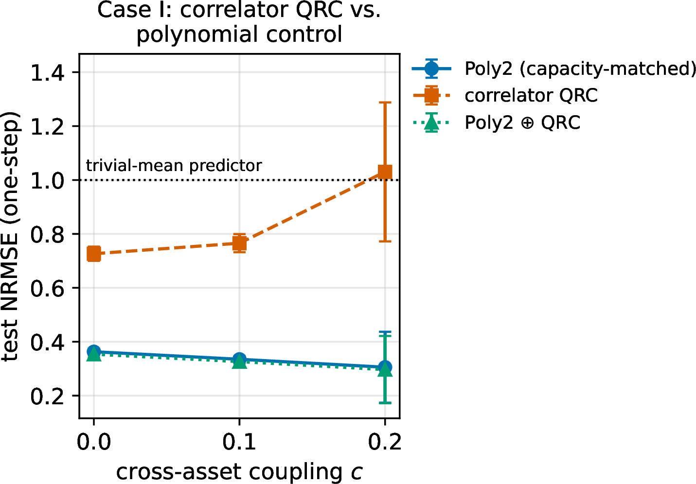
Table 1 reports the verified numbers. At the one-step horizon the Poly2 control beats the tuned QRC outright at every coupling (e.g. \(\mathrm{NRMSE}\) \(0.335\) vs.\(0.766\) at \(c=0.1\)), and at the strongest coupling the tuned QRC degrades to the trivial-mean predictor (\(\mathrm{NRMSE}=1.03\)) while the classical models remain predictive. Concatenating the quantum features onto Poly2 improves on Poly2 alone by only \(\approx\!2.6\%\) at every coupling, the magnitude expected from a few extra mildly-regularising features, not from complementary signal. The same verdict holds on mean directional accuracy: Poly2 reaches \(\mathrm{MDA}\approx 0.96\) (persistence \(\le 0.18\)), the quantum model is no better, and the concatenation does not exceed Poly2. The coupling axis, which one might expect to favour the joint quantum encoding, instead makes the QRC relatively worse (Fig. 1).
| \(c\) | QRC | Poly2 | cat | cat vs.Poly2 |
|---|---|---|---|---|
| \(0.0\) | \(0.726\pm0.026\) | \(0.363\pm0.012\) | \(0.354\pm0.012\) | \(+2.6\%\pm0.3\) |
| \(0.1\) | \(0.766\pm0.034\) | \(0.335\pm0.012\) | \(0.326\pm0.007\) | \(+2.6\%\pm1.5\) |
| \(0.2\) | \(1.030\pm0.258\) | \(0.305\pm0.132\) | \(0.297\pm0.125\) | \(+2.7\%\pm1.0\) |
We are precise about what this does and does not show. The coupled Hénon dynamics are exactly quadratic, so a degree-2 polynomial spans the true generating function class; this is by construction the most favourable possible setting for Poly2, and the result is correspondingly bounded. The claim we make is therefore not “a fair baseline always erases the edge,” but the narrower and fully supported one: when the classical model already covers the data’s function class, a two-point correlator readout contributes nothing beyond it. The concatenation \(\mathrm{\small Poly2}\oplus\mathrm{\small QRC}\) improves on Poly2 by only \(\approx\!2.6\%\) (mean over five seeds, consistent across all three couplings), the magnitude of mild regularisation rather than of complementary signal. The correlator readout does help the QRC relative to a single-point readout, but that gain does not transfer into an advantage over a classical model of matched (indeed larger) capacity. A reader should read Case I as a clean refutation of the specific “correlators add quantum expressivity” argument on quadratic data, not as a universal statement.
4 Case study II: feedback is a live mechanism but loses to a tuning-matched ESN↩︎
4.1 Setup↩︎
A distinct advantage claim concerns feedback-driven QRC, in which the measurement outcome at one step modulates the reservoir drive at the next, making the effective dynamics path-dependent rather than a fixed function of a finite input window. Path-dependence is something a fixed-window polynomial cannot reproduce, but it is precisely what a classical recurrent network also provides. The honest baseline for a feedback reservoir is therefore not a polynomial but a recurrent network, the echo-state network (ESN), and the test is whether quantum recurrence beats classical recurrence at equal tuning.
We use a nonstationary task built so that recurrence is necessary: a hidden two-state Markov process switches the sign of a first-order autoregressive coefficient, so each regime is individually predictable but the regime must be inferred online from the observable history. A correctness gate confirms the task genuinely requires regime inference (an oracle given the hidden state beats a fixed-window linear model, with the gap growing as the switching rate rises). We implement feedback as an additive, saturating term on the input drive angle, \(\phi_t = x_t + k_{\mathrm{fb}}\tanh(\bar m_{t-1})\), where \(\bar m_{t-1}\) is the mean measurement at the previous step; \(k_{\mathrm{fb}}=0\) recovers the open-loop reservoir exactly. We compare, over ten data seeds \(\times\) ten reservoir seeds (\(100\) paired runs; an initial \(3\times3\) grid served only as a pilot), the tuned feedback QRC, its open-loop counterpart, a tuning-matched ESN (spectral radius and leak rate selected on the same validation budget), Poly2, and a linear model.
4.2 Results↩︎
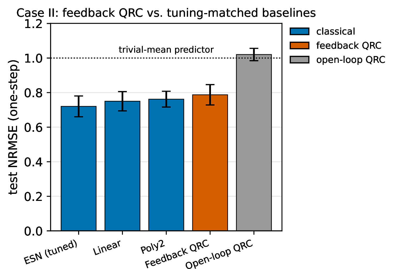
Feedback is a genuine, live mechanism. In the \(10\times10\)-seed comparison at \(p_{\mathrm{sw}}=0.05\) (Table 2, lower), the open-loop reservoir is useless (\(\mathrm{NRMSE}= 1.020 \pm 0.036\), worse than the mean predictor) while closing the loop lifts it to \(0.787 \pm 0.059\), a \(23\%\) improvement on identical seeds. A single-seed switching-rate sweep (Table 2, upper) shows the same effect across \(p_{\mathrm{sw}}\in\{0.02,0.05,0.10\}\) (\(+10\) to \(+19\%\)); we report it as an illustrative trend, with the load-bearing seed-averaged number taken from the lower block. This is, to our knowledge, the clearest case in our study of a quantum reservoir mechanism doing something its open-loop version cannot.
| Upper: feedback vs.open-loop (single seed) | |||
| \(p_{\mathrm{sw}}\) | open-loop | feedback | gain |
| \(0.02\) | \(1.007\) | \(0.874\) | \(+13.2\%\) |
| \(0.05\) | \(1.018\) | \(0.824\) | \(+19.1\%\) |
| \(0.10\) | \(1.032\) | \(0.925\) | \(+10.5\%\) |
| Lower: fair comparison, \(10\times10\) seeds | |||
| method | \(\nrmse\) | MDA | |
| ESN (tuned) | \(0.720\pm0.060\) | \(0.737\pm0.054\) | |
| Linear | \(0.750\pm0.056\) | \(0.735\pm0.055\) | |
| Poly2 | \(0.762\pm0.046\) | \(0.734\pm0.055\) | |
| Feedback QRC | \(0.787\pm0.059\) | \(0.728\pm0.051\) | |
| Open-loop QRC | \(1.020\pm0.036\) | \(0.740\pm0.058\) | |
The mechanism being live, however, does not make it advantageous. Under the fair \(10\times10\)-seed comparison (Table 2, lower), the tuning-matched ESN attains \(\mathrm{NRMSE}= 0.720 \pm 0.060\) against the feedback QRC’s \(0.787 \pm 0.059\), an ESN advantage of \(8.5\%\). Because the \(100\) runs are paired (shared data and reservoir seeds), we test the per-run difference directly: the mean paired difference is \(0.067\) in NRMSE (ESN better), overwhelmingly significant under both a paired \(t\)-test (\(t=12.3\), \(p\approx1.4\times10^{-21}\)) and the Wilcoxon signed-rank test (\(p\approx9\times10^{-17}\)), with a bootstrap \(95\%\) confidence interval of \([0.057,\,0.078]\) that excludes zero. All three of these tests operate across the \(100\) seeds (the across-Hamiltonian distribution): the paired \(t\)- and Wilcoxon tests take the \(100\) per-run ESN-minus-QRC NRMSE differences as their sample, and the bootstrap resamples those same \(100\) paired per-run differences with replacement (\(20{,}000\) resamples), so the interval reflects across-seed/Hamiltonian variability rather than within-run test-point noise. The \(92\%\) figure below is likewise the fraction of the \(100\) paired runs on which the ESN wins. The ESN beats the feedback QRC in \(92\%\) of the paired runs, so the result is systematic rather than driven by a few realisations; and the feedback QRC’s spread across the \(100\) reservoir/data realisations (\(\mathrm{s.d.}=0.059\)) is no larger than the ESN’s (\(0.060\)), confirming the quantum reservoir is not merely an unlucky draw. The feedback QRC in fact trails every classical baseline, including a plain windowed linear model (\(0.750\)); note that on this task the quadratic Poly2 features (\(0.762\)) are themselves worse than the linear model, a reminder that added capacity is not automatically useful. On directional accuracy all models cluster near \(0.73\), far above the \(0.27\) persistence floor but statistically indistinguishable across methods (Fig. 2). The conclusion is that quantum feedback here reconstructs the recurrent memory that a classical recurrent network already provides, and does so slightly less efficiently; closing the loop rescues the quantum reservoir up to, but not past, the classical pack.
5 Discussion↩︎
Two mechanisms, two representative advantage claims, one outcome: under a capacity-matched classical control in the first case and a tuning-matched classical recurrent control in the second, the quantum reservoir’s reported edge does not survive. We emphasise three points.
First, the controls are the contribution. The concatenation ablation (\(\mathrm{\small Poly2}\oplus\mathrm{\small QRC}\) vs.Poly2) directly measures whether quantum features add information to a classical model of matched capacity, and the same-budget ESN measures whether quantum recurrence beats classical recurrence on equal footing. These are inexpensive to run and clear in interpretation, yet they are routinely omitted; including them changes the conclusion.
Second, “live” is not “advantageous.” The feedback reservoir does transform a useless open-loop model into a predictive one. A study that compared feedback QRC only against open-loop QRC, or against an untuned ESN, would have reported a success. The advantage evaporates only against a classical recurrent model tuned as hard as the quantum one.
Third, the scope is bounded and we state it as such. These are statevector simulations at \(q \le 11\), sizes a classical computer represents exactly, on tasks with low-dimensional classical inputs. We make no claim about larger systems, genuinely quantum-state inputs, or non-Clifford resources, where provable learning separations are known to exist [12] and the relevant comparisons may behave differently. Our claim is the narrow, falsifiable one our experiments support: at currently simulable scales, with fair baselines, these two QRC advantage mechanisms do not beat their classical counterparts.
6 Conclusion↩︎
We have shown, under fair comparison, that two representative quantum-reservoir advantage mechanisms, a two-point correlator readout and a feedback-driven reservoir, do not outperform capacity- and tuning-matched classical baselines on the tasks studied, in noiseless simulation at small scale. The two controls behind this conclusion, a capacity-matched classical model and a same-budget recurrent network inside a correctness-gated deterministic harness, are inexpensive, decisive, and routinely omitted; we offer them as a reusable template for honest QRC benchmarking rather than as a verdict on quantum reservoir computing as a whole.
Data Availability↩︎
The result files and the analysis scripts that generate every table and figure in this paper are available at https://github.com/pandey-tushar/Quantum_Chaos_solver (branch
paper-7-cartography). The repository includes the per-seed result JSONs for Case I and Case II, the scripts (mv_correlator_qrc.py, feedback_qrc.py), the figure script (make_figures.py), and a README
mapping each table to the command that reproduces it. All results are deterministic and reproduce bit-for-bit from the provided random seeds.
Acknowledgment↩︎
The author used Claude (Anthropic) to assist with running and optimizing the simulation code. All technical content, results, and conclusions are the author’s own.