Boltzmann MapReduce: A Partition-Function Reduce for Forkable Sandboxes
June 17, 2026
Abstract
To leading order under local asymptotic normality (LAN), the confidence density a worker emits over a chunk of size \(n\) is a Gibbs–Boltzmann measure \(\exp\{-\beta E(\theta)\}\) whose
inverse temperature is the sample size, \(\beta=n\). Three consequences are exact in the Gaussian/linear case and first-order otherwise: disjoint chunks carry independent Boltzmann factors, so the MapReduce reduce,
read literally, is a partition function \(Z=\int\prod_k h_k\,d\theta\) whose mode is precision-weighted (inverse-variance) pooling; frequentist consistency is the zero-temperature limit \(T=1/n\to0\); and the same precision weighting gives pooling an unbounded influence function, so a single “cold” liar reporting false precision hijacks the consensus unless an explicit clip is added. This matters now because the
commodity machine of the AI era is the forkable copy-on-write microVM sandbox. When the unit of execution is a forked ensemble rather than a deterministic path, the reduce should equilibrate that ensemble, not average it. We measure the
statistical core on an open, deterministic (seed \(0\)) reference implementation: the partition-function reduce equals closed-form inverse-variance pooling to machine precision (an algebraic check); the pooled estimate
tracks the full-data oracle to a sampling gap of \(4.3\times10^{-4}\) on a \(12\)-shard mean; the temperature cools as \(1/\sqrt{N}\); a confident liar pulls
the naive pool to \(17.0\) while the clip recovers \(4.95\) and flags it; and on a non-linear, heterogeneous logistic estimator the precision-weighted reduce recovers the full-data MLE while
naive equal-weight averaging is \(\approx\!24\times\) worse (mean over \(8\) seeds). A seven-case pytest suite spanning all experiments passes. We additionally run the
pipeline end-to-end on the islo forkable-sandbox cloud (one trial): a distinct four-shard configuration forked from a \(141\) MB OCI snapshot, each shard computing its density on a separate microVM, reduces to \(4.942\) versus an oracle \(4.945\)—a substrate existence proof (for a fixed shard set and seed the deterministic workers make islo and local outputs identical), and by batching under each
account’s concurrency cap we fork to \(256\)–\(1024\) total sandboxes at \(100\%\) success across three real forkable-sandbox clouds—islo, Daytona,
and Tensorlake (create \(p_{50}\) spanning \(0.20\)–\(6.9\) s). Per-restore microVM latency and large-scale Byzantine accuracy remain projections
from published figures, labeled throughout. Artifact: https://github.com/zozo123/boltzmann-mapreduce.
1 Introduction↩︎
MapReduce did not win on cleverness; it won on fit. Dean and Ghemawat matched a two-primitive model to the commodity machine of their era—the cheap, individually unreliable PC, racked by the thousand—and let the runtime absorb partitioning, scheduling, failure, and communication [1]. The abstraction was canonical because the substrate was: when the unit of hardware is a slow-booting, shared-nothing box, you reduce by summing, counting, and concatenating across them. The arithmetic reduce was a faithful image of the machine beneath it.
The commodity machine of the AI era is a different object. It is the forkable microVM sandbox: a parent boots once, warms its runtime, pauses, and is serialized to a snapshot—an OCI image of content-addressed, deduplicated layers [2]—after which children are cloned not by rebooting but by copy-on-write (CoW) demand paging, each child mmaping the shared backing image and faulting in
only the pages it touches [3]–[5]. Forking a
sandbox is now cheap enough to be a default for real work: running a test suite under many seeds, evaluating a coding agent across parallel rollouts, sweeping hyperparameters, benchmarking a model on sampled shards, or fanning an AI harness over branches
of a decision tree to discard divergent ones [6]. The map step—fork, run, isolate—is commoditized. The reduce step is not.
The trouble is that what these forks emit is noisy and uncertain: a pass rate over flaky tests, an eval score on a sampled suite, a coefficient with a standard error, an agent’s success fraction over stochastic rollouts—each from a different amount of data, each deserving a different amount of trust. The inherited reduce averages and concatenates, discarding exactly the information the ensemble was created to expose: how much data each fork saw, how concentrated its estimate is, and whether one fork’s confident-looking number should move the consensus at all. We argue the reduce over a forked ensemble should be statistical, and that the right statistics fall out of a single observation about what a fork emits.
1.0.0.1 The durable kernel.
Under LAN, the confidence density a worker emits over a chunk of size \(n\) is, to leading order, a Gibbs–Boltzmann measure \(h(\theta)\propto\exp\{-\beta E(\theta)\}\) in which the energy is the local quadratic loss and the inverse temperature is the sample size, \(\beta=n\) (Eq. 2 , Eq. 6 ). A data-poor chunk is hot and diffuse; a data-rich chunk is cold and concentrated. What is empirically falsifiable here is the ratio structure (relative weights track \(n_k\)) and the cooling rate (width \(\sim1/\sqrt{N}\)); taking \(\beta=n\) per observation is the natural convention that makes reduce a partition function. Because disjoint chunks are independent, their factors multiply, so reduce computes a partition function whose mode is precision-weighted pooling; consistency is the zero-temperature limit; and the precision weighting that makes pooling efficient also gives it an unbounded influence function, so a confident liar mandates an explicit clip.
1.0.0.2 What is new.
The divide-and-conquer statistics already exist: parameter servers [7], one-shot [8] and surrogate-likelihood estimation [9], the bag-of-little-bootstraps [10], and confidence-distribution meta-analysis [11], [12]. Our reduce is the Rao-type confidence-distribution (Rao-CD) pooling of Tang and Song [13]; the Gaussian confidence density is textbook LAN. We do not claim these. Our contribution is (i) naming the reduce as a partition function with \(\beta=n\), which makes precision weighting, consistency, and outlier behavior a single thermodynamic statement rather than a family of weighting recipes; and, operationally, (ii) the observation that a cheap forking substrate makes the unit of work a per-shard ensemble of forked replicas rather than one local estimate, and that an arithmetic reduce is no longer the faithful image of that machine.
Contributions.
Identity (proven). The asymptotic confidence density is a Gibbs measure with \(\beta=n\) (Eq. 2 , Eq. 6 ), recasting reduce as a partition-function product (Eq. 7 ) and consistency as the zero-temperature limit, exact under Gaussian/linear energy and first-order otherwise.
Reduce (measured). An open reference implementation: pooling equals closed-form inverse-variance pooling to machine precision; the pooled estimate recovers the full-data oracle; the temperature cools as \(1/\sqrt{N}\); pooling is Byzantine-fragile but clip-repaired; and on a non-linear, heterogeneous logistic estimator pooling recovers the oracle MLE while naive averaging is markedly worse. One end-to-end run on a real forkable-sandbox cloud (islo).
Substrate (enabling design). Forkable CoW microVM sandboxes as the commodity machine that makes the forked ensemble the unit of execution, with a compact agentic control plane and a measured clip as its one validated robustness piece; per-restore latency and large-scale robustness are stated as labeled projections (Tables 2, 3).
2 Programming Model and Forkable-Sandbox Substrate↩︎
The model keeps map/reduce [1] but makes estimates and their variances first-class. The user supplies two
functions; forking, snapshotting, and metadata tracking are abstracted beneath them. map returns, per key, a statistical_result: a point estimate (mean, regression coefficients, empirical CDF), an uncertainty measure (confidence
interval, standard error, sandwich covariance [14], or full confidence density), the local sample size \(n\), and execution metadata. The implemented contract is two calls: a worker emits a confidence-density JSON \((\hat{\theta}_k, J_{n_k}, n_k)\), and reduce_partition multiplies the
Gibbs factors of Eq. 7 —precision-weighted pooling—merging heterogeneous estimates without centralizing raw individual-participant data [12], [13].
2.0.0.1 Worker substrate.
Three properties govern parallelism: instantiation speed, per-worker overhead, and isolation. Containers cold-start in \(0.4\)–\(2\) s with heavy memory overhead; V8 isolates boot
sub-millisecond but cannot run the scientific Python stack. We use lightweight micro-virtualization with memory snapshotting on a minimal VMM such as Firecracker [3], KVM-isolated behind a restricted device model. A parent microVM boots once, warms its runtime, pauses, and is serialized to a snapshot whose information layer is an OCI image: content-addressed base-OS,
runtime, and user-code layers [2], [5] deduplicated and shared read-only
across every fork, so a child is restored rather than rebuilt and only its writes diverge. Each child mmaps its guest memory MAP_PRIVATE and is demand-paged on first touch via userfaultfd [4] with working-set prefetch [15]; a write traps a fault
and copies only that page into a per-child overlay, so shared base layers are never duplicated and disk growth is bounded as fanout rises—a CoW property our local backend exercises directly and the islo run of Sec. 5
exercises on a real cloud. Live branching extends this to running workers: an active worker snapshots in-flight memory and forks a clone with a source-pause window on the order of tens of milliseconds (a reported \(\sim\)56 ms on a \(1.5\) GiB source [6]), the copy completing asynchronously—so an AI
harness can fork at a decision node, test competing branches in parallel, and discard divergent ones. Commercial forkable-sandbox clouds (islo, Daytona [16], Morph [6], Modal) expose this snapshot-and-fork primitive directly.
3 The Boltzmann Reduce↩︎
When the data-generating density cannot be fully specified, inference uses estimating functions built from partial aspects of the mechanism, such as moment conditions [17]. A confidence distribution is a frequentist, sample-dependent distribution encoding confidence intervals of all levels [11], [12]. Processing chunk \(W^{(k)}\), a worker yields a confidence density \(h_k(\theta)\). Under LAN, \[n_k^{1/2}(\hat{\theta}_k-\theta_{k,0})\overset{\text{asy.}}{\sim}N\!\left(0,\,j_k^{-1}(\theta_{k,0})\right), \label{eq:asymp}\tag{1}\] with \(j_k\) the per-observation sandwich (inverse Godambe) information [14], [17]. The confidence density is, to leading order, \[h_k(\theta)\propto\exp\!\left\{-\tfrac{n_k}{2}(\hat{\theta}_k-\theta)^{T}J_{n_k}(\hat{\theta}_k)(\hat{\theta}_k-\theta)\right\}, \label{eq:confdens}\tag{2}\] where \(J_{n_k}\) estimates the per-observation information \(j_k\), so chunk \(k\) carries total precision \(n_k J_{n_k}\). Regime. Under correct specification, \(h_k=\exp\{-n_k E_k\}\,(1+O(n_k^{-1/2}))\); the Gibbs form is exact iff the estimating function is linear in \(\theta\) (Gaussian location, linear regression) and otherwise holds to \(O(n_k^{-1/2})\) by Laplace approximation. Higher-order corrections (skewness, curvature) are exactly what a CD carries beyond first order and are dropped here.
The reduce merges the independent densities via Rao-CD [13], which generalizes MLE to robust estimating equations. With full data one would solve \[\psi_{\text{full}}(W;\theta)=n^{-1}\sum_{i=1}^{n}\psi(W_i;\theta)=0. \label{eq:full}\tag{3}\] Since data cannot be centralized, reduce solves the combined equation for \(\hat{\theta}_{\text{rcd}}\), \[\Psi_R(\theta)=n^{-1/2}\sum_{k=1}^{K}n_k\,S_{n_k}^{T}(\theta)\,\hat{V}_{n_k}^{-1}\,\psi_{\text{sub}}^{(k)}(W^{(k)};\theta)=0, \label{eq:raocd}\tag{4}\] with \(S_{n_k}(\theta)=-\dot{\psi}_{\text{sub}}^{(k)}(\theta)\) and \(\hat{V}_{n_k}\) estimating the sub-estimating-function variance at \(\hat{\theta}_k\). Solving \(\Psi_R=0\) combines local scores, whereas the mode of \(\prod_k h_k\) averages local point estimates; the two coincide exactly only under quadratic (Gaussian/linear) energy, where the score is linear in \(\theta\), and otherwise to first order. Under correct specification and a common truth \(\theta_{k,0}=\theta_0\), Rao-CD is asymptotically first-order efficient, recovering—never exceeding—the infeasible full-data estimator, and dominating equal-weight pooling under heterogeneous information (strictly so when precisions differ; the two agree under equal \(n_k\)), connecting to GMM and quadratic estimating-function optimality [18], [19].
3.0.0.1 The Gibbs view.
Writing the local quadratic loss as an energy, \[E_k(\theta)=\tfrac{1}{2}(\hat{\theta}_k-\theta)^{T}J_{n_k}(\hat{\theta}_k)(\hat{\theta}_k-\theta), \label{eq:energy}\tag{5}\] Eq. 2 reads \(h_k(\theta)\propto\exp\{-\beta_k E_k(\theta)\}\) with \[\beta_k=n_k. \label{eq:beta}\tag{6}\] This is a normalization convention—energy defined per observation—not a discovery: one could absorb \(n_k\) into \(J\) and set \(\beta=1\). What is empirically falsifiable is the ratio structure (relative weights track \(n_k\)) and the cooling rate (width \(\sim 1/\sqrt{N}\)), not an absolute temperature scale. Under the per-observation convention, a data-poor chunk is hot and diffuse, a data-rich chunk cold and concentrated. For disjoint chunks the factors multiply and energies and inverse temperatures add: \[h(\theta)\propto\prod_{k=1}^{K}h_k(\theta)\propto\exp\!\Big\{-\sum_{k=1}^{K}\beta_k E_k(\theta)\Big\}, \label{eq:partition}\tag{7}\] with \(Z=\int\prod_k h_k(\theta)\,d\theta\). (Additivity needs disjoint partitions; within-shard bootstrap replicas are not independent \(\beta=n_k\) replicas and are not multiplied.) The mode minimizes \(\sum_k\beta_k E_k\), i.e.precision-weighted pooling, since chunk \(k\) enters with weight \(\beta_k J_{n_k}\). Statistical optimality is additivity of precisions under the product measure. Robustness to honest heterogeneity is Boltzmann suppression: an honest outlier with modest reported precision is a high-energy, exponentially damped configuration. This is not a Byzantine defense: an adversary reporting false high precision (falsely “cold”) receives large weight and captures the consensus—precision-weighted pooling has an unbounded influence function—which is why the clip of Sec. 4 is mandatory. Separately, fix \(K\) and let every \(n_k\to\infty\) (so \(N=\sum_k n_k\to\infty\)); the per-observation temperature \(1/n_k\to0\) and the measure concentrates by Laplace’s method on the minimizer of the averaged energy, which is consistent for \(\theta_0\) when the estimating function is unbiased with the usual regularity. Frequentist consistency is the zero-temperature limit.
4 Orchestration and Security (Design Sketch)↩︎
The master is replaced by a decentralized, durable agentic control plane (envisioned, not yet measured). The one piece validated below is its core mechanism: a median-absolute-deviation precision clip that caps a confident liar’s reported precision and down-weights location outliers. The remaining design elements are unmeasured. A Command Center receives a high-level JobSpec and realizes it across an agent mesh of planning, execution, and scheduling agents that place work and bridge edge and serverless backends [20]. Agentic workflows break synchronous scheduling, so the control plane runs on durable execution: every hop is logged, an OOM kill or timeout triggers replay rather than a crash, and a failed map task is re-forked from the same base template; the durable log, sharded and replicated, is the component to scale at high fanout. Where a map and its reduce are co-located in a single-address-space tier, software-enforced isolation enables a zero-copy hand-off of the confidence density (reported single-system gains of over \(2\times\) [21] are a design target we do not reproduce). Because nodes span hybrid clouds, vTPM boot-integrity attestation anchors trust before a sandbox joins the mesh (boot integrity only, not statistical behavior), and dynamic information-flow control mitigates co-location side channels. For poisoning, where IID-based defenses such as Krum [22] degrade under non-IID inputs, reduce agents may discard or clip implausibly precise updates; large-scale robustness is left to future evaluation.
5 Evaluation↩︎
We separate what we measured from what we project. The measurements (Sec. 5A) are deterministic (seed \(0\)), Python with only numpy/matplotlib,
and reproduce bit-for-bit from the artifact. The projections (Sec. 5B) are drawn from figures published for the cited systems and from stated design targets; no head-to-head experiment against the named baselines was
run.
A. Measured: the Boltzmann reduce, on real runs↩︎
The implementation realizes Sec. 2 directly: map emits \((\hat{\theta}_k,J_{n_k},n_k)\) and reduce_partition multiplies the Gibbs factors of Eq. 7 . Two backends sit behind one interface: a local backend that forks OS processes, and an islo backend that snapshots a parent microVM once (its environment a
uv-locked Python) and forks one sandbox per shard via the islo CLI (islo snapshot save bmr-base; islo use bmr-shard-\(k\)--snapshot bmr-base ...). We verified
that islo launches a Claude Code harness inside the fork; the deterministic numbers below come from a fixed worker invocation (-- uv run python -m bmr.worker) so the reduce is reproducible.
5.0.0.1 Pooling is the partition function (algebraic); efficiency is recovered (statistical).
On \(12\) homoscedastic shards (\(\mathrm{sd}=1.5\)) with heterogeneous sizes \(n_k\in[107,355]\) around \(\theta=5.0\), the partition-function reduce yields \(\hat{\theta}_{\text{pool}}=4.9542\), CI \([4.8980,5.0104]\), against a full-data oracle \(4.9546\). Two distinct facts: reduce reproduces the closed-form inverse-variance pooled estimator to machine precision—an algebraic check, since multiplying Gaussian factors is that estimator—while the pooled estimator tracks the oracle to a sampling gap \(|\hat{\theta}_{\text{pool}}-\hat{\theta}_{\text{oracle}}|=4.29\times10^{-4}\), a finite-sample efficiency check, attaining the oracle ceiling without exceeding it. The per-shard weights track \(n_k\) exactly as \(\beta_k=n_k\) predicts: the largest shard (\(n=355\)) carries \(12.6\%\) of the weight, the smallest (\(n=107\)) carries \(3.6\%\). The same holds for a \(12\)-shard linear regression (true \(\beta=[1.5,-2.0,0.75]\)): pooled \([1.494,-1.983,0.748]\) versus oracle \([1.516,-1.966,0.730]\), \(L_2\) gap \(3.3\times10^{-2}\). The larger regression gap is finite-sample variation in the design-matrix information across shards, not a failure of the identity; both cases are exactly the linear regime where Eq. 2 is Gibbs-exact, so machine-precision agreement is expected, not surprising.
5.0.0.2 The informative regime: non-linear and heterogeneous.
To test where the identity is only first-order, we run logistic regression—a non-linear estimating function—across five strongly heterogeneous shards (\(n_k\in\{60,120,400,2000,5000\}\), true \(\beta=[0.5,-1.2,2.0]\)). Here the Gibbs energy is the leading-order LAN quadratic, not exact. Across \(8\) seeds the precision-weighted reduce recovers the full-data maximum-likelihood estimator (pooled gap mean \(8.3\times10^{-3}\), sd \(4.2\times10^{-3}\)), whereas naive equal-weight averaging of the per-shard coefficients is mean \(0.18\) away—\(24\times\) worse on average (range \(6\)–\(46\times\) over seeds, scaling with the spread of per-shard information). This is the non-confirmatory result: when shards disagree in size and information, the thermodynamic weight \(\beta_k=n_k\) is what tracks the oracle, and the arithmetic average—MapReduce’s inherited reduce—visibly fails.
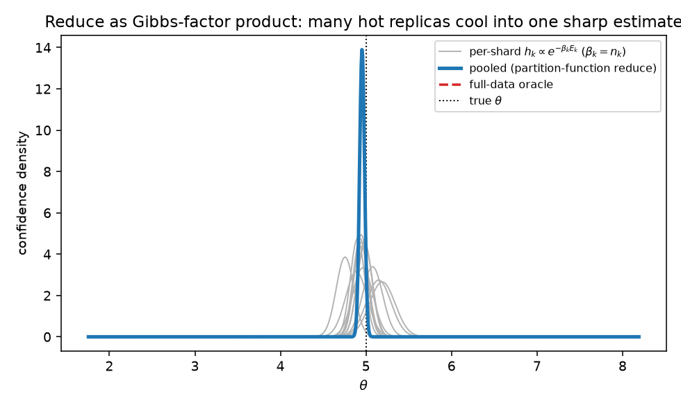
5.0.0.3 Cooling.
As shards accrue, the pooled \(95\%\) CI half-width shrinks while tracking the \(1/\sqrt{N}\) reference in cumulative sample size \(N\)—the zero-temperature limit made concrete: \(T\to0\) as data accrue.
5.0.0.4 Byzantine fragility, and the clip.
Adding to the \(12\) honest shards a single confident liar (\(\theta=17.0\), falsely tiny variance, \(50\times\) inflated precision, fabricated \(n=2000\)), naive pooling is hijacked to \(17.0004\)—the unbounded influence function in action. The detection layer (byzantine_clip, \(\kappa=3\))
caps the liar’s reported precision at \(\mathrm{median}+\kappa\cdot\mathrm{MAD}\); with its fabricated precision capped to the honest scale, its location no longer dominates and the reduce returns to \(4.9542\), matching the clean \(12\)-shard pool, and the liar is flagged. Both halves hold on real data: pooling alone is not Byzantine-robust, and the clip recovers the truth. A seven-case
pytest suite spanning all experiments locks these numbers: the algebraic identity, oracle tracking for mean and precision, regression recovery, clip-versus-liar, JSON round-trip of the Gibbs identity \(\texttt{neg\_log\_density}(\theta)=\beta\cdot\texttt{energy}(\theta)\), and the heterogeneous logistic recovery.
5.0.0.5 End-to-end on a real forkable-sandbox cloud.
We ran the full pipeline on the islo backend in a four-shard configuration: from a \(141\) MB uv-locked OCI parent snapshot we forked one sandbox per shard, each computing its confidence
density on a separate microVM, reducing to a pooled mean of \(4.942\) against a full-data oracle of \(4.945\) (gap \(2.9\times10^{-3}\); committed run log).
Because the workers are deterministic and seed-pinned, for a fixed shard set and seed the islo and local backends produce identical statistical output by construction (this scoping is
why the four-shard islo pair differs from the \(12\)-shard headline run above); the islo trial therefore evidences that the snapshot-once/fork-per-shard substrate executes end-to-end, not that islo yields a
different number. Instrumenting the forks (perf_counter, committed run log), each dispatched in \(\approx\!6.7\) s (min \(6.67\), max \(6.70\)),
with the four concurrent forks completing in \(6.70\) s total. These figures are the restore-plus-run-plus-capture round-trip dominated by client–cloud latency, not the in-host restore (Sec. 5B; see “What we did not do”).
| Cloud | Max fanout | Create \(p_{50}\) | Throughput |
|---|---|---|---|
| Daytona [16] | \(1024\) | \(0.20\) s | \(5.4\)/s |
| Tensorlake | \(256\) | \(3.4\) s | \(0.7\)/s |
| islo | \(256\) | \(6.9\) s\(^\dagger\) | \(1.1\)/s |
5.0.0.6 Fanout, measured on three clouds.
Holding concurrency under each account’s cap and batching, we climb the total fanout from one OCI snapshot on three real forkable-sandbox clouds—islo, Daytona, and Tensorlake (Table 1)—each reaching \(256\)–\(1024\) total forks at \(100\%\) success. Two things stand out. First, per-fork create latency spans nearly two orders of magnitude across platforms exposing the same snapshot-and-fork abstraction (\(0.20\) s on Daytona to \({\approx}6.9\) s round-trip on islo): “forkable sandbox” is one interface but many performance classes. Second, on Daytona create latency is flat from \(64\) to \(1024\) forks—per-fork cost stays bounded as fanout rises. Concurrency itself is account-quota-capped (\({\sim}16\)–\(32\) islo, \(10\) Daytona, \(8\) Tensorlake here), so high total fanout comes from batching under the cap, not raw concurrency—a tier limit, not an architectural one. The statistical ensemble scales identically in the abstract: local process-fork fanout to \(K=1024\) shrinks the pooled \(95\%\) CI half-width from \(0.079\) (\(K{=}16\)) to \(0.0102\) (\(K{=}1024\))—the \(1/\sqrt{K}\) cooling of \(\beta=n\)—with the pooled mean within \(2.1\times10^{-3}\) of the truth (committed run logs).
B. Projected: latency and large-scale robustness↩︎
5.0.0.7 Forking latency.
Our CoW microVM substrate recovers polyglot, KVM-enforced isolation within single-digit milliseconds of isolate-class restore. With snapshot layering and UFFD prefetch [3], [5], [15], published figures suggest low-millisecond restores for a small (\(\sim\)64 MB) working set; a warmed NumPy/PyTorch runtime faults in far more and will exceed this range. Sub-\(20\) ms p99 dispatch assumes a warm-pool hit; a cold miss degrades to the \(100\)–\(150\) ms cold-start row. These caveats hold for the whole row; we do not re-litigate them below.
| Execution Environment | Typical Cold Start | Snapshot Restore (small w.s., proj.) | Language Support | Isolation Depth | Memory Footprint | ||||||||||
|---|---|---|---|---|---|---|---|---|---|---|---|---|---|---|---|
| Traditional Container | 400ms–2000ms | N/A | Polyglot | OS-Level (cgroups) | \(>100\) MB | ||||||||||
| V8 JavaScript Isolate | \(<1\)ms | \(<1\)ms | JS / WASM only | Application-Level | \(\sim 3\) MB | ||||||||||
| CoW MicroVM (Firecracker + UFFD) | 100ms–150ms | 3ms–8ms (proj.) | Polyglot | Hardware/KVM | \(\sim 64\) MB |
5.0.0.8 Large-scale Byzantine robustness.
Under a threat model of up to a \(30\%\) fraction of non-colluding Byzantine workers, our design target is mid-90% accuracy with roughly one-third lower communication than IID-robust baselines, stemming from transmitting condensed confidence densities rather than raw data. This is a design target, not a measurement: we present published Krum/FLAME numbers (Table 3) only as context, on intrusion-detection benchmarks (Edge-IIoTset, CIC-IDS2017, UNSW-NB15) whose protocol and threat model differ from CD aggregation, and we deliberately omit a projected row from the table to avoid implying a head-to-head win we did not run.
| Defense Mechanism | Clean Accuracy | Accuracy under 30% Byzantine fraction | Adversarial Robustness | Comm.Overhead Reduction | ||||||||
|---|---|---|---|---|---|---|---|---|---|---|---|---|
| Krum [22] (published) | % | % | Low | — | ||||||||
| FLAME [23] (published) | % | % | Moderate | % |
5.0.0.9 What we did not do.
We have not run a head-to-head against Krum/FLAME, have not isolated the in-host microVM restore latency (our islo figures are round-trip-inclusive, so the \(3\)–\(8\) ms restore of Table 2 remains projected and is not contradicted by them), reached \(256\)–\(1024\) total forks across islo, Daytona, and Tensorlake by batching under the per-account concurrency caps (tier limits, not architectural) but did not exceed those concurrent caps, and have not validated the LM-agent control plane of Sec. 4. The measured claims are confined to Sec. 5A.
6 Conclusion↩︎
The commodity machine of the AI era is the forkable microVM sandbox, and when the unit of execution is a forked ensemble, the reduce should equilibrate it rather than average it. The kernel is one identity: to leading order under LAN, the confidence density a worker emits is a Gibbs measure with \(\beta=n\), so reduce is a partition function, consistency is the zero-temperature limit, and a confident liar—a falsely cold report—is the failure mode that mandates a clip. We measured this core on an open artifact (Sec. 5A): pooling equals the partition function and recovers the full-data oracle (gap \(4.3\times10^{-4}\)), the temperature cools as \(1/\sqrt{N}\), the clip repairs the Byzantine fragility, and the pipeline runs end-to-end on a real forkable-sandbox cloud. The substrate’s per-restore latency and large-scale robustness remain labeled projections, to be established by systems experiments at scale.
6.0.0.1 Outlook: distributed software engineering for AI coding agents.
We close by naming the larger program this paper opens, as an agenda rather than a measured result. MapReduce gave distributed data a faithful primitive; what is still missing is the analogue for distributed code—a theory and paradigm for code evolution via snapshots, now that the commodity machine is a forkable sandbox rather than a racked PC. The picture is an army of coding agents that fork warm OCI snapshots per task, branch, or hypothesis, evolve code fire-and-forget, and are reaped; the reduce that turns the noisy outcomes these forks emit (test pass-rates, eval scores, build and patch successes, benchmark deltas) into a trustworthy decision has no principled foundation yet. We do not benchmark that program here and claim no software-engineering results for it; our measurements concern only the statistical reduce. What this paper contributes is a first principled primitive for that reduce: each agent’s outcome carries an implicit confidence—how much it ran, how concentrated, how trustworthy—so the right combination is the partition-function, precision-weighted reduce with a Byzantine clip, not an arithmetic average.