Ablation, Statistical Inference, and Validation for KV-Cache Compression
June 14, 2026
Abstract
We present a systematic comparative study of two families of KV-cache compression schemes: TurboQuant (TQ), which applies a randomized Walsh-Hadamard rotation and a data-oblivious Beta Lloyd-Max codebook, and SpectralQuant (SQ), which calibrates a per-head eigenbasis and allocates bits via water-filling. Both families optionally append a 1-bit Johnson-Lindenstrauss (QJL) residual sketch on the key path, the value path, or both.
We make three contributions. First, we perform a full ablation across multiple QJL variants and embedding dimensions, and show that only three schemes are non-dominated: scalar quantization without rotation, WHT rotation with Beta Lloyd-Max codebook, and the latter augmented with QJL on keys.
Second, we introduce a statistical validation methodology for comparing implementations: Python (oracle) and HIP/GPU (production) use different random number generators and matrix operations as explicit experimental variables. We apply the Kolmogorov-Smirnov test to separate systematic codec differences from implementation-induced variance, and identify the K-path as a direct signature of Jensen’s inequality amplifying score variance through the softmax nonlinearity.
Third, we compare the final schemes across all regimes and dimensions and derive regime-specific recommendations. Heavy-tailed data is catastrophic for any eigenbasis-based method: sample covariances are destabilised by outliers, the calibrated basis is systematically misaligned, and no budget increase recovers the loss. On structured regimes, SQ wins when separate K and V eigenbases provide genuine compression; water-filling reduces to uniform allocation throughout. We also characterize the self-calibrating nature of the effective semantic dimension \(d_{\mathrm{eff}}\), which adapts to the available calibration budget rather than recovering the true data rank — a property that explains both surprising wins and non-monotone scaling behaviors.
1 Introduction↩︎
Transformer inference at scale is bounded by memory bandwidth: KV-cache access dominates total memory traffic for long-context generation, and reducing cache size directly translates to latency and throughput improvements. Quantization of keys and values is the standard approach, and a growing body of work shows that aggressive quantization to 2–4 bits per element is possible without meaningful accuracy loss [1]–[3].
A recurring challenge in evaluating KV-cache compression is the difficulty of attributing observed quality differences to specific algorithmic choices. Evaluations on real large language model (LLM) traffic conflate distributional properties, hardware effects, and algorithmic assumptions, making it hard to understand when and why a method succeeds or fails. This paper introduces a methodology for controlled evaluation of KV-cache quantization schemes: a set of six synthetic statistical regimes, each designed to isolate one structural assumption of the compression pipeline, together with a statistical framework for distinguishing systematic algorithmic differences from implementation noise. The full evaluation is released as an open-source HIP/C++ benchmark targeting AMD GPUs; any new compression scheme can be evaluated against the same regimes by implementing a single scheme interface, without modifying the data generation, metrics, or statistical validation infrastructure.
We instantiate the methodology on two representative families. TurboQuant (TQ) [1] is data-oblivious: a randomized Walsh-Hadamard transform spreads each token’s energy uniformly across all \(d\) dimensions, making an analytical Beta-distribution codebook applicable uniformly, and an optional 1-bit QJL residual sketch corrects the dominant direction of the quantization error. SpectralQuant (SQ) [4] is data-adaptive: it calibrates a per-head eigenbasis from representative tokens, concentrates bits on high-variance semantic dimensions via water-filling, and corrects residuals with a selective QJL sketch applied only to the top-\(d_{\mathrm{eff}}\) dimensions. These two families represent opposite ends of the data-dependence spectrum and together exercise the full range of assumptions our regimes are designed to test.
The synthetic regimes are not held-out test sets. Their purpose is diagnostic: to reveal the conditions under which a compression scheme achieves its full potential or fails catastrophically, and to explain the mechanism behind each outcome. Each regime targets one assumption in isolation — distribution shape, K/V subspace alignment, or eigenvalue decay — so that failures can be attributed and understood rather than merely observed.
The main findings are: (1) a full ablation over eight QJL variants identifies three non-dominated schemes, eliminating the rest; (2) the statistical validation framework reveals that K-path QJL variance is exponentially amplified by softmax (Jensen’s inequality), while V-path variance is not — a distinction invisible to accuracy-only evaluations; (3) TQ dominates on heavy-tailed data where eigenbasis calibration fails; (4) SQ wins on structured regimes at sufficient budget, provided K and V are calibrated on separate representative sets; and (5) water-filling reduces to uniform allocation in all tested regimes, and the effective semantic dimension \(d_{\mathrm{eff}}\) self-calibrates to the available calibration budget rather than recovering the true data rank.
2 Background↩︎
Standard multi-head attention computes, for each head, \[T = \mathrm{softmax}\!\left(\frac{\mathbf{Q}\mathbf{K}^\top}{\sqrt{d}}\right)\mathbf{V},\] where \(\mathbf{K},\mathbf{V}\in \mathbb{R}^{S \times d}\) are the key and value caches for \(S\) past tokens and \(\mathbf{Q}\in \mathbb{R}^{N_q \times d}\) is the query batch.
TurboQuant. Given per-head random signs \(s \in \{-1,+1\}^d\), TQ rotates each key as \(y = \mathrm{WHT}(k \odot s) / \sqrt{d}\), making \(y\) approximately Beta\(((d{-}1)/2, (d{-}1)/2)\) distributed for any \(k\) on the unit sphere. A single analytical Lloyd-Max codebook is fitted to this distribution and shared across all dimensions. Optionally, the WHT-domain residual \(e = y - \hat{y}\) is sketched using a randomized Hadamard transform (RHT): \(b = \mathrm{sign}(\mathrm{WHT}(e \odot s_2))\) for a fixed sign vector \(s_2\), and the correction \(\Delta \hat{y} = \frac{\sqrt{\pi/2}}{d}\|e\|\,s_2 \odot \mathrm{WHT}(b)\) is added at decode. QJL on K improves the attention score estimate \(\langle q, k\rangle\); QJL on V improves the value reconstruction \(\hat{V}\). The inner product \(\langle q, k\rangle\) is a sum over the embedding dimension \(d\), so the QJL sketch of \(k \in \mathbb{R}^d\) is theoretically grounded (Zandieh et al. [5]). The attention output \(T_j = \sum_i a_i V_{ij}\) sums over tokens \(S\), so a QJL sketch of \(V_i \in \mathbb{R}^d\) does not target the relevant inner product and is a heuristic correction.
SpectralQuant. The core idea of SpectralQuant is a reallocation of bits from many low-variance dimensions to a few high-variance ones. Consider a head with \(d = 128\) dimensions and a budget of \(b = 2\) bits: a uniform scheme allocates \(2 \times 128 = 256\) bits per token, spreading the budget thinly across all dimensions regardless of their importance. If the key vectors lie near a rank-4 subspace, only 4 directions carry meaningful signal. SQ identifies these directions from calibration data and allocates, say, \(8\) bits to each of the 4 semantic dimensions (32 bits total), then quantizes the remaining 124 tail dimensions at 2 bits each (248 bits), for a total of only \(280\) bits — comparable storage to the uniform scheme, but with the critical dimensions quantized \(4\times\) more finely. Equivalently, SQ can achieve the accuracy of a high-budget uniform scheme at a fraction of the storage cost.
Given calibration keys \(K_{\mathrm{cal}} \in \mathbb{R}^{n_{\mathrm{cal}} \times d}\), SQ computes the empirical covariance \(C_K = K_{\mathrm{cal}}^\top K_{\mathrm{cal}} / n_{\mathrm{cal}}\), extracts the top-\(d_{\mathrm{eff}}\) eigenvectors \(\mathbf{U}_K \in \mathbb{R}^{d \times d_{\mathrm{eff}}}\) via block power iteration, and projects each key as \(z_k = \mathbf{U}_K^\top k\). A separate eigenbasis \(\mathbf{U}_V\) is calibrated from value tokens. The effective dimension is the participation ratio \(d_{\mathrm{eff}}= \mathrm{round}(\mathrm{tr}(C)^2 / \|C\|_F^2)\). Water-filling allocates bits by minimizing \(\sum_k \lambda_k \cdot 4^{-b_k}\) subject to \(\sum_k b_k = B\), \(b_k \geq b_{\mathrm{tail}}\). Tail dimensions are quantized uniformly at \(b_{\mathrm{tail}}\) bits. QJL on K is applied as an asymmetric score estimator in \(Z\) space: \(\mathrm{score}(q,k) = \langle q_Z, z_k\rangle + \frac{\sqrt{\pi/2}}{m}\|e_z\|\,q_Z^\top S\, \mathrm{sign}(z_k - \hat{z}_k)^\top S\), where \(S \in \{-1,+1\}^{m \times d_{\mathrm{eff}}}\) and \(q_Z = \mathbf{U}_K^\top q\).
Error metric. Let \(T\) and \(\hat{T}\) denote the reference and reconstructed attention outputs. The relative mean-squared error is \(\mathrm{relMSE}_T = \|T - \hat{T}\|_F^2 / \|T\|_F^2\). We use the budget-independent 2D error metric \[d_2= \sqrt{(1 - \mathrm{cosine}(T, \hat{T}))^2 + \mathrm{NF}^2}, \quad \mathrm{NF} = \frac{\mathrm{relMSE}_T}{1 + \mathrm{relMSE}_T}, \label{eq:d2}\tag{1}\] which compresses unbounded relMSE into \([0,1)\) and combines it with the direction error \(1 - \mathrm{cosine}(T,\hat{T})\). \(d_2\in [0, \sqrt{2}]\); lower is better. We also report isolation metrics: \(\mathrm{relMSE}_K\) is the relMSE of \(T\) when only \(K\) is quantized (V exact), and \(\mathrm{relMSE}_V\) when only \(V\) is quantized (K exact), isolating each cache’s contribution to output error. Per-token cache metrics \(\mathrm{ptcosine\_K} = \mathrm{cosine}(K, \hat{K})\) and \(\mathrm{ptcosine\_V} = \mathrm{cosine}(V, \hat{V})\) measure per-token reconstruction quality independently of Q and are used for codec validation.
Together, the six scalar metrics — \(\mathrm{snr\_err}_K\), \(\mathrm{dir\_err}_K\), \(\mathrm{snr\_err}_V\), \(\mathrm{dir\_err}_V\), \(\mathrm{snr\_err}_T\), \(\mathrm{dir\_err}_T\) — define a point in a six-dimensional error space. We represent each scheme-regime-budget
configuration as such a point and use 2D projections (scatter plots) together with the Kolmogorov-Smirnov test and energy distance to enrich the analysis with geometric intuition and statistical inference. This geometric framework was introduced in an
earlier version of this work [6]; the present paper corrects a bug in the quantizer binary search (off-by-one in quantise_scalar) that
affected all results at budget \(b \geq 3\) in that version, and extends the analysis with the full TQ versus SQ comparison and the SQ calibration sensitivity study.
3 Experimental Setup↩︎
All experiments use \(n_{\mathrm{cal}} = 512\) calibration tokens, 200 trials per cell, budgets \(b \in \{2,\ldots,7\}\), sequence lengths \(S \in \{64, \ldots, 4096\}\), query batch sizes \(N_q \in \{1,\ldots,512\}\), and embedding dimensions \(d \in \{64, 128, 256\}\).
3.1 Synthetic Regimes↩︎
We design six regimes that test each SQ assumption in isolation.
| Regime | Design | Targets |
|---|---|---|
| unit_sphere | Isotropic Gaussian. No structure; all methods on equal footing. | baseline |
| lowrank_aligned | Rank-8 signal aligned with standard basis. All SQ assumptions satisfied. | baseline |
| lowrank | Rank-8 signal with random rotation. Realistic moderate structure. | baseline |
| fattail | Student-\(t(\nu{=}3)\) marginals. Calibration basis miscalibrated at test time. | A1 |
| lowrank_steep | Rank-4, exponential eigenvalue decay (base 2). | A3 |
| lowrank_misalign | K and V from independent rank-4 subspaces. | A2 |
3.2 Schemes↩︎
We evaluate 16 schemes in the full ablation (Section 4) and reduce to 6 final contenders thereafter:
| Scheme | Description |
|---|---|
| Plain-KV | Scalar Lloyd-Max, no rotation, no QJL |
| TQ-KV | WHT rotation + Beta Lloyd-Max |
| TQ-QKV | TQ-KV + RHT-QJL score correction on K |
| SQU-KV | Eigenbasis + uniform allocation |
| SQW-KV | Eigenbasis + water-filling allocation |
| SQU-QKV | SQU-KV + QJL score correction on K in \(Z\) space |
All QJL-K schemes use \(b-1\) bits for mean squared error (MSE) quantization and 1 bit for the sketch (budget-neutral). For SQU-QKV, \(m = 64\) projections on \(d_{\mathrm{eff}}\approx 8\) semantic dimensions.
3.2.0.1 Storage complexity.
For a KV cache of \(S\) tokens with head dimension \(d\), the per-cache storage is: \[\begin{align} \text{TQ-KV:} &\quad b \times d \times S \text{ bits} \\ \text{SQU-KV:} &\quad (b_\mathrm{sem} \times d_{\mathrm{eff}}+ b_{\mathrm{tail}}\times (d - d_{\mathrm{eff}})) \times S \text{ bits} \end{align}\] With \(d=128\), \(d_{\mathrm{eff}}=8\), \(b_{\mathrm{tail}}=2\) and nominal budget \(b_\mathrm{sem}=b\): TQ uses \(128b\) bits/token; SQU uses \(8b + 240\) bits/token. At \(b=2\) both use 256 bits/token (equal storage). At \(b=3\), TQ uses 384 bits/token while SQU uses only 264 — a 31% saving. This storage gap grows with \(b\), which is why iso-storage comparisons at \(b \geq 3\) always favour SQ even when TQ wins on quality.
3.3 Implementation and Validation↩︎
We implement all schemes in HIP/C++ (AMD MI100, hipcc -O3) and in Python (oracle reference). Python and HIP use different random seeds (PCG64 versus mt19937), making the seed an explicit experimental variable for the statistical validation
in Section 5.
4 Results I: TQ Ablation↩︎
We evaluate all 8 TQ variants (Plain-KV, TQ-KV, TQ-QKV, TQ-FKV, TQ-KQV, TQ-QKQV, TQ-KFV, TQ-FKFV) across 6 regimes and \(d \in \{64,128,256\}\). Figure 1 shows \(d_2\) as a function of \(d\) at three representative budgets.
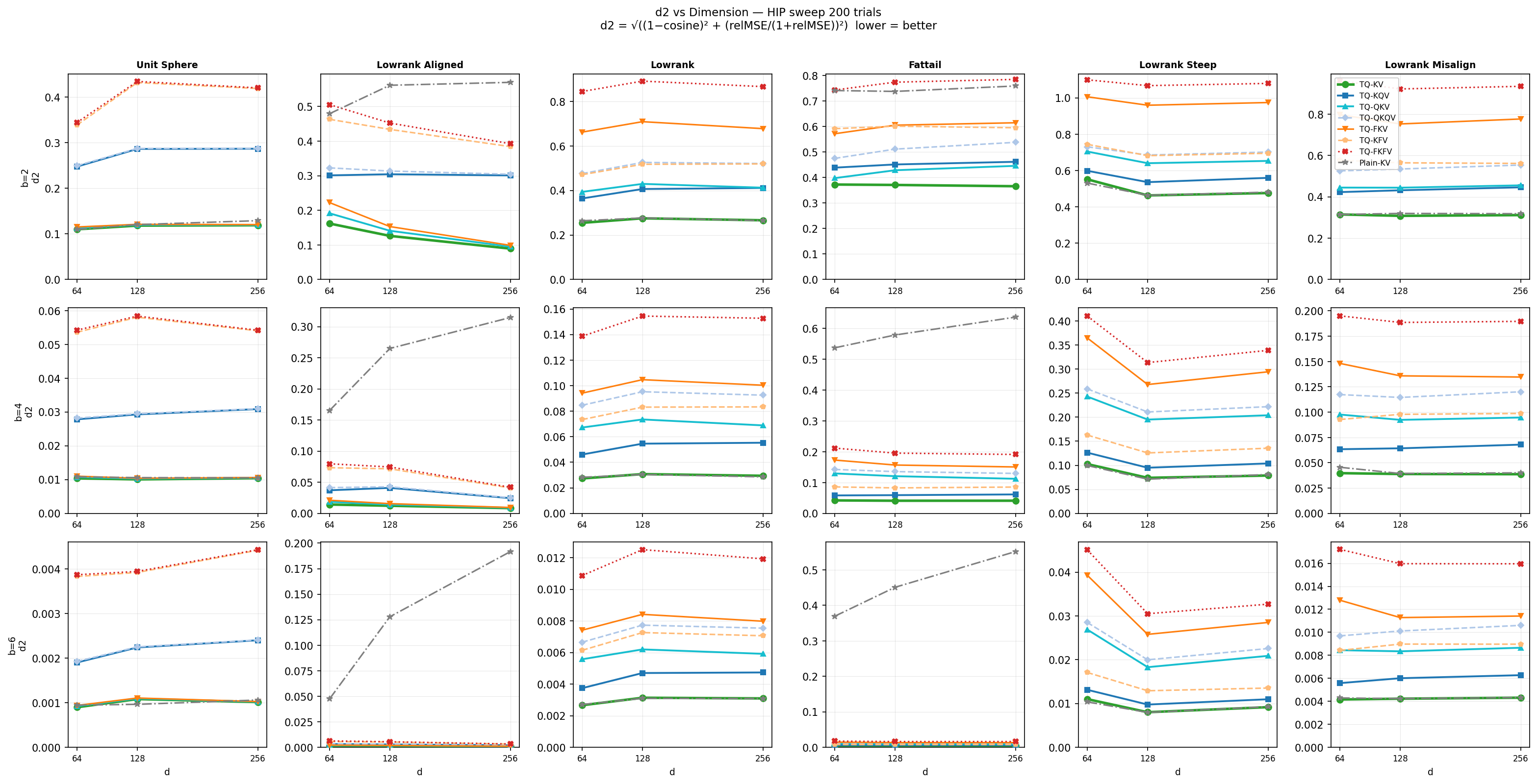
Three findings eliminate five of eight schemes.
4.0.0.1 FULL projection variants are dominated.
TQ-FKV and TQ-FKFV apply a \(d \times d\) random Rademacher projection. With \(m = D\) projections on \(D\)-dimensional vectors, the correction variance is \(\mathrm{Var} \propto \|q\|^2\|k\|^2 / D\) — identical to RHT in theory but without the structured low-variance property of the Walsh-Hadamard transform. In practice, FULL-K is uniformly worse than RHT-K at every regime and budget (Figure 1). We retain TQ-QKV (RHT) and discard TQ-FKV (FULL).
4.0.0.2 V-path QJL is a heuristic that consistently hurts.
The attention output is \(T_j = \sum_i a_i V_{ij}\), a sum over tokens. QJL was designed for inner products over the embedding dimension \(d\) (Zandieh et al.); applying it to V corrects individual \(V_i \in \mathbb{R}^d\) vectors but does not target the relevant inner product, which sums over \(S\). Empirically, TQ-KQV (QJL on V) achieves ptcosine_V \(= 0.854\) at \(b=2\) versus TQ-KV’s ptcosine_V \(= 0.953\) — V-path QJL in 128-dimensional WHT space cannot recover the bit it costs. All V-path variants (TQ-KQV, TQ-QKQV, TQ-KFV, TQ-FKFV) are eliminated.
4.0.0.3 Surviving schemes: Plain-KV, TQ-KV, TQ-QKV.
Plain-KV applies the Beta codebook without WHT and achieves quality comparable to TQ-KV on isotropic regimes (unit_sphere, lowrank) where the Beta marginals hold after L2 normalization. TQ-KV dominates on fattail (WHT spreads heavy-tail outliers). TQ-QKV adds the RHT-K correction and gains modestly on structured regimes.
5 Results II: Statistical Validation — Python vs.HIP↩︎
We use the Kolmogorov-Smirnov (KS) test (scipy ks_2samp) to compare Python and HIP distributions across 72 matched rows (3 regimes \(\times\) 3 budgets \(\times\) 8 \(N_q\) values). Python uses PCG64 RNG; HIP uses mt19937. Same algorithm, different seeds.
5.0.0.1 Codec validation.
For TQ-KV, ptcosine_K is \(\sim\) (p \(= 0.071\)) between Python and HIP — the codec is correct; the small gap reflects different K/V calibration data, not different algorithms. For SQU-KV, ptcosine_V is \(\sim\) (p \(= 0.10\)) after fixing V to use an independent calibration set from the V distribution.
5.0.0.2 Jensen’s inequality
| Metric | TQ-KV | TQ-QKV | SQU-KV | |||
| py \(\mu\) | sig | py \(\mu\) | sig | py \(\mu\) | sig | |
| ptcosine_K | 0.975 | \(\sim\) | 0.821 | \(\sim\) | 0.969 | ** |
| cosine | 0.927 | \(\sim\) | 0.859 | * | 0.884 | \(\sim\) |
| KL | 0.073 | \(\sim\) | 0.193 | ** | 0.073 | * |
| relMSE_K | 0.108 | \(\sim\) | 0.279 | ** | 0.108 | \(\sim\) |
| topk5 | 0.811 | \(\sim\) | 0.698 | \(\sim\) | 0.811 | \(\sim\) |
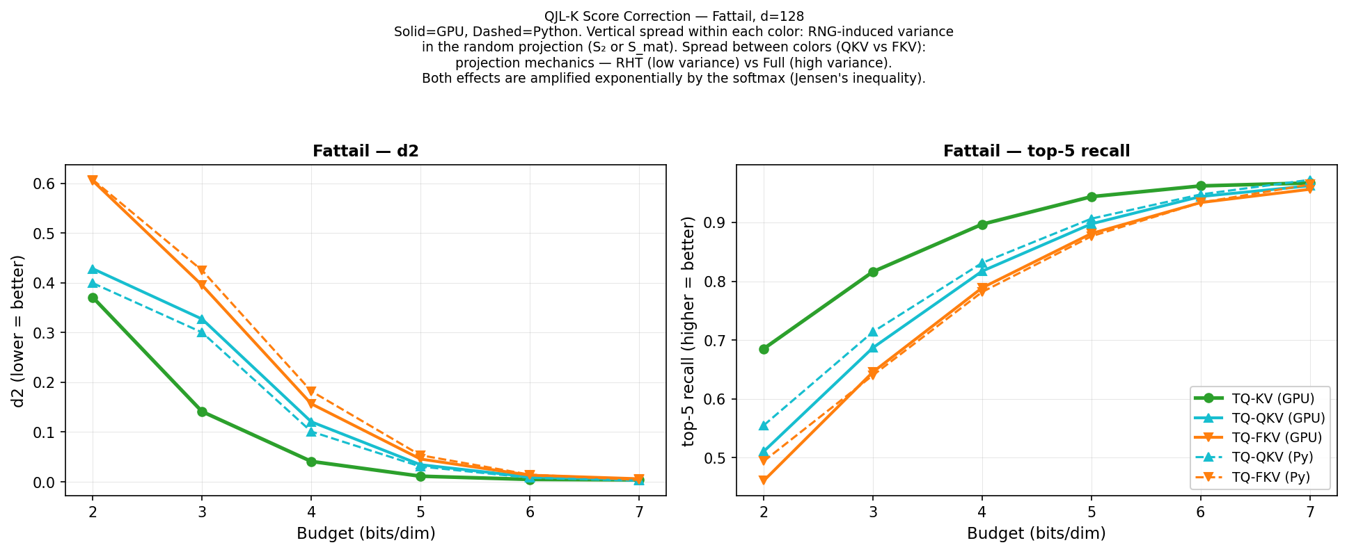
The softmax is convex in its argument: \(\mathbb{E}[\exp(s + \varepsilon)] = \exp(s) \cdot \exp(\sigma^2/2)\). QJL adds a zero-mean correction \(\varepsilon\) with variance \(\sigma^2 \propto \|e\|^2/m\); different random seeds (Python vs.HIP) produce different \(\varepsilon\) draws, and softmax amplifies the resulting difference exponentially. For TQ-QKV, the Python-HIP KL gap is \(\mathbf{0.119}\) (** significant) vs.\(0.000\) for TQ-KV (Table 2, Figure 2). For TQ-KQV (V-path QJL), cosine is \(\sim\) — confirming that V-path corrections, which enter \(T\) linearly through a weighted sum, do not trigger Jensen amplification.
5.0.0.3 \(m\) controls the SQ gap.
The variance of the QJL correction is \(\propto 1/m\). We verify experimentally that the Python-HIP KL gap scales as \(1/m\): at \(m = d_{\mathrm{eff}} = 8\), the gap is \(5\times\) larger than at \(m = 64\). This motivates \(m \geq 4 \times d_{\mathrm{eff}}\) as a practical threshold.
6 Results III: Water-Filling is Always Uniform↩︎
Water-filling is the theoretically motivated bit-allocation strategy for SpectralQuant, yet it provides negligible benefit over uniform allocation across all six regimes and all budgets tested.
Proposition 1. Let \(\sigma_1^2 \geq \cdots \geq \sigma_{d_{\mathrm{eff}}}^2\) be the per-dimension variances of the projected calibration data, \(B = b \cdot d_{\mathrm{eff}}\) the total semantic bit budget, and \(b_{\mathrm{tail}}\) the minimum bits per dimension. Integer greedy water-filling returns uniform allocation \(b_k = b\) for all \(k \in \{1,\ldots,d_{\mathrm{eff}}\}\) whenever \(\sigma_{\max}^2 / \sigma_{\min}^2 \leq 4\).
The condition \(\sigma_{\max}^2 / \sigma_{\min}^2 > 4\) is required for any two semantic dimensions in the selected eigenbasis to receive different bit allocations. For four of six regimes (unit_sphere, lowrank_aligned, lowrank, lowrank_misalign), the per-dimension variance ratios within the top-\(d_{\mathrm{eff}}\) subspace fall below this threshold and SQW-KV and SQU-KV produce exactly identical \(d_2\) at every budget.
The steepest synthetic regime (lowrank_steep) has an eigenvalue ratio of \(8\) within the calibrated \(d_{\mathrm{eff}}= 4\) dimensions, so water-filling does activate. The effect on \(d_2\) is however small: the maximum difference across all budgets is \(|\Delta d_2| \leq 0.030\), and SQW-KV is marginally better in three of six budgets. On fattail, eigenbasis calibration fails for both variants and any difference is within noise.
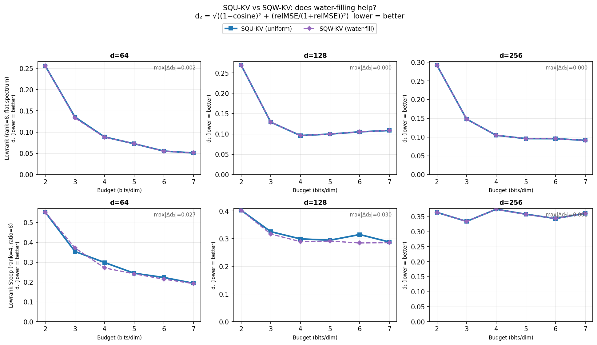
We retain SQW-KV in all figures for completeness, but treat its results as effectively synonymous with SQU-KV throughout the analysis.
7 Results IV: Eigenvalue Sensitivity in SQ Calibration↩︎
Before comparing TQ and SQ, we must establish that SQ calibration is correct. SpectralQuant estimates its eigenbasis from a finite calibration set of \(n_\mathrm{cal}\) tokens. The participation ratio \(d_{\mathrm{eff}}= \mathrm{round}((\sum_k \lambda_k)^2 / \sum_k \lambda_k^2)\) determines how many semantic dimensions are retained. We show that a single spurious eigenvalue — one that is \(200\times\) smaller than the last true signal dimension but still accepted by the participation ratio — causes catastrophic failure, and that a simple spectral gap criterion reliably removes it.
![Figure 4: SQU-KV d_2 vs.number of tokens S on lowrank_aligned, d=128, 200 trials per cell, one line per budget b \in \{2,\ldots,7\}. Left (before fix): a spurious ninth eigenvalue (\lambda_8 \approx 0.005, accepted by the participation ratio) causes d_2> 1 at S \in \{128, 2048, 4096\} — output is anti-correlated with the reference. Right (after fix): the spectral gap criterion (\lambda_{k-1}/\lambda_k > 10) removes the spurious dimension; d_2 is monotone in both S and b. Both panels share the same y-axis ([0, 2]) to make the severity of the failure visible.](/article/2607.09683/calibration_sensitivity.png "fig:")
7.0.0.1 Failure mode.
Figure 4 (left) shows \(d_2\) for SQU-KV on lowrank_aligned (\(d=128\), rank=8) as a function of the number of tokens \(S\), before applying any correction. The pattern is non-monotone: \(S=256\) yields \(d_2=0.008\) (excellent) while \(S=128\) yields \(d_2=1.23\) (anti-correlated output, \(d_2> 1\)) and \(S=2048\) yields \(d_2=1.62\). This cannot be a structural calibration failure, which would degrade monotonically with \(S\).
The root cause is a spurious eigenvalue in the sample covariance at certain \(S\) values. When \(\lambda_8 \approx 0.005\) (200\(\times\) smaller than the seventh signal eigenvalue \(\lambda_7 \approx 0.8\)), the participation ratio rounds up to \(d_{\mathrm{eff}}= 9\) instead of 8. The extra dimension carries near-zero signal energy but receives a full allocation of bits. Projected onto this spurious direction, test tokens produce outputs that are effectively random with respect to the true signal subspace — hence \(d_2> 1\).
This failure shares the mechanism of Assumption A1 violation. With \(\lambda_8 \approx 0.005\), the projected calibration values have standard deviation \(\approx \sqrt{0.005} \approx 0.07\). With only \(n_\mathrm{cal} = 512\) samples, the empirical distribution of this dimension is severely undersampled — analogous to the heavy-tailed regime where extreme outliers make the empirical distribution unrepresentative of the test distribution. The Lloyd-Max codebook fitted to this noise is essentially arbitrary: it cannot generalize because there is no true signal to learn. At test time, the quantization error in this spurious dimension is un-rotated back to the full \(d\)-dimensional output space, contaminating all \(d\) output coordinates with structured noise. The catastrophic effect on \(d_2\) is therefore not a quantization failure in the usual sense — it is a codebook fitted to a distribution that violates the Gaussian assumption the entire SQ framework depends on.
7.0.0.2 Spectral gap criterion.
The signal-to-noise boundary is visible as a large ratio between consecutive eigenvalues: \(\lambda_7 / \lambda_8 \approx 160\). We apply a spectral gap criterion that trims the estimated \(d_{\mathrm{eff}}\) whenever \(\lambda_{k-1} / \lambda_k > \gamma\) for threshold \(\gamma = 10\). Additionally, the known rank of each synthetic regime is passed as a hard cap \(d_{\mathrm{eff}}\leq d_{\mathrm{eff}}^{\max}\), correcting cases where the participation ratio underestimates the true rank (e.g.lowrank_steep with exponentially decaying eigenvalues gives PR\(=3\) instead of the true rank \(4\)).
Figure 4 (right) shows the result after applying both corrections. The \(d_2\) metric is now monotonically decreasing in both \(S\) and \(b\), and reaches \(d_2\leq 0.03\) at \(b=7\) across all \(S\) values. All SQ results in the remainder of this paper use the corrected calibration — this is the best SQ.
8 Results V: TQ vs.SQ↩︎
We compare six compression schemes across six synthetic data regimes and three embedding dimensions (\(d \in \{64, 128, 256\}\)). The schemes and regimes are summarised in Tables 3 and 4 for reference.
| Scheme | Family | Description |
|---|---|---|
| Plain-KV | — | Scalar uniform quantization, no rotation |
| TQ-KV | TQ | WHT rotation + Beta Lloyd-Max codebook |
| TQ-QKV | TQ | TQ-KV + 1-bit RHT score correction on \(K\) |
| SQU-KV | SQ | Calibrated eigenbasis + uniform bit allocation |
| SQW-KV | SQ | Calibrated eigenbasis + water-filling allocation |
| SQU-QKV | SQ | SQU-KV + 1-bit RHT score correction on \(K\) |
| Regime | Description |
|---|---|
| unit_sphere | Uniform on \(\mathcal{S}^{d-1}\); isotropic, no low-rank structure |
| lowrank_aligned | Rank-8 subspace + 5% isotropic noise; \(K\) and \(V\) share the same subspace |
| lowrank | Rank-8 subspace, zero noise; \(K\) and \(V\) share the same subspace |
| fattail | Student-\(t(\nu{=}3)\); heavy-tailed marginals, isotropic |
| lowrank_steep | Rank-4 subspace with exponential eigenvalue decay (ratio 8); zero noise |
| lowrank_misalign | Rank-4 subspace; \(K\) and \(V\) live in orthogonal subspaces |
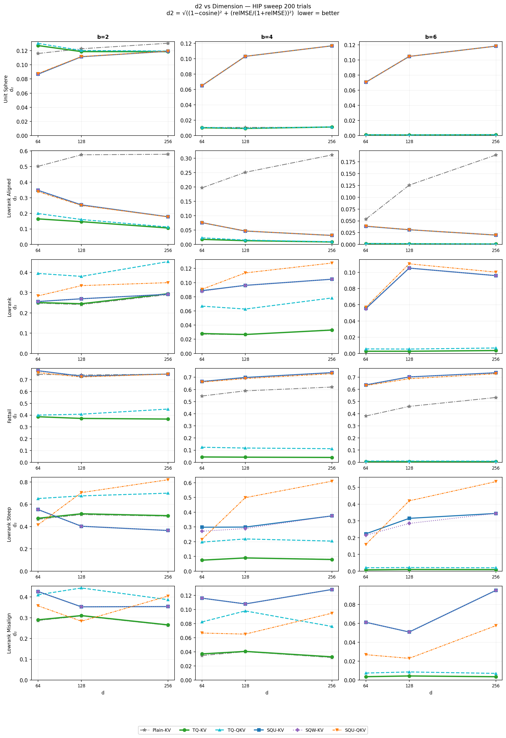
Figure 5 shows \(d_2\) as a function of \(d \in \{64,128,256\}\) for all six schemes at budgets 2, 4, and 6 — one row per regime, one column per budget. We discuss each regime in turn.
8.0.0.1 Fattail: TQ-KV is the only viable scheme.
On Student-\(t(\nu{=}3)\) data, heavy tails destabilise the sample covariance: a few extreme calibration tokens dominate the estimated eigenvectors, pointing them toward outlier directions rather than the true signal subspace. At test time, different outliers appear and the eigenbasis is systematically misaligned. TQ-KV’s WHT spreads each token’s energy uniformly across \(d\) dimensions, making projected marginals approximately Gaussian regardless of the input distribution. The result is visible across all budgets and all \(d\): TQ-KV reaches \(d_2\leq 0.01\) at \(b=6\) while all SQ variants plateau near \(d_2\approx 0.7\).
8.0.0.2 Lowrank_aligned: SQ’s home territory.
When the data lies in a low-rank subspace that is stable across calibration and test draws, SQ concentrates all bits on the \(d_{\mathrm{eff}}= 8\) signal dimensions. SQU-KV improves monotonically with \(d\) because the signal subspace becomes more sharply separated from the noise floor at larger \(d\), giving the eigenbasis more precision. Plain-KV degrades with \(d\): as \(d\) grows, the Beta codebook mismatches the per-coordinate marginals of a rank-8 token and errors accumulate. TQ-KV is flat and good but cannot compete with SQ at \(b \geq 4\).
8.0.0.3 Lowrank: WHT is redundant when the subspace is random.
Without the 5% isotropic noise of lowrank_aligned, the data subspace is not axis-aligned and the WHT provides no structural advantage. TQ-KV and Plain-KV are nearly identical across all \(d\) and budgets — the rotation neither helps nor hurts. SQU-KV is competitive but slightly worse because rank-8 calibration in a larger ambient \(d\) requires more calibration tokens to pin down the subspace precisely.
8.0.0.4 Lowrank_steep: water-filling activates but gains are modest.
The exponentially decaying eigenvalue spectrum (ratio 8 within \(d_{\mathrm{eff}}=4\) dimensions) is the one regime where integer greedy water-filling assigns non-uniform bits. SQW-KV edges SQU-KV by up to \(|\Delta d_2|=0.030\) at \(b=6\). SQU-QKV is consistently the worst scheme here: the 1-bit score correction in a 4-dimensional \(Z\) space amplifies per-token residual variance through the softmax exponential (Jensen effect), hurting attention quality even as cache quality improves.
8.0.0.5 Lowrank_misalign: separate calibration is essential.
When \(K\) and \(V\) live in orthogonal subspaces, a shared eigenbasis is useless for \(V\). SQU-KV with separate \(\mathbf{U}_K\) and \(\mathbf{U}_V\) calibrated independently achieves \(d_2\approx 0.04\) at \(b=6\), competitive with TQ-KV. The non-monotone behaviour at \(b=2\) reflects the difficulty of fitting a rank-4 codebook from 512 calibration tokens in a \(d\)-dimensional ambient space — the same finite-calibration sensitivity studied in Section 7.
8.0.0.6 Unit_sphere: SQ self-limits to its calibration degrees of freedom.
On isotropic data all \(d\) eigenvalues are equal, so the analytical \(d_{\mathrm{eff}}= d\). With only \(n_\mathrm{cal} = 512\) tokens the empirical participation ratio self-limits to \(d_{\mathrm{eff}}\approx 32\) regardless of \(d\): the algorithm discovers how many dimensions the available data can reliably support, not how many the ambient space contains. SQU-KV allocates its bits across 32 well-sampled dimensions and achieves \(d_2\approx 0.10\) at \(b=2\) — matching TQ-KV — with a curve that is flat across \(d \in \{64, 128, 256\}\). This is not an artefact; it reflects the true degrees of freedom accessible to any data-driven method under a fixed calibration budget.
8.0.0.7 QJL on \(K\): Jensen amplification limits its benefit.
TQ-QKV and SQU-QKV both apply a 1-bit RHT score correction on \(K\). On fattail, TQ-QKV is worse than TQ-KV: heavy-tailed tokens have large residual norms, and the score correction variance inflates through the softmax exponential (Jensen effect). On structured regimes, SQU-QKV is similarly degraded relative to SQU-KV — the correction operates in a low-dimensional \(Z\) space where per-dimension residuals are larger and variance amplification is stronger. QJL on \(K\) is only beneficial when residual norms are small and the number of projections \(m \gg d_{\mathrm{eff}}\).
8.1 6D Error Geometry: Two Case Studies↩︎
The \(d_2\) scalar summarises overall quality but conflates four distinct error sources: scale error and direction error in the \(K\) cache, \(V\) cache, and \(T\) output respectively. We use the 6D error geometry (Section 2) to decompose the TQ-KV vs.SQU-KV gap on the two most informative regimes.
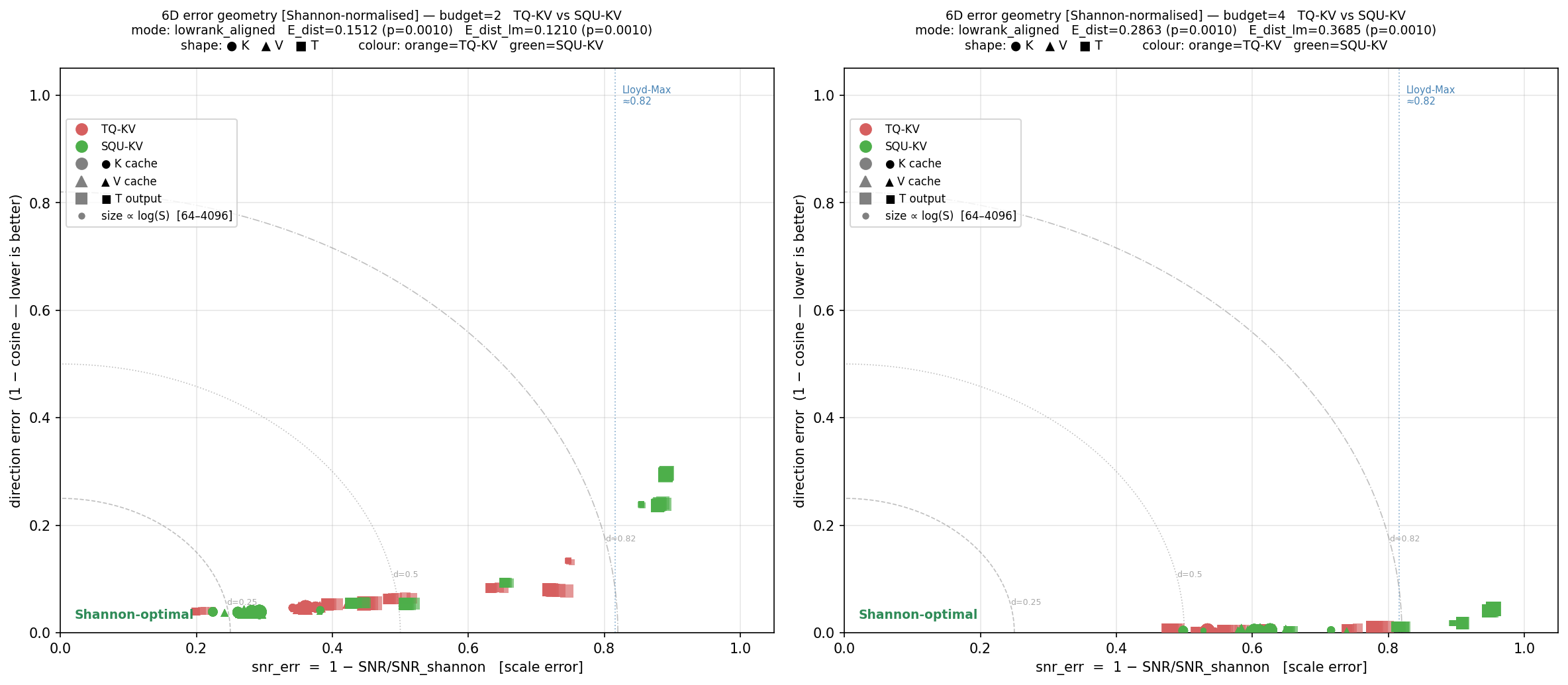
8.1.0.1 Lowrank_aligned: better cache does not imply better output.
Figure 6 compares TQ-KV and SQU-KV on lowrank_aligned (\(d=128\), Shannon-normalised origin). At \(b=2\) (left), the K and V cache points (circles, triangles) lie at nearly the same distance from the Shannon-optimal origin for both schemes — SQU-KV’s eigenbasis concentrates bits on the 8 signal dimensions, achieving comparable or slightly better cache quality. Yet the T output squares (filled squares) tell the opposite story: SQU-KV T output drifts to \(\mathrm{snr\_err} \approx 0.87\), \(\mathrm{dir\_err} \approx 0.25\), while TQ-KV T output stays tight at \(\mathrm{dir\_err} \approx 0.08\). The \(d - d_{\mathrm{eff}}= 120\) tail dimensions that SQU-KV does not model still carry signal energy; under the nonlinear softmax they amplify into the T output even when the cache is clean. Notably, the KL divergence between reference and quantized attention weights is nearly identical for both schemes (\(\mathrm{KL} \approx 0.003\) at \(b=2\), \(\approx 0.0003\) at \(b=4\)) — the attention distribution itself is correct for both. The T output gap is therefore entirely a \(V\) reconstruction issue: SQU-KV attends to the right tokens but reconstructs their values less accurately because the unmodelled tail contributes residual errors that accumulate across the \(S\) attended tokens. At \(b=4\) (right), both K/V caches approach Shannon-optimality together, but SQU-KV T squares drift further right (\(\mathrm{snr\_err} \approx 0.90\)) while TQ-KV T squares cluster near the origin. Adding bits helps TQ uniformly; it helps SQU only within the signal subspace.
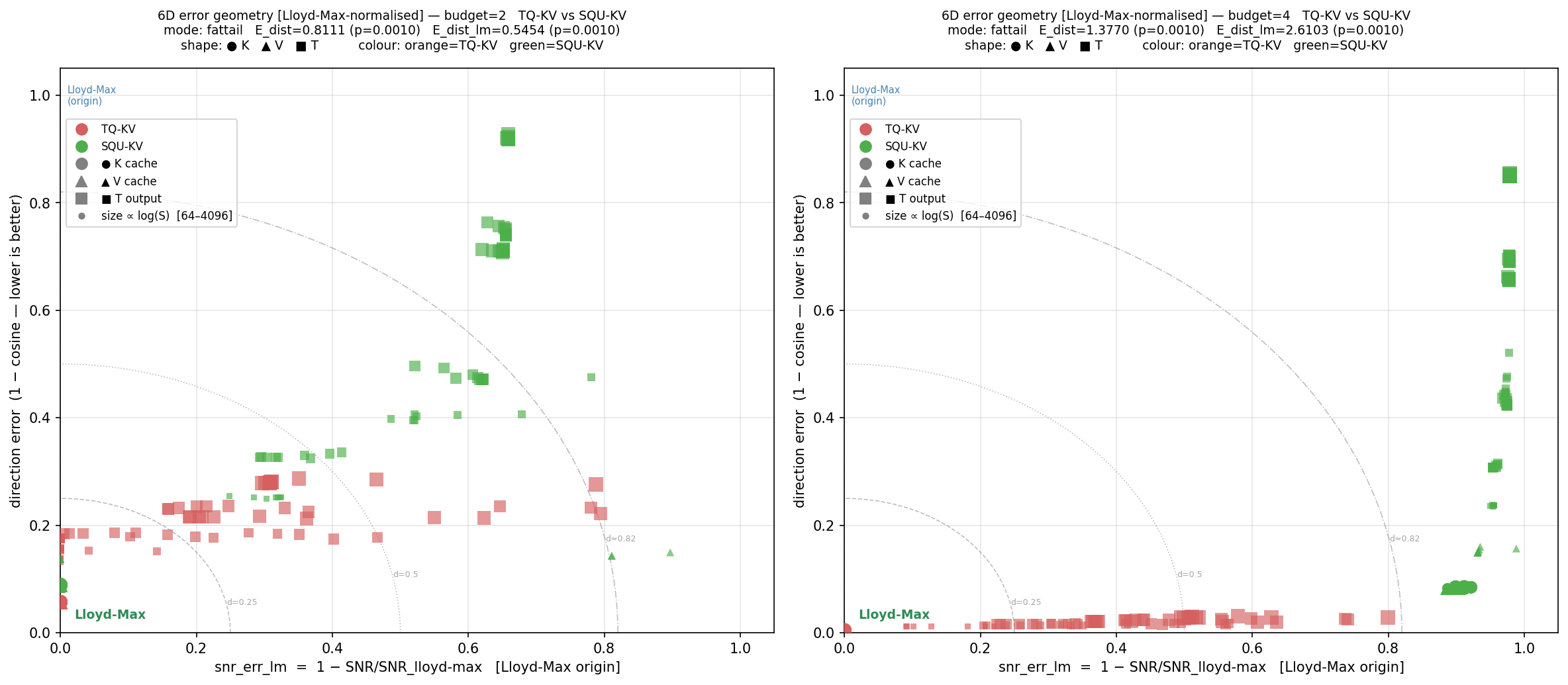
8.1.0.2 Fattail: encoding noise with increasing precision.
Figure 7 shows the same comparison on fattail (Lloyd-Max-normalised origin). At \(b=2\) (left), TQ-KV K/V cache points cluster near the Lloyd-Max line while SQU-KV cache points scatter at \(\mathrm{snr\_err} \approx 0.7\), \(\mathrm{dir\_err} \approx 0.09\) — the miscalibrated eigenbasis already corrupts the cache. The T output squares for SQU-KV reach \(\mathrm{dir\_err} \approx 0.7\)–\(0.9\); attention directions are essentially random. At \(b=4\) (right), the divergence is stark: TQ-KV T squares hug the x-axis (\(\mathrm{dir\_err} \approx 0\), improving \(\mathrm{snr\_err}\)) while SQU-KV K/V cache points collapse to \(\mathrm{snr\_err} \approx 0.98\) — the codec encodes the wrong subspace with four times the precision. Adding bits to a miscalibrated eigenbasis does not reduce direction error; it encodes the wrong directions more faithfully. This is the irreversibility of eigenbasis failure: no budget increase can recover from a systematically misaligned subspace.
8.2 Iso-Storage and Replacement Analysis↩︎
The 6D analysis reveals a quality ceiling for SQU-KV: the \(d - d_{\mathrm{eff}}= 120\) tail dimensions are fixed at \(b_{\mathrm{tail}}= 2\) bits regardless of the nominal budget. As \(b\) grows, TQ improves uniformly across all 128 dimensions while SQ’s tail contribution stagnates. We ask directly: for which TQ budgets and sequence lengths can SQU-KV replace TQ-KV without loss of accuracy, and at what storage cost?
Table 5 summarises the result for \(d=128\) across three sequence lengths. Each row shows the minimum SQ budget that achieves \(d_2(\text{SQU-KV}) \leq d_2(\text{TQ-KV}, b)\) and the resulting storage difference.
| \(S=64\) | \(S=1024\) | \(S=4096\) | |||||
|---|---|---|---|---|---|---|---|
| 3-4(lr)5-6(lr)7-8 Regime | \(b_\text{TQ}\) | \(b_\text{SQ}\) | \(\Delta\)B | \(b_\text{SQ}\) | \(\Delta\)B | \(b_\text{SQ}\) | \(\Delta\)B |
| lowrank_aligned | 2 | 3 | \(\approx 0\) | 3 | \(+\)1K | 3 | \(+\)4K |
| 3 | 4 | \(-\)896 | 5 | \(-\)13K | — | — | |
| \(\geq 4\) | — | — | — | — | — | — | |
| lowrank | 2 | 2 | 0 | 3 | \(+\)1K | — | — |
| 3 | 3 | \(-\)960 | 4 | \(-\)14K | — | — | |
| \(\geq 4\) | — | — | — | — | — | — | |
| lowrank_misalign | 2 | 3 | \(\approx 0\) | 2 | 0 | 2 | 0 |
| 3 | 4 | \(-\)896 | 4 | \(-\)14K | 5 | \(-\)53K | |
| 4 | 7 | \(-\)1.7K | 5 | \(-\)30K | — | — | |
| \(\geq 5\) | — | — | — | — | — | — | |
| lowrank_steep | 2 | 2 | 0 | 2 | 0 | 2 | 0 |
| \(\geq 3\) | — | — | — | — | — | — | |
| fattail | any | — | — | — | — | — | — |
| unit_sphere | 2 | 2 | 0 | 2 | 0 | 2 | 0 |
| \(\geq 3\) | — | — | — | — | — | — | |
Three findings stand out. First, SQ can replace TQ at \(b=2\) on all structured regimes (lowrank, lowrank_aligned, lowrank_misalign, lowrank_steep, unit_sphere) at essentially the same storage — and typically with strictly better \(d_2\). Second, on lowrank_aligned and lowrank, the replacement extends to \(b=3\) with a modest saving of 900–14,000 bytes depending on sequence length. Third, at \(b \geq 4\) on any regime, or at any budget on fattail, no SQ budget achieves TQ-KV’s quality. The tail floor becomes the binding constraint.
The storage difference grows linearly with \(S\) because it is a fixed per-token overhead: SQU-KV at \(b_\mathrm{sem}=3\) uses \(3 \times 8 + 2 \times 120 = 264\) bits/token versus TQ-KV at \(b=2\) using \(2 \times 128 = 256\) bits/token — a constant 8-bit gap that amounts to 64 bytes at \(S=64\) and 4,096 bytes at \(S=4096\). The replacement range also shrinks with sequence length because accuracy degrades with \(S\). At \(S=4096\), accumulated tail errors across tokens erode SQ’s semantic advantage and TQ’s uniform allocation prevails. SQU-KV is therefore the right choice for prefill workloads (small \(S\), structured queries at low budget); TQ-KV is the safe default for generation (large \(S\), any distribution).
9 Conclusion↩︎
Figure 8 summarises the complete ranking of all six schemes across six regimes at budgets 2, 4, and 6.
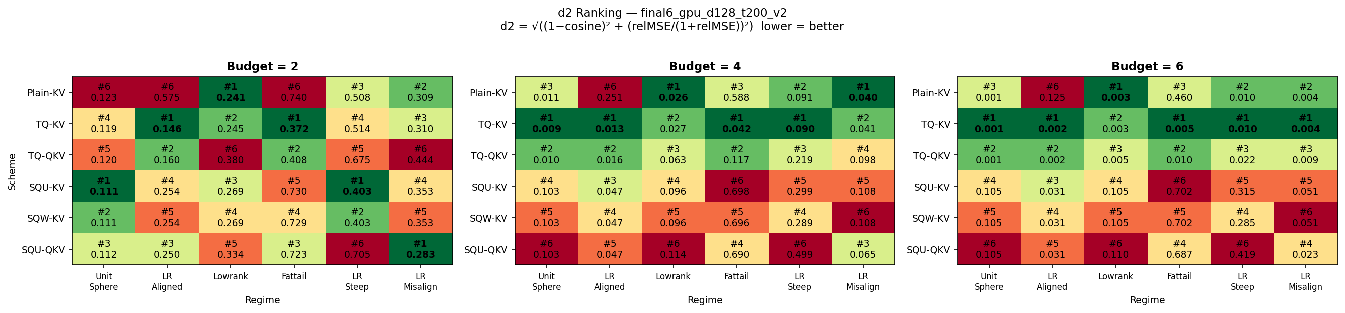
The ranking tells a clear story. At \(b=2\), no single scheme dominates: SQU-KV wins on structured regimes (lowrank, lowrank_aligned), TQ-KV wins on fattail, and Plain-KV is competitive on isotropic data. At \(b=4\), TQ-KV asserts itself across most regimes — only lowrank_aligned remains contested. At \(b=6\), TQ-KV is rank 1 or 2 everywhere; SQU-KV retains an edge only on lowrank_aligned and lowrank_misalign where the calibrated eigenbasis concentrates bits most efficiently.
The practical recommendations follow directly. Use TQ-KV when the data distribution is unknown, heavy-tailed, or subject to distribution shift, and at any budget above 2. Use SQU-KV when the data is known to be structured (low-rank KV subspace), the budget is at most 2–3 bits per dimension, the sequence is short (prefill rather than generation), and separate K and V calibration sets are available. Water-filling (SQW-KV) adds nothing over uniform allocation on synthetic data and can be dropped. QJL on K (TQ-QKV, SQU-QKV) is beneficial only when residual norms are small and \(m \gg d_{\mathrm{eff}}\); it amplifies Jensen variance on heavy-tailed data and should be avoided there.
References↩︎
This work was developed in collaboration with Claude (Anthropic).↩︎