1 Introduction↩︎

Recent research demonstrates that rm codes [1] achieve channel capacity under a wide range of channels, such as the binary erasure channel [2], the bsc [3], [4], and the bms channel [5]–[8]. In addition to the capacity-achieving capability, the rm codes are structurally similar to polar codes [9] and also exhibit a polarization effect [10].

Decoding with affordable complexity for rm codes is the key to utilizing the desired characteristic mentioned. The first decoding algorithm for rm codes is majority-vote decoding [11] that can correct error patterns with a weight of fewer than half of the minimum distance of rm codes. For order \(r=1\) rm codes, ml decoding performance can be achieved under a complexity \(O\left(n\log_{2}\left(n\right)\right)\) using the fht decoding [12], [13], where \(n\) is the code length. Many decoding algorithms are proposed for rm codes with \(r\geq2\). For example, Dumer’s recursive list decoding can achieve ml decoding performance given a sufficiently large list size [14].

The recently proposed rpa decoding and its list decoding are observed to achieve near-ml decoding performance for a range of code lengths and code rates [15]. Given its near-ml decoding performance, theoretical analysis on rpa decoding is conducted in the literature [16]–[18]. It is proven in [16] that the rpa decoding can asymptotically achieve vanishing probability over the bsc for rm codes with \(r\leq\log\left(cm\right)\), where \(m\) is the code length parameter and \(c\) is a constant that is proportional to the cross-over probability of the bsc. Later, the result is extended to the bms channel [17].

A variant of rpa decoding, namely cpa decoding, is proposed to reduce the computational complexity of rpa decoding by removing repeated subspaces [19]. cpa decoding targets the soft-decision variant of rpa decoding and, as pointed out in [19], it is closely related to bp decoding. The similarity of the decoding results under different subspaces in cpa decoding is first analyzed in [20]. The error patterns encountered during rpa and cpa decoding are analyzed in [18], where it is further shown that rpa and cpa decoding with \(2t+1\) subspaces can correct up to \(t\) errors. Moreover, a recent work shows that the pa decoding (rpa decoding and its variants) can decode error patterns with a weight of fewer than half the minimum distance efficiently [21]. Also, cpa decoding is further simplified in [22], where the extrinsic inter-iteration update is replaced by the broadcast inter-iteration update.

Theoretical research [16]–[18], [21] on rpa and cpa decoding focuses on hard-decision decoding, where the number of errors encountered by decoding algorithms is investigated, and analysis tools for soft-decision decoding, which handle the probability density function of received soft information, are still missing in the literature. In this work, we analyze soft-decision cpa decoding, propose a density evolution model to track changes in the density function of soft-decision outputs from cpa decoding, and perform an asymptotic analysis using the proposed density evolution model. The following contributions on soft-decision cpa decoding are made:

1. We found that cpa decoding returns the exact marginal probability. Also, we prove that cpa decoding is symmetric with respect to the transmitted codeword.

2. We propose density evolution to analyze the density function of the soft-decision output from each iteration of cpa decoding over the biawgn channel. Proposed density evolution captures the fast reduction in the mean and variance of the soft information returned from cpa decoding, which qualitatively explains the decoding mechanism and the fast convergence of cpa decoding.

3. Based on the proposed density evolution, we perform an asymptotic analysis and find that the soft-decision cpa decoding achieves vanishing error probability when the rm code has a vanishing code rate.

This work is structured as follows. Section 2 shows the necessary background of cpa decoding. Section 3 presents key properties that facilitate the condition for applying the density evolution. Section 4 presents the density evolution model for the cpa decoding. Section 5 is the asymptotic analysis of cpa decoding based on our proposed density evolution model. Section 6 concludes this work.

2 Preliminaries↩︎

2.1 Notations↩︎

Matrices and vectors are denoted as bold upper-case letters (\(\boldsymbol{M}\)) and bold lower-case letters (\(\boldsymbol{v}\)), respectively. The transpose operation is \(^\top\), and a projection based on the coset of a subspace \(\mathbb{B}_{i}\) is denoted by the subscript \(/\mathbb{B}_{i}\). Binary indices are denoted by the letter \(z\). The probability of an event is denoted by \(\mathbb{P}\left(\cdot\right)\). The probability density function is denoted by \(\mathrm{p}\left(\cdot\right)\).

2.2 RM Codes↩︎

rm\(\left(m,r\right)\) codes are \(\left(n,k\right)\) linear codes, where \(n=2^{m}\) is the code length, \(k=\sum_{i=0}^{i=r}\binom{m}{i}\) is the code dimension, \(0 \leq r \leq m\), and the code rate equals \(R=\tfrac{k}{n}\). The generator matrix for encoding the rm\(\left(m,r\right)\) codes can be constructed in the following two steps:

1. The generator matrix for the RM\((m,m)\) code (\(\boldsymbol{G}(m,m)\)) is obtained by applying the \(m\)-th Kronecker power of the base matrix \(\boldsymbol{F}\) [9]: \[\boldsymbol{G}(m,m)=\boldsymbol{F}^{\otimes m}, \text{ }\boldsymbol{F}= \begin{bmatrix} 1&0\\ 1&1 \end{bmatrix}\text{.}\]

2. Select rows with the \(k\) largest Hamming weights, which are at least \(2^{m-r}\), in \(\boldsymbol{G}\left(m,m\right)\) to compose the generator matrix \(\boldsymbol{G}\left(m,r\right)\) for the rm\(\left(m,r\right)\) code.

The dual code of the rm\(\left(m,r\right)\) code is the rm\(\left(m,m-r-1\right)\) code, so the parity-check matrix \(\boldsymbol{H}\) of the RM\((m,r)\) code is \(\boldsymbol{H}=\boldsymbol{G}(m,m-r-1)\) [23]. Valid codewords \(\boldsymbol{c}\in \text{RM}(m,r)\) produce an all-zeros syndrome vector \(\boldsymbol{s}=\boldsymbol{H}\boldsymbol{c}^{\top}=\boldsymbol{0}\).

2.3 Collapsed Projection-Aggregation Decoding↩︎

cpa decoding is a three-step iterative decoding algorithm, namely:

1. Projection: In this step, the received llr vector \(\boldsymbol{l}\) of the rm\(\left(m,r\right)\) code is used to compute the llr of the rm\(\left(m-r+1,1\right)\) codes by projecting to the \(\left(r-1\right)\)-dimensional subspace \(\mathbb{B}_{i}\) \[\begin{align} \boldsymbol{l}_{/\mathbb{B}_{i}}(T) &=2\tanh^{-1}\left(\underset{z\in T}{\prod}\tanh\left(\frac{\boldsymbol{l}(z)}{2}\right)\right)\text{,}\\ \end{align} \label{eqn:cpallrproj}\tag{1}\] where \(T\) is the coset of the subspace \(\mathbb{B}_{i}\) of dimensions \(r-1\). It is shown in [24] that the \(\left(r-1\right)\)-dimensional subspaces can be decomposed into \(r-1\) \(1\)-dimensional subspaces: \[\begin{align} &h_{2^{r-1}}(l_{1},l_{2},...,l_{2^{r-1}})\\ &= 2\tanh^{-1}\left(\prod_{i=1}^{2^{r-1}}\tanh\left(\frac{l_{i}}{2}\right)\right)\\ &= h_{2} (h_{2}(h_{2}...), h_{2}(h_{2}...))\text{,} \end{align} \label{eqn:dimension95decomposition}\tag{2}\] where \(h_{2}\left(A,B\right) = 2\tanh^{-1}\left(\tanh\left(\frac{A}{2}\right)\tanh\left(\frac{B}{2}\right)\right)\) is the projection function for the \(1\)-dimensional subspace, which is also known as the box-plus (\(\boxplus\)) operator [25], and \(l_{i}\in\boldsymbol{l}\). There are \(n_{\mathbb{B}}=\binom{m}{r-1}_{2}\) different \((r-1)\)-dimensional subspaces in cpa decoding.

2. fht decoding: The projected llr vector of rm\(\left(m-r+1,1\right)\) codes is decoded by ml fht decoding, and the decoded codeword is defined as \[\hat{\boldsymbol{y}}_{/\mathbb{B}_{i}} = \mathop{\mathrm{arg\,max}}_{\boldsymbol{c}\in\mathrm{\gls{rm}}\left(m-r+1,1\right)}\mathbb{P}\left(\boldsymbol{l}_{/\mathbb{B}_{i}} \mid \boldsymbol{c}\right)\text{,} \label{eqn:def95ml95fht}\tag{3}\] where \(\boldsymbol{l}_{/\mathbb{B}_{i}}\) is the llr vector after the projection function. The decoded bit \(\hat{\boldsymbol{y}}_{/\mathbb{B}_{i}}\!\left(T\right)\) estimates the parity check of received code bits in the same coset \(T\).

3. Aggregation: Given the received llr vector and the decoding result from the fht decoding, new llrs of the received code bits are computed by \[\begin{align} &\hat{\boldsymbol{l}}\left(z\right)\\ &=\sum_{i=1}^{n_{B}} (-1)^{\hat{\boldsymbol{y}}_{/\mathbb{B}_{i}}(T)}\\ &\left(2\tanh^{-1}\left(\underset{{z}_{j}\in T \setminus \{z\}}{\prod}\tanh\left(\frac{\boldsymbol{l}(z_{j})}{2}\right)\right)\right)\\ &\stackrel{(a)}{=}\sum_{i=1}^{n_{B}} 2\tanh^{-1}\left( \tanh\left(\frac{+\infty \times (-1)^{\hat{\boldsymbol{y}}_{/\mathbb{B}_{i}}(T)}}{2}\right)\right.\\ &\left.\underset{{z}_{j}\in T \setminus \{z\}}{\prod}\tanh\left(\frac{\boldsymbol{l}({z}_{j})}{2}\right)\right)\text{,} \end{align} \label{eqn:llraggr}\tag{4}\] where the equality \((a)\) in 4 holds according to [24]. The average of the aggregated llr vector (\(\bar{\boldsymbol{l}}=\hat{\boldsymbol{l}}/ n_{\mathbb{B}}\)) is either fed to the next iteration, or hard decisions of \(\bar{\boldsymbol{l}}\) is returned as the decoded codeword if the maximum number (\(N_{\text{max}}\)) of iterations or an early-stopping criterion (e.g., the difference in the L2 norm between soft information returned from two consecutive iterations is smaller than a threshold \(\theta\) [15], [19]) is met.

3 Revisiting cpa Decoding↩︎

Before building the density evolution model, several key properties should be verified so that this analysis tool can be used. For example, the density evolution for ldpc codes is performed under the assumption of an infinite code length [26] because factor graphs of ldpc codes will have a tree structure [27], and the exact marginal probability can be computed by the bp decoding when the factor graph structure is a tree [27].

We first show that the three-step process of cpa decoding resembles the exact marginal probability, and results returned from different subspaces can be viewed as different realizations of the random variable. Also, to simplify the analysis process, we usually assume the all-zeros or all-ones codeword is sent. Hence, we need to show that cpa decoding is symmetric regardless of the transmitted codeword. While the symmetry of the rpa decoding is proved in [15], the proof of the symmetry of cpa decoding is missing in the literature, and we prove the symmetry property of cpa decoding by modifying the proof for the rpa decoding in [15].

3.1 Exact Marginal Probability Computed By cpa Decoding↩︎

In this section, we would like to show that cpa decoding estimates the exact marginal probability, so we do not need to find whether there are cycles present in the Tanner graph structure for cpa decoding [19].

The llr \(\boldsymbol{l}\left(z\right)\) used in the first iteration is defined as \[\boldsymbol{l}\left( z \right) = \ln\left( \frac{\mathbb{P}\left( \mathsf{Y}\left(z\right) = \boldsymbol{y}\left(z\right) \mid \boldsymbol{c}\left(z\right) = 0 \right) }{\mathbb{P}\left( \mathsf{Y}\left(z\right) = \boldsymbol{y}\left(z\right) \mid \boldsymbol{c}\left(z\right) = 1 \right)} \right)\text{,} \label{eqn:def95llr}\tag{5}\] where \(\mathsf{Y}\left(z\right)\) is the output random variable at index \(z\) from the biawgn channel, and \(\boldsymbol{y}\left(z\right)\) is the realization of \(\mathsf{Y}\left(z\right)\). The following proposition shows the meaning behind the projection function.

The meaning of this \(\tanh\left(\cdot\right)\) update rule is also well-investigated in the literature, such as in [25] (i.e., box-plus \(\boxplus\)), and used in theoretical analysis of decoding algorithms [26], [28]. More details regarding this \(\tanh\left(\cdot\right)\) update rule can refer to [25], [28]–[32]. To fit into the context of the pa decoding, we extend the proof in [15] to cpa decoding to support the analysis that will be done in this work.

As shown in 4 , the output \(\hat{\boldsymbol{y}}_{/\mathbb{B}_{i}}\!\left(T\right)\) from the fht decoding can be viewed as having a llr \[\begin{align} &\ln \left( \frac{\mathbb{P}\left(\boldsymbol{l}_{/\mathbb{B}_{i}}\mid \hat{\boldsymbol{y}}_{/\mathbb{B}_{i}},\hat{\boldsymbol{y}}_{/\mathbb{B}_{i}}\!\left(T\right)=0\right)}{\mathbb{P}\left(\boldsymbol{l}_{/\mathbb{B}_{i}}\mid \hat{\boldsymbol{y}}_{/\mathbb{B}_{i}},\hat{\boldsymbol{y}}_{/\mathbb{B}_{i}}\!\left(T\right)=1\right)} \right)\\ &=\ln \left( \frac{\mathbb{P}\left(\boldsymbol{l}_{/\mathbb{B}_{i}},\hat{\boldsymbol{y}}_{/\mathbb{B}_{i}}\mid \hat{\boldsymbol{y}}_{/\mathbb{B}_{i}}\!\left(T\right)=0\right)/\mathbb{P}\left(\hat{\boldsymbol{y}}_{/\mathbb{B}_{i}}\right)}{\mathbb{P}\left(\boldsymbol{l}_{/\mathbb{B}_{i}},\hat{\boldsymbol{y}}_{/\mathbb{B}_{i}}\mid \hat{\boldsymbol{y}}_{/\mathbb{B}_{i}}\!\left(T\right)=1\right)/\mathbb{P}\left(\hat{\boldsymbol{y}}_{/\mathbb{B}_{i}}\right)} \right)\\ &\stackrel{(a)}{=}\ln \left( \frac{\mathbb{P}\left(\boldsymbol{l}_{/\mathbb{B}_{i}}\mid \hat{\boldsymbol{y}}_{/\mathbb{B}_{i}}\!\left(T\right)=0\right)}{\mathbb{P}\left(\boldsymbol{l}_{/\mathbb{B}_{i}}\mid \hat{\boldsymbol{y}}_{/\mathbb{B}_{i}}\!\left(T\right)=1\right)} \right)\\ &\stackrel{(b)}{=}\ln\left( \frac{\mathbb{P}\left( \mathsf{Y} \left(z\right) = \boldsymbol{y}\left(z\right)\;\forall z\in\{0,1\}^{m} \mid \hat{\boldsymbol{y}}_{/\mathbb{B}_{i}}\!\left(T\right) = 0 \right) }{\mathbb{P}\left( \mathsf{Y} \left(z\right) = \boldsymbol{y}\left(z\right)\;\forall z\in\{0,1\}^{m} \mid \hat{\boldsymbol{y}}_{/\mathbb{B}_{i}}\!\left(T\right) = 1 \right)} \right)\\ &\in \left\{ +\infty,-\infty \right\}\text{,} \end{align} \label{eqn:llr95def95fht}\tag{8}\] where the equality \((a)\) holds because the value of \(\hat{\boldsymbol{y}}_{/\mathbb{B}_{i}}\) is the output from the fht decoding with a probability of \(1\) given the input \(\boldsymbol{y}_{/\mathbb{B}_{i}}\) and a fixed ordering in the code book, and the interception of the event \(A\) of \(\boldsymbol{l}_{/\mathbb{B}_{i}}\) and the event \(B\) of \(\hat{\boldsymbol{y}}_{/\mathbb{B}_{i}}\) is \(A\bigcap B= A\), and the equality \((b)\) holds because the \(\boldsymbol{l}_{/\mathbb{B}_{i}}\) and the \(\hat{\boldsymbol{y}}_{/\mathbb{B}_{i}}\) are the fixed returned solution given a fixed ordering of the code book and a \(\mathbb{B}_{i}\).

Based on the derivation of 8 , we reformulate the aggregation function 4 in 1. Then, by Proposition 1 and the meaning of the results from fht decoding 8 , the aggregation function is to compute the equality \(\left(a\right)\) in 1.

None

The equality \((b)\) in 1 holds because \(\mathsf{Y}(z)\) is independent of \(\mathsf{Y}(z')\), and \(\mathsf{Y}\left(z'\right)\) is independent of \(\boldsymbol{c}\left(z\right)\) for \(z\neq z'\). From 1, we can see that the aggregation recovers the exact marginal probability, and the summation and the averaging step aim to find an accurate estimation of \(\boldsymbol{l}\left(z\right)\) across all automorphisms.

To mimic the bp decoding, an extrinsic update \[\begin{align} \boldsymbol{l}_{\rightarrow\mathbb{B}_{i}}(z) &= \frac{1}{n_{\mathbb{B}}} \sum_{j \in \{ 1,2,...,n_{\mathbb{B}}\} \setminus \{i\}} (-1)^{\hat{\boldsymbol{y}}_{/\mathbb{B}_{j}}(T)}\\ &\left(2\tanh^{-1}\left(\underset{{z}_{k}\in T \setminus \{z\}}{\prod}\tanh\left(\frac{\boldsymbol{l}(z_{k})}{2}\right)\right)\right)\text{,} \end{align}\] where \(\boldsymbol{l}_{\rightarrow\mathbb{B}_{i}}\) is the llr vector used by the subspace \(\mathbb{B}_{i}\) in the second iteration, is used to update the llr for the next decoding iteration for cpa decoding [15]. The bp decoding excludes the variable information from itself to avoid repeated counting when computing the marginal information. However, by 1, a realization of the random variable in the marginal probability is recovered in each subspace; hence, there is no need to remove the information decoded by the subspace \(\mathbb{B}_{i}\) when updating the llr for the next iteration. The broadcast update proposed in [22] \[\boldsymbol{l}_{\rightarrow\mathbb{B}_{i}}(z) = \frac{1}{n_{\mathbb{B}}}\hat{\boldsymbol{l}}\left(z\right) \label{eqn:broadcastllrupdate}\tag{9}\] uses the same llr vector for all subspaces for iterations larger than one. Combining with the marginal probability derived in 1, we can safely use the broadcast update 9 and assume that inputs for all subspaces are the same for iterations larger than one.

3.2 Symmetry of cpa Decoding↩︎

To simplify the theoretical analysis, the all-zero codeword can be assumed to be transmitted if the decoding is symmetric (i.e., decoding will have the same decoding performance regardless of the transmitted codeword). We prove that cpa decoding is symmetric by Proposition 2, which implies that we can use the all-zeros codeword assumption in this work. Similar to the proof in [15], the following ml metric \[\quad\frac{1}{2}\sum_{z\in\mathbb{E}:=\mathbb{F}_{2}^{m}}\left((-1)^{\boldsymbol{c}(z)}\boldsymbol{l}\left(z\right)\right)\text{,} \label{eqn:likelihood95list}\tag{10}\] which is the same as [15], is defined and is used in the proof.

4 Density Evolution of cpa Decoding↩︎

In this section, we first analyze the density function returned from the projection function and the fht decoding for cpa decoding. As the analytical performance of the soft-decision fht decoding under the channel condition returned from the projection function is hard to derive, we first approximate the awgn channel as a bsc to simplify the analysis and use a hard-decision decoding to approximate the fht decoding. Then, we analyze the density function returned from the aggregation. Lastly, the density evolution is constructed.

4.1 Approximation in the Projection and the fht Decoding↩︎

Because the exact ml decoding (i.e., fht decoding) performance of the \(\text{RM}\left(m-r+1,1\right)\) sub-codes is hard to analytically derive, we take the following simplification in this work. We assume a bpsk modulation, an awgn channel and that our fht decoding uses the hard-decision input. We use the bsc to approximate the awgn channel by setting the crossover probability of the bsc to \[\require{physics} p=\int_{-\infty}^{0}\mathrm{p}\left(\boldsymbol{l}\left(z\right)\mid \boldsymbol{c}\left(z\right)=0\right) \dd{\boldsymbol{l}\left(z\right)}\text{.} \label{eqn:bit95error95prob}\tag{11}\]

Based on the projection function 1 , the projected llr is negative if there is an odd number of received llrs \(\boldsymbol{l}<0\). Hence, the probability of a projected llr \(<0\) is \[\begin{align} &\sum_{i\in\mathcal{I}} \binom{2^{r-1}}{i} p^{i}\left(1-p\right)^{2^{r-1}-i}\\ &=\frac{1}{2}\left(\left(\sum_{i=0}^{2^{r-1}}\binom{2^{r-1}}{i} p^{i}\left(1-p\right)^{2^{r-1}-i}\right)-\right.\\ &\left.\left(\sum_{i=0}^{2^{r-1}}(-1)^{i}\binom{2^{r-1}}{i} p^{i}\left(1-p\right)^{2^{r-1}-i}\right)\right)\\ &\stackrel{(a)}{=}\frac{1}{2}\left(\left(\left(1-p\right)+p\right)^{2^{r-1}} - \left(\left(1-p\right)-p\right)^{2^{r-1}}\right)\\ &=\frac{1}{2}\left(1-\left(1-2p\right)^{2^{r-1}}\right)=\Bar{p}\text{,} \end{align} \label{eqn:BSC95approx95proj95prob}\tag{12}\] where \(\mathcal{I}:=\left\{1,3,...,2^{r-1}-1\right\}\) is the set of odd numbers, and the equality \((a)\) holds because of the binomial theorem [33].

The upper bounds of the error probability of the fht decoding under the bsc and the bms channel are derived in [16], [17], but the tightness of these bounds is not provided, and we do not use these bounds in this work. For the bsc, an efficient decoding algorithm for rm codes with an order \(r=o\left(\sqrt{m}\right):=\lim_{m\rightarrow\infty}\tfrac{r}{\sqrt{m}}=0\) is proposed to correct error patterns with a weight up to \(\left(\frac{1}{2}-o\left(1\right)\right)n\) [34], [35]. For \(\text{RM}\left(m-r+1,1\right)\) codes that can be decoded by cpa decoding (\(2\leq r<m\)), \[\begin{align} \lim_{m\rightarrow\infty}\tfrac{1}{\sqrt{m-r+1}}=\lim_{m\rightarrow\infty}\tfrac{1}{\sqrt{m\left(1-r/m\right)+1}}=0 \end{align}\] because \(0<\left(1-r/m\right)<1\). Hence, \(\frac{n}{2}-1\) errors for order-\(r=1\) rm codes can be corrected because \(1=\tfrac{1}{2^{m}}n\) and \(\lim_{m\rightarrow\infty}\tfrac{1}{2^{m}}=0=o\left(1\right)\). Hence, the probability of the correct decoding is \[\mathbb{P}\left(\hat{\boldsymbol{y}}_{/\mathbb{B}_{i}}=\boldsymbol{0}\right) = \sum_{i=0}^{2^{m-r}-1}\binom{2^{m-r}}{i}\Bar{p}^{i}\left(1-\Bar{p}\right)^{2^{m-r+1}-i}\text{.} \label{eqn:upper95bound95error95bsc}\tag{13}\] As this efficient decoding algorithm will not have better decoding performance than the ml decoding (fht decoding), we can safely use it to approximate the decoding performance (an upper bound that will be explained in the next subsection) of the fht decoding in the analysis instead of the actual decoding.

4.2 The Density Function Returned from the Aggregation↩︎

In this work, we propose the following mathematical model for the aggregation function. We define the output from the aggregation function as \[\begin{align} u&:=(-1)^{\hat{\boldsymbol{y}}_{/\mathbb{B}_{i}}\!\left(T\right)} \times 2\tanh^{-1}\left(\underset{{z}_{i}\in T \setminus \{z\}}{\prod}\tanh\left(\frac{\boldsymbol{l}(z_{i})}{2}\right)\right)\\ &=(-1)^{\hat{\boldsymbol{y}}_{/\mathbb{B}_{i}}\!\left(T\right)} \times l\text{,} \end{align} \label{eqn:aggr95var95def}\tag{14}\] and we assume the random variable, which is a llr, \[l:=2\tanh^{-1}\left(\underset{{z}_{i}\in T \setminus \{z\}}{\prod}\tanh\left(\frac{\boldsymbol{l}(z_{i})}{2}\right)\right) \label{eqn:def95aggr95without95fht}\tag{15}\] follows a density function \(\mathrm{p}\left(l\right)\). Because the random variable \(\hat{\boldsymbol{y}}_{/\mathbb{B}_{i}}\!\left(T\right)\) and the random variable \(l\) are not necessarily independent, the distribution of the product variable \(u\) is defined by the joint distribution where \(\mathrm{p}\left(u\right):=\mathrm{p}\left((-1)^{\hat{\boldsymbol{y}}_{/\mathbb{B}_{i}}\!\left(T\right)},l\right)\) and \[\begin{align} &\mathrm{p}\left(u\mid (-1)^{\hat{\boldsymbol{y}}_{/\mathbb{B}_{i}}\!\left(T\right)}\right)\\ &=\mathrm{p}\left((-1)^{\hat{\boldsymbol{y}}_{/\mathbb{B}_{i}}\!\left(T\right)},l\mid (-1)^{\hat{\boldsymbol{y}}_{/\mathbb{B}_{i}}\!\left(T\right)}\right)\\ &=\mathrm{p}\left(l\mid (-1)^{\hat{\boldsymbol{y}}_{/\mathbb{B}_{i}}\!\left(T\right)}\right)\text{.} \end{align}\] Also, the random variable \((-1)^{\hat{\boldsymbol{y}}_{/\mathbb{B}_{i}}\!\left(T\right)}\) only changes the sign of \(l\), so we have \(\mathrm{p}\left(l\right) = \mathrm{p}\left(l\mid \hat{\boldsymbol{y}}_{/\mathbb{B}_{i}}\!\left(T\right)=0\right)\), and \(\mathrm{p}\left(-l\right) = \mathrm{p}\left(l\mid \hat{\boldsymbol{y}}_{/\mathbb{B}_{i}}\!\left(T\right)=1\right)\). Hence, we have the following: \[\begin{align} \mathrm{p}\left(u\right) =\begin{cases} \mathrm{p}\left(l\right)\mathbb{P}\left(\hat{\boldsymbol{y}}_{/\mathbb{B}_{i}}\!\left(T\right)=0\right)\text{,}&\text{ if }\hat{\boldsymbol{y}}_{/\mathbb{B}_{i}}\!\left(T\right)=0\text{,}\\ \mathrm{p}\left(-l\right)\mathbb{P}\left(\hat{\boldsymbol{y}}_{/\mathbb{B}_{i}}\!\left(T\right)=1\right)\text{,}&\text{ if }\hat{\boldsymbol{y}}_{/\mathbb{B}_{i}}\!\left(T\right)=1\text{.}\\ \end{cases} \end{align} \label{eqn:product95of95vars95aggreagtions95prob}\tag{16}\]

The expected value of \(u\) is defined as \[\require{physics} \begin{align} &\mathbb{E}\left[u\right]\\ &= \int_{-\infty}^{+\infty}\sum_{\hat{\boldsymbol{y}}_{/\mathbb{B}_{i}}\!\left(T\right)=0}^{1}\mathrm{p}\left(u\right)\left(-1\right)^{\hat{\boldsymbol{y}}_{/\mathbb{B}_{i}}\!\left(T\right)}l\dd{l}\\ &= \int_{-\infty}^{+\infty}\sum_{\hat{\boldsymbol{y}}_{/\mathbb{B}_{i}}\!\left(T\right)=0}^{1}\mathrm{p}\left((-1)^{\hat{\boldsymbol{y}}_{/\mathbb{B}_{i}}\!\left(T\right)},l\right)\left(-1\right)^{\hat{\boldsymbol{y}}_{/\mathbb{B}_{i}}\!\left(T\right)}l\dd{l}\\ &=\int_{-\infty}^{+\infty} \mathrm{p}\left(l\right)\mathbb{P}\left(\hat{\boldsymbol{y}}_{/\mathbb{B}_{i}}\!\left(T\right)=0\right) l \dd{l} +\\ &\int_{-\infty}^{+\infty} \mathrm{p}\left(-l\right)\mathbb{P}\left(\hat{\boldsymbol{y}}_{/\mathbb{B}_{i}}\!\left(T\right)=1\right) \left(-l\right) \dd{l}\\ &= \mathbb{P}\left(\hat{\boldsymbol{y}}_{/\mathbb{B}_{i}}\!\left(T\right)=0\right) \mathbb{E}\left[l\right] + \mathbb{P}\left(\hat{\boldsymbol{y}}_{/\mathbb{B}_{i}}\!\left(T\right)=1\right) \mathbb{E}\left[-l\right]\text{.} \end{align} \label{eqn:expected95value95u}\tag{17}\] The variance of \(u\) is defined as \[\text{Var}\left[u\right] = \mathbb{E}\left[u^{2}\right] - \left(\mathbb{E}\left[u\right]\right)^{2}\text{,}\] \[\require{physics} \begin{align} &\mathbb{E}\left[u^{2}\right]\\ &= \int_{-\infty}^{+\infty} \mathrm{p}\left(l\right)\mathbb{P}\left(\hat{\boldsymbol{y}}_{/\mathbb{B}_{i}}\!\left(T\right)=0\right) \left(l\right)^{2} \dd{l} +\\ &\int_{-\infty}^{+\infty} \mathrm{p}\left(-l\right)\mathbb{P}\left(\hat{\boldsymbol{y}}_{/\mathbb{B}_{i}}\!\left(T\right)=1\right) \left(-l\right)^{2} \dd{l}\\ &=\mathbb{P}\left(\hat{\boldsymbol{y}}_{/\mathbb{B}_{i}}\!\left(T\right)=0\right)\mathbb{E}\left[l^{2}\right] + \mathbb{P}\left(\hat{\boldsymbol{y}}_{/\mathbb{B}_{i}}\!\left(T\right)=1\right)\\ &\left(\int_{-\infty}^{0}\mathrm{p}\left(-l\right)\left(-l\right)^{2}\dd l + \int_{0}^{\infty}\mathrm{p}\left(-l\right)\left(-l\right)^{2}\dd l\right)\\ &=\mathbb{P}\left(\hat{\boldsymbol{y}}_{/\mathbb{B}_{i}}\!\left(T\right)=0\right)\mathbb{E}\left[l^{2}\right] + \mathbb{P}\left(\hat{\boldsymbol{y}}_{/\mathbb{B}_{i}}\!\left(T\right)=1\right)\\ &\left(\int_{0}^{\infty}\mathrm{p}\left(l\right)l^{2}\dd l + \int_{-\infty}^{0}\mathrm{p}\left(l\right)l^{2}\dd l\right)\\ & = \mathbb{P}\left(\hat{\boldsymbol{y}}_{/\mathbb{B}_{i}}\!\left(T\right)=0\right)\mathbb{E}\left[l^{2}\right] \\ & + \mathbb{P}\left(\hat{\boldsymbol{y}}_{/\mathbb{B}_{i}}\!\left(T\right)=1\right) \mathbb{E}\left[l^{2}\right]= \mathbb{E}\left[l^{2}\right]\text{,} \end{align}\] and \[\begin{align} &\left(\mathbb{E}\left[u\right]\right)^{2}\\ &= \left(\mathbb{P}\left(\hat{\boldsymbol{y}}_{/\mathbb{B}_{i}}\!\left(T\right)=0\right) \mathbb{E}\left[l\right]\right)^{2}\\ &+ \left(\mathbb{P}\left(\hat{\boldsymbol{y}}_{/\mathbb{B}_{i}}\!\left(T\right)=1\right) \mathbb{E}\left[-l\right]\right)^{2}\\ & + 2\mathbb{P}\left(\hat{\boldsymbol{y}}_{/\mathbb{B}_{i}}\!\left(T\right)=0\right) \mathbb{E}\left[l\right]\mathbb{P}\left(\hat{\boldsymbol{y}}_{/\mathbb{B}_{i}}\!\left(T\right)=1\right) \mathbb{E}\left[-l\right]\text{.} \end{align}\] Hence, we have \[\begin{align} &\text{Var}\left[u\right]\\ &= \mathbb{E}\left[l^{2}\right] + \left(2\mathbb{P}\left(\hat{\boldsymbol{y}}_{/\mathbb{B}_{i}}\!\left(T\right)=0\right) \mathbb{P}\left(\hat{\boldsymbol{y}}_{/\mathbb{B}_{i}}\!\left(T\right)=1\right) \right.\\ &\left.-\mathbb{P}^{2}\left(\hat{\boldsymbol{y}}_{/\mathbb{B}_{i}}\!\left(T\right)=0\right)-\mathbb{P}^{2}\left(\hat{\boldsymbol{y}}_{/\mathbb{B}_{i}}\!\left(T\right)=1\right)\right)\left(\mathbb{E}\left[l\right]\right)^{2}\text{.} \end{align}\] By 3 , we know that \(\hat{\boldsymbol{y}}_{/\mathbb{B}_{i}}\!\left(T\right)\) maximize the likelihood function, and we define success rate of the ml decoding as \(\mathbb{P}\left(\hat{\boldsymbol{y}}_{/\mathbb{B}_{i}}=\boldsymbol{0}=\boldsymbol{c}_{0}\right)\) where \(\boldsymbol{0}\) is an all-zeros vector and we denote the all-zeros codeword as \(\boldsymbol{c}_{0}\).

Given all codewords are iid, we define \[\begin{align} &\mathbb{P}\left(\hat{\boldsymbol{y}}_{/\mathbb{B}_{i}}\!\left(T\right)=0\right)\\ &= \mathbb{P}\left(\bigcup_{\hat{\boldsymbol{y}}\in\mathcal{C}_{0}}\hat{\boldsymbol{y}}\right)\\ &=\sum_{\hat{\boldsymbol{y}}\in\mathcal{C}_{0}} \mathbb{P}\left(\hat{\boldsymbol{y}}\right)\geq \mathbb{P}\left(\hat{\boldsymbol{y}}_{/\mathbb{B}_{i}}=\boldsymbol{0}\right)\text{,} \end{align}\] where \(\mathcal{C}_{0}:=\left\{\hat{\boldsymbol{y}}\in\text{\gls{rm}}\left(m-r+1,1\right)\mid \hat{\boldsymbol{y}}\left(T\right)=0\right\}\), and \[\begin{align} &\mathbb{P}\left(\hat{\boldsymbol{y}}_{/\mathbb{B}_{i}}\!\left(T\right)=1\right)\\ &= \mathbb{P}\left(\bigcup_{\hat{\boldsymbol{y}}\in\mathcal{C}_{1}}\hat{\boldsymbol{y}}\right)\\ &=\sum_{\hat{\boldsymbol{y}}\in\mathcal{C}_{1}} \mathbb{P}\left(\hat{\boldsymbol{y}}\right)\leq\mathbb{P}\left(\hat{\boldsymbol{y}}_{/\mathbb{B}_{i}}\neq \boldsymbol{0}\right)\text{,} \end{align}\] where \(\mathcal{C}_{1}:=\left\{\hat{\boldsymbol{y}}\in\text{\gls{rm}}\left(m-r+1,1\right)\mid \hat{\boldsymbol{y}}\left(T\right)=1\right\}\). By only considering the event that the ml decoding successfully decodes (i.e., \(\hat{\boldsymbol{y}}_{/\mathbb{B}_{i}}=\boldsymbol{0}\)), and we can see that \[\begin{align} \mathbb{E}\left[u\right]&\geq \mathbb{P}\left(\hat{\boldsymbol{y}}_{/\mathbb{B}_{i}}=\boldsymbol{0}\right) \mathbb{E}\left[l\right] + \mathbb{P}\left(\hat{\boldsymbol{y}}_{/\mathbb{B}_{i}}\neq \boldsymbol{0}\right) \mathbb{E}\left[-l\right]\\ &=\mu'\text{.} \end{align} \label{eqn:sum95llr95mean}\tag{18}\] As the decoding performance of the efficient hard-decision decoding is worse than the decoding performance of the fht decoding, the mean \(\mu'\) will be larger when fht decoding is used, and the error rate of using hard-decision decoding [34], [35] is an upper bound on the error rate of using fht decoding.

Also, an upper bound of \(\text{Var}\left[u\right]\) can be constructed by \[\begin{align} &\text{Var}\left[u\right]\\ &= \mathbb{E}\left[l^{2}\right] + \left(2\mathbb{P}\left(\hat{\boldsymbol{y}}_{/\mathbb{B}_{i}}\!\left(T\right)=0\right) \mathbb{P}\left(\hat{\boldsymbol{y}}_{/\mathbb{B}_{i}}\!\left(T\right)=1\right) \right.\\ &\left.-\mathbb{P}^{2}\left(\hat{\boldsymbol{y}}_{/\mathbb{B}_{i}}\!\left(T\right)=0\right)-\mathbb{P}^{2}\left(\hat{\boldsymbol{y}}_{/\mathbb{B}_{i}}\!\left(T\right)=1\right)\right)\left(\mathbb{E}\left[l\right]\right)^{2}\\ &= \mathbb{E}\left[l^{2}\right]+ \left(\mathbb{P}\left(\hat{\boldsymbol{y}}_{/\mathbb{B}_{i}}\!\left(T\right)=0\right)\right.\\ &\left.\left(2\mathbb{P}\left(\hat{\boldsymbol{y}}_{/\mathbb{B}_{i}}\!\left(T\right)=1\right)-\mathbb{P}\left(\hat{\boldsymbol{y}}_{/\mathbb{B}_{i}}\!\left(T\right)=0\right)\right)\right.\\ &\left.-\mathbb{P}^{2}\left(\hat{\boldsymbol{y}}_{/\mathbb{B}_{i}}\!\left(T\right)=1\right)\right)\left(\mathbb{E}\left[l\right]\right)^{2}\\ &\leq\mathbb{E}\left[l^{2}\right]+\mathbb{P}\left(\hat{\boldsymbol{y}}_{/\mathbb{B}_{i}}\!\left(T\right)=0\right)\\ &\left(2\mathbb{P}\left(\hat{\boldsymbol{y}}_{/\mathbb{B}_{i}}\!\left(T\right)=1\right)-\mathbb{P}\left(\hat{\boldsymbol{y}}_{/\mathbb{B}_{i}}\!\left(T\right)=\boldsymbol{0}\right)\right)\left(\mathbb{E}\left[l\right]\right)^{2}\\ &\leq\mathbb{E}\left[l^{2}\right] +\mathbb{P}\left(\hat{\boldsymbol{y}}_{/\mathbb{B}_{i}}\!\left(T\right)=0\right)\\ &\left(2\mathbb{P}\left(\hat{\boldsymbol{y}}_{/\mathbb{B}_{i}}\neq \boldsymbol{0}\right)-\mathbb{P}\left(\hat{\boldsymbol{y}}_{/\mathbb{B}_{i}}=\boldsymbol{0}\right)\right)\left(\mathbb{E}\left[l\right]\right)^{2}\\ &\leq\mathbb{E}\left[l^{2}\right] +\\ &\left(\begin{cases} \mathbb{P}\left(\hat{\boldsymbol{y}}_{/\mathbb{B}_{i}}=\boldsymbol{0}\right)\text{ if }f<0\text{,}\\ 1\text{ if }f\geq0\text{.}\\ \end{cases}\right)\\ &\left(2\mathbb{P}\left(\hat{\boldsymbol{y}}_{/\mathbb{B}_{i}}\neq \boldsymbol{0}\right)-\mathbb{P}\left(\hat{\boldsymbol{y}}_{/\mathbb{B}_{i}}=\boldsymbol{0}\right)\right)\left(\mathbb{E}\left[l\right]\right)^{2}=\left(\sigma'\right)^{2}\text{,} \end{align} \label{eqn:sum95llr95var}\tag{19}\] where \(f:=\left(2\mathbb{P}\left(\hat{\boldsymbol{y}}_{/\mathbb{B}_{i}}\neq \boldsymbol{0}\right)-\mathbb{P}\left(\hat{\boldsymbol{y}}_{/\mathbb{B}_{i}}=\boldsymbol{0}\right)\right)\). As the decoding performance of the efficient hard-decision decoding is worse than the decoding performance of fht decoding, the variance \(\left(\sigma'\right)^{2}\) will be smaller when fht decoding is used. The error rate of using hard-decision decoding [34], [35] is an upper bound on the error rate of using fht decoding.

The last step of the aggregation is to sum the estimations from all different subspaces. In [26], [27], the density function of the summation of (independent) random variables in the \(l\)-domain is derived by the convolution operation because the incoming messages have different check-node degrees; hence, the density functions are different. For cpa decoding, regardless of the subspace, the final estimation recovers the marginal probability according to 1; the same check-node operations (with the same degree) are applied to different subspaces; so the density function is the same for all subspaces. Hence, instead of using the convolution operation, we assume that all subspaces are independent and use the central limit theorem to determine the density function of \(\bar{\boldsymbol{l}}=\tfrac{\hat{\boldsymbol{l}}}{n_{\mathbb{B}}}\): \[\sqrt{ n_{\mathbb{B}}}\left(\bar{\boldsymbol{l}}(z)-\mathbb{E}\left[u\right]\right) \sim \mathcal{N}\left(0,\text{Var}\left[u\right]\right)\text{,}\] where \(\mathcal{N}\left(A,B\right)\) is the density function of a Gaussian distribution with a mean \(A\) and a variance \(B\); \[\sqrt{ n_{\mathbb{B}}}\bar{\boldsymbol{l}}\left(z\right) \sim \mathcal{N}\left(\sqrt{n_{\mathbb{B}}}\mathbb{E}\left[u\right],\text{Var}\left[u\right]\right)\text{;}\] and \[\bar{\boldsymbol{l}}\left(z\right) \sim \mathcal{N}\left(\mathbb{E}\left[u\right],\frac{\text{Var}\left[u\right]}{n_{\mathbb{B}}}\right)\text{.}\] Therefore, the error probability is defined as \[\require{physics} \begin{align} &\int_{-\infty}^{0}\mathrm{p}\left(\bar{\boldsymbol{l}}\left(z\right)\right) \dd{\bar{\boldsymbol{l}}\left(z\right)}\leq \int_{-\infty}^{0}\mathcal{N}\left(\mu',\frac{\left(\sigma'\right)^{2}}{n_{\mathbb{B}}}\right) \left(\bar{\boldsymbol{l}}\left(z\right)\right)\dd{\bar{\boldsymbol{l}}\left(z\right)}\text{.} \end{align}\] Because only an upper bound is derived instead of the exact probability density function, in the analysis of this work, we assume that the llr fed to the next iteration has a probability density function \[\mathrm{p}\left(\boldsymbol{l}\left(z\right)\mid \boldsymbol{c}\left(z\right)=0\right)=\mathcal{N}\left(\mu',\frac{\left(\sigma'\right)^{2}}{n_{\mathbb{B}}}\right)\left(\boldsymbol{l}\left(z\right)\right)\text{.} \label{eqn:llr95dist95next95iter}\tag{20}\]

4.3 Error Decay Rate of cpa Decoding↩︎

Given that the decoded soft information followed a Gaussian distribution, it is also interesting to know how fast the error rate decays in cpa decoding. We define another random variable \(\mathsf{V}\) where its realization \(v= \boldsymbol{l}\left(z\right) - \mu'\), we also assume that we are working on cases where \(\mu'>0\), and then we have \[\require{physics} \begin{align} &\mathbb{P}\left(\boldsymbol{l}\left(z\right)\leq0\right)\\ &=\mathbb{P}\left(\mathsf{V}\leq-\mu'\right)\\ &=\int_{-\infty}^{-\mu'}\mathcal{N}\left(0,\frac{1}{n_{\mathbb{B}}}\left(\sigma'\right)^{2}\right) \left(v\right)\dd{v}\\ &=\int_{\mu'}^{\infty}\mathcal{N}\left(0,\frac{1}{n_{\mathbb{B}}}\left(\sigma'\right)^{2}\right) \left(v\right)\dd{v}\\ &=\frac{1}{\sqrt{2\pi}} \frac{\sqrt{n_{\mathbb{B}}}}{\sigma'}\int_{\mu'}^{\infty}\exp\left(-\frac{v^{2}n_{\mathbb{B}}}{2\left(\sigma'\right)^{2}}\right) \dd{v}\\ &\stackrel{(a)}{\leq} \frac{1}{\sqrt{2\pi}} \frac{\sqrt{n_{\mathbb{B}}}}{\sigma'}\int_{\mu'}^{\infty}\frac{v}{\mu'} \exp\left(-\frac{v^{2}n_{\mathbb{B}}}{2\left(\sigma'\right)^{2}}\right)\dd{v}\\ &=\frac{1}{\sqrt{2\pi}} \frac{\sqrt{n_{\mathbb{B}}}}{\sigma'} \frac{1}{\mu'} \frac{\left(\sigma'\right)^{2}}{n_{\mathbb{B}}} \exp\left(-\frac{\left(\mu'\right)^{2}n_{\mathbb{B}}}{2\left(\sigma'\right)^{2}}\right)\\ &=\frac{\sigma'}{\sqrt{2\pi}\mu'\sqrt{n_{\mathbb{B}}}} \exp\left(-\frac{\left(\mu'\right)^{2}n_{\mathbb{B}}}{2\left(\sigma'\right)^{2}}\right)\text{,} \end{align} \label{eqn:upper95bound95pa95bit95error95rate}\tag{21}\] where the inequity \((a)\) holds because \(\tfrac{v}{\mu'}\geq1\) [36]. Hence, we can conclude that, for a positive \(\mu'\) and a bounded \(\sigma'\), the error rate of cpa decoding decays as \[\propto \frac{1}{\sqrt{n_{\mathbb{B}}}}\exp\left(-n_{\mathbb{B}}\right)\text{.} \label{eqn:error95decay95num95subspaces}\tag{22}\] Also, the error rate decreases as \(\mu'\) increases and \(\sigma'\) decreases.

4.4 Density Evolution and Numerical Simulations↩︎

According to the exact marginal probability shown in 1 and the symmetry (Proposition 2), density evolution can analyze the density function of cpa decoding. We denote the convolution in the \(g\)-domain and then convert back to \(l\)-domain as \(a\circledast b\) (i.e., check node update) [26], [27], where \(g=\left(\text{lg}\left(l\right),-\ln\left(\left|\tanh\left(l\right)\right|\right)\right)\), \(\text{lg}\left(l\right)=1\) if \(l<0\), \(\text{lg}\left(l\right)=0\) if \(l>0\), and \(\text{lg}\left(l\right)\) is \(0\) or \(1\) with a equal probability when \(l=0\) [26]. Without loss of generality, assume all-zeros codewords are transmitted, and the \(l\)-density (i.e., the density function of the llr) under the equiprobable and iid source, the awgn channel, and the bpsk modulation is \[\begin{align} \mathbb{P}\left(\boldsymbol{l}\left(z\right)\mid \boldsymbol{c}\left(z\right)=0\right)=\frac{2}{\sigma^{2}}\mathcal{N}\left(1, \sigma^{2}\right)= \mathcal{N}\left(\frac{2}{\sigma^{2}}, \frac{4}{\sigma^{2}}\right)\text{.} \end{align} \label{eqn:received95l95density}\tag{23}\] Hence, according to [27], the results of the inverse hyperbolic tangent part of the aggregation function follow a distribution of \(a_{i}^{\circledast 2^{r-1}-1}\left(l\right)\). As shown in Section 3, the probability of the correct decoding (\(\hat{\boldsymbol{y}}_{/\mathbb{B}_{i}}=\boldsymbol{0}\)) of the ml decoding is \(\mathbb{P}\left(\hat{\boldsymbol{y}}_{/\mathbb{B}_{i}}=\boldsymbol{0}\right)\). By the definition of the 16 , the density function returned from the aggregation function is \[\begin{cases} a_{i}^{\circledast 2^{r-1}}\left(l\right)\mathbb{P}\left(\hat{\boldsymbol{y}}_{/\mathbb{B}_{i}}\!\left(T\right)=0\right)\text{, }&\text{ if }\hat{\boldsymbol{y}}_{/\mathbb{B}_{i}}\!\left(T\right)=0\text{,}\\ a_{i}^{\circledast 2^{r-1}}\left(-l\right)\mathbb{P}\left(\hat{\boldsymbol{y}}_{/\mathbb{B}_{i}}\!\left(T\right)=1\right)\text{, }&\text{ if }\hat{\boldsymbol{y}}_{/\mathbb{B}_{i}}\!\left(T\right)=1\text{.}\\ \end{cases} \label{eqn:product95of95vars95aggreagtions95prob95de}\tag{24}\] According to the model in Section 3, the central limit theorem defined by the mean 18 and variance 19 is enough to analyze the distribution returned from cpa decoding. The density function for the LLR used in the next iteration is defined in 20 .

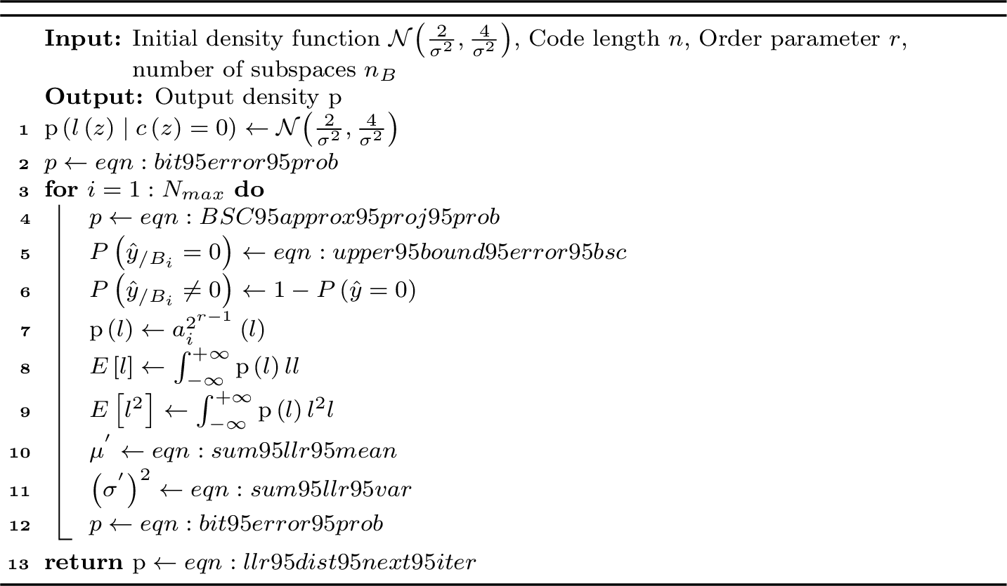
The pseudo-code of the density evolution of cpa decoding is shown in Algorithm [alg:density95evolution95PA]. We use the rm\(\left(7,3\right)\) code at \(E_\mathrm{b}/N_{0}=2.5\text{ dB}\), and the optimized and pcpa decoding with \(128\) subspaces [24], [37] and the broadcast update [22] to run the simulations. We first plot the number of occurrences of the received channel llr (iter. \(0\)) and the llr returned from each iteration of the pcpa decoding in Fig. 3. We can see that occurrences of the llr roughly follow Gaussian distributions. Hence, we plot the probability density function of the Gaussian distribution using the sample mean and variance of the llr in Fig. 4, which is denoted as “sim.” in the legend. Also, the probability density function of the Gaussian distribution using the computed mean \(\mu'\) and variance \(\left(\sigma'\right)^{2}\) is also plotted in Fig. 4. The probability density function of the Gaussian distribution returned from our proposed density evolution has a similar trend to the trend of the histogram in Fig. 3 and captures the mean- and variance-reduction feature, which explains the decoding mechanism behind cpa decoding.

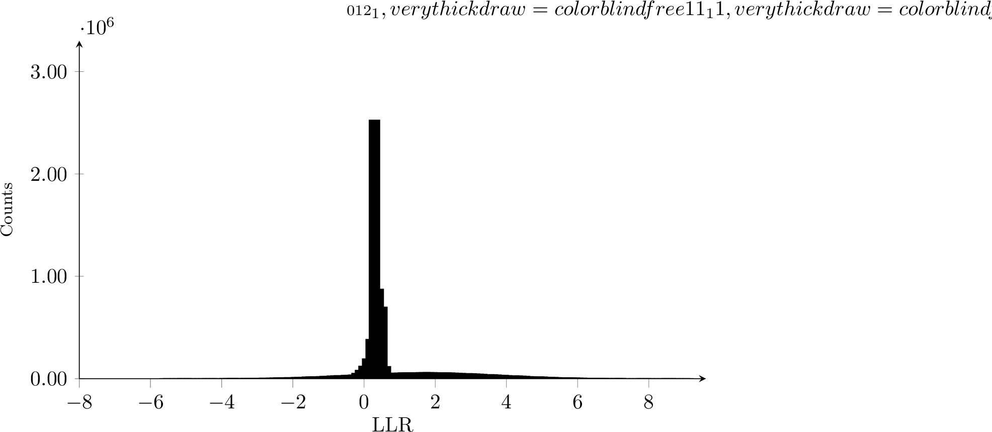
For the rm\(\left(8,3\right)\) code, the histogram of the llrs returned from the pcpa decoding with \(256\) subspaces and the broadcast update is shown in Fig. 5, and the density function returned from the empirical simulation is shown in Fig. 6. The llr values are more concentrated around the mean value compared to the histogram in Fig. 3 and the density functions in Fig. 4 for rm\((7,3)\) codes with \(128\) subspaces, which partially verifies the conjecture in 22 where a larger the number of subspaces implies a faster decay speed of error rates. Based on the saturation early stopping [19], [24], for two consecutive iterations, the difference in the L2 norm between returned soft information will be smaller than a threshold \(\theta\), and hard-decision results will be the same after a couple of iterations, which triggers the early stopping and explains the fast convergence speed.

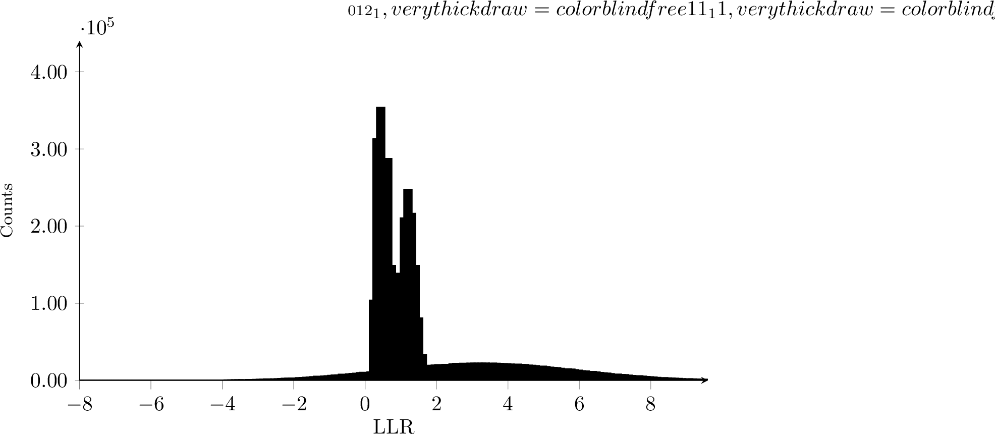
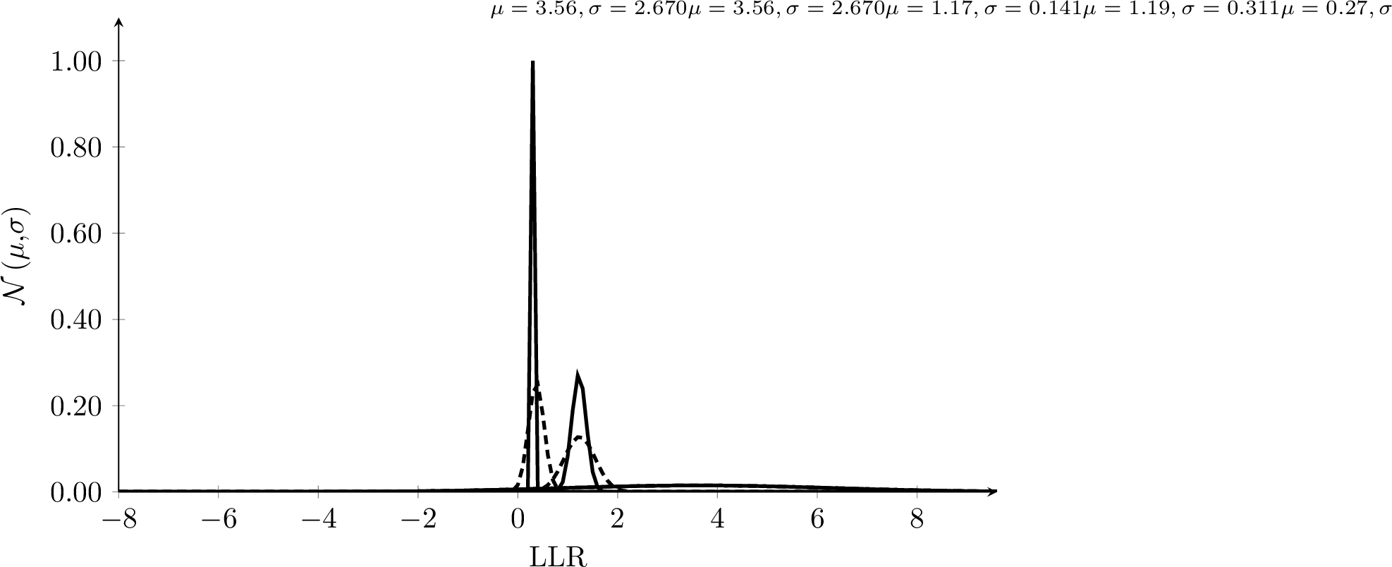
From Fig. 4, we can see that our derived lower bound \(\mu'\) is tight. The variance \(\left(\sigma'\right)^{2}/n_{\mathbb{B}}\) is underestimated because, at a finite code length, the output llrs at each iteration of the pcpa decoding are not necessarily independent across all subspaces, and the summation of two (dependent) random variables \(X_{1}\) and \(X_{2}\) has a variance of \(\sigma_{1}^{2}+\sigma_{2}^{2}+2\text{Cov}\left(X_{1},X_{2}\right)\) and this variance maybe larger than the variance \(\sigma_{1}^{2}+\sigma_{2}^{2}\) of our assumption that variables are independent. Hence, under the independent assumption and the proposed model, a useful bound for the decoding bit error 21 cannot be produced. Also, the distribution of the summation of dependent random variables is hard to analyze, unlike the distributions of independent random variables, and it may not be a normal distribution [38]. Furthermore, the interaction between dependent/correlated distributions returned from different subspaces is hard to analyze. In conclusion, a more fine-grained analysis (i.e., considering the dependency among subspaces) for the density evolution is needed for cpa decoding in future work to support analysis such as the bound for the decoding error.

The underestimation effect on the variance \(\left(\sigma'\right)^{2}/n_{\mathbb{B}}\) is also reflected in the iterative density evolution analysis on the rm\(\left(8,3\right)\) codes. From Fig. 6, the density evolution analysis returns a lower mean value than the mean value returned from the empirical simulation at iteration \(1\), which shows that our derived lower bound is tight for rm\(\left(8,3\right)\) codes, except for the mean value returned from the density evolution at iteration \(2\). It can be observed from Fig. 5 that most llrs are concentrated on several coarse-grained bins; hence, the empirical mean and the empirical standard deviation might not be accurate.

5 Asymptotic Analysis of cpa Decoding↩︎

In this section, the asymptotic analysis for cpa decoding with one decoding iteration is performed. The asymptotic analysis is based on the probabilistic model derived by our density evolution analysis for cpa decoding, and, in this work, we conduct the asymptotic analysis based on the asymptotic behaviour for all key operations. Combining the analytical results of the projection, the fht decoding, and the aggregation function, we derive the asymptotic behaviour.

5.1 Asymptotic Analysis of the Projection and fht Decoding↩︎

It is mentioned in [39], [40] that the ML decoding asymptotically decodes all but a vanishing fraction of error patterns of a weight up to \(\tfrac{n}{2}\left(1-\epsilon_{r}^{\min}\right)\) for low-rate RM codes with a fixed \(r\), and the residual term \[\lim_{m\rightarrow\infty}\epsilon_{r}^{\min}\left(m\right) = \lim_{m\rightarrow\infty}m^{r/2}n^{-1/2}\left(\frac{c\left(2^{r}-1\right)}{r!}\right)^{1/2}\text{,} \label{eqn:frac95nondecodeable95error95pattern}\tag{25}\] where \(c\) is a constant. For order-\(1\) RM codes, the residual term becomes \[\begin{align} \lim_{m\rightarrow\infty}\epsilon_{1}^{\min}\left(m\right)=&\lim_{m\rightarrow\infty}m^{1/2}n^{-1/2}\left(\frac{c\left(2^{1}-1\right)}{1!}\right)^{1/2}\\ &=\lim_{m\rightarrow\infty} \left(\frac{m}{2^{m}}\right)^{1/2}c^{1/2}\\ &\stackrel{(a)}{=}\lim_{m\rightarrow\infty}\left(\frac{1}{m2^{m-1}}\right)^{1/2}c^{1/2}=0\text{,} \end{align} \label{eqn:limit95correctable95error95patterns95FHT}\tag{26}\] where \(\left(a\right)\) in 26 holds by L’Hôpital’s rule. Hence, we can conclude that the fht decoding, which is ml decoding for order-\(1\) RM codes, can decode all but a vanishing fraction of error patterns of weights up to \(\tfrac{n}{2}\left(1-\lim_{m\rightarrow\infty}\epsilon_{1}^{\min}\right)=\tfrac{n}{2}\). Then, the probability of receiving soft information that can be correctly decoded by the fht decoding is \[\sum_{i=0}^{n/2}\binom{n}{i}\hat{p}^{i}\left(1-\hat{p}\right)^{n-i}\text{,}\] which is the cumulative probability of having at most \(\tfrac{n}{2}\) negative soft information, and \(\hat{p}\) is the error probability of projected soft information. In this work, we are interested in the asymptotic behaviour (i.e., \(n\rightarrow\infty\)) of received sequences that can be correctly decoded.

We can define a variable \(\mathsf{X}=\sum_{z\in\{0,1\}^{m-r+1}}\boldsymbol{x}\left(z\right)\) where \(\boldsymbol{x}\left(z\right)=\mathbb{1}\!\left(\boldsymbol{l}_{/\mathbb{B}_{i}}\left(z\right)<0\right)\) and the \(z\) is the index for the projected bit estimation. The random variable \(\boldsymbol{x}\left(z\right)\) takes value \(1\) with a probability of \(\hat{p}\) and value \(0\) with a probability of \(1-\hat{p}\). By the central limit theorem, the distribution of \(\mathsf{X}\) can be well approximated (normal approximation to the binomial distribution) by \(\mathbb{P}\left(\mathsf{X}\right)=\mathcal{N}\left(n\hat{p},n\hat{p}\left(1-\hat{p}\right)\right)\). The random variable \(\mathsf{X}=i\) is exactly the event where \(i\) out of \(n\) projected code bits take the value \(1\), which are the erroneous code bits. Hence, \[\sum_{i=0}^{n/2}\binom{n}{i}\hat{p}^{i}\left(1-\hat{p}\right)^{n-i} \approx \mathbb{P}\left(\mathsf{X}\leq \frac{n}{2}\right)\] as \(n\rightarrow\infty\). By defining the standardized variable \[\mathsf{Z}=\frac{\mathsf{X}-n\hat{p}}{\sqrt{n\hat{p}\left(1-\hat{p}\right)}}\] and \(\mathbb{P}\left(\mathsf{Z}\right)=\mathcal{N}\left(0,1\right)\), we have \[\mathbb{P}\left(\mathsf{X}\leq \frac{n}{2}\right)=\mathbb{P}\left(\mathsf{Z}\leq\frac{\sqrt{n}\left(1/2-\hat{p}\right)}{\sqrt{\hat{p}\left(1-\hat{p}\right)}}\right)\text{,}\] and \[\lim_{n\rightarrow\infty} \mathbb{P}\left(\mathsf{Z}\leq\frac{\sqrt{n}\left(1/2-\hat{p}\right)}{\sqrt{\hat{p}\left(1-\hat{p}\right)}}\right)= \begin{cases} 1\text{, if }\hat{p}<\frac{1}{2}\text{,}\\ 0\text{, if }\hat{p}>\frac{1}{2}\text{,}\\ \frac{1}{2}\text{, if }\hat{p}=\frac{1}{2}\text{.}\\ \end{cases} \label{eqn:asymptotic95FHT95block95error}\tag{27}\]

We assume that we are working on RM codes with a code rate \(R\leq C\), where \(C\) is the channel capacity. Let \(r'\) be the solution of \[C\geq\max_{r'\in \{0,1,...,m\}}\left(\sum_{i=0}^{r'} \binom{m}{i}\right)\frac{1}{n}\text{,}\] and we assume that we are working on RM codes with \(r\leq r'\). When \(r=m\), we have a perfect channel condition with a signal-to-noise ratio \(=\infty\), and the vanishing error probability is trivially achieved. Hence, we focus on the discussion on the finite signal-to-noise ratio, and \(r<m\).

Based on the projection function, we can see that the llr is \(<0\) when there is an odd number of received llrs in \(\boldsymbol{l}\) is \(<0\). The probability \(\hat{p}\) of projected llrs \(<0\), by 12 , is \[\begin{align} \hat{p} &=\frac{1}{2}\left(1-\left(1-2p\right)^{2^{r-1}}\right)\text{,} \end{align}\] \[\require{physics} p=\int_{-\infty}^{0}\frac{1}{\sqrt{2\pi \sigma^{2}}} \exp(-\frac{(y-1)^{2}}{2\sigma^{2}}) \dd{y}\text{,}\] and \(y\) is the received symbol from the channel. Under the assumption of a bounded variance in the awgn channel, we have \(p<1/2\). When \(p<1/2\), the probability of a projected llr \(<0\) is \(\hat{p}<1/2\) when the order parameter \(r<\infty\). Hence, the asymptotically achievable code rate is \[\begin{align} R = \lim_{m\rightarrow\infty}\frac{\sum_{i=0}^{r<\infty}\binom{m}{i}}{2^{m}} \leq\sum_{i=0}^{r<\infty}\frac{1}{i!}\lim_{m\rightarrow\infty}\frac{m^{i}}{2^{m}}=0\text{.} \end{align}\] Also, \(\lim_{m\rightarrow\infty}m-r+1=\infty\) for \(r<\infty\), 26 holds for the order-\(1\) sub-codes for cpa decoding, and fht decoding decodes all but a vanishing fraction of error patterns by 27 because \(\hat{p}<1/2\).

5.2 Asymptotic Analysis on the Aggregation Function↩︎

In the following theorem, we show that the random variable \(l\) has a positive mean and bounded variance when \(r<\infty\) and the input llr has a positive mean value.

By the sufficient condition of Theorem 1, the expected value \[\begin{align} \mathbb{E}\left[\tanh\left(\frac{\boldsymbol{l}\left(z\right)}{2}\right)\right]>0 \end{align}\] when the input llr has a positive mean \(\mathbb{E}\left[\boldsymbol{l}\left(z\right)\right]>0\). Because of the iid assumption on the transmitted code bits, it is shown in [28] that \[\begin{align} \mathbb{E}\left[\prod_{i=1}^{2^{r-1}-1}\tanh\left(\frac{l_{i}}{2}\right)\right] &= \mathbb{E}\left[\tanh\left(\frac{l_{i}}{2}\right)\right]^{2^{r-1}-1}>0 \end{align}\] when \(r<\infty\). Hence, by Theorem 1, \(\mathbb{E}[l]>0\) when \(r<\infty\).

According to ?? , the \(d\)-density can be converted to the \(l\)-density. Hence, the second-order moment of \(l=2\tanh^{-1}\left(d\right)\) can be computed by \[\require{physics} \begin{align} &\mathbb{E}\left[l^{2}\right]\\ &=\int_{-\infty}^{\infty} \mathrm{p}\left(l\right) l^{2} \dd{l}\\ &=\int_{-\infty}^{\infty} \mathrm{p}\left(\tanh\left(\frac{l}{2}\right)\right) \frac{l^{2}}{2\cosh^{2}\left(\frac{l}{2}\right)} \dd{l}\\ &\stackrel{(a)}{\leq} \int_{-\infty}^{\infty} \mathrm{p}\left(\tanh\left(\frac{l}{2}\right)\right) 4 \dd{l}=4\text{,}\\ \end{align} \label{eqn:l95density95with95d95density95variance95bound}\tag{30}\] the inequality \((a)\) in 30 holds because \[\begin{align} &\frac{l^{2}}{2\cosh^{2}\left(l\right)}\\ &= \frac{l^{2}}{2\sinh^{2}\left(\frac{l}{2}\right)}2\tanh^{2}\left(\frac{l}{2}\right)\\ &=\frac{2l^{2}}{\left(\exp\left(\frac{l}{2}\right) - \exp\left(-\frac{l}{2}\right)\right)^{2}}2\tanh^{2}\left(\frac{l}{2}\right)\\ &\stackrel{(b)}{\leq}\frac{2\left(\exp\left(\frac{l}{2}\right) + \exp\left(-\frac{l}{2}\right)\right)^{2}}{\left(\exp\left(\frac{l}{2}\right) - \exp\left(-\frac{l}{2}\right)\right)^{2}}2\tanh^{2}\left(\frac{l}{2}\right)\\ &=\frac{1}{\tanh^{2}\left(\frac{l}{2}\right)} 4\tanh^{2}\left(\frac{l}{2}\right)=4\text{,} \end{align}\] and the inequality \((b)\) holds because \[\begin{align} \left(\exp\left(\frac{l}{2}\right) + \exp\left(-\frac{l}{2}\right)\right)^{2}&= \left(2\cosh\left(\frac{l}{2}\right)\right)^{2}\\ &\stackrel{(c)}{=} 4\left(\sum_{i=0}^{\infty}\frac{\left(l/2\right)^{2i}}{\left(2i\right)!}\right)^{2}\\ &\stackrel{(d)}{\geq} 4 \left(1+\frac{l^{2}}{8}\right)^{2}\geq l^{2}\text{,} \end{align}\] where the equality \((c)\) holds by the definition of the Taylor series for the \(\cosh\left(\cdot\right)\) function, and the inequality \((d)\) holds by keeping only the first two terms of the series and truncating the rest. The bounded second-order moment (\(\mathbb{E}\left[l^{2}\right]\)) implies the first-order moment (i.e., expected value \(\mathbb{E}\left[l\right]\)) is also bounded. Hence, \[\begin{align} &\text{Var}\left[l\right]= \mathbb{E}\left[l^{2}\right] - \left(\mathbb{E}\left[l\right]\right)^{2}\leq 4 - \left(\mathbb{E}\left[l\right]\right)^{2} < \infty\text{.} \end{align} \label{eqn:sym95l95density95aggre95l95var95bound}\tag{31}\] Hence, when \(r<\infty\), the positive mean 29 , the bounded variance 31 , and the asymptotically vanishing error probability in the fht decoding 27 are returned from cpa decoding, and we can see that the random variable \(u\), which is defined in 14 , returned from the estimation for the aggregation based on a subspace \(\mathbb{B}_{i}\) asymptotically has \[\mathbb{E}\left[u\right]\stackrel{(a)}{=}\mathbb{E}\left[l\right]\text{, }\text{Var}\left[u\right]\stackrel{(b)}{=}\text{Var}\left[l\right]\text{,}\] and the equality \((a)\) holds because of 17 and the equality \((b)\) holds because of 19 . If the number of subspaces is asymptotically infinite, then, by 20 , the vanishing error probability can be achieved.

5.3 Asymptotic Analysis on the Number of Subspaces and the Asymptotic Behaviour of cpa Decoding↩︎

From 20 , we know that the averaging over the summation of the aggregation results is a form of variance reduction. Hence, if the number of subspaces \(\mathbb{B}_{i}\) goes to \(\infty\) as \(n\) goes to \(\infty\), cpa decoding will asymptotically achieve vanishing error probability. The following proposition shows that the number of subspaces can go to infinity as \(n\rightarrow\infty\).

The largest code rate that has an infinite number of subspaces can be computed as follows. The code rate of the rm\(\left(m,\tfrac{m}{q} +1\right)\) codes can be computed by \[\begin{align} \frac{\sum_{i=0}^{m/q+1}\binom{m}{i}}{2^{m}}&=\sum_{i=0}^{m/q+1}\binom{m}{i}0.5^{i}0.5^{m-i}\\ &=\mathbb{P}\left(i\leq \frac{m}{q}+1\right)\text{,} \end{align} \label{eqn:std95Chebyshev}\tag{32}\] which is the distribution function of the binomial distribution with a flipping probability of \(0.5\), a mean value of \(\tfrac{m}{2}\), and a variance of \(0.5^{2}m\). By the definition of the cumulative distribution, asymptotically, the largest code-rate, which has an infinite number of subspaces, is \[\begin{align} &\lim_{m\rightarrow\infty}\mathbb{P}\left(i\leq\frac{m}{q}+1\right)=\mathbb{P}\left(i\leq\infty\right)=1\text{.} \end{align} \label{eqn:limit95code95rate95cpa}\tag{33}\]

Given the analysis on the projection, fht decoding, and the aggregation function \(\left(r<m=\infty\right)\), the limiting code rate (\(R=\) 33 ), and the given channel capacity \(C\), we can conclude that, when code rate \(R\leq \min\left\{C,1,0\right\}=0\), cpa decoding can asymptotically achieve a vanishing error probability under the vanishing code rate.

6 Conclusion↩︎

We prove that cpa decoding returns the exact marginal probability and is symmetric. Then, we build a density evolution model to analyze cpa decoding. Simulation results show that our proposed density evolution model captures the fast reduction in the mean and the variance of the soft information returned from cpa decoding, and these results qualitatively explain the decoding mechanism and the fast convergence behind the CPA decoding. Lastly, we perform an asymptotic analysis on cpa decoding based on the proposed density evolution model, and we find that cpa decoding asymptotically achieves a vanishing error probability when decoding rm codes with a vanishing code rate. The analysis in this work provides tools and insights for designing soft-decision pa-based decoding with reduced complexity and improved decoding performance in future work.

References↩︎

---

1. Jiajie Li, Marvin Rübenacke, and Warren J. Gross are with the Department of Electrical and Computer Engineering, McGill University, Montréal, Québec, Canada. (e-mail: jiajie.li@mail.mcgill.ca; marvin.ruebenacke@mcgill.ca; warren.gross@mcgill.ca).↩︎