Higher-Order Programs with Indefinite Causal Orders: a Linear Approach to Coherent Control of Quantum Processes
January 01, 1970
Abstract
Processes with indefinite causal orders (ICOs), such as the quantum switch, are higher-order quantum processes that superpose the order in which quantum operations are performed. Such coherent control yields computational advantages but is not faithfully captured by existing quantum programming languages: either they are restricted to the unitary case, and thus cannot combine ICOs with measurement, or they treat coherent control nonlinearly. In both cases, they do not realize the full computational power of ICOs. We introduce a higher-order quantum functional language that supports general quantum computation, not merely the permutation of channels, and whose linear type system allows quantum control to be well-defined beyond the unitary case, on arbitrary quantum channels. We equip this language with a small-step operational semantics that synchronizes measurement outcomes across superposed branches, using device references and a memory function. We also give a denotational semantics by means of completely positive maps. With linearity as the only constraint, some well-typed terms would denote unphysical maps. We therefore impose a typing discipline that goes beyond linearity, and interpret programs in the causal category \(\mathbf{Caus}[\mathbf{CPM}]\), under which every well-typed program is physically meaningful, a property that can be checked statically and efficiently. We prove soundness, and study the language’s expressive power: it can express every quantum channel at first order, and at second order a large subclass of the so-called quantum circuits with quantum control (QC-QCs), containing the quantum switch. Last but not least, we show that this language is well-designed enough to be extended to the nonlinear setting with recursion.
1 Introduction↩︎
1.1 Context and Motivations↩︎
Coherent control, or quantum control, is a concept that has attracted significant attention in the development of quantum programming languages. It refers to the ability to express not only superpositions of data, but also superpositions of programs, which are typically controlled by a quantum state. A fundamental example of coherent control is the quantum switch [1]. The quantum switch is the higher order quantum process whose input is pair of quantum operations, say \(\mathcal{C}\) and \(\mathcal{D}\), and whose output is the operation that consists in applying \(\mathcal{D}\circ \mathcal{C}\) and \(\mathcal{C}\circ \mathcal{D}\) in a superposition, based on the state of a control qubit. The two programs in superposition are the two possible orderings of the input operations: \(\mathcal{C}\) before \(\mathcal{D}\) or \(\mathcal{D}\) before \(\mathcal{C}\). This is called an indefinite causal order.
Indefinite causal orders [2] are a subclass of coherent control that arises from higher-order quantum processes. They can be described as processes in which the ordering between a set of processes is in a superposition. Indefinite causal orders are of particular interest in quantum foundations [3]–[5], but have also been shown to grant an advantage in computational complexity in a variety of tasks [6]–[12]. A significant number of these examples use the quantum switch. Moreover, access to processes with indefinite causal orders can also provide advantages in some communication problems [13], [14] or information processing tasks [4].
Yet, existing quantum programming languages do not fully capture the expressive power of processes with indefinite causal orders. There are two major reasons for this.
Firstly, as we will argue in the paper, linearity is a key feature to implementing such processes. Processes with indefinite causal orders are linear by nature: the different orderings in superposition all have the same underlying set of
processes. However, programming languages that support coherent control often do so in a nonlinear fashion, which implements a closer analog to the classical if/then/else statement. Nonetheless, some processes with indefinite causal orders can
be simulated. For instance, in the unitary case, the quantum switch can be simulated by a quantum circuit in which one of the inputs is called twice [1]. However, due to using more resources, this implementation loses the potential computational advantages that the quantum switch would usually enable.
Secondly, integrating both indefinite causal orders and measurements into a quantum programming language is a non-trivial problem. In particular, the calculi in which quantum control is handled linearly do not feature measurement [15]–[17]. Fundamentally, the problem concerns synchronizing measurement outcomes occurring in different branches of a superposition. That is, a process with indefinite causal orders consists of a superposition of a set of processes being executed in different orders. If one of those processes contains a measurement, which is a probabilistic operation, the observed outcome must be the same in every branch. In particular, the simulation of the quantum switch where one input is used twice does not work beyond the unitary case for exactly this reason. The ability to implement measurements is necessary to express coherent control in its full generality. Remarkably, [11] demonstrated an exponential separation in quantum query complexity between models with indefinite causal orders and standard quantum circuits, and this advantage specifically requires non-unitary gates.
In this paper, we develop a higher-order programming language that faithfully implements a large class of processes with indefinite causal orders, accounting for the presence of measurements. Crucially, one can check statically in polynomial time (see Remark 2) whether a program represents a physically meaningful process.
1.2 Overview↩︎
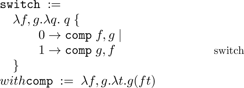
We give a brief overview of the design of the language and present its main features. The syntax of the language (Section 2) consists of the terms of the lambda calculus together with primitives implementing specific quantum features (including local unitaries, measurements and state initialisation). Quantum control is implemented with a dedicated \(\mathtt{qcase}\) primitive, written as \[\mathtt{qcase}\;P\;\{0\to M\;|\;1\to N\}.\] This program reads as follows. The term \(P\) represents a control qubit: if \(P\) evaluates to \(\ket{0}\), then \(M\) is executed; if \(P\) evaluates to \(\ket{1}\), then \(N\) is executed. If \(P\) evaluates to a superposition, then a coherent superposition of \(M\) and \(N\) is executed. The example of the quantum switch is given in Fig. 1. A linear typing discipline guarantees that any variables appearing freely in \(M\) or \(N\) must appear exactly once in \(M\) and exactly once in \(N\). It allows an indefinite-causal-order interpretation of higher order computations: roughly speaking, the same quantum channels are called in both \(M\) and \(N\) and only the order in which they are applied differs.
We endow this language with both operational (Section 3) and denotational semantics (Section 4).
1.2.1 Operational Semantics↩︎
In order to provide some intuition of the step-by-step execution of programs, let us consider the example of the quantum switch in more detail. The quantum switch is the higher order function whose input is a pair of quantum operations, given by variables \(f\) and \(g\), and whose output is a quantum operation acting on a pair of qubits \(q\) (“control”) and \(t\) (“target”). If the control qubit is in state \(\ket{0}\), \(f\) then \(g\) are applied to the target qubit. If it is in state \(\ket{1}\), \(g\) then \(f\) are applied to the target qubit. Otherwise, the two cases are executed in a coherent superposition depending on the state of the control qubit. This process can be summarized by the diagram in Figure 1, where the red dashed lines and the blue dash-dotted lines represent the two possible evolutions of the target qubit depending on the control qubit state. When the control qubit \(q\) is in state \(\ket{0}\), the target qubit \(t\) follows the red path. When the control qubit is in state \(\ket{1}\), the target qubit follows the blue path. Otherwise, the two alternative paths are in a superposition.
Consider its application \(\mathtt{switch}\;\pair{C,D}\;(H\ket{0})\;\ket k\) to a pair of operations \(\pair{C,D}\), with a control qubit in a superposition (\(H\) being the Hadamard gate), and with a target qubit in state \(\ket k\). Diagrammatically, the execution actually corresponds to two separate evolutions, represented as two alternative paths in a coherent superposition. This will be written using sums of terms. Therefore \(\mathtt{switch}\;\pair{C,D} \;(H\ket{0})\;\ket{k}\) will reduce, after a certain number of steps, to \[\begin{align} \label{eq:paths} \frac{1}{\sqrt{2}} \cdot {\color{red} \pair{ \ket{0}, D(C\ket{k})}} + \frac{1}{\sqrt{2}}\cdot {\color{blue} \pair{\ket{1},C(D\ket{k})} }. \end{align}\tag{1}\] where the first term of the superposition represents the red path with the control qubit in state \(\ket{0}\), and the second term represents the blue path with the control qubit in state \(\ket{1}\).
One of the main challenges we address is the combination of indefinite causal orders with measurements. Suppose that the input \(C\) contains a measurement (e.g., \(C=\mathtt{meas}\;P\;\{0\rightarrow M\;|\;1\rightarrow N\}\), for some \(P\), \(N\), and \(M\)). The two instances of \(C\) in (1 ) correspond to two distinct paths in which that same process appears, and not to two copies of the process; diagrammatically, the two copies of \(C\) correspond to the same box. Therefore, we expect the same measurement outcome for each copy of \(C\). To achieve this, we need to keep track of which identical subterms correspond to the same physical process. This is done by assigning a unique device reference to each measurement, which can be thought of as pointing to a specific physical device. To synchronize the measurement outcomes occurring in different branches of the superposition, we record measurement outcomes by means of a memory function, which is a partial function from device references to \(\{0,1\}\).
The operational semantics (Section 3) makes use of all these features: superpositions, device references, and memory functions, through the concept of configuration. It is important to note that superpositions of terms and device references are not actually accessible to the programmer, but rather serve as semantic tools to define the evolution of terms.
1.2.2 Denotational Semantics.↩︎
At first order, the most general evolutions from qubits to qubits are quantum channels, formally described as completely positive trace-preserving maps. They correspond to arbitrary compositions of unitary evolutions and measurements. At second order, the most general transformations from quantum channels to quantum channels are the quantum supermaps [1]. Iterating this construction yields quantum transformations of arbitrarily high order. Processes with indefinite causal orders, such as the quantum switch, can be described at the level of quantum supermaps.
We introduce a denotational semantics based on completely positive maps, which can be seen as morphisms of the category \(\mathbf{CPM}\). However, some higher-order morphisms of \(\mathbf{CPM}\) are not physically meaningful, in particular those that fail to satisfy the appropriate trace-preservation conditions. Such unphysical morphisms can be described by means of a non careful use of the \(\mathtt{qcase}\) construct (see Remark 7). To rule them out, we impose on \(\mathtt{qcase}\) a typing discipline that goes beyond linearity, so that only functions whose output consists of qubits can be coherently controlled. We then crucially rely on the \(\mathbf{Caus}\) construction [18] to prove that every well-typed term is physically meaningful. This denotational semantics provides a fine-grained treatment of the causal structure of quantum maps and supermaps. For instance, a value of type \((\text{\textrm{q}}\multimap\text{\textrm{q}})\otimes(\text{\textrm{q}}\multimap\text{\textrm{q}})\) need not be a pair of single-qubit channels, but may be an arbitrary no-signalling two-qubit channel [1]. Consequently, the quantum switch can be applied not only to pairs of single-qubit channels, but also to no-signalling two-qubit channel.
1.3 Summary of Contributions↩︎
In this paper, we define a higher-order functional programming language that supports indefinite causal orders and measurements. We give an operational semantics, which consists of a small-step transition system over configurations, i.e., superpositions of terms, and a denotational semantics in the category \(\mathbf{Caus}[\mathbf{CPM}]\). The language is shown to satisfy standard safety properties.
We prove the following main results:
1.3.1 Soundness Theorem↩︎
We prove that the denotational semantics is sound with respect to the operational semantics (Theorem [thm:soundness]): the reduction relation preserves the interpretation of terms.
1.3.2 Physicality of Programs↩︎
By construction, well-typed programs represent physically meaningful processes. This is because the denotational semantics can be defined not only in \(\mathbf{CPM}\), but also in the causal category \(\mathbf{Caus}[\mathbf{CPM}]\). Therefore, explicit connections can be made between types and collections of higher-order quantum maps.
It is especially interesting to relate this result to the operational semantics. In quantum programming languages based on superpositions of \(\lambda\)-terms, one of the main difficulties is checking that terms represent physically meaningful processes, typically unitary maps. This is generally achieved through orthogonality checks either at the price of sacrificing intensional completeness [19] or at the price of being undecidable [20]. Here, since superpositions of terms are not a feature that is accessible to the programmer, we will be considering sequences of reductions that start from a term without sums. Hence, the physicality of terms can be checked statically and efficiently: it suffices to check that the initial term is well-typed.
1.3.3 Expressivity↩︎
We study the expressivity of the language at the level of first-order and second-order functions. For first-order functions, we show that all quantum channels can be realized in the language (Proposition [prop:channels]). To study second-order functions, it is helpful to consider the expressivity of the language in comparison to the hierarchy of supermaps defined in [4], which we represent in Figure 2. The innermost class, Quantum Circuits with Fixed Causal Order, or QC-FOs, represents processes that do not have any control structure. The next class, Quantum Circuits with Classical Control, or QC-CCs, corresponds to processes fitting the “quantum data, classical control” paradigm [21]. The next class is Quantum Circuits with Quantum Control, or QC-QCs. This class contains all known examples of physically realizable processes with indefinite causal orders, including the quantum switch. Finally, QC-QCs do not encompass all existing supermaps—for instance the OCB process defined in [2] lies outside of the class of QC-QCs.
![Figure 2: The nested classes of supermaps defined in [4]](/article/2607.09534/_pdflatex/wihnmseb.png "fig:")
We prove that the language implements a subclass of QC-QCs that contains all QC-CCs, which we call QC-QCs with memory (Proposition [prop:qcqc]). This class contains the quantum switch and its direct generalizations [22], [23], but also some processes with dynamical control of causal orders—that is, processes where the orderings in a superposition are not fixed from the beginning and constructed on the fly.
1.3.4 An Extension for Non-Linearity and Recursion↩︎
Lastly, in Section 7 we extend the language to include nonlinear features and recursive functions. The ability to duplicate inputs is necessary to implement standard quantum algorithms whose inputs are oracles that are queried several times (for instance, [24]’s algorithm). Moreover, this enables us to define recursive functions, which will be considered duplicable. For example, this allows in to implement [25]’s “Repeat-Until-Success” circuits (Example 9). We show that the syntax and operational semantics can be extended to include both linear and nonlinear features in a straightforward way.
1.4 Related Work↩︎
There are numerous examples of quantum programming languages with coherent control, for instance [17], [19], [26]–[32]. In most cases, coherent
control is expressed as a quantum version of the classical if/then/else statement. Usually this primitive is called quantum case (“qcase”), quantum alternation or conditional, and corresponds to the process in which two branching programs are
executed in a superposition depending on the state of a control qubit. Generally, there is no linearity constraint between the then and else branches (although we point out that quantum control is treated linearly in [15], [16] in the absence of measurement). The lack of linearity constraint enables one to
write operations such as mapping a unitary gate to its controlled version. However, processes with indefinite causal orders cannot be faithfully implemented.
In fact, linearity is not just a means to implement processes with indefinite causal orders. At a more fundamental level, it allows quantum control itself to be well-defined. Indeed, without any linearity constraints, quantum control is defined on unitary maps by \((U,V)\mapsto \ket{0}\bra{0} \otimes U +\ket{1}\bra{1}\otimes V\). However, the extension of this semantics to completely positive maps is ill-defined [33]. For this reason, programming languages featuring both the nonlinear quantum case and measurements use semantic models such as Kraus decompositions [33]–[35] or vacuum-extended channels [36].
Operationally, coherent control can be implemented in models with superpositions of \(\lambda\)-terms [15], [16], [19], [20], [37]–[39]. In such calculi, one can write a unitary map directly from its matrix representation, which removes the need for built-in unitary gates. In fact, unitaries themselves are written as an instance of quantum control. The drawback is that verifying whether a term represents a physically meaningful process is generally difficult. To this end, it is necessary to define orthogonality constraints [15], [17], [26], where in particular, it was shown in [20] that deciding the orthogonality of terms is a \(\Pi^0_2\)-complete problem. Finally, [40]’s quantum \(\lambda\)-calculus, like ours, restricts sums to the topmost level of terms; however, its additional constraints on the shape of terms permit only classical control.
There exist several frameworks for the study of higher-order quantum maps [5], [41], [42]. The framework of causal categories [18] can be seen as a generalization to higher order of the trace-preserving condition for quantum channels. Another approach is presented in [43], which constructs a model guaranteeing the property of “total probability \(\leq 1\)” for higher-order programs.
2 Linear Language with Indefinite Causal Orders↩︎
In this section, we introduce the syntax and type system of a linear higher-order programming language for indefinite causal orders. We illustrate its expressiveness through several examples, including the quantum switch (Example 4).
2.1 Syntax↩︎
None
Figure 3: Syntax of the linear language for indefinite causal orders.
Let \(\mathcal{X}\) be a countably infinite set of linear variables, written \(x,y,z...\) The set of terms \(\mathscr{T}\) is defined by the grammar of Figure 3. The terms \(MN,\lambda x. M\) denote linear application and abstraction. The terms \(\pair{M,N}\) and \(\mathtt{let}\;\pair{x, y} = M \; \mathtt{in}\;N\) are the pair constructor and destructor, respectively. The term \(\text{\texttt{()}}\) is the unit. The sequence term \(M;N\) can be thought of as “\(\mathtt{let} \;\text{\texttt{()}}=M \;\mathtt{in} \;N\)”, meaning that the computation of \(M\) produces side effects and returns no meaningful value.
The term \(\mathtt{meas}\;P \;\{0\rightarrow M \;|\; 1\rightarrow N\}\) is used for expressing branching depending on the result of the measurement of a qubit \(q\). If the result of the measurement is \(0\), then \(M\) is executed, otherwise, \(N\) is executed. The term \(\mathtt{qcase}\;P \;\{0\rightarrow M\;|\;1\rightarrow N\}\) represents the superposition of terms controlled by \(P\). The terms \(\ket{0}\) and \(\ket{1}\) represent qubit states. \(U\) is any single qubit unitary transformation, i.e., \(U\in \mathbb{C}^{2\times 2}\) s.t. \(U^\dagger U=I\), \(I\) being the identity. Non-local unitary transformations can be reconstructed, for instance control-U can be defined as the following term \[\lambda x. \mathtt{qcase}\;x \;\{0\rightarrow I\;|\;1\rightarrow U\}.\]
By convention, application associates to the left, whereas pairs associate to the right. We identify terms up to \(\alpha\)-equivalence in a standard way. A term with no free variables is said to be closed. We define the following notations inductively, for all \(n\geq 2\): \[\begin{array}{rcl} \mathtt{let} \;x=M \;\mathtt{in}\;N &:= &(\lambda x . N)M \\ \mathtt{let} \;\pair{x_1,...,x_{n+1}} =M \;\mathtt{in}\;N &:= &\mathtt{let} \;\pair{x_1,y} =M \;\mathtt{in}\;\mathtt{let} \;\pair{x_2,...,x_{n+1}} =y \;\mathtt{in}\;N \\ \lambda \pair{x_1,...,x_n}. M & := & \lambda y. (\mathtt{let} \;\pair{x_1,...,x_n} = y \;\mathtt{in} \;M) \\ \ket{k_1,...,k_n} & := & \pair{\ket{k_1},...,\ket{k_n}} \quad \text{where }k_1,...,k_n\in\{0,1\} \end{array}\]
Lastly, we define the set of controllable terms \(\mathscr{C}\subseteq \mathscr{T}\) as the set of terms that do not contain measurement. Controllable terms are the only ones that can appear in the branches of a \(\mathtt{qcase}\) statement. This restriction is formalized by the type system in the following section.
2.2 Linear Type System↩︎
The type system is based on the multiplicative fragment of intuitionistic linear logic [44]. Types are given by the following syntax: \[\begin{array}{lll} \text{(Types)}\quad A,B \;& ::= \;& \text{\boldsymbol{1}}\;|\;\text{\textrm{q}}\;|\; A \otimes B \;|\;A \multimap B \end{array}\] \(\text{\boldsymbol{1}}\) is the unit type, and the ground type \(\text{\textrm{q}}\) represents a single qubit. \(A\otimes B\) is the linear product type. The type \(A \multimap B\) corresponds to linear functions. By convention, \(\multimap\) and \(\otimes\) associate to the right. We write \(\text{\textrm{q}}^n\) for \(\text{\textrm{q}}\otimes ... \otimes \text{\textrm{q}}\), where \(\text{\textrm{q}}\) appears \(n\geq 1\) times.
A typing context \(\Delta\) is a list of pairs of variables and their respective types \(x_1:A_1,...,x_n:A_n\), where \(x_1,...,x_n\) are pairwise distinct. Let \(\Delta\) and \(\Delta'\) be two typing contexts. If \(\Delta\) and \(\Delta'\) have no common linear variables, then we write \(\Delta, \Delta'\) for their union. Typing judgments are expressions of the following form: \[\Delta \vdash M :A\] where \(M\) is a term, \(A\) a type, and \(\Delta\) a typing context.
The typing rules are detailed in Figure 4. If a typing judgment can be derived using the typing rules, then it is said to be valid. A term \(M\) is said to be well-typed if there exist \(\Delta\) and \(A\) such that \(\Delta\vdash M:A\) is valid. Notice that in the meas and qcase rules, the typing context \(\Delta'\) is the same for both branching statements. In particular, if a typing judgment \(\Delta:M:A\) is valid, each variable of \(\Delta\) is guaranteed to appear exactly once in the term, where occurences in both branches of \(\mathtt{meas}\) or \(\mathtt{qcase}\) are counted as the same.
None
Figure 4: Typing rules. Recall that \(\mathscr{C}\) is the set of controllable terms, i.e., those without measurements..
The measurement statement is intended to discard the control qubit. To see this, notice that the type of \(\mathtt{meas}\;P\;\{0\to M\;|\;1\to N\}\) matches that of \(M\) and \(N\). On the contrary, the qcase statement preserves the control qubit. This is why the type of \(\mathtt{qcase}\;P\;\{0\rightarrow M\;|\;1\rightarrow N\}\) is \(A\multimap\text{\textrm{q}}^{n+1}\), where \(M\) and \(N\) are controllable terms of type \(A\multimap\text{\textrm{q}}^n\) for some \(n\geq 1\). This type may seem surprising at first glance. However, the naive typing approach, which would consist in assigning \(\mathtt{qcase}\;P\;\{0\rightarrow M\;|\;1\rightarrow N\}\) the type \(\text{\textrm{q}}\otimes B\) when \(M\) and \(N\) have type \(B\), raises some causality issues: as we will see in Section 3 (Remark 7), it would allow us to type terms that are not physical.
In the qcase rule, the requirement that the branching statements \(M\) and \(N\) be controllable is essential to defining the operational and denotational semantics. We emphasize that this restriction does not prevent us from expressing the coherent control of terms containing measurements. Via an abstraction, we can write terms such as \[\mathtt{let}\;x=(\lambda y. \mathtt{meas}\;y\;\{0\to \ket{0} | 1\to \ket{1} \}) \;\mathtt{in}\;\mathtt{qcase}\;q\;\{0\to x\;|\;1\to x\}\] which is well typed and can be interpreted as the coherent control of a measurement channel.1
Remark 1 (Linearity as a means of defining coherent control). We briefly discuss how a linear type system enables us to define coherent control. It is helpful to distinguish two variants of the qcase primitive appearing in various quantum programming language: the linear qcase, as discussed in this paper, and the nonlinear qcase. The nonlinear qcase consists of a statement \(\mathtt{qcase}\;x\; \{0\to M \;|\;1 \to N\}\) where the only constraint on \(M\) and \(N\) is that they be of the same type. When \(M\) and \(N\) compute the unitary maps \(U\) and \(V\), respectively, its semantics is given by \((U,V)\mapsto \ket{0}\bra{0}_{x}\otimes U+\ket{1}\bra{1}_{x}\otimes V\). This semantics however cannot be extended to completely positive maps [33].
The linear qcase consists in the same statement where \(M\) and \(N\) are additionally required to have exactly the same set of linear variables, and cannot contain measurements (see Figure 4). Adding the linearity constraint is enough for the process to be well defined on completely positive maps. For instance, this is the case of the quantum switch, where each branching statement contains one copy of each input channel. More generally, processes with indefinite causal orders correspond to this linear variant of qcase. For these reasons, our language will use the linear version of the quantum case, formally enforced by the linear type discipline of Figure 4.
Remark 2 (Tractability of type inference). As the rules of Figure 4 implement a simple-type discipline over a linear lambda-calculus, its type inference is known to be tractable (i.e., computable in polynomial time), as a direct consequence of [45].
2.3 Examples↩︎
We present various examples to illustrate the expressiveness of the language. The full typing derivations are given in Appendix [sec:app:examples].
Example 1 (CNOT). Non local unitary transformations can be constructed in the language, for instance the control-NOT gate is defined by the following term: \[\mathtt{CNOT} \;:= \;\lambda c.\mathtt{qcase}\;c \;\{0\rightarrow I \;|\;1\rightarrow X\}.\] One can derive the typing judgment \(\vdash \mathtt{CNOT}: \text{\textrm{q}}\multimap\text{\textrm{q}}\multimap\text{\textrm{q}}\otimes \text{\textrm{q}}\). Although only single-qubit unitary gates are built into the language’s syntax, this construction demonstrates that this restriction does not actually affect the language’s expressiveness. Indeed, CNOT and single-qubit unitary gates form a univeral set of gates [46].
Example 2 (Discard). The discard map is implemented by the following program: \[\mathtt{discard} \;:= \;\lambda c. \mathtt{meas}\;c\;\{0\rightarrow \text{\texttt{()}}\;|\;1\rightarrow \text{\texttt{()}}\}\] and can be typed as \(\vdash \mathtt{discard}: \text{\textrm{q}}\multimap\text{\boldsymbol{1}}\). Note that due to linearity, \(\mathtt{discard}\) could not have been written as \(\lambda c. \text{\texttt{()}}\).
Example 3 (Composition). The term \(\mathtt{comp}=\lambda \pair{f, g}.\lambda t. g(ft)\), provided in Figure 1, that simulates the composition can be given the type \((A\multimap B)\otimes (B\multimap C)\multimap A\multimap C\), for any types \(A\), \(B\), \(C\).
Example 4 (Quantum switch). Using the composition function, the quantum switch \(\mathtt{switch} \;:= \lambda \pair {x,y}. \lambda q. \mathtt{qcase}\;q\;\{0\rightarrow \mathtt{comp} \;\pair{x,y} \;|\;1\rightarrow \mathtt{comp} \;\pair{y,x}\}\) (also given in Figure 1) can be typed as: \[\vdash \mathtt{switch}: (\text{\textrm{q}}^n\multimap\text{\textrm{q}}^n)\otimes (\text{\textrm{q}}^n\multimap\text{\textrm{q}}^n )\multimap\text{\textrm{q}}\multimap\text{\textrm{q}}^n \multimap\text{\textrm{q}}^{n+1}\]
3 Operational Semantics↩︎
3.1 Design Choices↩︎
In this section, we describe the operational semantics for evaluating the terms of the language. The presence of controllable terms makes the definition of the operational semantics challenging, as, for instance, given \(\texttt{Meas}\;:= \;\lambda c. \mathtt{meas}\;c \;\{0 \to \ket{0} \;|\;1 \to\ket{1}\}\), a quantum switch on two copies of \(\texttt{Meas}\): \[\lambda \pair {x,y}. \lambda q. \mathtt{qcase}\;q\;\{0\rightarrow \mathtt{comp} \;\pair{x,y} \;|\;1\rightarrow \mathtt{comp} \;\pair{y,x}\}\;\pair{ \texttt{Meas}, \texttt{Meas}}\] is well typed but \(\lambda q. \mathtt{qcase}\;q\;\{0\to \mathtt{comp}\;\pair { \texttt{Meas}, \texttt{Meas}}~|~1\to \mathtt{comp}\;\pair { \texttt{Meas}, \texttt{Meas}}\}\) is not. As a consequence, the first term cannot reduce to the second in one or several steps. There is a fundamental reason for this: \(\mathtt{qcase}\;q\;\{0\to \mathtt{comp}\;\pair {x,y}~|~1\to \mathtt{comp}\;\pair {y,x}\}\) represents an indefinite causal order: the instrument \(x\) is performed first in one branch, last in the other. By contrast, the term \(\mathtt{qcase}\;q\;\{0\to \mathtt{comp}\;\pair { \texttt{Meas}, \texttt{Meas}}~|~1\to \mathtt{comp}\;\pair { \texttt{Meas}, \texttt{Meas}}\}\) does not witness which instrument is performed first, and is thus rejected by the typing rules. To preserve distinguishability while reducing the terms, we equip each measurement device with a unique identifier via device references. A second challenge in the definition of the operational semantics is the necessity of reducing both branches of a \(\mathtt{qcase}\) in superposition, so as to allow interference. To do so, we allow a term to reduce to a sum of terms (at the topmost level) to account for the superposition phenomenon. Thus, the operational semantics intuitively proceeds as follows: \[\begin{align} &\lambda \pair{x,y}. \lambda q. \mathtt{qcase}\;q\;\{0\to \mathtt{comp}\;\pair {x,y}~|~1\to \mathtt{comp}\;\pair {y,x}\}\;\pair{ \texttt{Meas}[d], \texttt{Meas}[e]} \;H\ket 1\;\ket k\\ &\quad \twoheadrightarrow^* \, \, \frac{1}{\sqrt 2} \cdot \pair{ \ket 0, \mathtt{comp}\;\pair {\texttt{Meas}[d],\texttt{Meas}[e]}\;\ket k}- \frac{1}{\sqrt 2} \cdot \pair{\ket 1, \mathtt{comp}\;\pair {\texttt{Meas}[e],\texttt{Meas}[d]}\;\ket k} \end{align}\] where \(\texttt{Meas}[i] := \lambda c. \mathtt{meas}\;i\triangleright c \;\{0 \to \ket{0} \;|\;1 \to\ket{1}\}\) and \(d,e\) are device identifiers. Additionally, the measurement outcomes associated with each device will be recorded in a memory function. This way, the two occurrences of \(\texttt{Meas}[d]\) (one in each branch of the superposition) share the device \(d\) and hence produce the same measurement outcome, while \(\texttt{Meas}[e]\) carries a different device \(e\) and thus produces an independent outcome.
3.2 A Language for Program Executions↩︎
In order to define the reduction of terms, we define a language for program executions, which is essentially the original set of terms \(\mathscr{T}\) to which we add device references and linear combinations of terms. These new features are not assumed to be accessible to the programmer, but are rather a tool to define the semantics of the language.
3.2.1 Adding Device References↩︎
The first step is to add device references. Let \(\mathbb{D}\) be a countably infinite set of device references, which we write as \(d,e,f\)... The set of execution terms \(\mathscr{E}\) is defined by the grammar in Figure 5.
None
Figure 5: Syntax of execution terms.
The only change compared to the set of terms \(\mathscr{T}\) (Figure 3) is the addition of a device reference \(d\) to the primitive for measurement. The set of device references appearing in an execution term \(M\) will be written as \(\text{Dev}(M)\). In order to type execution terms, the following typing rules are defined on terms of \(\mathscr{E}\): \[\scalebox{0.9}{ \begin{prooftree} \hypo{\Delta \vdash P:\text{\textrm{q}}} \hypo{\Delta' \vdash M:A} \hypo{\Delta' \vdash N: A} \infer3[meas]{\Delta,\Delta'\vdash \mathtt{meas}\;d\triangleright P\;\{0\rightarrow M\;|\;1\rightarrow N\}: A} \end{prooftree}} \quad \scalebox{0.9}{ \begin{prooftree} \hypo{\Delta \vdash P:\text{\textrm{q}}} \hypo{\Delta' \vdash M:A\multimap\text{\textrm{q}}^n} \hypo{\Delta' \vdash N: A\multimap\text{\textrm{q}}^n} \infer3[qcase]{\Delta,\Delta'\vdash \mathtt{qcase}\;P\;\{0\rightarrow M\;|\;1\rightarrow N\}: A\multimap\text{\textrm{q}}^{n+1}} \end{prooftree}}\] Namely, the typing rule for measurement with a device reference is similar to the rule (meas) of Figure 4, and in the rule for qcase, the hypothesis requiring that \(M\) and \(N\) be controllable is dropped. The rules for all other primitives are defined as being the same as those in Figure 4.
As usual, for \(M,N\in\mathscr{E}\) and \(x\in\mathcal{X}\), \(M\{N/x\}\) is the execution term obtained by replacing each occurrence of \(x\) in \(M\) by \(N\).
To define the operational semantics, a term \(M\in\mathscr{T}\) is lifted to an execution term by tagging its measurements with device references. A lifting of \(M\) is a term \(\lceil M \rceil\in\mathscr{E}\) obtained from \(M\) by assigning a distinct device reference to each measurement (and leaving \(M\) otherwise unchanged). Equivalently, \(\lceil M \rceil\) is any execution term whose measurements carry pairwise distinct references and which coincides with \(M\) once these references are erased. Liftings always exist and differ only in the choice of references.
Notice that if \(M\) is well-typed, then so is \(\lceil M \rceil\). However, the converse is false. This is because we have relaxed the assumption that branches of a \(\mathtt{qcase}\) statement are controllable. For example, the execution term \[\mathtt{qcase}\;x \;\{0\rightarrow \lambda t. \texttt{Meas}[d] \;(Ht) \;|\;1\rightarrow \lambda t. \texttt{Meas}[d] \;(Xt)\},\] with \(\texttt{Meas}[d]\) as in Section 3.1, is now well typed.
Remark 3. In practice, we can assume that the compiler automatically assigns unique device references as needed before executing the program.
To record the outcome of measurements occurring throughout the computation, we define memory functions. A memory function is a map \(\sigma\colon \mathbb{D}\to\{0,1\}_\bot\), where \(\{0,1\}_\bot:=\{0,1,\bot\}\) carries the flat order \(\preceq\) (\(\bot\preceq 0\), \(\bot\preceq 1\), with \(0\) and \(1\) incomparable) and such that the support \(\text{\textrm{Supp}}(\sigma):=\{\,d\in\mathbb{D}\mid\sigma(d)\neq\bot\,\}\) is finite. We write \(\mathcal{M}\) for the set of memory functions, ordered pointwise by \(\preceq\).
Definition 1 (Consistency). Two memory functions \(\sigma,\nu\) are consistent, written \(\sigma{||}\nu\), if they admit a common upper bound in \(\mathcal{M}\) — equivalently, if they agree on \(\text{\textrm{Supp}}(\sigma)\cap\text{\textrm{Supp}}(\nu)\). In that case their join \(\sigma\sqcup\nu:=\sup\{\sigma,\nu\}\) exists (the union of \(\sigma\) and \(\nu\) seen as partial maps).
We lift \(\sqcup\) to sets: for pairwise consistent \(\Theta,\Xi\subseteq\mathcal{M}\) (i.e.\(\sigma||\nu\) for all \(\sigma\in\Theta\), \(\nu\in\Xi\)), let \(\Theta\sqcup\Xi:=\{\,\sigma\sqcup\nu\mid\sigma\in\Theta,\;\nu\in\Xi\,\}\), and abbreviate \(\{\sigma\}\sqcup\Xi\) as \(\sigma\sqcup\Xi\). We write \([\bot]\) for the least memory function, mapping every device reference to \(\bot\). For \(d\in\mathbb{D}\) and \(k\in\{0,1\}\), we write \([d\mapsto k]\) for the function sending \(d\) to \(k\) and every other device reference to \(\bot\).
3.2.2 Adding Term Superpositions↩︎
In order to define the reduction rules, we must define linear combinations of terms. We define configurations, which allow term superpositions and are based on [15]’s notions of term distributions. The set of configurations, written as \(\vec{\mathscr{E}}\), is defined by the following grammar: \[\begin{array}{lrl} \text{(Configurations)} &\quad \vec{\mathscr{E}} \ni \vec{M},\vec{N} \;::= & \vec{0}\;|\;M^{\sigma}\;|\;\vec{M}+\vec{N} \;|\;\alpha \cdot \vec{M} \end{array}\] where \(M\in\mathscr{E}\), \(\alpha\in\mathbb{C}\), and \(\sigma\in\mathcal{M}\). The purpose of the memory function \(\sigma\) is to record all past measurement outcomes. In the particular case where \(\sigma=[\bot]\), we sometimes omit the superscript by writing \(M\) instead of \(M^{[\bot]}\) ; hence confusing the configuration with the execution term, by abuse of notation. The configuration or \(1 \cdot M^{[\bot]}\) is called an initial configuration, i.e., a configuration with amplitude \(1\) and least memory configuration. For simplicity, we also write \(M\) instead of \(1 \cdot M^{[\bot]}\).
Remark 4. We emphasize that linear combinations only appear at the topmost level of configurations. For example, instead of \((\lambda x. x) (\alpha\cdot \ket{0} +\beta\cdot \ket{1})\) we directly write \(\alpha\cdot (\lambda x. x) \ket{0} +\beta\cdot (\lambda x. x) \ket{1})\).
In Figure 6, we define a congruence relation \(\equiv\) over \(\vec{\mathscr{E}}\). The rules consist of all the axioms of a vector space except \(0\cdot\vec{M}=\vec{0}\). In technical terms, this corresponds to a weak vector space, which is also used in [15]’s calculus. The reason for excluding this rule is that even if a term cancels out, we must still keep the information of its memory function.
None
Figure 6: Congruence relation \(\equiv\).
We will now consider configurations up to \(\equiv\). Then by associativity, we can use the standard notation \(\sum_{i=1}^n \alpha_i\cdot M_i^{\sigma_i}\) for the sum \(\alpha_1 \cdot M_1^{\sigma_1} + ... + \alpha_n \cdot M_n^{\sigma_n}\). This allows us to define the canonical form of a configuration:
Definition 2 (Canonical form). The canonical form of a configuration \(\vec{M}\) is a configuration \(\sum_{i=1}^n \alpha_i \cdot M_i^{\sigma_i}\equiv \vec{M}\) such that the \(M_i^{\sigma_i}\) are pairwise distinct and the \(\alpha_i\) are (possibly 0) complex scalars. The canonical form is unique up to reordering of the terms of the sum.
The support of a configuration \(\vec{M}=\sum_{i=1}^n \alpha_i\cdot M_i^{\sigma_i}\) is defined as the set \(\text{\textrm{Supp}}(\vec{M}):=\{M_i^{\sigma_i}\}_{1\leq i\leq n}\). A configuration \(\vec{M}=\sum_{i=1}^n\alpha_i \cdot M_i^{\sigma_i}\) is said to be closed if every \(M_i\) is closed.
The following definition generalizes the concept of a term being well typed to configurations. In addition to requiring that each individual summand be well typed, we give some consistency conditions on the memory functions:
Definition 3 (Well-formedness). Let \(\vec{M}\) be a configuration whose canonical form is \(\sum_{i=1}^n \alpha_i \cdot M_i ^{\sigma_i}\). \(\vec{M}\) is said to be well formed* if the \(\sigma_i\) are pairwise consistent; and for all \(i\), \(M_i\) is well typed and \(\text{\textrm{Supp}}(\sigma_i)\cap \text{Dev}(M_i)=\emptyset\).*
Definition 4 (Memory of a configuration). For all well-formed configuration \(\vec{M}=\sum_{i=1}^n\alpha_i \cdot M_i^{\sigma_i}\), we define the memory of \(\vec{M}\) as \[\text{\textrm{Mem}}(\vec{M}): \sup_{1\leq i\leq n} \sigma_i\] where the supremum is taken with respect to \(\preceq\).
\(\vec{M}\) being well-formed ensures that the supremum is well defined. In particular, if \(\vec{M}\) and \(\vec{N}\) are well-formed configurations satisfying \(\text{\textrm{Mem}}(\vec{M})\;||\;\text{\textrm{Mem}}(\vec{N})\), then \(\vec{M}+\vec{N}\) is also well formed. Given a memory function \(\sigma\) and a well-formed configuration \(\vec{M}=\sum_{i=1}^n\alpha_i \cdot M_i^{\nu_i}\) such that \(\sigma \;||\;\text{\textrm{Mem}}(\vec{M})\), we define \(\vec{M}^{\{\sigma\}}:=\sum_{i=1}^n\alpha_i \cdot M_i^{\sigma\sqcup \nu_i}\).
3.3 Reduction Rules↩︎
The small-step semantics is a relation \({\twoheadrightarrow}\) over well-formed configurations \(\vec{M}=\sum_{i=1}^n\alpha_i \cdot M_i^{\nu_i}\in \vec{\mathscr{E}}\). It operates by reducing the individual execution terms \(M_i\in\mathscr{E}\) as initial configurations \(1 \cdot M_i^{[\bot]}\equiv M_i^{[\bot]}\). Each summand \(M_i\) carries its own memory function \(\nu_i\), whose support records the measurements performed so far in that summand; these supports may therefore differ from one summand of \(\vec{M}\) to another: the semantics should appropriately update memory functions while preserving consistency of the memory functions.
Before giving the reduction rules, we introduce some preliminary notions and notations. The set of values \(\mathscr{V}\) consists of execution terms defined by the following grammar: \[\begin{array}{lll} \text{(Values)} \quad \mathscr{V} \ni V,W \;::= \!\!\!\!& \;\;\; \lambda x. M \;|\;\text{\texttt{()}}\;|\;\pair{V,W} \;|\;U \;|\;\ket{0}\;|\;\ket{1} \end{array}\]
(Evaluation) contexts are defined by the following grammar: \[\begin{align} \text{(Contexts)} \quad E\;::=\;& [] \;| \;EV \;|\;ME\;|\;\pair{E,V}\;|\;\pair{M,E}\;|\;\mathtt{let}\;\pair{x,y}=E\;\mathtt{in}\;M\;|\;E;M \\ &\!\!\!\! |\;\;\mathtt{meas}\;d\triangleright E\;\{0\to M\;|\;1\to N\} \;|\;\mathtt{qcase}\;E\;\{0\to M\;|\;1\to N\} \end{align}\] where \(M,N \in \mathscr{E}\) and \(V \in \mathscr{V}\). Let \(E[M]\) be the execution term obtained when substituting \(M\) to \([]\) in \(E\). Contexts are extended to configurations through the following syntactic sugar: \[E\left[\sum_{i=1}^n \alpha_i \cdot M_i^{\sigma_i}\right] \;:=\;\sum_{i=1}^n \alpha_i \cdot E[M_i]^{\sigma_i}\]
The reduction relation \({\twoheadrightarrow} \subseteq \vec{\mathscr{E}}\times \vec{\mathscr{E}}\) is defined in Figure 7 for well-formed configurations. We remind you that the notation \(M \twoheadrightarrow \vec{M}\) means that \(M\) is an initial configuration. The reduction implements a call-by-basis reduction strategy, which is a special case of call-by-value in which the execution of terms is linear by construction [37].
None
Figure 7: Reduction relation \(\twoheadrightarrow\).
We now provide a some intuition on the rules of Figure 7.
The unitary rule \((un)\) is the one that introduces sums of terms. Namely, \(U\ket{k}\) reduces to a linear combination whose amplitudes are given by matrix components of \(U\).
Measurement statements are reduced by first evaluating the control term (here \(P\)). Then, if the control reaches a qubit state, we can either apply rule (\(m_0\)) or rule (\(m_1\)). Rule \((m_k)\) reads as follows: \(k\) is as the outcome of the measurement, and \(\ket{k'}\) is the state of the qubit being measured. If \(k\) and \(k'\) are different, then the result must be \(0\), hence the scalar \(\delta_{k,k'}\). The memory function records the measurement outcome obtained by the measurement device \(d\), which here is \(k\). Notice that (\(m_0\)), (\(m_1\)) and (\(sup\)) are the only rules that produce non-trivial memory functions.
Similarly, reductions of the qcase statement involve first reducing the control term (hence the first rule for the qcase). If the control is given by a qubit state \(\ket{k}\), this state must be preserved in the output. Therefore in the final term (in the second rule for the qcase), \(\ket{k}\) is paired with the corresponding branch \(M_k\), within a \(\lambda\)-abstraction.
In the case of an arbitrary configuration (rule \((sup)\)), the relation is defined by reducing one summand at a time. The memory functions of each summand are constructed on the fly by recording outcomes of measurements as they occur. Here, measurement statements in different summands that are assigned the same device should be understood as representing the same physical measurement. Therefore the outcomes occuring in each summand should be identical. This is formalized by the hypothesis \(\sigma \sqcup \text{\textrm{Mem}}(\vec{M})\;||\;\text{\textrm{Mem}}(\vec{N})\), which ensures that at each step of the reduction, the memory functions of each summand remain consistent. The hypothesis \(M^{\sigma}\notin \text{\textrm{Supp}}(\vec{N})\) indicates that we are reducing one of the summands of the canonical form. This is to avoid artificially constructing an infinite derivation, for instance by starting with \(M\equiv \frac{1}{2}\cdot M + \frac{1}{4}\cdot M+...\) and reducing the fractions one by one.
The reflexive transitive closure of \(\twoheadrightarrow\) will be written as \(\twoheadrightarrow^*\).
Notice that the operational semantics is nondeterministic: first, a transition from a configurations is obtained by applying a reduction rule to any one of its summands. Second, if the chosen summand is a measurement, there are two distinct applicable rules, corresponding to each measurement outcome.
Remark 5. Concretely, the reduction of a term \(M\in\mathscr{T}\) defined by the programmer will have the following form: \[\lceil M \rceil^{[\bot]} =\vec{N_0} \twoheadrightarrow \vec{N_1}\twoheadrightarrow \vec{N_2} \twoheadrightarrow \cdots\] where \(\lceil M \rceil\in\mathscr{E}\) and \(\vec{N_0},\vec{N_1},\vec{N_2}...\in\vec{\mathscr{E}}\). Treating the original set of terms \(\mathscr{T}\) and the set of configurations \(\vec{\mathscr{E}}\) as distinct has the following considerable advantage. Sums of terms allow us to express coherent control in a small-step transition system, and simultaneously, starting from a term of \(\mathscr{T}\) greatly simplifies checking that the computation is physically meaningful.
In quantum programming languages with linear combinations of terms, verifying unitarity, or more generally physicality, is known to be a major difficulty [15], [47]. Here, it is sufficient to check the initial term \(M\) is physical, which amounts to checking that it is well typed.2 In this case, the terms \(\vec{N_0},\vec{N_1},\vec{N_2},...\) will be considered physical on account of being reachable from \(M\). This will be further justified when we state the soundness theorem (Theorem [thm:soundness]) in Section 5.
Remark 6. Although device references were introduced in order to define the reduction of processes with indefinite causal orders, they can also be seen as a solution for treating the nonlinear measurement operation within a linear transition system. For instance, in the reduction \[\begin{align} \mathtt{meas}\;d\triangleright (H\ket{0}) \;\{0 \to M\;|\;1\to N\} &\twoheadrightarrow \frac{1}{\sqrt{2}}\cdot \mathtt{meas}\;d\triangleright \ket{0} \;\{0 \to M\;|\;1\to N\} \\ &\qquad + \frac{1}{\sqrt{2}}\cdot \mathtt{meas}\;d\triangleright \ket{1} \;\{0 \to M\;|\;1\to N\} \end{align}\] where \(H= \frac{1}{\sqrt{2}} \begin{psmallmatrix}1&1\\1&-1\end{psmallmatrix}\) is the Hadamard gate, the outcomes of the measurements in the two summands must be synchronized. Another solution for expressing measurement within a linear calculus is given in [38], [39], where the reduction strategy guarantees that measurements are treated consistently.
3.4 Examples↩︎
Example 5 (Quantum switch). We are now able to give an execution of the quantum switch. We consider the term \(\mathtt{switch} \;\pair{\texttt{Meas},\texttt{Meas}} \;(H\ket{0}) \;\ket{0}\), where \(H= \frac{1}{\sqrt{2}} \begin{psmallmatrix}1&1\\1&-1\end{psmallmatrix}\) is the Hadamard gate and the term \(\texttt{Meas}= \lambda c. \mathtt{meas}\;c\;\{0\to\ket{0}\;|\;1\to \ket{1}\}\) is taken from Section 3.1. The first step is to assign each measurement to a distinct measurement device (see Section 3.1). We will write this as \[\lceil \mathtt{switch} \;\pair{\texttt{Meas},\texttt{Meas}} \;(H\ket{0}) \;\ket{0} \rceil\;= \;\mathtt{switch} \;\pair{\texttt{Meas}[d],\texttt{Meas}[e]} \;(H\ket{0}) \;\ket{0},\] Then we have the following sequence of reductions:3 \[\begin{align} &\mathtt{switch} \;\pair{\texttt{Meas}[d],\texttt{Meas}[e]} \;(H\ket{0}) \;\ket{0}\\ &\quad \twoheadrightarrow^* \;\frac{1}{\sqrt{2}}\cdot \bigl(\lambda q. \mathtt{qcase}\;q\;\{0\rightarrow \mathtt{comp} \;\pair{\texttt{Meas}[d],\texttt{Meas}[e]} \;|\;1\rightarrow \mathtt{comp} \;\pair{\texttt{Meas}[e],\texttt{Meas}[d]} \}\bigr) \;\ket{0}\;\ket{0} \\ &\quad \quad \;\;+ \frac{1}{\sqrt{2}} \cdot \bigl(\lambda q. \mathtt{qcase}\;q\;\{0\rightarrow \mathtt{comp} \;\pair{\texttt{Meas}[d],\texttt{Meas}[e]} \;|\;1\rightarrow \mathtt{comp} \;\pair{\texttt{Meas}[e],\texttt{Meas}[d]} \}\bigr)\;\ket{1}\;\ket{0} \\ &\quad \twoheadrightarrow^* \;\frac{1}{\sqrt{2}}\cdot \lambda s. \pair{\ket{0}, \mathtt{comp} \;\pair{\texttt{Meas}[d],\texttt{Meas}[e]}\;s}\,\ket{0} +\;\frac{1}{\sqrt{2}} \cdot\lambda s. \pair{\ket{1}, \mathtt{comp} \;\pair{\texttt{Meas}[e],\texttt{Meas}[d]}\;s}\,\ket{0} \\ &\quad \twoheadrightarrow^* \;\frac{1}{\sqrt{2}}\cdot \pair{\ket{0}, \texttt{Meas}[e](\texttt{Meas}[d]\ket{0})} +\;\frac{1}{\sqrt{2}} \cdot\pair{\ket{1}, \texttt{Meas}[d](\texttt{Meas}[e]\ket{0})} \end{align}\]
Remark 7. In light of this example, we can explain our typing rule for the \(\mathtt{qcase}\) primitive (Figure 4) in more detail. One could opt for the following, perhaps simpler, rule: \[\scalebox{0.9}{ \begin{prooftree} \hypo{\Delta \vdash P:\text{\textrm{q}}} \hypo{\Delta' \vdash M:B} \hypo{\Delta' \vdash N: B} \hypo{M,N\in\mathscr{C}} \infer4[qcase]{\Delta,\Delta'\vdash \mathtt{qcase}\;P\;\{0\rightarrow M\;|\;1\rightarrow N\}: \text{\textrm{q}}\otimes B} \end{prooftree}}\] where the overall type is given by tensoring a qubit (for the output of the control) with the type of the branches. However this would enable the programmer to define unphysical terms. For example, the quantum switch term would reduce to a superposition of terms of the form \(\pair{\ket{k},M}\) where \(\ket{k}\) is the state of the control qubit. Then we could write: \[\mathtt{let}\;\pair{v,w}=\pair{\ket{k},M} \;\mathtt{in}\;wv\] Essentially, this term plugs the output of the control qubit into the input of the target qubit (see Figure 1). One can easily show that the corresponding process is unphysical, for instance by choosing as branching statements the Hadamard gate \(H\) and the phase gate \(S\).
An essential feature of our language is that typing alone should be enough to guarantee the physicality of a term. Hence we restrict the typing of \(\mathtt{qcase}\) by requiring that each branch have a type of the form \(A\multimap\text{\textrm{q}}^n\).
Example 6. The operational semantics works with the principle of synchronizing measurement outcomes occuring in different summands. Then, what happens if we force conflicting measurements outcomes in different branches of a \(\mathtt{qcase}\)? Consider the following program: \[\begin{align} \mathtt{N} \;:=&\;\left(\lambda w. \mathtt{qcase}\;H\ket{0} \;\{ 0 \rightarrow \lambda t. \pair{t,w\,\ket{0}} \;|\;1\rightarrow \lambda t.\pair{t,w\,\ket{1}}\}\right) \texttt{Meas}\;\ket{k} \end{align}\] where \(\texttt{Meas}\) is defined as in Section 3.1, \(H\) is the Hadamard gate, \(X\) the Pauli-\(X\) gate and \(k\in\{0,1\}\). In the 0 branch (resp. the 1 branch), the measured qubit is in state \(\ket{0}\) (resp. \(\ket{1}\)), therefore the measurement outcome should be \(\ket{0}\) (resp. \(\ket{1}\)). We write \(\mathtt{N'}:= \lceil \mathtt{N} \rceil^{[\bot]}\). Depending on the measurement outcomes, we have the two alternative reductions:4 \[\begin{align} \mathtt{N'} \twoheadrightarrow^* &\;\frac{1}{\sqrt{2}}\cdot \pair{\ket{0},\ket{k},\ket{0}}^{[d\mapsto 0]} + 0\cdot \pair{\ket{1},\ket{k},\ket{0}}^{[d\mapsto 0]} \\ \mathtt{N'} \twoheadrightarrow^* &\;0 \cdot \pair{\ket{0},\ket{k},\ket{1}}^{[d\mapsto 1]} + \frac{1}{\sqrt{2}} \cdot \pair{\ket{1},\ket{k},\ket{1}}^{[d\mapsto 1]} \end{align}\] Here the control qubit is the first qubit of the triple. Since each term only has one non-zero summand, we can conclude that forcing conflicting measurements equivalent to measuring the control qubit.
3.5 Properties of the Operational Semantics↩︎
3.5.1 Safety Properties↩︎
The language satisfies the following standard safety properties.
lemmalemsubstitution Let \(M,N\in\mathscr{E}\). Suppose \(\Delta_1,x:A,\Delta_2 \vdash M:B\) and \(\Delta_3 \vdash N:A\) are valid typing judgments such that \(\Delta_1,\Delta_2\) and \(\Delta_3\) have no variables in common. Then \(\Delta_1,\Delta_2,\Delta_3\vdash M\{N/x\}:B\) is a valid typing judgment.
The statement is proved by structural induction on the derivation of \(\Delta_1,x:A,\Delta_2 \vdash M:B\). Consequently, the language enjoys the usual subject reduction property:
propositionpropsubjectreduction Let \(M\in\mathscr{E}\). If \(\Delta\vdash M:A\) is a valid typing judgment and \(M\twoheadrightarrow \sum_i \alpha_i \cdot M_i^{\sigma_i}\), then for all \(i\), \(\Delta\vdash M_i:A\) is a valid typing judgment.
This is proved by induction on the derivation of \(M\twoheadrightarrow \sum_i \alpha_i \cdot M_i^{\sigma_i}\).
To prove progress, it is convenient to give the following definition:
Definition 5 (Final configuration). Let \(\vec{M}=\sum_{i=1}^n \alpha_i\cdot M_i^{\sigma_i}\) be a well-formed configuration. \(\vec{M}\) is said to be a final configuration* if for all \(i\in \{ 1,\ldots,n\}\), \(M_i\in\mathscr{V}\). The set of final configurations will be written as \(\vec{\mathscr{V}}\).*
lemmalemprogress
For all well-typed closed term \(M\in\mathscr{E}\), either \(M\in\mathscr{V}\) or there exists a reduction \(M\twoheadrightarrow \vec{M}\).
For all well-formed closed configuration \(\vec{M}\), either \(\vec{M}\in\vec{\mathscr{V}}\) or there exists a reduction \(\vec{M}\twoheadrightarrow \vec{M'}\).
3.5.2 Uniqueness of the Normal Form↩︎
In this section, we consider configurations \(\vec{M}\) that can be reduced to a given final configuration \(\vec{V}\). There are two sources of nondeterminism in the reduction relation \(\twoheadrightarrow\): the choice of summand to be reduced, and the choice of measurement outcome. When it comes to the choice of summand, we show uniqueness of the normal form. More precisely, suppose we have a configuration \(\vec{M}\). Given a fixed set of measurement outcomes for all devices of \(\text{Dev}(\vec{M})\), if \(\vec{M}\) is a normalizing term, then all reductions from \(\vec{M}\) lead to the same final configuration. This is formalized by the following confluence-like property:
propositionpropconfluence Suppose that \(\vec{M}\twoheadrightarrow^* \vec{N}\) and \(\vec{M}\twoheadrightarrow^* \vec{V}\), where \(\vec{V}\in\vec{\mathscr{V}}\) and \(\text{\textrm{Mem}}(\vec{N})\;||\;\text{\textrm{Mem}}(\vec{V})\). Then we have \(\vec{N}\twoheadrightarrow^*\vec{V}\). Diagrammatically, \[\scalebox{0.9}{ \begin{tikzcd}[ampersand replacement=\&] \&\vec{M} \ar[dl,twoheadrightarrow,"*"'] \ar[dr,twoheadrightarrow,"*"] \& \\ \vec{N} \ar[rr,twoheadrightarrow,dashed,"*"] \&\&\vec{V} \end{tikzcd}}\]
The consistency condition between the memory functions of \(\vec{N}\) and \(\vec{V}\) is necessary because the result only applies when measurement outcomes in either branch are not in contradiction. Therefore, for the same measurement outcomes, the value distribution to which a term can be reduced (when it exists) is unique up to congruence.
4 Denotational Semantics↩︎
To define the denotational semantics, we give separate interpretations for the set of controllable terms \(\mathscr{C}\) and the set of all terms \(\mathscr{T}\). Controllable terms, which are deterministic, are given a denotational semantics \([\cdot]\) in the category of finite-dimensional Hilbert spaces \(\mathbf{FHilb}\) (Section 4.2). The full denotational semantics is based on the Caus construction [18]. Specifically, the interpretation is defined in \(\mathbf{Caus}[\mathbf{CPM}]\), where \(\mathbf{CPM}\) is the category of completely positive maps (Section 4.3).
4.1 Compact Closed Categories↩︎
The denotational semantics will be defined in terms of symmetric monoidal categories (SMCs). An SMC \((\mathsf{C},\otimes,I)\) is a category equipped with a parallel composition operation \(\otimes\) for objects and morphisms, a unit object \(I\) and a swap morphism \(\gamma_{A,B}\) for all objects \(A,B\) satisfying some consistency equations. In this paper, SMCs will always be assumed to be strict, that is, satisfying the equalities \((A\otimes B)\otimes C = A\otimes (B\otimes C)\) and \(A\otimes I = A = I\otimes A\). We note that every SMC is equivalent to a strict one [48].
Definition 6 (Symmetric monoidal closed category). A symmetric monoidal closed category* (SMCC) is a symmetric monoidal category \((\mathsf{C},\otimes,I)\) such that for every object \(B\), the functor \(-\otimes B : \mathsf{C}\to\mathsf{C}\) has a right adjoint \(B\multimap-:\mathsf{C}\to\mathsf{C}\). We will write the corresponding bijections as: \[\phi_{A,B,C}: \mathsf{C}(A\otimes B,C)\cong \mathsf{C}(A,B\multimap C).\]*
We will omit the subscript \(A,B,C\) of \(\phi_{A,B,C}\) when the objects involved are clear from the context.
Compact closed categories are a particular case of SMCCs:
Definition 7 (Compact closed category). An SMC \(\mathsf{C}\) is said to be compact closed* if every object has a dual object \(A^*\), i.e. there exist morphisms \(\eta_A:I \to A^*\otimes A\) and \(\epsilon_A:A\otimes A^* \to I\) satisfying: \[(\epsilon_A\otimes 1_A)\circ(1_A\otimes \eta_A) = 1_A \qquad (1_{A^*}\otimes \epsilon_A)\circ(\eta_A\otimes 1_{A^*})=1_{A^*}\]*
As in [18], we assume the equalities \(I^*=I\), \(A^{**}=A\) and \((A\otimes B)^*=A^*\otimes B^*\) throughout. This is without loss of generality: in any compact closed category these three identifications are canonical and coherent [49], so every compact closed category is monoidally equivalent to one in which they hold strictly.
The morphisms \(\epsilon_A\) and \(\eta_A\) will be represented diagrammatically with cups and caps, respectively, so that the above equations can be written as: \[\scalebox{0.9}{ \tikzfig{eq_A}\;= \;\tikzfig{id_A} \qquad \tikzfig{eq_A_star} \;= \;\tikzfig{id_A_star} }\]
To see that every compact closed category is an SMCC, we choose the functor \(B\multimap-\) to be that defined by \(B\multimap C:=B^*\otimes C\) for all object \(C\), and \(B\multimap f:=1_{B^*}\otimes f\) for all morphism \(f:C\to C'\); together with the bijections \[\phi_{A,B,C}\left(\scalebox{0.9}{\tikzfig{f_bis}}\right) \;= \;\scalebox{0.9}{\tikzfig{phi_f_bis}} \qquad \phi_{A,B,C}^{-1}\left(\scalebox{0.9}{\tikzfig{g_bis}}\right) \;= \;\scalebox{0.9}{\tikzfig{phi_g_bis}}\] for all objects \(A,B,C\), where \(\scalebox{0.9}{\tikzfig{cap}}\;:= \;\scalebox{0.9}{\tikzfig{cap2}}\).
4.2 A Semantics of Controllable Terms↩︎
4.2.1 Higher-Order Linear Maps↩︎
Controllable terms will be interpreted in \(\mathbf{FHilb}\), the category of finite dimensional Hilbert spaces and \(\mathbb{C}\)-linear maps between them. The set of linear maps from a Hilbert space \(\mathcal{H}\) to a Hilbert space \(\mathcal{K}\) will be written as \(\mathcal{L}(\mathcal{H},\mathcal{K})\). \(\mathbf{FHilb}\) is a symmetric monoidal category, where \(\otimes\) is the usual tensor product, and is compact closed. The dual of an object \(\mathcal{H}\) is the Hilbert space \(\mathcal{H}^*\) of linear forms on \(\mathcal{H}\). For any \(\mathcal{H} \in \mathbf{FHilb}\), \(\eta_\mathcal{H}\) and \(\epsilon_\mathcal{H}\) are given by: \[\eta_\mathcal{H}: 1\mapsto \sum_i \ket{i}_{\mathcal{H}^*}\otimes\ket{i}_{\mathcal{H}} \qquad \epsilon_{\mathcal{H}}: \ket{i}_{\mathcal{H}}\otimes \ket{j}_{\mathcal{H}^*} \mapsto \braket{j}{i}_\mathcal{H} = \braket{i}{j}_{\mathcal{H}^*}\] where \((\ket{i}_{\mathcal{H}})_i\) is an orthonormal basis of \(\mathcal{H}\) and \((\ket{i}_{\mathcal{H}^*})_i\) is the corresponding dual basis of \(\mathcal{H}^*\). The definitions of \(\eta_\mathcal{H}\) and \(\epsilon_{\mathcal{H}}\) are independent of the choice of basis. The compact closed structure of \(\mathbf{FHilb}\) enables us to define a semantics for higher order linear maps. This is the same structure as that given by the Choi-Jamiołkowski (CJ) isomorphism [50], [51].
4.2.2 Interpretation in \(\mathbf{FHilb}\)↩︎
Controllable terms \(\mathscr{C}\) are given an interpretation \([\cdot]\):
to each type \(A\) we assign an object \([A]\) of \(\mathbf{FHilb}\): \[\begin{align} [\text{\boldsymbol{1}}] & := I = \mathbb{C} & [A\otimes B] & := [A]\otimes [B] \\ [\text{\textrm{q}}] & := \mathbb{C}^2 & [A\multimap B] &:= [A]\multimap[B] \end{align}\]
to each typing context \(\Delta = x_1:A_1,...,x_n:A_n\) we assign the object \([\Delta]:= [A_1]\otimes ... \otimes [A_n]\);
to each valid typing judgment \(\Delta\vdash M:A\) we assign a morphism \([\Delta]\to[A]\). The interpretation is defined in Figure 8, by induction on the derivation of the typing judgments. For the qcase rule, we define \(\mathfrak{q}(f,g):[\text{\textrm{q}}]\otimes[\Delta']\to [A\multimap\text{\textrm{q}}^n]\) as follows, for \(f,g:[\Delta']\to [A\multimap\text{\textrm{q}}^n]\): \[\mathfrak{q}(f,g) := (\gamma_{[\text{\textrm{q}}],[A]^*}\otimes I_{[\text{\textrm{q}}^n]})(\ket{0}\bra{0}\otimes f + \ket{1}\bra{1}\otimes g).\]
None
Figure 8: Denotational semantics of controllable terms.
We briefly explain the semantics for the qcase rule. Fix linear maps \(f,g:[\Delta']\to[A\multimap\text{\textrm{q}}^n]\). The controlled statements are not \(f\) and \(g\) themselves, but rather \(\phi^{-1}(f),\phi^{-1}(g):[\Delta']\otimes [A] \to[\text{\textrm{q}}^n]\), where the input on \([\Delta']\) can be seen as representing some parameters for the free variables of the branching statements \(M\) and \(N\). Therefore, the qcase statement is given by the linear map below: \[\ket{0}\bra{0}\otimes \phi^{-1}(f) + \ket{1}\bra{1} \otimes \phi^{-1}(g)\;:\;[\text{\textrm{q}}]\otimes [\Delta']\otimes [A] \to [\text{\textrm{q}}^{n+1}],\] which we will represent as \[\mathfrak{q}(f,g)\;:= \phi\bigl(\ket{0}\bra{0}\otimes \phi^{-1}(f) + \ket{1}\bra{1} \otimes \phi^{-1}(g)\bigr)\;:\;[\text{\textrm{q}}]\otimes [\Delta'] \to [A]\multimap[\text{\textrm{q}}^{n+1}].\] This expression can be simplified to \[\mathfrak{q}(f,g)\;= (\gamma_{[\text{\textrm{q}}],[A]^*}\otimes I_{[\text{\textrm{q}}^n]})\circ (\ket{0}\bra{0}\otimes f + \ket{1}\bra{1} \otimes g).\]
propositionproppurewelldefined The interpretation \([\cdot]\) is well-defined.
Due to the exchange rule, the derivation of a judgment is generally not unique. The proof of well-definedness involves showing that the interpretation is independent of the choice of derivation.
4.3 A Causal Semantics↩︎
4.3.1 Higher-Order Quantum Maps and Causal Categories↩︎
The full fragment will be interpreted in the category \(\mathbf{Caus}[\mathbf{CPM}]\). First, \(\mathbf{CPM}\) is the category of finite-dimensional Hilbert spaces and completely positive maps. We recall that a map \(\mathcal{C}\in\mathcal{L}(\mathcal{L}(\mathcal{H}),\mathcal{L}(\mathcal{K}))\) is completely positive if for all auxiliary Hilbert space \(\mathcal{E}\) and all positive matrix \(\rho\in\mathcal{L}(\mathcal{H}\otimes \mathcal{E})\), the matrix \((\mathcal{C}\otimes \mathcal{I}_{\mathcal{E}})(\rho)\in \mathcal{L}(\mathcal{K}\otimes\mathcal{E})\) is also positive. Like \(\mathbf{FHilb}\), the category \(\mathbf{CPM}\) is a symmetric monoidal category, with \(\otimes\) the usual tensor product. Moreover, \(\mathbf{CPM}\) is compact closed, with dual objects defined as dual vector spaces, and cups and caps defined by \[\eta'_\mathcal{H}: 1\mapsto \sum_{i,j} \ket{i}_{\mathcal{H}^*}{}_{\mathcal{H}^*}\bra{j}\otimes\ket{i}_{\mathcal{H}}{}_{\mathcal{H}}\bra{j} \qquad \epsilon_{\mathcal{H}}': \rho \mapsto \left(\sum_i {}_{\mathcal{H}} \bra{i}\otimes {}_{\mathcal{H}^*}\bra{i}\right)\,\rho\,\left(\sum_i \ket{i}_{\mathcal{H}}\otimes\ket{i}_{\mathcal{H}^*}\right)\] Further, there exists a identity-on-objects functor \(D:\mathbf{FHilb}\to \mathbf{CPM}\) that “doubles” linear maps to construct completely positive ones, that is \(D(f) = [\rho \mapsto f\rho f^\dagger]\). \(D\) preserves the compact closed structure of \(\mathbf{FHilb}\). In particular, we have \(D(f\otimes g)=D(f)\otimes D(g)\), \(D(\eta_{\mathcal{H}})=\eta'_{\mathcal{H}}\) and \(D(\epsilon_{\mathcal{H}})=\epsilon'_{\mathcal{H}}\).
Similarly to \(\mathbf{FHilb}\), the compact closed structure in \(\mathbf{CPM}\) corresponds the Choi-Jamiołkowski isomorphism in quantum theory5, which plays an important role in representing higher-order quantum maps. Quantum supermaps are defined as higher-order linear maps that send quantum channels to quantum channels, including when tensored with an identity map [1]. Via the CJ isomorphism, a quantum supermap can be transformed into a linear map that sends CJ representations of quantum channels to CJ representations of quantum channels. It was shown that such a linear map is completely positive [1]. In turn, its CJ representation is a positive-semidefinite matrix. By this process, all higher-order quantum maps can be represented as positive semidefinite matrices, and therefore in the category \(\mathbf{CPM}\).
Although it is remarkable that compact closure collapses all higher-order quantum maps to order 1, the disadvantage is that there is no way to keep track of whether maps are trace preserving (or trace preserving preserving, and further variations). A solution to this problem has already been studied in [18]: causal categories. We give a short summary of the construction.
A precausal category is defined as a compact closed category \(\mathsf{C}\) satisfying four additional axioms. Notably, \(\mathsf{C}\) is required to have discarding maps \(\mathfrak{d}_A \in\mathsf{C}(A, I)\) for each object \(A\), which are compatible with the monoidal structure. E.g., \(\mathbf{CPM}\) is a precausal category, whose discard maps are traceout functions. Given a precausal category \(\mathsf{C}\), the causal category \(\mathbf{Caus}[\mathsf{C}]\) is constructed as follows:
Definition 8. [18] Let \(\mathsf{C}\) be a precausal category. The dual of a set \(c\subseteq \mathsf{C}(I,A)\) is defined as \[c^*:= \left\{ \pi\in\mathsf{C}(I,A^*)\;\middle|\; \forall \rho \in c:\epsilon_A \circ (\pi\otimes \rho) \;= 1_I\right\}\] A set \(c\in\mathsf{C}(I,A)\) is closed* if \(c=c^{**}\) and flat if there exist invertible \(\lambda,\mu\in\mathsf{C}(I,I)\) such that \(\lambda \mathfrak{d}_A\in c\) and \(\mu \mathfrak{d}^*_A\in c^*\), where \(\mathfrak{d}_A^*\) is the transpose of \(\mathfrak{d}_A\), i.e \(\mathfrak{d}_A^*:=(\mathfrak{d}_{A^*}\otimes 1_A)\circ\eta_A\).6 \(\mathbf{Caus}[\mathsf{C}]\) is defined as the category whose objects are pairs \(\mathbf{A}=(A,c_\mathbf{A})\) where \(A\) is an object of \(\mathsf{C}\) and \(c_\mathbf{A}\subseteq \mathsf{C}(I,A)\) is closed and flat. Morphisms \(A\stackrel{f}{\to}B\) in \(\mathbf{Caus}[\mathsf{C}]\) are morphisms \(A\stackrel{f}{\to}B\) in \(\mathsf{C}\) such that \(\rho \in c_\mathbf{A} \Rightarrow f\circ \rho \in c_\mathbf{B}\).*
Tensor products are defined in \(\mathbf{Caus}[\mathsf{C}]\) as follows. Given objects \(\mathbf{A}=(A,c_\mathbf{A})\) and \(\mathbf{B}=(B,c_\mathbf{B})\) of \(\mathbf{Caus}[\mathsf{C}]\), we define \[c_\mathbf{A}\otimes c_\mathbf{B} := \{\rho_1\otimes \rho_2 \;|\;\rho_1\in c_\mathbf{A} \text{ and }\rho_2\in c_\mathbf{B}\}.\] Then, \(\mathbf{A}\otimes\mathbf{B}:=(A\otimes B,c_{\mathbf{A}\otimes \mathbf{B}})\) where \(c_{\mathbf{A}\otimes \mathbf{B}}:=(c_\mathbf{A}\otimes c_\mathbf{B})^{**}\). Equipped with this tensor product, \(\mathbf{Caus}[\mathsf{C}]\) is shown to be a symmetric monoidal category. Moreover, duals are defined as \(\mathbf{A}^*:=(A^*,c_{\mathbf{A}^*})\) with \(c_{\mathbf{A}^*}:=c_\mathbf{A}^*\). With \(\mathbf{A}\multimap\mathbf{B}:=(\mathbf{A}\otimes \mathbf{B}^*)^*\), \(\mathbf{Caus}[\mathsf{C}]\) is shown to be \(*\)-autonomous (and therefore a symmetric monoidal closed category). However, \(\mathbf{Caus}[\mathsf{C}]\) is not compact closed.
The ‘par’ operation \(\text{\rotatebox[origin=c]{180}{\&}}\) is defined as \(\mathbf{A}\text{\rotatebox[origin=c]{180}{\&}}\mathbf{B} := (\mathbf{A}^*\otimes\mathbf{B}^*)^*\). In particular, it is shown that \(c_{\mathbf{A}\otimes \mathbf{B}}\subseteq c_{\mathbf{A} \text{\rotatebox[origin=c]{180}{\&}}\mathbf{B}}\). Intuitively, \(\text{\rotatebox[origin=c]{180}{\&}}\) constructs a larger joint system than \(\otimes\).
4.3.2 Interpretation in \(\mathbf{Caus}[\mathbf{CPM}]\)↩︎
We can now define the denotational semantics in the category \(\mathbf{Caus}[\mathbf{CPM}]\). Similarly to the pure semantics \([\cdot]\), the semantics \(\llbracket \cdot \rrbracket\) is defined by the following:
to each type \(A\) we assign an object \(\llbracket A \rrbracket\) of \(\mathbf{Caus}[\mathbf{CPM}]\). Objects of \(\mathbf{Caus}[\mathbf{CPM}]\) have the form \(\mathbf{A}=(\mathcal{H},c_{\mathbf{A}})\) where \(\mathcal{H}\) is a Hilbert space and \(c_{\mathbf{A}}\) is a set of completely positive maps from \(\mathcal{L}(\mathbb{C})\) to \(\mathcal{\mathcal{L}}(\mathcal{H})\). By a slight abuse of notation, we will identify the completely positive map \(\rho\in \mathcal{L}(\mathcal{L}(\mathbb{C}),\mathcal{L}(\mathcal{H}))\) with the positive semi-definite matrix \(\rho(1)\in \mathcal{L}(\mathcal{H})\). We define: \[\begin{align} \llbracket \text{\boldsymbol{1}} \rrbracket & := \mathbf{I} = (\mathbb{C},\{1\}) & \llbracket A\otimes B \rrbracket & := \llbracket A \rrbracket\otimes \llbracket B \rrbracket \\ \llbracket \text{\textrm{q}} \rrbracket & :=(\mathbb{C}^2,St(\mathbb{C}^2)) & \llbracket A\multimap B \rrbracket &:= \llbracket A \rrbracket\multimap\llbracket B \rrbracket \end{align}\] where \(St(\mathbb{C}^2)\) is the set of positive semidefinite matrices in \(\mathcal{L}(\mathbb{C}^2)\) of trace 1;
to each typing context \(\Delta = x_1:A_1,...,x_n:A_n\) we assign the object \(\llbracket \Delta \rrbracket:= \llbracket A_1 \rrbracket\otimes ... \otimes \llbracket A_n \rrbracket\);
to each valid typing judgment \(\Delta\vdash M:A\) we assign a morphism \(\llbracket \Delta \rrbracket\to\llbracket A \rrbracket\). The semantics is defined by induction on the derivation of the typing judgment, and consists of the same cases as controllable terms, plus measurement. The full definition is given in Appendix [sec:app:denotational], Figure [fig:denotational], with most cases being similar to the pure semantics. The cases with notable differences are the following: Most cases are similar to the pure semantics—the cases with notable differences are the following: \[\scalebox{0.8}{ \begin{prooftree} \infer0{\llbracket \vdash U:\text{\textrm{q}}\multimap\text{\textrm{q}} \rrbracket\;=\; \mathbf{I}\xrightarrow{D(I\otimes U)\circ \eta'_{[q]}}\llbracket \text{\textrm{q}}\multimap\text{\textrm{q}} \rrbracket} \end{prooftree}} \qquad \scalebox{0.8}{ \begin{prooftree} \hypo{k\in\{0,1\}} \infer1{\llbracket \vdash \ket{k}:\text{\textrm{q}} \rrbracket\;= \;I \xrightarrow{1\mapsto \ket{k}\bra{k}} \llbracket \text{\textrm{q}} \rrbracket} \end{prooftree}}\] \[\scalebox{0.8}{ \begin{prooftree} \hypo{\llbracket \Delta \vdash P:\text{\textrm{q}} \rrbracket\;= \;\llbracket \Delta \rrbracket \xrightarrow{p} \llbracket \text{\textrm{q}} \rrbracket} \hypo{\llbracket \Delta' \vdash M:A \rrbracket\;= \;\llbracket \Delta' \rrbracket\xrightarrow{f}\llbracket A \rrbracket} \hypo{\llbracket \Delta' \vdash N: A \rrbracket \;= \;\llbracket \Delta' \rrbracket \xrightarrow{g} \llbracket A \rrbracket} \infer3{\llbracket \Delta,\Delta'\vdash \mathtt{meas}\;P\;\{0\rightarrow M\;|\;1\rightarrow N\}: A \rrbracket\;= \;\llbracket \Delta \rrbracket\otimes\llbracket \Delta' \rrbracket\xrightarrow{p\otimes 1_{\llbracket \Delta' \rrbracket}} \llbracket \text{\textrm{q}} \rrbracket\otimes \llbracket \Delta' \rrbracket \xrightarrow{\mathfrak{M}(f,g)}\llbracket A \rrbracket} \end{prooftree}}\] \[\scalebox{0.8}{ \begin{prooftree} \hypo{\llbracket \Delta \vdash P:\text{\textrm{q}} \rrbracket = \llbracket \Delta \rrbracket \xrightarrow{p}\llbracket \text{\textrm{q}} \rrbracket} \hypo{[\Delta' \vdash M:A\multimap\text{\textrm{q}}^n] = [\Delta'] \xrightarrow{f}[A\multimap\text{\textrm{q}}^n]} \hypo{[\Delta' \vdash N: A\multimap\text{\textrm{q}}^n] = [\Delta'] \xrightarrow{g} [A\multimap\text{\textrm{q}}^n]} \infer3{\llbracket \Delta,\Delta'\vdash \mathtt{qcase}\;P\;\{0\rightarrow M\;|\;1\rightarrow N\}: A\multimap\text{\textrm{q}}^{n+1} \rrbracket\;= \;\llbracket \Delta \rrbracket\otimes\llbracket \Delta' \rrbracket \xrightarrow{p\otimes 1_{\llbracket \Delta' \rrbracket}} \llbracket \text{\textrm{q}} \rrbracket\otimes \llbracket \Delta' \rrbracket\xrightarrow{D(\mathfrak{q}(f,g))}\llbracket A\multimap\text{\textrm{q}}^{n+1} \rrbracket} \end{prooftree}}\] For the measurement rule, the morphism \(\mathfrak{M}(f,g)\) is defined for all \(f,g:\llbracket \Delta' \rrbracket\to \llbracket A \rrbracket\) as: \[\mathfrak{M}(f,g) = \mathcal{P}_0\otimes f+ \mathcal{P}_1\otimes g : \llbracket \text{\textrm{q}} \rrbracket \otimes \llbracket \Delta' \rrbracket \to \llbracket A \rrbracket\] where \(\mathcal{P}_k =\bra{k}(\cdot)\ket{k}\) is the projection on the computational basis state \(\ket{k}\) (\(k\in\{0,1\}\)).7 The qcase rule is based on the linear semantics of the branching statements (which are necessarily controllable).
We give some intuition regarding the interpretation of measurement statement. Suppose \(A=\text{\textrm{q}}\multimap\text{\textrm{q}}\), that is, the branching statements are channels from one qubit to one qubit. Let \(f,g:\llbracket \Delta' \rrbracket\to \llbracket \text{\textrm{q}}\multimap\text{\textrm{q}} \rrbracket\). We emphasize that \(f\) and \(g\) are not channels representing the branching statements. Rather, the branching statements are given by \(\phi^{-1}(f)\) and \(\phi^{-1}(g):\llbracket \Delta' \rrbracket\otimes\llbracket \text{\textrm{q}} \rrbracket \to \llbracket \text{\textrm{q}} \rrbracket\), where the input on \(\llbracket \Delta' \rrbracket\) can be seen as parametrizing the branching statements \(M\) and \(N\). Therefore, the measurement statement is given by \(\mathcal{P}_0 \otimes \phi^{-1}(f) + \mathcal{P}_1 \otimes \phi^{-1}(g)\). Taking \[\mathfrak{M}(f,g)\;:= \;\phi\bigl(\mathcal{P}_0 \otimes \phi^{-1}(f) + \mathcal{P}_1 \otimes \phi^{-1}(g)\bigr) : \llbracket \text{\textrm{q}} \rrbracket\otimes \llbracket \Delta' \rrbracket \to \llbracket \text{\textrm{q}} \rrbracket\multimap\llbracket \text{\textrm{q}} \rrbracket,\] we obtain the final expression, which is simply \(\mathfrak{M}(f,g) = \mathcal{P}_0 \otimes f + \mathcal{P}_1 \otimes g\). This formula can clearly be generalized to an arbitrary type \(A\).
To show that the denotational semantics is well-defined, we check that the morphisms are indeed in \(\mathbf{Caus}[\mathbf{CPM}]\). As a first step, doubling the interpretation \([\cdot]\) yields morphisms of \(\mathbf{Caus}[\mathbf{CPM}]\):
lemmalemdouble Let \(M\) be a controllable term and \(\Delta \vdash M:A\) a valid typing judgment. If \([\Delta \vdash M:A]=[\Delta] \xrightarrow{f} [A]\), then \(\llbracket \Delta \rrbracket \xrightarrow{D(f)} \llbracket A \rrbracket\) is a morphism of \(\mathbf{Caus}[\mathbf{CPM}]\).
This enables us to prove well-definedness of the semantics:
propositionpropmixedwelldefined The interpretation \(\llbracket \cdot \rrbracket\) is well defined.
The fact that the interpretation of typing judgments is well defined not only in \(\mathbf{CPM}\) but also in the causal category \(\mathbf{Caus}[\mathbf{CPM}]\) guarantees the physicality of the language. The ground type \(\text{\textrm{q}}\) is interpreted as the object \((\mathbb{C}^2,St(\mathbb{C}^2))\) which is a first order system by the definition of [18]. Therefore by construction, the interpretation of each type corresponds to a physically meaningful collection of higher-order quantum maps (for instance quantum channels, quantum supermap or quantum supermaps on no-signalling channels). Hence, typing alone is enough to decide whether a given term implements a physically meaningful operation.
We conclude this section with some remarks on tensor product types. For qubit systems, the type \(\text{\textrm{q}}\otimes \text{\textrm{q}}\) has the interpretation \((\mathbb{C}^4,St(\mathbb{C}^4))\), which corresponds to all possible states of 2 qubits. For second order systems, the tensor product actually does not correspond to the entire joint system. For instance, the type \((q\multimap q)\otimes (q\multimap q)\) corresponds to channels from 2 qubits to 2 qubits that are no-signalling. That is, the first input qubit cannot influence the second output qubit and vice-versa. No signalling channels include, but are not limited to, product channels. The set of all channels from 2 qubits to 2 qubits is instead given by the type \((q\otimes q)\multimap(q\otimes q)\).
As an example, the type of the composition term \(\mathtt{comp}\) restricts to \((\text{\textrm{q}}\multimap\text{\textrm{q}})\otimes(\text{\textrm{q}}\multimap\text{\textrm{q}})\multimap\text{\textrm{q}}\multimap\text{\textrm{q}}\). Hence its input must be a no-signalling channel from 2 qubits to 2 qubits. Remarkably, we are able to apply composition to inputs that cannot be decomposed into products of channels.
Example 7. Let \(\mathtt{U}\) and \(\mathtt{V}\) be terms of type \(\text{\textrm{q}}^2\multimap\text{\textrm{q}}^2\) and \(\text{\textrm{q}}^3\multimap\text{\textrm{q}}^3\), respectively, which we will assume to implement 2- and 3-qubit unitary gates. Then the term \[\mathtt{share}\;:= \;\mathtt{let}\;\pair{t,x} = \mathtt{CNOT}\;(H\ket{0})\;\ket{0} \;\mathtt{in}\; \pair{\lambda s. \mathtt{U} \, \pair{s,t} , \lambda \pair{y,z}. \mathtt{V}\,\pair{x,y,z}}\] has type \((\text{\textrm{q}}\multimap\text{\textrm{q}}^2)\otimes (\text{\textrm{q}}^2\multimap\text{\textrm{q}}^3)\). First, we create a pair of entangled qubits stored in the variables \(t\) and \(s\). Second, we form a pair in which \(\mathtt{U}\) and \(\mathtt{V}\) each get one qubit of the entangled pair. Therefore, the overall term can be interpreted as two quantum channels with shared entanglement.
Then, the term \(\mathtt{comp}\;\mathtt{share}\) is a well typed (of type \(\text{\textrm{q}}\multimap\text{\textrm{q}}^3\)).
5 Soundness↩︎
5.1 Valuations↩︎
Since we have defined an operational semantics over the set of configurations \(\vec{\mathscr{E}}\) containing linear combinations of terms and device references, in order to state the soundness of the denotational semantics with respect to the operational semantics, we must also extend the definition of the denotational semantics to \(\vec{\mathscr{E}}\). The idea of this semantics is to choose a fixed set of measurement outcomes and give a pure interpretation assuming those are the outcomes that occur. Formally, the chosen set of outcomes is described by a valuation.
Given \(M\in \mathscr{E}\), the set \(\Omega(M)\) of valuations of \(M\) is the subset of \(\mathcal{M}\) defined inductively by:
Figure 9: 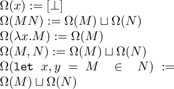 .
.
Figure 10: 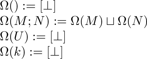 .
.
\[\begin{align} \Omega(\mathtt{meas}\;d\triangleright P\;\{0\to M\;|\;1\to N\})&:= \Omega(P)\sqcup \bigl([d\mapsto 0] \sqcup \Omega(M) \uplus [d\mapsto 1]\sqcup \Omega(N)\bigr) \\ \Omega(\mathtt{qcase}\;P\;\{0\to M\;|\;1\to N\}) &:= \Omega(P)\sqcup \Omega(M)\sqcup \Omega(N) \end{align}\] Therefore, elements of \(\Omega(M)\) are memory functions that provide exactly enough measurement outcomes to fully determine the term to which \(M\) will evaluate. In particular, we have \(\text{\textrm{Supp}}(\nu)\subseteq \text{Dev}(M)\) for all \(\nu\in\Omega(M)\). We further define the set of extended valuations of \(M\): \[\Omega_+(M):= \left\{\sigma\in\mathcal{M}\;\middle|\; \exists \nu\in\Omega(M):\nu\preceq \sigma \right\}.\] Then, given a well-formed configuration \(\vec{M}=\sum_i \alpha_i\cdot M_i^{\sigma_i}\in\vec{\mathscr{E}}\), the set of valuations of \(\vec{M}\) is defined as \[\Omega(\vec{M}) :=\bigcap_i \sigma_i \sqcup \Omega(M_i)\] Note that \(\sigma_i\) and elements of \(\Omega(M_i)\) have disjoint supports, guaranteeing that \(\Omega(\vec{M})\) is well defined.
5.2 Interpretation of Configurations↩︎
The goal of this section is to define an interpretation in \(\mathbf{CPM}\) of configurations of \(\vec{\mathscr{E}}\), which will be written as \(\llbracket \cdot \rrbracket\). The first step is to define an interpretation in \(\mathbf{FHilb}\) of terms \(M\in\mathscr{E}\), which is parametrized by a compatible valuation \(\nu\in \Omega_+(M)\). We will write this interpretation as \([\cdot]_\nu\). On types and typing contexts, \([\cdot]_\nu\) coincides with \([\cdot]\). For a typing judgment \(\Delta\vdash M:A\) with \(M\in\mathscr{E}\) and a valuation \(\nu\in\Omega_+(M)\), we inductively define the interpretation \([\Delta\vdash M:A]_\nu\). Compared to \([\cdot]\), the main addition is the rule for measurement, where the valuation is used to determine measurement outcomes: \[\scalebox{0.9}{ \begin{prooftree} \hypo{[\Delta \vdash P:\text{\textrm{q}}]_{\nu}\;= \;[\Delta] \xrightarrow{p} [\text{\textrm{q}}]} \hypo{[\Delta' \vdash M_i:A]_{\nu}\;= \;[\Delta']\xrightarrow{f_i}[A]} \hypo{\nu(d)=i} \infer3{[\Delta,\Delta'\vdash \mathtt{meas}\;d\triangleright P\;\{0\rightarrow M_0\;|\;1\rightarrow M_1\}: A]_\nu \;= \;[\Delta]\otimes[\Delta']\xrightarrow{p\otimes 1_{\llbracket \Delta' \rrbracket}} [\text{\textrm{q}}]\otimes [\Delta'] \xrightarrow{\mathfrak{m}_i(f_i)}[A]} \end{prooftree}}\] where \(\mathfrak{m}_i(f):= \bra{i}\otimes f\). For terms without measurement, the definition is similar to that of \([\cdot]\). The full definition is given in Appendix [sec:app:soundness].
lemmalemnuwelldefined For all valid typing judgment \(\Delta \vdash M:A\) where \(M\in\mathscr{E}\) and valuation \(\nu\in \Omega_+(M)\), \([\Delta\vdash M:A]_\nu\) is well defined.
We extend the definition to configurations as follows. Let \(\vec{M} = \sum_i \alpha_i\cdot M_i^{\sigma_i}\in\vec{\mathscr{E}}\) be a well-formed configuration for which there exist \(\Delta,A\) such that \(\Delta \vdash M_i: A\) is valid for all \(i\). Then, we define \[[\Delta;\vec{M};A]_{\nu}\;:=\;\sum_i \alpha_i[\Delta\vdash M_i:A]_{\nu}, \quad \text{for }\nu \in\Omega\bigl(\vec{M}\bigr).\] \([\cdot]_{\nu}\) is well defined—indeed, it is invariant with respect to congruence.
We can now introduce the interpretation of a configuration restricted to valuations compatible with a fixed memory function. Given a well-formed term \(\vec{M}\in \vec{\mathscr{E}}\), let \(\theta:\mathbb{D}\to\{0,1\}_\bot\) be a memory function such that \(\text{\textrm{Mem}}(\vec{M}) \;||\;\theta\). We define: \[\llbracket \Delta;\vec{M};A \rrbracket_{\theta} \;:=\;\sum_{ \nu\in\Omega(\vec{M}):\;\nu \;|| \;\theta} [\Delta;\vec{M};A]_\nu(\cdot)[\Delta;\vec{M};A]_\nu^\dagger\] In the particular case where \(\theta= [\bot]\), we omit the subscript and simply write \(\llbracket \Delta;\vec{M};A \rrbracket\). Then, \(\llbracket \cdot \rrbracket\) gives a semantics of the extended language in \(\mathbf{CPM}\). Generally, it does not yield morphisms of \(\mathbf{Caus}[\mathbf{CPM}]\). Nonetheless, we have the following property: the interpretation restricted to terms of \(\mathscr{E}\) coincides with the original definition on \(\mathscr{T}\), which justifies our using the same notation \(\llbracket \cdot \rrbracket\):
lemmalemcoincide Let \(M\in \mathscr{T}\) be a well-typed term. For appropriate \(\Delta\) and \(A\), we have: \[\llbracket \Delta \vdash M:A \rrbracket=\llbracket \Delta;\lceil M \rceil;A \rrbracket\]
5.3 Main Result↩︎
We now prove a soundness theorem stating that if one configuration can be reduced to another, then their denotations are the same.
theoremthmsoundness Let \(\vec{M}=\sum_i\alpha_i\cdot M_i^{\sigma_i}\) be a configuration for which \(\Delta \vdash M_i :A\) is valid for all \(i\), for some \(\Delta\) and \(A\). Consider a reduction \(\vec{M}\twoheadrightarrow \vec{M'}\). Then: \[\llbracket \Delta;\vec{M};A \rrbracket_{\text{\textrm{Mem}}(\vec{M})}=\llbracket \Delta;\vec{M'};A \rrbracket\]
A direct consequence is that if a configuration is reachable from a well-typed term of \(\mathscr{T}\) (via \(\lceil \cdot \rceil\) and \(\twoheadrightarrow\)), then it must be physically meaningful (see Remark 5). This implies by-design that no unitarity checks are needed to ensure physically in the operational semantics.
6 Expressivity↩︎
We study the expressivity of the language at first order and second order, i.e., at the level of quantum channels and of quantum supermaps, respectively.
We begin with first order. Recall that every quantum channel is a completely positive trace preserving map. We show that each quantum channel over qubits can be expressed by a term of the language:
propositionpropchannels Let \(\mathcal{C}\in \mathbf{CPM}(\mathbb{C}^{2^n},\mathbb{C}^{2^m})\) be a quantum channel from \(n\) qubits to \(m\) qubits. Then there exists a term \(M\) such that \(\vdash M : \text{\textrm{q}}^n \multimap\text{\textrm{q}}^m\) is derivable and \(\llbracket M \rrbracket = (1_{\llbracket \text{\textrm{q}}^n \rrbracket}\otimes \mathcal{C})\circ \eta'_{[\text{\textrm{q}}^n]}\).
The result on quantum channels is expected. Our main expressivity result concerns the level above, i.e. quantum supermaps. We show that the language implements a subclass of so-called quantum circuits with quantum control (QC-QCs), which we will refer to as QC-QCs with memory. Based on [4]’s definition of QC-QCs, we give the following definition. An \(N\)-linear map from \(\mathbf{CPM}(\mathcal{H}_I,\mathcal{H}_O)^N\) to \(\mathbf{CPM}(\mathcal{H}_P,\mathcal{H}_F)\) (where \(\mathcal{H}_I,\mathcal{H}_O,\mathcal{H}_P,\mathcal{H}_F\) are finite-dimensional Hilbert spaces) is said to be a QC-QC with memory if it is computed by a circuit of the following shape: \[\scalebox{0.9}{\tikzfig{qcqc}}\] For readability, we label a wire for Hilbert \(\mathcal{H}_X\) as \(X\). \(\mathcal{H}_{C_n}\) is defined as the finite-dimensional Hilbert space whose computational basis consists of the states \(\ket{(k_1,...,k_n)}\) where \(k_1,...,k_n\) are pairwise distinct elements of \(\{ 1,\ldots, N\}\). Each of the \(N\) open slots, which are given by variables \(x_{1},...,x_N\), is for one input channel. In this model, every open slot is controlled by a memory register (the bottom wire) that decides which input channel is plugged to which open slot. For instance, if the state of the control register of the left-most controlled open slot is \(\ket{(1)}\) then the first input channel \(x_1\) is applied, if the state is \(\ket{(2)}\) then the second channel \(x_2\) is applied, and if the state is \(\frac{\ket{(1)}+\ket{(2)}}{\sqrt 2}\), then \(x_1\) and \(x_2\) are applied in superposition.
The bottom register also plays the role of a memory: the \(n^\text{th}\) controlled open slot is controlled by a state of the form \(\ket{(k_1,...,k_n)}\), such that \(x_{k_1}, \ldots, x_{k_{n-1}}\) correspond to the input channels applied so far in this branch of the superposition, and \(x_{k_n}\) is the input channel which is plugged in the \(n^\text{th}\) open slot. Such a memory mechanism guarantees the linearity on the input channels: at the end of the circuit, for a given basis state of the memory register, each input channel has been applied once and only once. Indefinite causal order can thus be implemented when the state of memory register is in superposition. Each of these controlled open slot is intertwined with isometries \(V_{\ket{(k_1,...,k_n)}}^{\to k_{n+1}}\) that initialise and update the memory register in an appropriate way, depending on the higher order quantum operation one wants to implement.8
A more detailed presentation of QC-QCs with memory is given in Appendix [sec:app:QCQC].
We show that the language is universal for QC-QCs with memory:
propositionpropqcqc Let \(\mathcal{S}\) be a QC-QC with memory whose input consists of \(N\) channels in \(\mathbf{CPM}(\mathbb{C}^{2^n},\mathbb{C}^{2^m})\) and whose output is a channel in \(\mathbf{CPM}(\mathbb{C}^{2^k},\mathbb{C}^{2^l})\). Then there exists a term \(M\) of type \((\text{\textrm{q}}^n \multimap\text{\textrm{q}}^m)^{\otimes N}\multimap\text{\textrm{q}}^k \multimap\text{\textrm{q}}^l\) whose interpretation coincides with \(\mathcal{S}\).
The constructive, bottom-up approach of the definition directly gives us the implementation of a specific QC-QCs with memory. Therefore after defining a generalization of the \(\mathtt{qcase}\) construct to \(n\) branching statements, it is straightforward to construct a term that implements any QC-QC with memory. The construction is detailed in Appendix [sec:app:expressivity].
Remark 8. QC-QCs with memory are special instances of general QC-QCs. In the general case the bottom register stores which input channels have been applied so far but not in which order (the basis states of this register are then sets rather than lists). We leave for further development the implementation of general QC-QCs.
7 An Extension for Non-Linearity and Recursion↩︎
We have defined a linear programming language which supports both measurements and processes with indefinite causal orders. Although linearity is the key feature that enables us combine these two features, requiring all programs to be strictly linear is a considerable restriction. Indeed, we cannot implement any quantum algorithm whose input is an oracle that is queried more than once. To address this limitation, we define an extension of the language that includes some nonlinear features, and give its operational semantics. Notably, this extension has a \(\mathtt{letrec}\) construct for recursive processes, because multiple calls to a function are now allowed.
7.1 Syntax and Type System↩︎
The extension of the syntax is fairly straightforward: we add nonlinear versions of the terms of the lambda calculus, and terms for recursion. In addition to the set \(\mathcal{X}\) of linear variables, we define a countably infinite set \(\mathcal{V}\) of duplicable variables, written as \(u,v,w...\). The set of terms \(\mathscr{T}^*\supseteq \mathscr{T}\) is defined by the grammar in Figure 11.
None
Figure 11: Extended syntax.
The terms \(u,M^*N,\lambda^*u.M\) denote nonlinear variables, application and \(\lambda\)-abstraction. Whereas the term \(M\) in \(\lambda x. M\) must contain exactly one occurrence of \(x\) (counting occurrences in different branches of \(\mathtt{meas}\) or \(\mathtt{qcase}\) as the same), the term \(M\) in \(\lambda^* u. M\) must contain at least one occurrence of \(u\). The term \(\mathtt{letrec}\;f\;x=M\) recursively defines \(f\) as a linear function of \(x\); the term \(\mathtt{letrec}^*\;f\;u=M\) recursively defines \(f\) as a nonlinear function of \(u\). In both cases, the function symbol \(f\) itself is a duplicable variable.
We define a set of controllable terms \(\mathscr{C}^*\subseteq \mathscr{T}^*\) as the set of terms that do not contain duplicable variables or measurement.
The type system is extended to include a nonlinear function type \(\Rightarrow\): \[\begin{array}{lll} \text{(Extended types)}\quad A,B \;& ::= \;& \text{\boldsymbol{1}}\;|\;\text{\textrm{q}}\;|\; A \otimes B \;|\;A \multimap B \;|\;A \Rightarrow B \end{array}\] We now distinguish linear and unrestricted typing contexts. A linear typing context is a list \(\Delta = x_1:A_1,...,x_n:A_n\) where \(x_1,...,x_n\) are pairwise distinct linear variables and \(A_1,...,A_n\) their respective types. An unrestricted typing context is a list \(\Gamma = u_1:A_1,...,u_n:A_n\) where \(u_1,...,u_n\) are pairwise distinct duplicable variables and \(A_1,...,A_n\) their respective types. Then, typing judgments are expressions of the form \[\Gamma; \Delta \vdash M :A\] where \(M\) is a term, \(A\) a type, \(\Gamma\) an unrestricted typing context and \(\Delta\) a linear typing context. The typing rules are obtained by extending the linear type system in the expected way.9
7.2 Operational Semantics↩︎
The main difficulty of the operational semantics is keeping track of which measurement outcomes must be synchronized. In the linear fragment, this is achieved by assigning to each measurement a unique device reference \(d\) and recording its outcome via a memory function.
However, the possible duplication of terms in the nonlinear extension invalidates the device reference approach. To see this, consider the execution term \(\texttt{Meas}[d]\) of Section 3.1 On the one hand, by reducing the term \[\label{eq:linear95duplication} (\lambda y. \mathtt{qcase}\;H\ket{0} \;\{0\to y\;|\;1\to y\})\; \texttt{Meas}[d],\tag{2}\] we will obtain two copies of \(\texttt{Meas}[d]\), whose measurement outcomes must be synchronized. But on the other hand, the term \[(\lambda^*u. \pair{u\ket{0},u\ket{1}})\;\texttt{Meas}[d]\] should be read as creating two independent occurences of the process \(\texttt{Meas}[d]\), which are then applied to distinct inputs. This is essentially the same as creating a second measurement device; their measurement outcomes should therefore also be independent.
To resolve this issue, we modify the treatment of device references so that nonlinearity can be interpreted as duplicating the devices themselves. We define the set of extended device references \(\mathbb{D}^*\) as sequences \(d\cdot n_1 \cdot ...\cdot n_k\) where \(d\in\mathbb{D}\) is a device reference, \(k\geq 0\) and \(n_1,...,n_k\geq 1\). In particular, \(\mathbb{D}\subseteq \mathbb{D}^*\). Then, an extended memory function is a function from \(\mathbb{D}^*\) to \(\{0,1\}_\bot\) such that only a finite number of elements of \(\mathbb{D}\) are mapped to \(\{0,1\}\).
In order to define the operational semantics, we define execution terms and terms superpositions similarly to the linear language, replacing device references and memory functions with their extended counterparts. A more detailed explanation is provided in Appendix [sec:app:extension95op]. For all pair of execution terms \(M,N\) and \(u\in\mathcal{V}\), \(M\{\mskip-5mu\{ N/u \}\mskip-5mu\}\) is defined as the execution term where the \(n\)-th occurrence of \(u\) in \(M\) is replaced by \(N\) in which every extended device reference \(d^*\) is replaced by \(d^* \cdot n\). For example: \[\begin{align} &\pair{\lambda x. M\,u,u}\{\mskip-5mu\{ \mathtt{meas}\;d^*\triangleright H\ket{0}\; \{0\to \ket{0} \;|\;1\to \ket{1}\}/u \}\mskip-5mu\}\\ &\quad := \pair{\lambda x. M\,\mathtt{meas}\;(d^*\cdot 1) \triangleright H\ket{0}\;\{0\to \ket{0} \;|\;1\to \ket{1}\},\mathtt{meas}\;(d^*\cdot 2)\triangleright H\ket{0}\;\{0\to \ket{0} \;|\;1\to \ket{1}\}}\; \end{align}\]
Therefore, we can extend the reduction relation \(\twoheadrightarrow\), where the main novelty is the rules for nonlinear abstraction and recursion (the full definition is given in Appendix [sec:app:extension95op]) : \[\scalebox{1}{ \begin{prooftree} \infer0{(\lambda^* u. M)^*V\twoheadrightarrow M\{\mskip-5mu\{ V/u \}\mskip-5mu\}} \end{prooftree}} \qquad \scalebox{1}{ \begin{prooftree} \infer0{(\mathtt{letrec}\;f\;x=M )V \twoheadrightarrow M\{V/x\}\{\mskip-5mu\{ \mathtt{letrec}\;f\;x=M/f \}\mskip-5mu\}} \end{prooftree}}\] \[\scalebox{1}{ \begin{prooftree} \infer0{(\mathtt{letrec}^*\;f\;u=M)^*V \twoheadrightarrow M\{\mskip-5mu\{ V/u \}\mskip-5mu\}\{\mskip-5mu\{ \mathtt{letrec}^* \;f\;u=M/f \}\mskip-5mu\}} \end{prooftree}}\]
Lastly, we can check that the standard properties of the typing and operational semantics (substitution—Lemma [lem:substitution], subject reduction—Proposition [prop:subject95reduction], progress—Lemma [lem:progress] and uniqueness of the normal form—Proposition [prop:confluence]) still hold.
7.3 Examples↩︎
Example 8 (No-cloning). Due to the linear evaluation strategy, the term \(\lambda^*u.\pair{u,u}\) acts by copying a qubit along the computational basis, not cloning it. To illustrate this, suppose the term is applied to \(U\ket{0}\), which we assume reduces to \(\alpha\ket{0}+\beta\ket{1}\): \[\begin{align} (\lambda^*u.\pair{u,u} )(U\ket{0}) & \twoheadrightarrow \alpha \cdot (\lambda^*u.\pair{u,u} )\ket{0} +\beta\cdot (\lambda^*u.\pair{u,u} )\ket{1} \\ & \twoheadrightarrow \alpha \cdot \ket{0,0} +\beta\cdot (\lambda^*u.\pair{u,u} )\ket{1} \twoheadrightarrow \alpha\cdot \ket{0,0} +\beta \cdot\ket{1,1} \end{align}\] In contrast, cloning would have given the following result: \[\begin{align} \pair{U\ket{0},U\ket{0}}&\twoheadrightarrow \alpha\cdot \pair{U\ket{0},\ket{0}}+\beta\cdot \pair{U\ket{0},\ket{1}} \twoheadrightarrow \alpha^2\cdot \ket{0,0}+\alpha\beta\cdot \ket{1,0}+\beta\alpha \cdot\ket{0,1} + \beta^2\cdot\ket{1,1} \end{align}\]
Example 9 (Repeat-Until-Success). In [25], the authors define “Repeat-Until-Success” circuits, which are non-deterministic circuits that minimize the \(T\) count required to approximate single-qubit unitary gates. Repeat-Until-Success circuits can be implemented in our language by recursive terms of the following form: \[\begin{align} \mathtt{letrec}\;f \;z = \;& \mathtt{let}\;\pair{x,y}= \mathtt{U}\;\pair{\ket{0},z} \;\mathtt{in} \;\mathtt{meas}\;x \;\{0\to \pair{y,f} \;|\;1\;\to f\,y\} \end{align}\] where \(\mathtt{U}\) is a term of type \(\text{\textrm{q}}\otimes\text{\textrm{q}}\multimap\text{\textrm{q}}\otimes \text{\textrm{q}}\) implementing a 2-qubit unitary gate. The program returns a pair consisting of the output qubit together with a copy of the recursive function \(f\).
This work is supported by the the Plan France 2030 through the PEPR integrated project EPiQ ANR-22-PETQ-0007 and the HQI platform ANR-22-PNCQ-0002; and by the European projects Quantum Flagship NEASQC, European MSCA Staff Exchanges Qcomical HORIZON-MSCA-2023-SE-01. The project is also supported by the Maison du Quantique MaQuEst.
References↩︎
To define the reduction of this term, we will see in Section 3 that the operational semantics relies on a set of execution terms whose typing is slightly more permissive.↩︎
The notion of “physically meaningful” will be clarified in Section 4.↩︎
The step-by-step sequence of reductions is detailed in Appendix [sec:app:example95switch].↩︎
See details in Appendix [sec:app:meas95transfer].↩︎
Specifically the variant given in [52], [53] which explicitly uses dual vector spaces.↩︎
\(\lambda,\mu\) being invertible means that \(\lambda,\mu\) are isomorphisms; \(\lambda \mathfrak{d}_A\) and \(\mu \mathfrak{d}^*_A\) should be read as \(\lambda \otimes \mathfrak{d}_A\) and \(\mu \otimes \mathfrak{d}^*_A\).↩︎
Note that the \(\mathcal{P}_k\) are not morphisms of \(\mathbf{Caus}[\mathbf{CPM}]\).↩︎
Additionally, the output spaces of the \(V_{\ket{(k_1,...,k_N)}}^{\to F}\) are assumed to be orthogonal.↩︎
See Appendix [sec:app:extension95typing].↩︎