How Does Bayesian Causal Discovery Fail?
Characterising Structural Consequences in Linear Gaussian Networks under Latent Confounding
July 10, 2026
Abstract
Bayesian causal discovery is widely used for its ability to quantify epistemic uncertainty over directed acyclic graphs (DAGs) through posterior inference. However, its behaviour under latent confounding remains poorly understood, as existing work typically notes that confounding breaks identifiability without characterising how the posterior distribution over DAGs responds. In this work, we analyse posterior behaviour under latent confounding in linear Gaussian causal models, focusing on additive latent confounding between exactly two observed variables. We derive a critical correlation threshold above which the score function favours graphs with a spurious edge between the confounded variables, and show that this threshold decreases with sample size – more data lowers the correlation required for the spurious edge to be favoured. Beyond this threshold, we characterize two distinct posterior failure regimes determined by the local structure around the confounded variables. Our findings are supported by exact posterior computations on multiple graph structures, demonstrating both the predicted failure regimes.
1 Introduction↩︎
Discovering the causal relationships underlying a system of variables is a central problem across scientific domains. Bayesian networks and structural equation models provide a principled framework for representing such dependencies [1], [2]. Structure learning methods aim to recover a graph representing the underlying data generating process from observational data, but are inherently limited by statistical uncertainty and identifiability constraints [3]. In contrast, Bayesian causal structure learning infers a posterior distribution \(p(G \mid D)\) over candidate directed acyclic graphs (DAGs) representing the underlying causal system [4], enabling principled quantification of epistemic uncertainty. This distribution allows assessing confidence in inferred structures and supports downstream tasks such as experimental design and active causal discovery [5], [6], where uncertainty over candidate graphs plays a central role. However, how this posterior uncertainty changes under violations of modelling assumptions, such as latent confounding, is not well understood.
The reliability of posterior-based causal conclusions from observational data—namely, whether posterior probabilities faithfully reflect uncertainty over plausible structures—depends on two key components: identifiability and scoring. On the identifiability side, under the assumptions of the causal Markov condition, causal sufficiency (lack of latent confounding), and faithfulness, observational data can distinguish causal structures only up to Markov equivalence [7], [8], even under infinite data. On the scoring side, the choice of score—such as the Bayesian Gaussian equivalent (BGe) score in linear Gaussian models [9], [10]—determines the likelihood and prior that govern how evidence is translated into posterior probabilities over candidate causal structures, under assumptions such as independent exogenous noise and Gaussianity. While both identifiability and scoring are well understood under standard assumptions, it remains unclear how their interplay affects posterior behaviour when these assumptions are violated.
Of these assumptions, causal sufficiency is particularly consequential for causal discovery from observational data. The assumption is not testable in practice, yet it is routinely violated in many applications. Causal discovery methods are widely applied to settings such as gene regulatory network inference from expression data [11]–[13]. Here, unmeasured cell states, batch effects, and latent regulatory factors can induce confounding effects [14]–[16]. Similarly, in clinical epidemiology, Bayesian structure learning is used on observational patient data where unmeasured characteristics are a recognised source of confounding bias [17]. For Bayesian causal discovery, these practical violations raise the question of how posterior uncertainty behaves under latent confounding.
Existing work on Bayesian causal discovery and latent confounding falls into two main categories. (i) A substantial line of work develops Bayesian inference over DAGs under the assumption of causal sufficiency—including order MCMC [4] and GADGET [18]. (ii) A parallel line addresses confounding by switching to richer model classes, motivated by the fact that in the presence of latent confounders the causal structure over observed variables is generally not identifiable as a causally sufficient DAG from observational data [19], [20]. This includes constraint-based methods such as FCI and its variants [19], [21], which return partial ancestral graphs, and Bayesian inference jointly over acyclic directed mixed graphs (ADMGs) and latent variables [22]—solving the problem by changing the inference target. Empirical benchmarks under assumption violations further show that most benchmarked causal discovery methods do not explicitly support confounding effects, and that spurious correlations induced by latent confounding degrade edge selection and graph recovery [23]. None of these approaches address the critical question of what happens when Bayesian causal discovery methods operating on DAGs are applied to data with unobserved confounding: whether the posterior appropriately reflects the resulting uncertainty, or instead concentrates on systematically incorrect inferred structures. More broadly, is this behaviour structured and predictable, or inherently unreliable?
In this paper, we address the above question by providing a structural characterisation of posterior behaviour under latent confounding. We consider a simple but representative setting of a single additive latent confounder affecting exactly two observed variables in linear Gaussian models with additive noise. Within this setting, we derive a sample-size-dependent critical correlation threshold, beyond which the posterior begins to shift towards incorrect causal graphs. We then identify two qualitatively distinct failure regimes in which posterior behaviour is governed by the structural properties of the local region affected by confounding.
2 Background↩︎
2.1 Linear Gaussian SCMs and Latent Confounding↩︎
A structural causal model (SCM) over variables \(\mathbf{X} = (X_1, \dots, X_n)\) specifies each variable as a deterministic function of its causal parents and an independent exogenous noise term [1]. We work with linear Gaussian SCMs, in which each variable follows \[X_i = \sum_{j \in \mathrm{pa}(i)} \beta_{ij} X_j + \varepsilon_i, \qquad \varepsilon_i \sim \mathcal{N}(0, \sigma_i^2),\] where \(\mathrm{pa}(i)\) is the parent set of \(X_i\) in a directed acyclic graph (DAG) \(G\), the noise terms \(\varepsilon_i\) are mutually independent, and the coefficients \(\beta_{ij}\) are bounded away from zero to ensure non-trivial dependence along each edge. The DAG, coefficients, and noise variances jointly induce a centered Gaussian distribution over \(\mathbf{X}\).
The setting above assumes that every common cause of any pair of observable variables is itself observable. When this fails, an unobserved variable \(H\) may influence multiple observable variables simultaneously. We adopt a Gaussian additive latent confounder model: if \(H \sim \mathcal{N}(0, \sigma_H^2)\) confounds two observable variables \(X_j\) and \(X_k\) that are non-adjacent in the underlying DAG, their structural equations become \[X_j = \sum_{\ell \in \mathrm{pa}(j)} \beta_{j\ell} X_\ell + \gamma_j H + \varepsilon_j, \quad X_k = \sum_{\ell \in \mathrm{pa}(k)} \beta_{k\ell} X_\ell + \gamma_k H + \varepsilon_k, \label{eq:confounder}\tag{1}\] with confounding coefficients \(\gamma_j, \gamma_k\) and noise terms independent of \(H\). We choose \(H\) Gaussian so that the joint distribution over \(\mathbf{X}\) remains Gaussian after marginalising \(H\). Marginalisation introduces an additional covariance contribution \(\gamma_j \gamma_k \sigma_H^2\) between \(X_j\) and \(X_k\): since \(X_j\) and \(X_k\) are not connected by an edge, no DAG representing the observable causal structure can account for this dependence.
2.2 Bayesian Network Structure Learning↩︎
A Bayesian network represents the dependencies among variables \(X_1, \dots, X_n\) through a directed acyclic graph (DAG) \(G\), in which each variable is conditionally independent of its non-descendants given its parents \(\mathrm{pa}_G(i)\) [1]. The joint distribution factorises as \[p(X_1, \dots, X_n \mid G) = \prod_{i=1}^n p\bigl(X_i \mid \mathrm{pa}_G(i)\bigr), \label{eq:factorisation}\tag{2}\] and different DAGs encode different sets of conditional independence relations.
The goal of Bayesian structure learning is to infer the DAG from data. Since different DAGs impose different conditional independence relations and therefore different factorisations of the joint distribution, the marginal likelihood \(P(\mathcal{D} \mid G)\) of the observed data depends on the specific DAG \(G\). We assume the dataset consists of \(N\) observations \(\mathcal{D} = \{\mathbf{x}^{(1)}, \dots, \mathbf{x}^{(N)}\}\), where each \(\mathbf{x}^{(j)} \in \mathbb{R}^n\) is a realisation of the random vector \(\mathbf{X} = (X_1, \dots, X_n)^\top\). Following the Bayesian paradigm [4], the posterior over DAGs is \[P(G \mid \mathcal{D}) \;=\; \frac{P(\mathcal{D} \mid G)\, P(G)}{P(\mathcal{D})} \;\propto\; P(\mathcal{D} \mid G)\, P(G), \label{eq:posterior}\tag{3}\] where \(P(G)\) is the prior over DAGs and \(P(\mathcal{D}) = \sum_{G'} P(\mathcal{D} \mid G')\, P(G')\) is a normalising constant independent of \(G\). In the absence of prior knowledge over graphs, we assume all DAGs to be equally likely a priori, \(P(G) = c\) for all \(G\), so the posterior is proportional to the marginal likelihood.
The marginal likelihood is obtained by integrating out the local parameters \(\theta\)—the edge coefficients \(\{\beta_{ij}\}\) and noise variances \(\{\sigma_i^2\}\) defining the conditional distributions of each node given its parents—against a parameter prior: \[P(\mathcal{D} \mid G) \;=\; \int P(\mathcal{D} \mid G, \theta)\, P(\theta \mid G)\, d\theta.\]
Two DAGs are Markov equivalent if they imply the same conditional independence relations among \(X_1, \dots, X_n\); observational data alone cannot distinguish between them [7], [24]. By definition, two DAGs are Markov equivalent if and only if they share the same skeleton (the undirected graph obtained by ignoring edge directions) and the same set of colliders: triples \(X_i \to X_j \leftarrow X_k\) in which \(X_i\) and \(X_k\) are not adjacent. The resulting equivalence classes are called Markov equivalence classes (MECs). A marginal likelihood is score-equivalent if it assigns identical values to all DAGs within an MEC, since these DAGs are observationally indistinguishable. There exist only two Bayesian scores that satisfy this property: the discrete BDe score for categorical data and the Gaussian BGe score for linear Gaussian SCMs [25]. We focus on the BGe score throughout this work.
For linear Gaussian SCMs, the joint distribution of \(\mathbf{X}\) under a DAG \(G\) is multivariate Gaussian, \(\mathbf{X} \mid G \sim \mathcal{N}_n(\boldsymbol{\mu}^G, \Sigma^G)\), with mean vector \(\boldsymbol{\mu}^G\) and covariance \(\Sigma^G\) chosen to be coherent with the factorisation 2 implied by \(G\). The BGe score [9] places a fully conjugate normal–Wishart prior on the joint mean and precision \((\boldsymbol{\mu},\Sigma^{-1})\), \[\boldsymbol{\mu} \mid \Sigma \sim \mathcal{N}_n\bigl(\boldsymbol{\mu}_0, \alpha_\mu^{-1} \Sigma\bigr), \qquad \Sigma^{-1} \sim \mathcal{W}_n(\alpha_w, T),\] parameterised by a prior mean \(\boldsymbol{\mu}_0 \in \mathbb{R}^n\), prior precision \(\alpha_\mu > 0\) on the mean, prior degrees of freedom \(\alpha_w > n - 1\), and positive-definite scale matrix \(T \in \mathbb{R}^{n \times n}\). Here, \(\mathcal{W}_n(\alpha_w, T)\) denotes the \(n\)-dimensional Wishart distribution. Conjugacy with the Gaussian likelihood yields a normal–Wishart posterior, and the marginal likelihood \(P(\mathcal{D} \mid G)\) of G can be computed analytically and is called the BGe score of G. Due to modularity property of the score, the log of the score decomposes into a sum of local scores: \[s(G) := \log P(\mathcal{D} \mid G) = \log \prod_{i=1}^{n} P\bigl(\mathcal{D} \mid i, \operatorname{pa}_G(i)\bigr) = \sum_{i=1}^{n} s\bigl(i, \operatorname{pa}_G(i)\bigr). \label{eq:decomp}\tag{4}\] Since the logarithm is monotonic and we use a uniform prior over graphs, comparisons of \(s(G)\) values are equivalent to comparisons of the scores; we therefore work with \(s(G)\) throughout. A more detailed exposition of the BGe score can be found in [9], [10].
3 Spurious Edge Inclusion under Latent Confounding↩︎
The latent confounder \(H\) in Equation 1 induces an additional dependence between \(X_j\) and \(X_k\). Once this dependence is strong enough, it cannot be explained by any directed edge among the observed variables. Consequently, the marginal likelihood \(P(\mathcal{D} \mid G)\) in Bayesian structure learning favours DAGs that include a directed edge \(X_k \to X_j\) (or its reverse) to account for this correlation. We call this induced edge as spurious edge in the context of causality as it represents an incorrect causal link.
In this section, we quantify how strong this confounding induced correlation must be for DAGs with such an edge to be favoured by the marginal likelihood. We begin by deriving a critical correlation threshold based on the partial correlation induced by the confounder. We then show that asymmetry in the parent sets makes one direction of an edge strictly easier to be induced than the other.
3.1 Critical Threshold for Spurious Edge Inclusion↩︎
The key to our analysis is that comparing two DAGs that differ only in a single edge reduces to a local computation. Latent confounding induces an excess dependence between the confounded variables that the true graph cannot explain; the relevant question is whether the score favours adding a direct edge between them to absorb this dependence. We therefore compare the graph without this edge against the one with it, and ask when the latter is preferred. Recall that the log of the BGe score is given by Equation 4 .
Let \(G = (V, E)\) be the underlying causal graph over variables \(\{X_1, \dots, X_n\}\), with latent confounding between \(X_k\) and \(X_j\). Consider two DAGs \(G\) and \(G'\) that are identical except that \(G'\) contains the additional edge \(X_k \to X_j\), i.e., \(\operatorname{pa}_{G'}(j) = \operatorname{pa}_G(j) \cup \{k\}\), while all other parent sets are unchanged. By decomposability in 4 , every node-wise term is identical in the two graphs except that of \(X_j\), so their score difference reduces to a single local term: \[s(G') - s(G) = s(j, \operatorname{pa}_G(j) \cup \{k\}) - s(j, \operatorname{pa}_G(j)).\] The score favours including the edge precisely when this difference is positive. Deciding whether to include \(X_k\) as a parent of \(X_j\) therefore reduces to a local score comparison involving only node \(j\), its current parents \(P := \operatorname{pa}_G(j)\), and the candidate parent \(k\) – independent of the rest of the graph. The following proposition formalises this local score comparison, expressing it in terms of the partial correlation induced between \(X_j\) and \(X_k\) given \(P\) given by \(\rho_{jk \mid P}\) and identifying the critical value at which the score begins to favour the additional edge. See Appendix 7 for a detailed derivation.
Proposition 1 (Critical correlation threshold). Assume a regular linear Gaussian data-generating process on a causal graph \(G = (V, E)\) over variables \(\{X_1, \dots, X_n\}\), with latent confounding between \(X_k\) and \(X_j\). Let \(P = \operatorname{pa}_G(j)\) be the current parent set of \(X_j\), and let \(G'\) denote the graph obtained from \(G\) by adding the edge \(X_k \to X_j\) (i.e., \(\operatorname{pa}_{G'}(j) = P \cup \{k\}\), with all other parent sets unchanged). Then, for sufficiently large sample size \(N\) and fixed BGe hyperparameters, the BGe score prefers \(G'\) over \(G\) whenever the partial correlation \(\rho_{jk \mid P}\) exceeds a critical value \(\rho_c\); that is, when \[N \log\!\left(\frac{1}{1-\rho_{jk \mid P}^2}\right) > \log N .\] The critical partial correlation \(\rho_c\) is defined by the equality \[N \log\!\left(\frac{1}{1-\rho_c^2}\right) = \log N ,\qquad\text{i.e.}\qquad \rho_c^2 = 1 - N^{-1/N}.\] so that the score favours the additional edge whenever \(\rho_{jk \mid P} > \rho_c\).
Remark 2. The threshold condition has the closed-form solution \(\rho_c^2 = 1 - e^{-\log N / N}\). For large \(N\), expanding the exponential gives \[\rho_c \approx \sqrt{\frac{\log N}{N}}.\] The graph-independent critical partial correlation therefore decreases with sample size: more data lowers the correlation required to favour the edge, so weaker correlation \(\rho_{jk \mid P}\) caused by confounding suffices to induce the spurious edge.
3.2 Asymmetry and the Preferred Direction↩︎
The above analysis considered adding \(X_k\) as a parent of \(X_j\), conditioning on the set of observed parents \(P\) of \(X_j\). Without prior causal knowledge, the reverse orientation \(X_j \to X_k\) is also a candidate and the two compete score-wise. We show by an example that the asymmetry of parent sets causes DAGs with a particular orientation of the spurious edge to be preferred over the DAGs with the reverse orientation of the same edge.
Consider the small SCM in Figure 1, where \(X_j\) has the observed parents set \(P = \{ X_{p_1}, X_{p_2} \}\) . Let \(X_P = (X_{p_1}, X_{p_2})\) with coefficient vector \(\beta_P\), \(X_k\) have no observed parents, and the latent variable \(H\) confounds the pair: \[H \sim \mathcal{N}(0, \sigma_H^2), \quad X_k = \gamma_k H + \varepsilon_k, \quad X_j = \beta_P^\top X_P + \gamma_j H + \varepsilon_j,\] with mutually independent Gaussian noise terms \(\varepsilon_j \sim \mathcal{N}(0, \sigma_j^2)\) and \(\varepsilon_k \sim \mathcal{N}(0, \sigma_k^2)\), independent of \(H\).
The partial correlations for including the two candidate edges given the remaining graph stays the same are: \[\rho_{jk \mid P} = \frac{\gamma_j \gamma_k \sigma_H^2}{\sqrt{(\gamma_j^2 \sigma_H^2 + \sigma_j^2)(\gamma_k^2 \sigma_H^2 + \sigma_k^2)}},\] \[\rho_{kj \mid \varnothing} = \frac{\gamma_j \gamma_k \sigma_H^2}{\sqrt{(\gamma_j^2 \sigma_H^2 + \sigma_j^2 + \beta_P^\top \Sigma_P \beta_P)(\gamma_k^2 \sigma_H^2 + \sigma_k^2)}},\] where \(\beta_P^\top \Sigma_P \beta_P = \operatorname{Var}(\beta_P^\top X_P)\) is the variance of \(X_j\) explained by its observed parents. The two expressions share the same numerator; the reverse edge’s denominator carries the extra \(\beta_P^\top \Sigma_P \beta_P\) term because the reverse direction conditions on no parents. Hence \(\rho_{jk \mid P} > \rho_{kj \mid \varnothing}\). So, whenever the reverse partial correlation exceeds the critical threshold \(\rho_c\), the forward one does too (by Proposition 1); the converse is not generally true. In the regime where both correlations exceed \(\rho_c\) and both candidate DAGs score higher than \(G\), the choice between them reduces to a direct comparison of their local terms: \[s(G \cup \{X_k \to X_j\}) - s(G \cup \{X_j \to X_k\}) \approx \frac{N}{2}\left[ \log\!\left(\frac{1}{1-\rho_{jk \mid P}^2}\right) - \log\!\left(\frac{1}{1-\rho_{kj \mid \varnothing}^2}\right) \right] > 0,\] so \(G \cup \{X_k \to X_j\}\) is strictly preferred. This asymmetry implies that, when a latent confounder induces a spurious edge, the score favours the orientation directed towards the confounded variable with parents in the underlying causal graph over the orientation directed towards the one without. More generally, the preferred orientation points to the variable whose parents explain more of its variance: conditioning on these parents reduces the residual variance and raises the induced partial correlation, leading to DAGs with this orientation having a higher score than the one with opposite orientation.

4 Posterior Behaviour Beyond Critical Correlation↩︎
We now examine how Bayesian causal discovery behaves when the partial correlation induced by confounding exceeds the threshold established in Section 3.1: does the posterior concentrate on DAGs that contain only a spurious edge between the confounded nodes while preserving the correct causal relations among non-confounded variables, or on DAGs that also corrupt those relations that were recovered correctly in the unconfounded setting. Throughout this section, “latent confounding” refers to the case when the partial correlation between the confounded variables induced by confounding is beyond the critical threshold of Section 3.1.
4.1 Markov Equivalence and Posterior Connection↩︎
We now illustrate, through simple graphs, that posterior preference for DAGs over others is governed not only by the BGe score, but also by the dynamics of the collider structures in the highest scoring DAGs.
Consider a chain \(X_1 \to X_2 \to X_3\) as the underlying causal graph. It is Markov equivalent to the reverse chain \(X_1 \leftarrow X_2 \leftarrow X_3\) and the fork \(X_1 \leftarrow X_2 \to X_3\) (where \(X_2\) is the fork node, the common cause of \(X_1\) and \(X_3\)). These three DAGs are observationally indistinguishable, and since the BGe score is score-equivalent within a MEC [9], Bayesian structure learning assigns them equal posterior mass. The posterior probability of a directed edge is the total mass of the DAGs containing it; the true edges \(X_1 \to X_2\) and \(X_2 \to X_3\) receive only one-third and two-thirds of the posterior mass, respectively.
In contrast, the collider \(X_1 \to X_2 \leftarrow X_3\) is uniquely identifiable from observational data, since it induces a distinct conditional independence pattern. Its MEC contains only a single DAG, so the true edges are learned with high confidence. Now suppose \(X_1\) and \(X_3\) are latently confounded. The score favours DAGs containing an edge between \(X_1\) and \(X_3\) to explain the induced correlation. Once this edge is present, the collider at \(X_2\) is destroyed, and no new collider can form anywhere among the three nodes since all three pairs of nodes are now adjacent. Consequently, every orientation of the resulting fully connected three-node DAG, shown in Figure 2 (a), is Markov equivalent and receives the same score. Posterior mass therefore distributes across all six equivalent DAGs in its MEC, and the true edges \(X_1 \to X_2\) and \(X_3 \to X_2\) receive substantially lower posterior probability than in the unconfounded setting – reducing confidence in their detection.
Now consider the true causal graph shown in Figure 2 (b). With no confounding, all DAGs Markov equivalent to it have the highest score, and since the MEC contains two DAGs, shown in Figure 2 (b) and Figure 2 (c), the probability is distributed equally between the edges \(X_1 \to X_4\) and \(X_4 \to X_1\). Under confounding between \(X_1\) and \(X_3\), the DAG in Figure 2 (d) receives the highest score among all other DAGs due to parent asymmetry discussed in Section 3.2. However, in this case, though the collider at \(X_2\) is destroyed, \(X_4 \to X_1 \leftarrow X_3\) forms a new collider at \(X_1\). The MEC now only contains this single graph and, hence the posterior probability of the true causal edge \(X_4 \to X_1\) increases compared to the unconfounded setting.

These examples demonstrate that size of the MEC of the highest scoring DAGs determines the probability of recovering true edge directions. Importantly, colliders are the essential graphical objects: their formation or destruction directly changes the MEC of the graph, and consequently governs whether the posterior remains concentrated or spreads across multiple competing structures.
4.2 Structural Characterization and Failure Regimes↩︎
Consider a true causal DAG \(G=(V,E)\) over observed variables \(\{X_1,\dots,X_n\}\), and suppose latent confounding is introduced between variables \(X_j\) and \(X_k\), where \((X_j, X_k) \notin E\). In the absence of confounding, the highest-scoring structures are \(G\) and the DAGs Markov equivalent to it, and posterior mass concentrates on this MEC. The posterior probabilities of edges are determined by the frequency with which those edges appear across these DAGs.
Under latent confounding, the covariance structure generated by the original causal relations remains present in the data, so the true causal directions continue to receive strong scores. However, the additional dependence induced between \(X_j\) and \(X_k\) is not explained by \(G\). Consequently, Bayesian structure learning assigns higher scores to structures that additionally contain a spurious edge between the confounded variables. The highest-scoring structures are therefore \(G\) augmented with one of the two orientations of this edge, together with their Markov equivalents: \[G \cup \{X_j \to X_k\} \qquad\text{or}\qquad G \cup \{X_k \to X_j\},\] and the DAGs Markov equivalent to each.
When both orientations satisfy acyclicity constraints, two factors combine to determine the dominant orientation. First, one orientation may achieve a higher score due to structural asymmetries such as differing parent sets. Second, a smaller MEC concentrates posterior mass on fewer DAGs. When both effects favour the same orientation it dominates decisively; when they conflict, the outcome depends on whether the score advantage outweighs the difference in MEC size.
Although MECs are properties of the full graph, latent confounding modifies the observational structure only through the confounded variables and their adjacent edges. We define the confounded region as the local subgraph of the DAG \(G\) induced by the confounded nodes together with their immediate neighbouring nodes in the underlying true causal graph. This does not contain the spurious edge. Consequently, relative to the unconfounded setting, changes in the MEC arise from local changes in the confounded region. The remaining graph preserves the same equivalence relations as before confounding, making the local confounded structure sufficient for characterizing the resulting posterior behaviour even in larger graphs.
Since MECs are determined by the skeleton and colliders, the key structural mechanism is whether the spurious edge preserves, creates, or weakens collider-based orientation constraints within the confounded region. This yields the following structural characterisation of the posterior behaviour, depending on whether the confounded region initially contains colliders. In what follows, ‘number of colliders’ refers to the number of distinct collider nodes, i.e. nodes with two or more non-adjacent parents.
4.2.0.1 Case 1: Confounded region contains colliders.
At least one orientation of the spurious edge preserves or increases the number of colliders in the confounded region. For e.g. in Figure 2 (b) with confounding between \(X_1\), \(X_3\).
Both orientations of the spurious edge reduce the number of colliders in the confounded region. For e.g the collider \(X_1 \to X_2 \leftarrow X_3\) with confounding between \(X_1\), \(X_3\).
4.2.0.2 Case 2: Confounded region contains no colliders.
At least one orientation of the spurious edge creates new colliders in the confounded region. For e.g. the chain \(X_1 \to X_2 \to X_3 \to X_4\) with confounding between \(X_1\), \(X_4\).
Neither orientation of the spurious edge creates colliders in the confounded region. For e.g. \(X_1 \leftarrow X_2 \to X_3\) with confounding between \(X_1\), \(X_3\).
These structural cases now induce two qualitatively different failure regimes, where “failure” refers to the inference of a confounding-induced incorrect causal graph. The regimes differ in how this incorrect structure manifests in the posterior:
4.2.0.3 Silent failure:
The posterior assigns high confidence to both the spurious edge and the surrounding true causal edges, making the inferred structure appear reliable despite containing a spurious edge indistinguishable from true ones. Cases 1(a) and 2(a) correspond to this regime, where the small induced MEC keeps posterior mass concentrated.
4.2.0.4 Noisy failure:
The posterior assigns low confidence to surrounding true causal edges, visibly signalling structural uncertainty in the confounded region. Cases 1(b) and 2(b) correspond to this regime: both produce a large MEC that spreads posterior mass. In Case 1(b),
confounding actively causes this by destroying colliders. In Case 2(b), the large MEC was already present due to absence of colliders, and confounding leaves it unchanged—but the spurious edge is still introduced, leaving true causal edges at low
confidence.
These regimes show that the effect of latent confounding is structurally localised: depending on where it occurs in the true causal graph, confounding may either introduce only a spurious edge while preserving surrounding causal relations, or yield a
posterior that visibly loses confidence in the causal edges of the confounded region. A practitioner has no access to the unconfounded baseline and cannot tell from the posterior alone whether a failure has occurred. Silent failures are therefore
particularly dangerous—the posterior appears confident with no signal that the inferred structure contains a spurious edge. Noisy failures, by contrast, are self-announcing through visibly low confidence and appropriately warn the practitioner not to trust
the inferred causal relations.
5 Experiments↩︎
We demonstrate the structural characterization of Section 4.2 on synthetic graphs of \(n = 5\) nodes. Small graphs admit exact posterior computation via DAG enumeration, so any observed posterior behaviour is attributable to confounding rather than inference error; and since the analysed mechanisms are fundamentally local, small graphs suffice to isolate the structural regimes.
5.1 Data Generation and Evaluation Metrics↩︎
We sample 20 distinct (DAG, confounded pair) instances for each of the four structural case identified above at \(n=5\). DAGs are generated by drawing a random topological order over the variables and including each forward edge independently with probability \(p = 0.5\), retaining only graphs whose edge count falls between 0.3 and 0.7 of all possible edges to avoid degenerate sparsity or near-complete graphs (which would leave no non-adjacent pairs). For each DAG, every non-adjacent pair is classified into one of the four cases by its collider structure. From each DAG we retain one (DAG, pair) instance per case, and continue sampling DAGs until 20 such instances are collected for every case.
Given a (DAG \(G\), confounded pair \((X_k, X_j)\)) instance, we generate \(N = 5000\) i.i.d. samples from a linear Gaussian SCM with edge weights \(w_{ij} \sim \mathcal{N}(0,2)\) constrained to \(|w_{ij}| \geq 1\), observation noise \(\varepsilon_j \sim \mathcal{N}(0,1)\), and a latent confounder \(H \sim \mathcal{N}(0,1)\) acting on the confounded pair: \[X_j = \sum_{i \in \mathrm{pa}(j)} w_{ij} X_i + \alpha H + \varepsilon_j, \qquad X_k = \sum_{i \in \mathrm{pa}(k)} w_{ik} X_i + \alpha H + \varepsilon_k.\] For each instance we draw \(10\) independent datasets by resampling the edge weights and noise, giving 200 datasets per case in total.
For each DAG we report three metrics: posterior entropy \(H(P) = -\sum_{G'} P(G' \mid \mathcal{D}) \log P(G' \mid \mathcal{D})\); the mean marginal probability of the true edges of \(G\); and the marginal probability of the dominant orientation of the spurious edge. The marginal probability of an edge \(X_i \to X_j\) is the total posterior mass over all DAGs containing that edge, \(p(X_i \to X_j \mid \mathcal{D}) = \sum_{G' : X_i \to X_j \in G'} P(G' \mid \mathcal{D})\). We evaluate metrics at \(\alpha = 0\) (unconfounded) and \(\alpha = 0.8\). Empirically, \(\alpha = 0.8\) induces a partial correlation exceeding the critical value \(\rho_c\) (at \(N = 5000\)) for every sampled (DAG, confounded pair) instance, ensuring all instances are past the threshold. Within each DAG, metrics are averaged across the 10 dataset runs and then aggregated across the 20 DAGs per case as mean \(\pm\) standard deviation. The true and spurious edge probabilities together capture the practitioner-visible posterior state distinguishing silent from noisy failure. We use a uniform prior over DAG structures, \(P(G) \propto 1\), and compute the exact posterior using the BGe score [9], evaluated via the corrected formulation of [10] with standard hyperparameter settings \(\alpha_\mu = 1\), \(\alpha_w = n+2\), \(\nu = \mathbf{0}\), \(T = I_n\).
5.2 Results↩︎
| Entropy | True edge prob | Spurious edge prob | ||||
|---|---|---|---|---|---|---|
| 2-3(lr)4-5(lr)6-7 Case | \(\alpha{=}0\) | \(\alpha = 0.8\) | \(\alpha{=}0\) | \(\alpha = 0.8\) | \(\alpha{=}0\) | \(\alpha = 0.8\) |
| 1(a) | 1.72 \(\pm\) 0.45 | 1.67 \(\pm\) 0.50 | 0.85 \(\pm\) 0.08 | 0.87 \(\pm\) 0.07 | 0.02 \(\pm\) 0.02 | 0.83 \(\pm\) 0.17 |
| 1(b) | 1.72 \(\pm\) 0.37 | 2.90 \(\pm\) 0.43 | 0.85 \(\pm\) 0.08 | 0.62 \(\pm\) 0.09 | 0.08 \(\pm\) 0.05 | 0.61 \(\pm\) 0.07 |
| 2(a) | 2.81 \(\pm\) 0.30 | 2.29 \(\pm\) 0.55 | 0.54 \(\pm\) 0.08 | 0.70 \(\pm\) 0.10 | 0.02 \(\pm\) 0.01 | 0.89 \(\pm\) 0.13 |
| 2(b) | 2.86 \(\pm\) 0.29 | 2.80 \(\pm\) 0.35 | 0.57 \(\pm\) 0.08 | 0.59 \(\pm\) 0.10 | 0.03 \(\pm\) 0.02 | 0.69 \(\pm\) 0.12 |
Table 1 confirms the introduced case taxonomy. Cases 1(a) and 2(a) keep the true edges highly confident while the spurious edge rises to comparable confidence (silent failure), with 2(a) even improving the true edges. Case 1(b) shows the noisy regime – entropy nearly doubles and true edge confidence collapses – while Case 2(b) stays at low true edge confidence with high entropy throughout. In all cases, the spurious edge, negligible without confounding, appears at substantial probability under confounding.
We now illustrate the transition across the confounding values \(\alpha \in [0,1]\) on a (DAG, confounded pair) instance belonging to Case 1(a) (silent regime), shown in Figure 3.
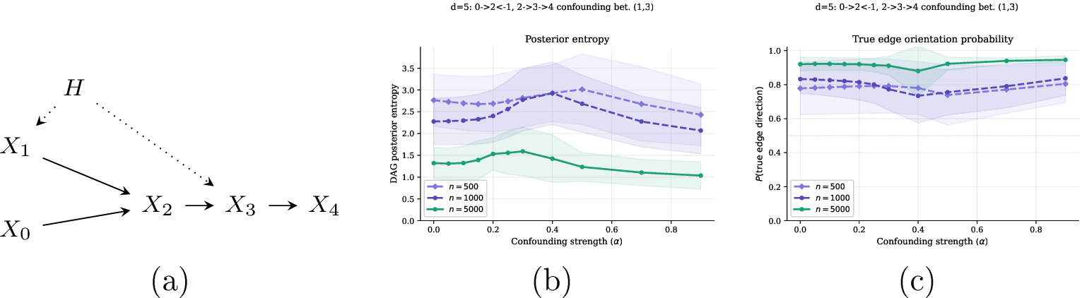
Here, the Posterior entropy (b) rises as competing DAGs gain score, peaks near the critical threshold where structures with and without the spurious edge explain the data equally well, then declines as the posterior concentrates on the new small MEC. True edge probabilities (c) follow a complementary trajectory: they remain stable or briefly decline near the threshold and recover beyond it, consistent with the silent regime. Increasing the sample size \(N\) shifts the transition to lower \(\alpha\), illustrating the sample-size dependence of the critical threshold derived in Section 3.1: more observations make the spurious edge preferred at smaller partial correlation induced by weaker confounding coefficient \(\alpha\).
6 Discussion and Future Research↩︎
In this paper, we derive a critical correlation threshold above which the BGe score favours a spurious edge between latently confounded variables. We show that this threshold shrinks with sample size – meaning that, paradoxically, more observational data makes the posterior more susceptible to confounding, with even weakly induced correlations enough to shift posterior mass toward incorrect causal structures. Beyond the threshold, the impact of confounding is not uniform: it is shaped by how the induced spurious edge interacts with the surrounding collider structure, producing either broad posterior uncertainty (noisy failure) or highly confident but incorrect structures (silent failure). Even in the simple setting considered here, these failure modes reveal striking patterns in posterior behaviour that practitioners would not anticipate from standard reliability cues. The silent regime is particularly concerning, since highly confident posterior edges may still correspond to structurally incorrect causal explanations. In such settings, even partial domain knowledge about potentially confounded variable pairs can be valuable for interpreting posterior confidence more cautiously and motivating additional validation through interventions or sensitivity analysis.
Our analysis is restricted to linear Gaussian SCMs with a single additive Gaussian latent confounder affecting two observed variables. Future work includes extending the characterization to non-Gaussian or discrete settings, multiple interacting confounders, and larger confounded regions involving several variables simultaneously. Another important direction is understanding whether the same structural failure regimes remain observable under practical approximate inference methods on much larger size graphs. More broadly, these results motivate confounder-aware posterior diagnostics and uncertainty measures for Bayesian causal discovery.
7 Derivation of the BGe Confounding Threshold↩︎
We prove Proposition 1. The argument uses three standard facts: decomposability of the BGe score, the large-sample BIC expansion of
Gaussian marginal likelihoods, and the expression of the Gaussian regression likelihood ratio in terms of partial correlation.
Proof of Proposition 1. Let \(P = \operatorname{pa}_G(j)\) denote the current parent set of node \(X_j\), and consider two DAGs \(G\) and \(G'\) that differ only by the candidate edge \(X_k \to X_j\), so that \(\operatorname{pa}_{G'}(j) = P \cup \{k\}\) and all other parent sets coincide.
By decomposability in 4 , \(s(G) = \sum_{i=1}^{n} s(i, \operatorname{pa}_G(i))\). Since \(G\) and \(G'\) agree on every node except \(X_j\), all node-wise terms cancel except that of \(X_j\), giving \[s(G') - s(G) = s(j, P \cup \{k\}) - s(j, P) =: \Delta.\] The edge is favoured by the score precisely when \(\Delta > 0\). For fixed hyperparameters and parent-set size, the BGe marginal likelihood admits the Laplace (BIC) expansion [26], [27] \[s(j, P) = \ell(\hat{\theta}_P) - \frac{m_P}{2}\log N + O_p(1),\] where \(N\) is the number of i.i.d.samples, \(\ell(\hat{\theta}_P)\) is the maximised Gaussian log-likelihood for the regression of \(X_j\) on its parents \(X_P\), and \(m_P\) is the number of local parameters for this regression. Adding \(X_k\) as a parent increases the local dimension by one, \(m_{P \cup \{k\}} - m_P = 1\), so \[\Delta = \ell(\hat{\theta}_{P\cup\{k\}}) - \ell(\hat{\theta}_P) - \frac{1}{2}\log N + O_p(1).\]
For Gaussian linear regression, the maximised log-likelihood difference equals \[\ell(\hat{\theta}_{P\cup\{k\}}) - \ell(\hat{\theta}_P) = \frac{N}{2}\log\!\left(\frac{\mathrm{RSS}_P}{\mathrm{RSS}_{P\cup\{k\}}}\right),\] where \(\mathrm{RSS}_P\) is the residual sum of squares from regressing \(X_j\) on \(X_P\). By the standard partial-correlation identity, \(\mathrm{RSS}_{P \cup \{k\}} / \mathrm{RSS}_P = 1 - \hat{\rho}_{jk \mid P}^2\), where \(\hat{\rho}_{jk \mid P}\) is the sample partial correlation between \(X_j\) and \(X_k\) given \(X_P\). Hence \[\Delta = \frac{N}{2}\log\!\left(\frac{1}{1 - \hat{\rho}_{jk \mid P}^2}\right) - \frac{1}{2}\log N + O_p(1).\]
The first term grows linearly in \(N\) while the penalty grows as \(\log N\), so for large \(N\) the sign of \(\Delta\) is governed by these two terms. The score favours the enlarged parent set (\(\Delta > 0\)) when \[N \log\!\left(\frac{1}{1 - \hat{\rho}_{jk \mid P}^2}\right) > \log N.\]
Under the regular linear Gaussian data-generating process, the sample partial correlation is consistent, \(\hat{\rho}_{jk \mid P} \xrightarrow{p} \rho_{jk \mid P}\) as \(N \to \infty\). The population analogue of the above condition defines a critical partial correlation \(\rho_c\) by \[N \log\!\left(\frac{1}{1 - \rho_c^2}\right) = \log N, \qquad\text{i.e.}\qquad \rho_c^2 = 1 - N^{-1/N}.\] The score favours adding the edge whenever the confounding induces a partial correlation exceeding \(\rho_c\). ◻
-