Autoregressive latent diffusion for 3D molecule generation
July 10, 2026
Abstract
Three-dimensional (3D) molecule generation has been dominated by diffusion models, which achieve strong generation quality but typically require the molecular size to be specified a priori. Recent autoregressive approaches have substantially narrowed the performance gap while naturally supporting variable-length generation and conditioning on partial molecular context. However, balancing unconditional and context-conditioned generation remains challenging. We introduce KRONOS, a latent autoregressive diffusion framework that generates molecules in the latent space of a pre-trained autoencoder, jointly modeling molecular graph topology and geometry, while retaining the flexibility of autoregressive generation. We further introduce a mixed training strategy inspired by Fill-in-the Middle (FIM) paradigm, enabling both unconditional and fragment-conditioned molecular generation within a single left-to-right autoregressive model. Experiments on QM9 and GEOM-Drugs demonstrate that KRONOS achieves leading unconditional generation performance among autoregressive methods, while remaining competitive with diffusion models. Moreover, fragment-conditioned generation is achieved with negligible impact on unconditional generation performance, demonstrating that both generation paradigms can be supported within a single architecture.
1 Introduction↩︎
Generative modeling of three-dimensional (3D) molecules is a central problem in machine learning for drug discovery and molecular design. Recent progress has largely been driven by diffusion [1]–[4] and flow matching [5], which achieve excellent generation quality but typically require the molecular size to be specified a priori.
Autoregressive models provide a complementary paradigm by generating molecules sequentially [6]–[8], naturally supporting variable-length generation and conditioning on partial molecular structures. These capabilities are particularly valuable in medicinal chemistry, where new molecules are often designed by elaborating known scaffolds or functional fragments. Recent autoregressive models [9], [10] have substantially narrowed the performance gap to diffusion-based approaches, making autoregressive generation an increasingly competitive alternative.
At the same time, unified latent representations [4], [11] have emerged as an effective interface for generative modeling by jointly encoding discrete structural information and continuous geometry. Existing latent molecular generators, however, have almost exclusively relied on diffusion-based generation, leaving autoregressive generation largely unexplored.
In this work, we introduce KRONOS, a latent autoregressive diffusion framework for 3D molecule generation. KRONOS performs autoregressive generation directly in the latent space of a pre-trained Unified AutoEncoder (UAE) [3], modeling the joint distribution over latent molecular tokens autoregressively, while parameterizing each conditional distribution with a diffusion objective [12]. Furthermore, an explicit stop-prediction mechanism enables variable-length molecular generation without requiring the molecular size in advance. To support fragment-conditioned generation, we further introduce a mixed training strategy inspired by Fill-in-the-Middle (FIM) paradigm [13] enabling both unconditional and fragment-conditioned molecular generation within a single left-to-right autoregressive model.
Experiments on QM9 and GEOM-Drugs datasets demonstrate that KRONOS achieves leading unconditional performance among autoregressive methods, while remaining competitive with diffusion-based approaches. Furthermore, the results show that enabling fragment-conditioned generation comes at no cost to unconditional generation quality. Our contributions are summarized below:
We introduce KRONOS, a latent autoregressive diffusion framework for 3D molecule generation, combining autoregressive sequence modeling with diffusion-based latent token prediction.
We introduce a fragment-conditioned autoregressive training strategy that enables both unconditional and fragment-conditioned molecule generation within a single autoregressive model.
We show that latent autoregressive generation provides a unified framework for jointly modeling molecular topology and geometry while naturally supporting variable-length generation.
We achieve leading unconditional generation performance among the benchmarked autoregressive methods on QM9 and GEOM-Drugs, while simultaneously enabling accurate fragment-conditioned molecular generation without architectural modifications.
2 Related work↩︎
2.0.0.1 Diffusion-based models for 3D molecule generation
Diffusion models have become the dominant paradigm for 3D molecule generation, achieving state-of-the-art performance across standard benchmarks. Early approaches such as EDM [1] introduced E(3)-equivariant diffusion models that jointly denoise atom coordinates and atom types to generate 3D molecular structures. MiDi [14] extends this framework by jointly generating molecular graph topology and 3D geometry. JODO [2] further develops unified joint 2D/3D diffusion through a dedicated graph transformer that explicitly models interactions between molecular topology and geometry. More recently, ADiT [4] explored latent diffusion over unified all-atom representations, enabling a single transformer-based model to generate both molecules and materials within a shared latent space. Parallel to diffusion, flow-matching approaches such as SemlaFlow [5] learned continuous transport maps from noise to molecular distributions, achieving competitive generation quality while requiring significantly fewer sampling steps.
2.0.0.2 Autoregressive models for 3D molecule generation
Early autoregressive approaches generated molecules sequentially by predicting one atom at a time together with its 3D placement [6], [7]. Symphony [8] subsequently demonstrated that incorporating higher-order E(3)-equivariant representations substantially improves autoregressive molecular generation, narrowing the gap to diffusion-based methods. More recent autoregressive models, including QUETZAL [9] and NEAT [10], combine autoregressive sequence modeling with diffusion-based prediction of continuous molecular geometry. These methods substantially narrow the performance gap to diffusion models while naturally supporting variable-length generation. However, existing autoregressive models still face a performance trade-off between unconditional generation and flexible conditioning on partial molecular structures. Our work addresses this trade-off through a unified autoregressive training framework that jointly supports both objectives.
3 Preliminaries↩︎
3.0.0.1 3D molecule representation
A 3D molecule consists of discrete chemical attributes (atom types and bond connectivity) together with continuous geometry (3D coordinates). This hybrid nature makes joint generative modeling challenging, as it requires simultaneously handling discrete and continuous variables while respecting permutation and SE(3) symmetries. Following previous work [2], [3], we represent a 3D molecule as a tuple \(\mathbf{G} = (\mathbf{H}, \mathbf{A}, \mathbf{X})\), where \(\mathbf{H} \in \mathbb{R}^{|\mathcal{V}| \times d_1}\) encodes atomic features, \(\mathbf{A} \in \mathbb{R}^{|\mathcal{V}| \times |\mathcal{V}| \times d_2}\) is the bond adjacency matrix, and \(\mathbf{X} \in \mathbb{R}^{|\mathcal{V}| \times 3}\) specifies 3D atomic coordinates. \(\mathcal{V}\) represents the set of atoms of \(\mathbf{G}\), while \(d_1\) and \(d_2\) represent the dimension of atomic and bond features, respectively.
3.0.0.2 Unified Autoencoder (UAE).
To obtain a unified representation, we adopt the UAE framework [3], which encodes each atom into a continuous latent vector that jointly captures its chemical identity, bonding environment, and spatial position. The UAE encoder \(\mathcal{E}_{\text{UAE}}\) employs a graph relational transformer [15], which maps a molecule \(\mathbf{G}\) into a latent sequence \(\mathcal{E}_{UAE}(\mathbf{G}) = \mathbf{Z} =\{\mathbf{z}_i \in \mathbb{R}^d \mid i \in \mathcal{V}\}\). A transformer decoder \(\mathcal{D}_{\text{UAE}}\) decodes back the latents into the reconstructed molecule \(\hat{\mathbf{G}} = \mathcal{D}_{\text{UAE}}(\mathbf{Z})\). Notably, both the encoder \(\mathcal{E}_{\text{UAE}}\) and decoder \(\mathcal{D}_{\text{UAE}}\) are permutation equivariant with respect to atom ordering.
3.0.0.3 Autoregressive Diffusion for Continuous Tokens.
To model conditional distributions over continuous tokens, we adopt the Diffusion Loss introduced by [12], which provides a unified framework for continuous-valued generation in both autoregressive (e.g., [16]) and masked modeling settings (e.g., [17], [18]). This formulation replaces discrete token prediction with a denoising objective, enabling flexible modeling of continuous tokens without discretization. In particular, each conditional distribution \(p(\mathbf{x} \mid \mathbf{z})\) is parameterized via a diffusion-based denoising process \[\mathcal{L}(\mathbf{z}, \mathbf{x}) = \mathbb{E}_{t, \varepsilon} \left[ \left\| \varepsilon - \varepsilon_\theta(\mathbf{x}_t \mid t, \mathbf{z}) \right\|^2 \right],\] where \(\mathbf{x}_t\) is a noise-perturbed version of \(\mathbf{x}\) and \(\mathbf{z}\) represents the conditioning context produced by the autoregressive model. This formulation has been successfully applied to 3D molecule generation for modeling continuous 3D geometry [9].
4 Methods↩︎
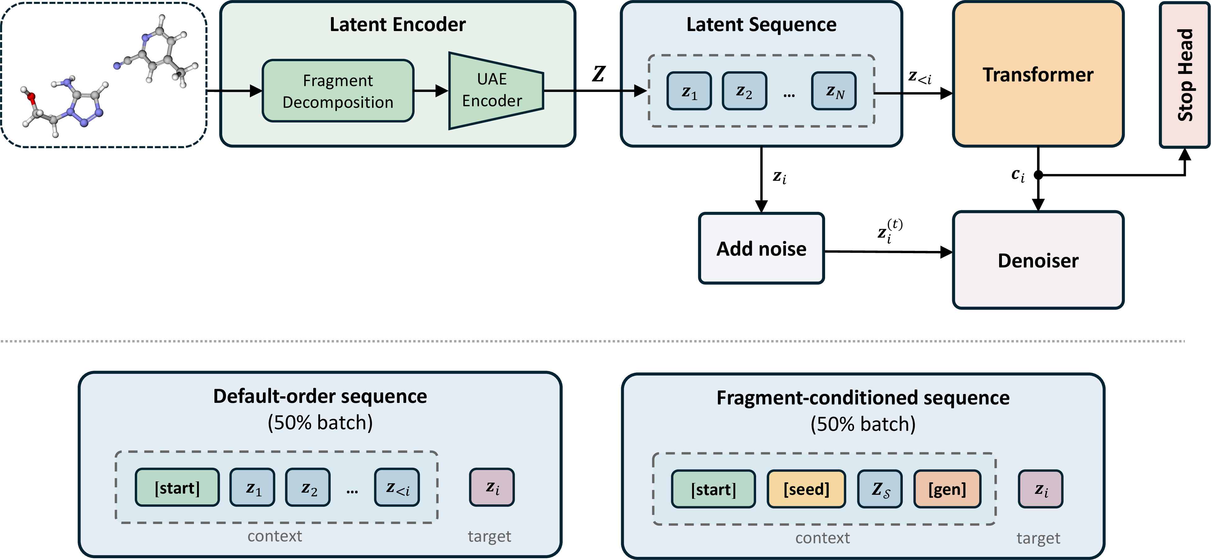
Prior autoregressive approaches to 3D molecule generation operate in data space [9], [19]. This requires the model to learn over heterogeneous discrete and continuous generation targets. We instead perform autoregressive generation directly in the latent space of a pre-trained UAE [3], where each latent token jointly encodes atom identity, bond topology, and 3D geometry. KRONOS combines three key components: (i) autoregressive modeling over latent 3D molecular tokens (Section 4.1), (ii) a mixed autoregressive training strategy supporting both unconditional and fragment-conditioned generation (Section 4.2) and (iii) a Diffusion Loss formulation [12] with a stop classifier for learning sequence termination (Section 4.3). We provide a visual overview of KRONOS in Figure 1.
4.1 Autoregressive Latent Generation↩︎
Our goal is to learn a generative model over latent molecular sequences \(p_\theta(\mathbf{z}_{1:n})\), where each latent token corresponds to an atom. Samples from this distribution are decoded into molecular structures using the UAE decoder \(\mathcal{D}_{\text{UAE}}\). We model the joint distribution over latent tokens \(p_\theta(\mathbf{z}_{1:n})\) using a left-to-right autoregressive factorisation: \[p_\theta(\mathbf{z}_{1:n}) = \prod_{i=1}^{n} p_\theta(\mathbf{z}_i \mid \mathbf{z}_{<i}), \label{eq:lr95ar}\tag{1}\] where generation is initialized with a special \([\mathrm{START}]\) token. At each step \(i\), a causal transformer encodes the preceding tokens into a context representation \[\mathbf{c}_i = \mathrm{Transformer}([\mathrm{START}], \mathbf{z}_1, \ldots, \mathbf{z}_{i-1}), \label{eq:transf95context}\tag{2}\] which conditions a diffusion model used to parameterize \(p_\theta(\mathbf{z}_i \mid \mathbf{z}_{<i})\) (described in Section 4.3.0.1). As the latent space does not admit a natural end-of-sequence token, we model sequence termination separately via a stop classifier \(p_\theta([\mathrm{STOP}] \mid \mathbf{c}_i)\) (described in Section 4.3.0.2). During training, the autoregressive factorization in Eq. 1 corresponds to the default-order sequence, which follows the token ordering inherited from the input molecules, and is used for unconditional (de novo) molecule generation.
4.2 Fragment-conditioned generation↩︎
Previous autoregressive models for 3D molecule generation employ a fixed atom ordering [9]. While effective for unconditional generation, such atom-level orderings do not support conditioning generation on arbitrary molecular fragments. To address this, we introduce a mixed autoregressive training strategy inspired by Fill-in-the-Middle (FIM) paradigm [13], originally proposed to unlock document-infilling capabilities within left-to-right transformer models and later extended to protein language models [20]. To support fragment-conditioned generation, we additionally re-train the UAE encoder to produce fragment-local latent representations, as described in Appendix 8.2. During training, each molecule is transformed into either a default-order sequence (Section 4.1) or a fragment-conditioned sequence with probabilities \(1-p_{f}\) and \(p_{f}\), respectively, where \(p_f\) denotes the fragment-conditioning probability. We use \(p_f = 0.5\) throughout the main experiments and study the effect of varying \(p_f\) in Appendix 8.7. The fragment-conditioned sequence construction can be viewed as defining autoregressive factorisations at the fragment level rather than at the atom level. We introduce this perspective below.
4.2.0.1 Permutation space
Because the UAE encoder–decoder pair \((\mathcal{E}_{\mathrm{UAE}},\mathcal{D}_{\mathrm{UAE}})\) is permutation equivariant, every permutation \(\pi\in S_n\) induces a valid autoregressive factorisation of the joint latent distribution: \[p_\theta(\mathbf{z}_{1:n}) = \prod_{i=1}^{n} p_\theta\!\left(\mathbf{z}_{\pi(i)} \mid \mathbf{z}_{\pi(<i)} \right).\] Order-agnostic autoregressive (OA-AR) models [21], [22] treat \(\pi\) as a latent variable and maximise the expected log-likelihood over \(S_n\). Because the full expectation is intractable, they optimise the variational lower bound \[\label{eq:oaar95obj} \log p_\theta(\mathbf{z}) \;\ge\; \mathbb{E}_{\pi\sim S_n}\!\left[\, \sum_{i=1}^{n}\log p_\theta\!\left( \mathbf{z}_{\pi(i)} \mid \mathbf{z}_{\pi(<i)}\right) \right],\tag{3}\] which can be estimated with Monte-Carlo sampling of permutations and positions, as originally proposed by [21] and later reformulated to enable efficient, single-step training [23]. Rather than marginalizing over \(S_n\) as in OA-AR, we instead define autoregressive factorisations based on molecular fragments. Specifically, each molecule is decomposed into chemically meaningful fragments. A random subset of these fragments is then selected as the conditioning context, and a single deterministic ordering is assigned to the resulting conditioning and generation sequences.
4.2.0.2 Fragment decomposition
To construct fragment-conditioned training sequences, each molecule is partitioned into \(K\) fragments \(\{\mathcal{F}_0,\ldots,\mathcal{F}_{K-1}\}\) using a BRICS-based decomposition [24], a common fragmentation strategy employed in molecular machine learning [25]–[27]. Hydrogens bonded to heteroatoms are retained within their parent fragment, while carbon-bound structural hydrogens are assigned to a dedicated pseudo-fragment \(\mathcal{F}_H\). This yields a collection of contiguous fragment blocks used to construct fragment-based orderings. Full details are provided in Appendix 8.1.
4.2.0.3 Fragment-conditioned sequence
Given the fragment decomposition above, we sample a seed size \(s \sim \mathrm{Uniform}\{1,\ldots,K-1\}\) and sample a fragment subset \(\mathcal{S} \subset \{\mathcal{F}_0,\ldots,\mathcal{F}_{K-1}\}\) uniformly among all subsets of size \(s\). The selected subset \(\mathcal{S}\) serves as the seed, while the complement \(\mathcal{S}^c\) defines the generation target. For a sampled subset \(\mathcal{S}\), we construct \(\mathbf{Z}_{\mathcal{S}}\) and \(\mathbf{Z}_{\mathcal{S}^c}\) as the latent token sequences associated with fragments in \(\mathcal{S}\) and its complement \(\mathcal{S}^c\), respectively. Within each sequence, fragments are ordered deterministically according to their assigned fragment indices, while atoms within each fragment follow a deterministic depth-first search (DFS) traversal (see Appendix 8.1 for details). For each sampled fragment partition, this procedure defines a unique autoregressive sequence. The latent tokens associated with structural hydrogens \(\mathbf{Z}_{\mathcal{F}_H}\) are excluded from the fragment sampling procedure. Instead, they are deterministically placed after \(\mathbf{Z}_{\mathcal{S}^c}\) in every training sequence and generated autoregressively. The resulting training sequence is
\[[\mathrm{START}]\; [\mathrm{SEED}]\; \mathbf{Z}_{\mathcal{S}}\; [\mathrm{GEN}]\; \mathbf{Z}_{\mathcal{S}^c}\; \mathbf{Z}_{\mathcal{F}_H}\; [\mathrm{STOP}],\]
where sentinel tokens mark the conditioning and generation regions. Conditioned on the seed sequence \(\mathbf{Z}_{\mathcal{S}}\), the remaining tokens are generated autoregressively: \[p_\theta(\tilde{\mathbf{Z}}_{\mathcal{S}^c} \mid \mathbf{Z}_{\mathcal{S}}) = \prod_{j=1}^{m} p_\theta(\mathbf{z}_{r_j}\mid \mathbf{Z}_{\mathcal{S}}, \mathbf{z}_{r_{<j}}),\] where \(\tilde{\mathbf{Z}}_{\mathcal{S}^c} = (\mathbf{Z}_{\mathcal{S}^c},\mathbf{Z}_{\mathcal{F}_H} )\). Unlike order-agnostic autoregressive training [21], which requires marginalizing over multiple token orderings, our formulation assigns a single deterministic factorization to each sampled fragment partition by fixing both the ordering of fragments and the ordering of atoms within each fragment. Diversity arises from the choice of conditioning and generation fragments rather than from multiple orderings of the same partition. During training, we sample the seed cardinality uniformly and then sample uniformly among fragment subsets of that cardinality. This exposes the model to conditioning contexts of varying sizes.
4.3 Training objective↩︎
4.3.0.1 Diffusion loss
To model autoregressive conditionals \(p_\theta(\mathbf{z}_i \mid \mathbf{z}_{<i})\), we adopt a Diffusion Loss formulation [12] and model each using a diffusion process in the continuous latent space. Let \(\mathbf{c}_i\) denote the causal transformer context at step \(i\). To model the distribution of the next latent token \(\mathbf{z}_i\), we adopt a Variance-Preserving (VP) forward process [28] that perturbs \(\mathbf{z}_i\) with Gaussian noise: \[\mathbf{z}_i^{(t)} = \alpha_t \mathbf{z}_i + \sigma_t \varepsilon, \quad t \sim \mathcal{U}[0,1],\; \varepsilon \sim \mathcal{N}(0,I) \, ,\] where \(\alpha_t\) and \(\sigma_t\) denote the signal and noise coefficients of the VP noise schedule. The denoising network \(\varepsilon_\theta(\cdot)\) is implemented as a residual Multi-Layer Perceptron (MLP) with Adaptive Layer Normalization (AdaLN) conditioning [12]. The network predicts the injected noise \(\varepsilon\) conditioned on the noisy latent, the autoregressive context, and the diffusion timestep. Following standard diffusion training [29], we optimize the noise prediction objective \[\label{eq:diff95loss} \mathcal{L}_{\mathrm{diff}} = \mathbb{E}_{(\mathbf{z}_i,\mathbf{c}_i),\,t,\,\varepsilon} \left[ \left\| \varepsilon_\theta(\mathbf{z}_i^{(t)}, \mathbf{c}_i, t) - \varepsilon \right\|^2 \right] \;,\tag{4}\] where \(\mathbf{c}_i\) denotes the autoregressive transformer context (Eq. 2 ), and \(\mathbf{z}_i\) and \(\mathbf{z}_i^{(t)}\) denote the clean and noisy latent targets, respectively.
4.3.0.2 Stop loss
Unlike autoregressive models operating directly in data space [9], [10], our latent-space formulation does not contain a dedicated end-of-sequence token. Consequently, sequence termination cannot be modeled through standard next-token prediction. To address this, we train a lightweight stop classifier \(\text{MLP}_{\text{stop}}\) operating on the transformer hidden states \(\mathbf{c}_i\). At each autoregressive step, the classifier predicts the probability that generation should terminate conditioned on the current context: \[p_\theta([\mathrm{STOP}] \mid \mathbf{c}_i)= \sigma\!\left( \mathrm{MLP}_{\mathrm{stop}}(\mathbf{c}_i)\right),\] where \(\sigma(\cdot)\) denotes the sigmoid function. The classifier is trained jointly with the diffusion model using a binary cross-entropy objective \[\label{eq:stop95loss} \mathcal{L}_{\mathrm{stop}} = \mathbb{E}_{(\mathbf{c}_i, y_i^{\mathrm{stop}})} \left[ \mathrm{BCE}\!\left( p_\theta([\mathrm{STOP}] \mid \mathbf{c}_i), y_i^{\mathrm{stop}} \right) \right].\tag{5}\] where \(y_i^{\mathrm{stop}} \in \{0,1\}\) is one when \(\mathbf{c}_i\) corresponds to the context after the final latent token, and zero otherwise. This auxiliary objective enables the model to infer molecular size dynamically during generation, without requiring a predefined number of atoms.
4.3.0.3 Global objective
All components, the transformer, the MLP denoiser, and the stop classifier, are trained jointly, while the pre-trained UAE encoder is kept frozen. The full objective is: \[\mathcal{L} = \mathcal{L}_{\mathrm{diff}} + \lambda_{\mathrm{stop}}\mathcal{L}_{\mathrm{stop}} \;,\] where \(\mathcal{L}_{\mathrm{diff}}\), \(\mathcal{L}_{\text{stop}}\) are defined in Eq. 4 , Eq. 5 , respectively, and \(\lambda_{\mathrm{stop}}\) is empirically set to \(1.0\).
5 Experiments↩︎
We evaluate KRONOS on three complementary tasks. First, we assess unconditional 3D molecule generation on the QM9 and GEOM-Drugs benchmarks (Tables [table:metrics95qm9953d] and 2), comparing against both autoregressive and diffusion-based baselines. Second, we evaluate fragment-conditioned molecular generation (Table 3), measuring the model’s ability to generate coherent molecular structures from partial molecular context, inspired by the setting introduced by [10]. Third, motivated by known limitations of standard evaluation metrics for 3D molecule generation [5], [10], we further assess the physical plausibility of generated conformations through semi-empirical geometry optimization using GFN2-xTB [30]. Additional experiments focusing on 2D molecule generation are provided in Appendix 8.5.
5.1 Experimental setup↩︎
5.1.0.1 Datasets
We evaluate our framework on the QM9 [31] and GEOM-Drugs [32] datasets, following standard benchmarks for 3D molecule generation. For QM9, we use the same train/validation/test split established in existing work [2], [3], resulting in \(97,609\)/\(14,405\)/\(12,405\) molecules. Similarly, for GEOM-Drugs we follow the pre-processing and train/validation/test splits utilized in existing literature [14], retaining the five lowest-energy conformers per molecule. This results in \(1,172,532\)/\(146,405\)/\(146,793\) conformers for training, validation, and testing, respectively.
5.1.0.2 Baselines
We compare the proposed method with several existing autoregressive and diffusion baselines for 3D molecule generation. Autoregressive baselines include G-SchNet [6], G-SphereNet [7], Symphony [8], QUETZAL [9], NEAT [10]. Diffusion models include EDM [1], MiDi [14], ADiT [4] and JODO [2]. We additionally include SemlaFlow [5] as a flow matching baseline. We do not report performance of UDM-3D [3], because we are unable to reproduce reasonable results utilizing the source code, and pre-trained checkpoints or pre-generated molecules are unavailable at the time of writing.
5.1.0.3 Metrics
We evaluate generated molecules using standard metrics for 3D molecule generation, assessing both chemical correctness and geometric fidelity. Specifically, we report validity and stability of reconstructed molecular graphs together with Maximum Mean Discrepancy (MMD) [33] between generated and reference bond length, bond angle, and dihedral angle distributions. Complete metric definitions are provided in Appendix 8.4.
| Model | 3D Validity (\(\uparrow\)) | 3D AtomStable (\(\uparrow\)) | 3D MolStable (\(\uparrow\)) | Bond length (\(\downarrow\)) | Bond angle (\(\downarrow\)) | Dihedral angle (\(\downarrow\)) |
| (%) | (%) | (%) | \((\times 10^{-2})\) | \((\times 10^{-2})\) | \((\times 10^{-3})\) | |
| QM9 | \(98.4\phantom{_{\pm 0.0}}\) | \(99.53\phantom{_{\pm 0.00}}\) | \(96.3\phantom{_{\pm 0.0}}\) | \(0.003\phantom{_{\pm}}\) | \(1.06\phantom{_{\pm 0.00}}\) | \(0.05\phantom{_{\pm 0.00}}\) |
| Diffusion / Flow | ||||||
| ADiT* | \(79.3\phantom{_{\pm 0.0}}\) | \(76.43\phantom{_{\pm 0.00}}\) | \(7.6\phantom{_{\pm 0.0}}\) | \(111.5\phantom{_{\pm 0.0}}\) | \(14.90\phantom{_{\pm 0.00}}\) | \(3.60\phantom{_{\pm 0.00}}\) |
| JODO* | \(96.3\phantom{_{\pm 0.0}}\) | \(\mathbf{99.25}\phantom{_{\pm 0.00}}\) | \(\mathbf{93.6}\phantom{_{\pm 0.0}}\) | \(38.1\phantom{_{\pm 0.0}}\) | \(2.23\phantom{_{\pm 0.00}}\) | \(1.37\phantom{_{\pm 0.00}}\) |
| EDM† | \(95.3_{\pm0.1}\) | \(97.56_{\pm0.19}\) | \(87.6_{\pm0.1}\) | \(23.7_{\pm2.3}\) | \(2.21_{\pm0.06}\) | \(\underline{0.50}_{\pm0.10}\) |
| SemlaFlow** | \(85.8_{\pm0.1}\) | \(97.07_{\pm0.03}\) | \(78.6_{\pm0.2}\) | \(75.2_{\pm0.8}\) | \(1.94_{\pm0.02}\) | \(1.55_{\pm0.21}\) |
| MiDi** | \(95.3_{\pm 0.3}\) | \(98.21_{\pm 0.05}\) | \(83.5_{\pm 0.2}\) | \(110.5_{\pm 1.7}\) | \(3.00_{\pm 0.10}\) | \(0.80_{\pm 0.10}\) |
| Autoregressive | ||||||
| Symphony* | \(68.1\phantom{_{\pm 0.0}}\) | \(90.75\phantom{_{\pm 0.00}}\) | \(43.9\phantom{_{\pm 0.0}}\) | \(19.4\phantom{_{\pm 0.0}}\) | \(11.00\phantom{_{\pm 0.00}}\) | \(2.06\phantom{_{\pm 0.00}}\) |
| G-SchNet* | \(80.1\phantom{_{\pm 0.0}}\) | \(93.71\phantom{_{\pm 0.00}}\) | \(63.7\phantom{_{\pm 0.0}}\) | \(41.5\phantom{_{\pm 0.0}}\) | \(9.25\phantom{_{\pm 0.00}}\) | \(6.49\phantom{_{\pm 0.00}}\) |
| G-SphereNet* | \(16.4\phantom{_{\pm 0.0}}\) | \(67.82\phantom{_{\pm 0.00}}\) | \(14.0\phantom{_{\pm 0.0}}\) | \(27.8\phantom{_{\pm 0.0}}\) | \(37.60\phantom{_{\pm 0.00}}\) | \(14.30\phantom{_{\pm 0.00}}\) |
| QUETZAL** | \(94.8_{\pm 0.1}\) | \(98.28_{\pm 0.04}\) | \(87.4_{\pm 0.2}\) | \(40.1_{\pm 1.1}\) | \(2.20_{\pm 0.10}\) | \(\mathbf{0.41}_{\pm 0.03}\) |
| NEAT** | \(93.4_{\pm 0.1}\) | \(98.09_{\pm 0.02}\) | \(84.0_{\pm 0.3}\) | \(33.1_{\pm 0.1}\) | \(1.90_{\pm 0.10}\) | \(4.30_{\pm 0.20}\) |
| KRONOS (ours) | \(\mathbf{97.3}_{\pm 0.1}\) | \(\underline{99.07}_{\pm 0.02}\) | \(\underline{92.6}_{\pm 0.1}\) | \(\mathbf{4.8}_{\pm 0.6}\) | \(\mathbf{1.33}_{\pm 0.03}\) | \(1.00_{\pm 0.10}\) |
| Model | 3D Validity (\(\uparrow\)) | 3D AtomStable (\(\uparrow\)) | 3D MolStable (\(\uparrow\)) | Bond length (\(\downarrow\)) | Bond angle (\(\downarrow\)) | Dihedral angle (\(\downarrow\)) | |
| (%) | (%) | (%) | |||||
| GEOM | \(96.6\phantom{_{\pm 0.0}}\) | \(86.17\phantom{_{\pm 0.00}}\) | \(2.80\phantom{_{\pm 0.00}}\) | \(0.253\phantom{_{\pm 0.000}}\) | \(0.2695\phantom{_{\pm 0.0000}}\) | \(0.0153\phantom{_{\pm 0.0000}}\) | |
| Diffusion / Flow | |||||||
| ADiT* | \(\underline{97.3}\phantom{_{\pm 0.0}}\) | \(75.46\phantom{_{\pm 0.00}}\) | \(0.12\phantom{_{\pm 0.00}}\) | \(1.323\phantom{_{\pm 0.000}}\) | \(1.0474\phantom{_{\pm 0.0000}}\) | \(0.0548\phantom{_{\pm 0.0000}}\) | |
| JODO* | \(95.6\phantom{_{\pm 0.0}}\) | \(84.49\phantom{_{\pm 0.00}}\) | \(1.11\phantom{_{\pm 0.00}}\) | \(\underline{0.089}\phantom{_{\pm 0.000}}\) | \(\mathbf{0.0099\phantom{_{\pm 0.0000}}}\) | \(\mathbf{0.0005\phantom{_{\pm 0.0000}}}\) | |
| EDM† | \(90.5_{\pm 0.6}\) | \(83.35_{\pm 0.05}\) | \(1.01_{\pm0.04}\) | \(0.865_{\pm0.005}\) | \(0.8368_{\pm0.0060}\) | \(0.0567_{\pm0.0004}\) | |
| SemlaFlow** | \(92.4_{\pm 0.2}\) | \(84.10_{\pm 0.09}\) | \(2.17_{\pm0.24}\) | \(0.569_{\pm0.001}\) | \(0.1241_{\pm0.0015}\) | \(\underline{0.0007}_{\pm0.0000}\) | |
| MiDi** | \(92.0_{\pm0.4}\) | \(75.48_{\pm0.16}\) | \(0.30_{\pm0.04}\) | \(0.113_{\pm0.001}\) | \(\underline{0.0915}_{\pm0.0029}\) | \(0.0046_{\pm0.0003}\) | |
| Autoregressive | |||||||
| QUETZAL† | \(93.8_{\pm 0.2}\) | \(\underline{86.27}_{\pm 0.03}\) | \(\underline{2.04}_{\pm 0.06}\) | \(0.882_{\pm 0.008}\) | \(0.9370_{\pm 0.0068}\) | \(0.0614_{\pm 0.0015}\) | |
| NEAT** | \(\mathbf{98.1}_{\pm 0.1}\) | \(81.16_{\pm 0.04}\) | \(0.50_{\pm 0.01}\) | \(1.194_{\pm 0.002}\) | \(1.3939_{\pm 0.0342}\) | \(0.1543_{\pm 0.0012}\) | |
| KRONOS (ours) | \(94.7_{\pm0.2}\) | \(\mathbf{86.45}_{\pm0.03}\) | \(\mathbf{2.70}_{\pm0.10}\) | \(\mathbf{0.048}_{\pm0.003}\) | \(0.0944_{\pm0.0004}\) | \(\mathbf{0.0005}\pm_{0.0002}\) | |
5.2 Results↩︎
5.2.0.1 Unconditional molecular generation
Results for unconditional generation on QM9 and GEOM-Drugs are reported in Tables [table:metrics95qm9953d] and 2, respectively. On QM9, KRONOS achieves the highest validity (\(\mathbf{97.3}\%\)) and the strongest overall performance among autoregressive methods. Despite being trained jointly for unconditional and fragment-conditioned generation, KRONOS remains competitive with leading diffusion models (e.g. JODO) across all reported metrics. As shown in Appendix 8.7, reducing the fragment-conditioning probability \(p_f\) further improves unconditional generation performance, suggesting that the remaining gap is primarily due to the joint training objective rather than the autoregressive latent space formulation. Compared with recent autoregressive baselines such as QUETZAL and NEAT, these results demonstrate that latent autoregressive generation can substantially improve both chemical validity and geometric fidelity. On the more challenging GEOM-Drugs benchmark, KRONOS achieves the strongest overall performance among the evaluated baselines.
5.2.0.2 Assessment of generated conformers stability
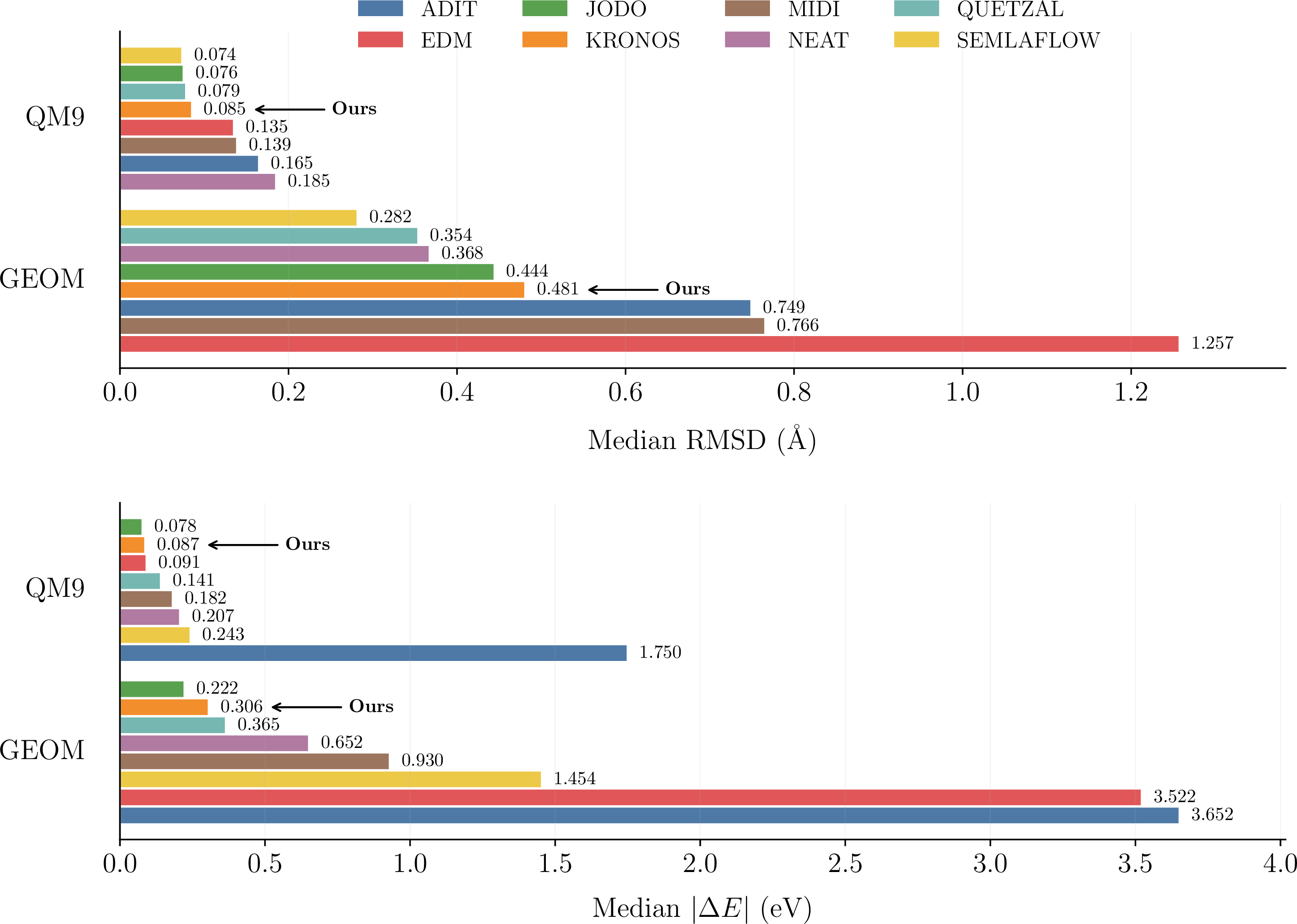
While the molecular stability criterion (3D MolStable) introduced by [1] has become a standard evaluation metric for molecule generation, it relies on heuristic bond-assignment procedures that can be sensitive to aromatic systems and distance thresholds [5], [8], [10]. Consequently, it primarily evaluates whether a generated atomic point cloud admits a chemically plausible molecular graph, rather than directly assessing the physical plausibility of the generated conformation. To complement this graph-based evaluation, we perform semi-empirical quantum-chemical refinement using GFN2-xTB [30]. For each generated molecule, we compute its single-point energy before geometry optimization with xTB and report (i) the Root Mean Square Distance (RMSD) between the generated and optimized conformations after optimal rigid-body alignment using the Kabsch algorithm [34], and (ii) the absolute energy difference \(|\Delta E|\) between the corresponding structures. Lower RMSD indicates that the generated conformation is geometrically closer to the xTB-optimized structure, while lower \(|\Delta E|\) indicates that it is energetically closer to the xTB-optimized structure. Figure 2 summarizes the results. On QM9, KRONOS achieves competitive median RMSD and median energy difference, indicating that the generated conformations require only limited relaxation during quantum-chemical optimization. On the more challenging GEOM benchmark, JODO achieves the strongest overall performance, while KRONOS consistently outperforms several existing diffusion-based and autoregressive baselines on both geometric and energetic criteria. Overall, these results demonstrate that the proposed autoregressive latent generation strategy produces geometrically accurate and energetically plausible molecular conformations.
5.2.0.3 Fragment-conditioned molecule generation
We evaluate whether the proposed framework can generate chemically coherent 3D molecules from partial molecular context. This task follows the spirit of prefix completion introduced by [10]. However, rather than conditioning on a fixed set of manually designed scaffolds, we construct conditioning prefixes by our fragment decomposition scheme (Appendix 8.1) applied to molecules from the GEOM-Drugs test set, and treat each resulting fragment as an independent conditioning context. The same fragment-derived prefixes are used to evaluate other autoregressive models (KRONOS, NEAT, and QUETZAL).
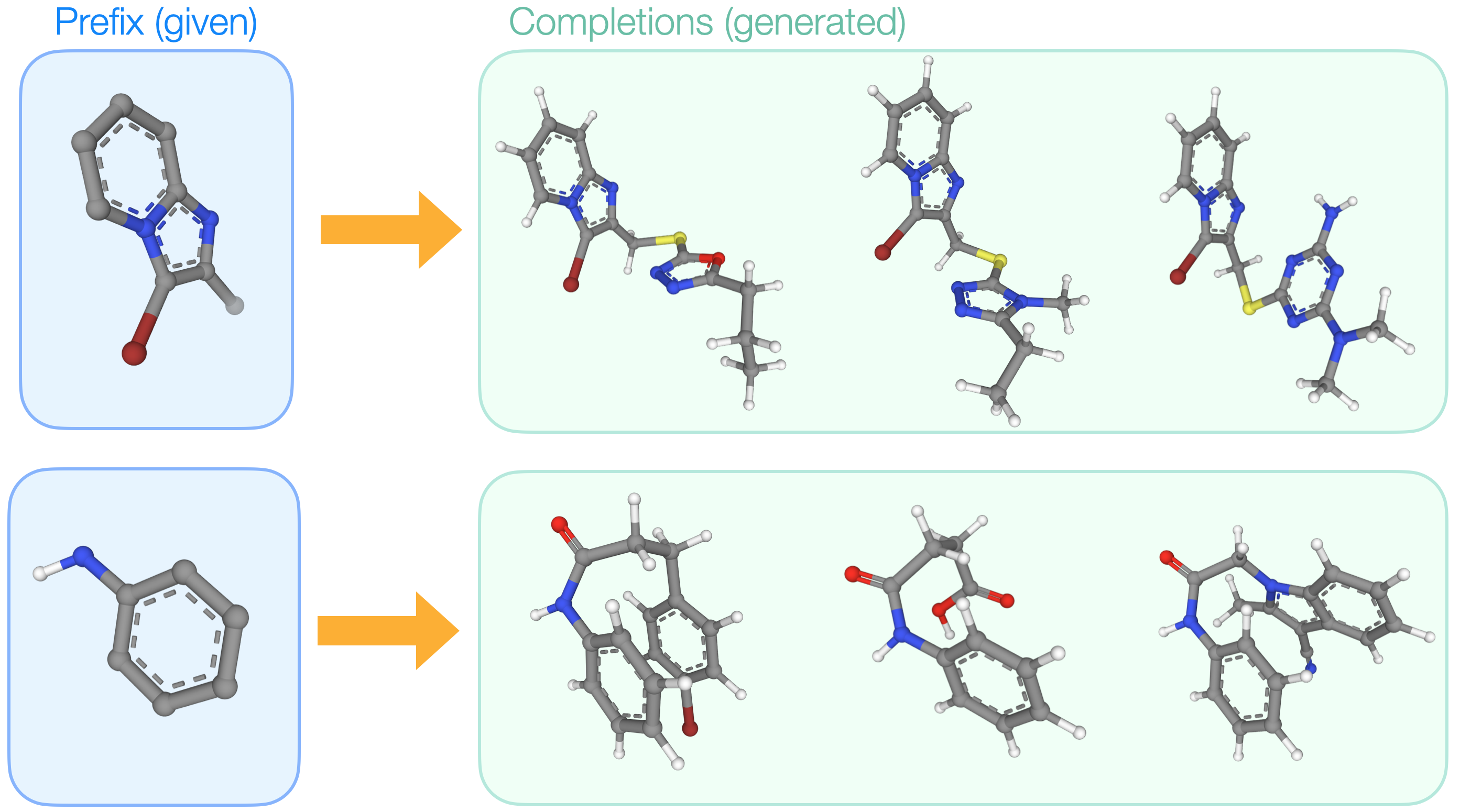
In total, we collect \(\sim\) \(15\)k molecule-fragment pairs. For each pair, we sample \(3\) completions and report Best@3 and Mean@3 in Table 3. Mean@3 computes the average value of each evaluation metric across the three completions, whereas Best@3 reports the best value achieved among the three completions for each metric.
| Mean@3 | Best@3 | |||||
|---|---|---|---|---|---|---|
| 2-4 (lr)5-7 Model | 3D Validity | 3D AtomStable | 3D MolStable | 3D Validity | 3D AtomStable | 3D MolStable |
| QUETZAL† | \(48.7_{\pm0.6}\) | \(67.6_{\pm0.2}\) | \(0.2_{\pm0.1}\) | \(70.6_{\pm0.7}\) | \(74.2_{\pm0.2}\) | \(0.5_{\pm0.1}\) |
| NEAT* | \(\mathbf{93.7}_{\pm0.3}\) | \(\mathbf{83.4}_{\pm0.1}\) | \(\underline{0.8}_{\pm0.1}\) | \(\mathbf{97.4}_{\pm0.2}\) | \(\mathbf{87.9}_{\pm0.1}\) | \(\mathbf{2.1}_{\pm0.2}\) |
| KRONOS (ours) | \(\underline{79.7}_{\pm0.4}\) | \(\underline{82.1}_{\pm0.1}\) | \(\mathbf{0.9}_{\pm0.1}\) | \(\underline{96.2}_{\pm0.3}\) | \(\underline{86.5}_{\pm0.1}\) | \(\underline{1.8}_{\pm 0.2}\) |
11pt
Overall, the results demonstrate that fragment-conditioned generation can be effectively learned without a fully permutation-invariant model. Compared to QUETZAL, which follows a similar autoregressive formulation, KRONOS substantially improves fragment-conditioned generation across all evaluation metrics. This suggests that exposing the model during training to diverse fragment-conditioning distributions through a FIM-style data transformation is sufficient to endow a standard autoregressive model with robust molecular completion capabilities, while preserving excellent unconditional generation performance. Indeed, KRONOS remains highly competitive for unconditional molecule generation on both QM9 and GEOM-Drugs.
6 Limitations and future work↩︎
KRONOS inherits several limitations from the underlying latent autoregressive formulation. First, the model relies on a pre-trained autoencoder [3] to define the latent molecular representation. Consequently, generation quality is ultimately bounded by the expressiveness and reconstruction fidelity from the underlying latent space. Improvements in latent representation learning may therefore translate directly into improved generative performance. Second, while fragment-conditioned training substantially improves completion from partial molecular context, KRONOS does not possess the full permutation invariance of specialized architectures such as NEAT [10]. Third, our fragment decomposition relies on a fixed BRICS-derived partitioning scheme. While this provides chemically meaningful conditioning units, alternative decomposition strategies may expose different structural regularities and lead to improved performance. Learning fragment abstractions jointly with the generative model remains an interesting direction for future work. Finally, while we focus on unconditional and fragment-conditioned molecular generation, the proposed framework could be naturally extended to property-guided molecular design. In particular, future work could condition generation on a molecular fragment while simultaneously optimizing for desired molecular properties.
7 Conclusion↩︎
We introduced KRONOS, a latent autoregressive diffusion framework for 3D molecule generation. By operating in the unified latent space of a pre-trained autoencoder, KRONOS leverages a unified representation of molecular graph topology and geometry, providing an effective foundation for autoregressive 3D molecule generation. Conceptually, this design combines the strengths of autoregressive and diffusion models. Like autoregressive models, KRONOS generates one atom at a time, naturally supporting variable-length generation and conditioning on partial structures, in contrast to most existing diffusion and flow-based approaches, which require the molecular size to be specified before generation. Unlike prior autoregressive models, which operate in data space and jointly predict discrete atom and bond types alongside continuous coordinates, KRONOS replaces the mixed discrete–continuous target with a single continuous token per atom. Beyond unconditional generation, we introduced a fragment-conditioned training strategy inspired by the Fill-in-the-Middle paradigm, enabling fragment-conditioned molecule generation without architectural modifications. Experiments on QM9 and GEOM-Drugs demonstrate leading performance among autoregressive methods while matching or surpassing diffusion-based approaches. Furthermore, semi-empirical geometry optimization suggests that generated conformations lie close to physically plausible regions of conformational space. Overall, our results indicate that latent autoregressive generation provides a promising alternative to existing data-space autoregressive and diffusion-based approaches, while naturally supporting flexible generation strategies for molecular design and discovery.
Code availability statement↩︎
The source code and model checkpoints required to reproduce the experiments presented in this work will be made publicly available upon publication.
Acknowledgments↩︎
F.O., K.E.J., A.M.G., Y.Li acknowledge the AI for Chemistry: AIchemy hub for funding (EPSRC grant EP/Y028775/1 and EP/Y028759/1). G.R. acknowledges Imperial College London for funding through President’s PhD Scholarships. The authors acknowledge the use of resources provided by the Isambard-AI National AI Research Resource (AIRR). Isambard-AI is operated by the University of Bristol and is funded by the UK Government’s Department for Science, Innovation and Technology (DSIT) via UK Research and Innovation; and the Science and Technology Facilities Council [ST/AIRR/I-A-I/1023].
8 Appendix↩︎
8.1 Fragment-based molecular decomposition↩︎
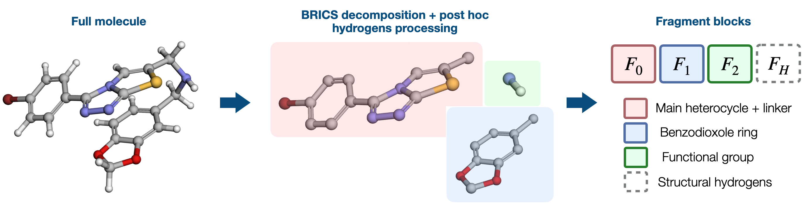
Rather than considering arbitrary atom permutations, we decompose each molecule into chemically meaningful fragments and assign a deterministic ordering within each fragment. During training, random fragment partitions define the conditioning and generation regions, yielding diverse fragment-conditioned autoregressive generation tasks while avoiding arbitrary atom-level permutations. Fragment boundaries are obtained from a BRICS-based decomposition [24], which cleaves bonds at retrosynthetically meaningful sites to produce chemically coherent building blocks, and has been explored in molecular generative modeling [27], [35]. We further refine this decomposition by retaining heteroatom-bound hydrogens, such as hydroxyl or amine hydrogens, within their parent fragment, while carbon-bound structural hydrogens are assigned to a separate pseudo-fragment. This preserves pharmacophoric functional groups as coherent units. Let \(\mathcal{V}^H\) denote the heavy-atom set of a molecule. The BRICS-based decomposition induces a partition \(\mathcal{V}^H=\mathcal{F}_0 \sqcup \cdots \sqcup \mathcal{F}_{K-1}\). Hydrogens are then incorporated according to chemical role. Hydrogens bonded to heteroatoms are assigned to the same fragment as their parent atom, preserving functional groups such as \(\mathrm{-OH}\), \(\mathrm{-NH_2}\), and \(\mathrm{-SH}\) as single units. In contrast, hydrogens bonded to carbon are collected into a separate pseudo-fragment \(\mathcal{F}_H\), which is always appended after all fragment blocks. Carbon-bound hydrogens are largely determined by the heavy-atom scaffold and contribute little independent structural information. Within each fragment \(\mathcal{F}_k\), atoms are ordered using a deterministic depth-first search (DFS) traversal of the fragment subgraph, yielding a fixed ordering for each fragment. During training, the fragment set is randomly partitioned into conditioning and generation fragments while preserving the fixed DFS ordering within each fragment and the fragment ordering induced by the BRICS decomposition. Structural hydrogens are always appended last. Consequently, the model is exposed to many fragment-conditioned generation tasks while avoiding arbitrary atom-level permutations. We provide an illustrative example of the adopted decomposition in Figure 4.
8.2 Fragment-local latent encoding↩︎

In the original UAE architecture [3], latent representations are computed through message passing across the full molecular graph, allowing each latent token to aggregate information from progressively larger molecular neighborhoods. Consequently, the latent representation of each fragment depends not only on its internal structure but also on atoms belonging to neighboring fragments. However, our fragment-conditioned generation setting requires latent representations that can be computed for fragments in isolation at inference time. To achieve this, we modify the encoder connectivity during UAE training. Given a fragment decomposition \(\{\mathcal{F}_0,\dots,\mathcal{F}_{K-1}\}\) of a molecular graph \(\mathbf{G}\), we remove all inter-fragment edges prior to encoder message passing, restricting information propagation to atoms within the same fragment. Importantly, this modification affects only the graph used by the encoder to compute latent representations. The decoder continues to reconstruct the complete molecule graph, including inter-fragment connectivity and global 3D geometry. Consequently, latent tokens are encouraged to capture fragment-local information, while the decoder remains responsible for integrating information across fragments and recovering global structures. Empirically, we observe that UAE reconstruction performance remains unchanged even under the extreme setting in which all inter-atomic edges are removed during encoding, causing each atom to be encoded independently. This suggests that accurate reconstruction does not require latent representations to explicitly encode global molecular context. We hypothesize that this behavior stems from the decoder jointly attending over all latent tokens during decoding, while the initial atom embeddings already encode atom identity and spatial information. Consequently, global structural relationships can be recovered during decoding, providing substantial flexibility in the encoder connectivity.
8.3 Fragment statistics↩︎
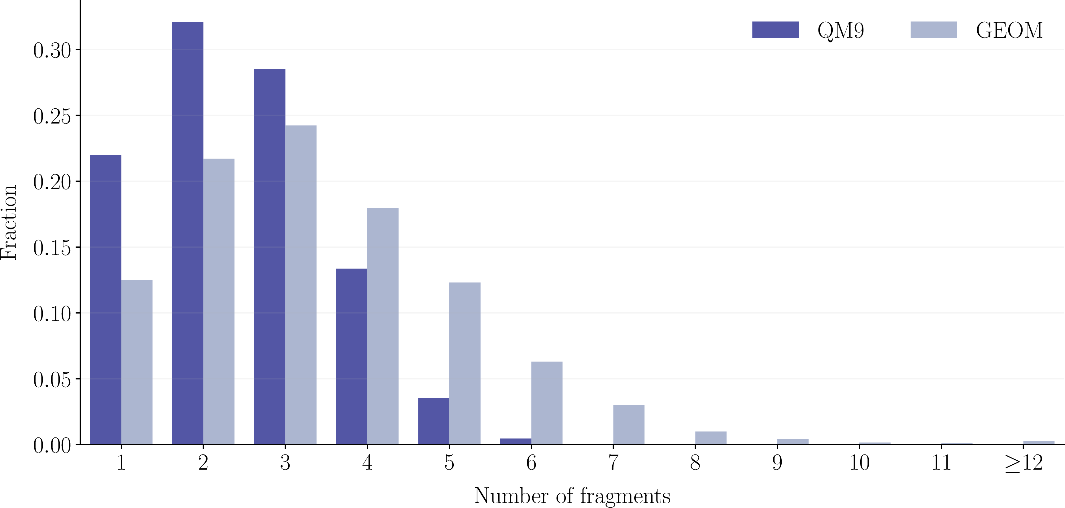
Figure 6 shows the distribution of BRICS fragment counts across molecules in QM9 and GEOM. QM9 molecules contain an average of \(2.46\) fragments (median \(=2\)), while GEOM molecules exhibit greater structural diversity, averaging \(3.40\) fragments (median \(=3\)).
8.4 Evaluation Protocol↩︎
All metrics are computed following the evaluation protocols used in prior 3D molecule generation work [3].
8.4.0.1 3D Structural Metrics.
We first evaluate generated molecules directly from their predicted 3D coordinates. 2D molecular graphs are reconstructed from atomic coordinates via distance-based bond inference [23], after which chemical validity and stability are evaluated on the reconstructed graphs.
3D Validity: fraction of generated conformations that can be converted into chemically-valid 2D molecular graphs.
3D AtomStable: fraction of atoms satisfying valence constraints under the reconstructed 2D bond order.
3D MolStable: fraction of molecules whose reconstructed 2D molecular graph satisfies chemical stability constraints.
To evaluate the geometric realism of generated molecules, we also compare local geometric statistics between generated and reference conformations. Specifically, we measure the discrepancy of bond length, bond angle, and dihedral angle distributions using Maximum Mean Discrepancy (MMD). Lower values indicate closer agreement with the reference molecular geometry distribution and therefore more realistic 3D conformations.
Bond Length: MMD between generated and reference bond length distributions for eight frequent bond types (e.g., C–C, C–N, C–O). Computed using Gaussian kernel with bandwidth tuned via the median heuristics.
Bond Angle: MMD between bond angle distributions of generated and reference molecules. Bond angles are defined over triplets of bonded atoms (e.g. C–C–C).
Dihedral Angle: MMD between dihedral (torsional) angle distributions of generated and reference molecules. Dihedral angles are defined over bonded four-atom sequences (e.g. C–C–C–C).
8.4.0.2 2D Graph Metrics
We additionally evaluate the quality of the explicitly predicted 2D molecular graph topology obtained directly from the decoder outputs, without relying on coordinate-based bond reconstruction. In this setting, validity and stability are evaluated directly on the predicted 2D molecular graphs.
2D Validity: fraction of predicted molecular graphs that satisfy chemical validity constraints.
2D AtomStable: fraction of atoms satisfying valence constraints in the predicted 2D graph topology.
2D MolStable: fraction of predicted 2D molecular graphs satisfying molecule-level chemical stability constraints.
Validity & Completeness (V&C): percentage of generated molecules that correspond to connected molecular graphs without disconnected fragments, and that can be converted into valid SMILES representations.
Validity & Uniqueness (V&U): percentage of chemically valid generated molecules that are unique under canonical SMILES comparison.
Validity & Uniqueness & Novelty (V&U&N): percentage of generated molecules that are simultaneously chemically valid, unique, and absent from the training set under canonical SMILES comparison.
V&C, V&U, V&U&N are evaluated only on directly predicted 2D molecular graphs, since uniqueness and novelty are defined with respect to 2D molecular identity (atom and bond topology). Different 3D conformations of the same 2D molecular graph are therefore not considered distinct or novel molecules.
8.5 2D molecule generation↩︎
Because KRONOS operates in the unified latent space of the UAE, generated latent tokens can be decoded into both 3D molecular structures and explicit 2D molecular graphs (utilizing predicted bond topology). This enables evaluation of the corresponding 2D molecules and direct comparison with prior methods operating on mixed 2D/3D molecular representations [2], [5], [14]. Results are reported in Table 4. Overall, KRONOS achieves competitive 2D generation performance across both benchmarks. While SemlaFlow attains the strongest overall 2D metrics, KRONOS consistently generates highly valid and stable molecular graphs, demonstrating that the proposed latent autoregressive formulation preserves the quality of the underlying discrete graph topology. These findings indicate that the proposed latent autoregressive diffusion process preserves the global information encoded in the latent representation, enabling high-quality generation in both 2D and 3D molecular modalities.
| Model | 2D Validity (\(\uparrow\)) | 2D AtomStable (\(\uparrow\)) | 2D MolStable (\(\uparrow\)) | V&C (\(\uparrow\)) | V&U (\(\uparrow\)) | V&U&N (\(\uparrow\)) | |
| (%) | (%) | (%) | (%) | (%) | (%) | ||
| QM9 | \(100.0\phantom{_{\pm 0.0}}\) | \(100.00\phantom{_{\pm 0.00}}\) | \(100.00\phantom{_{\pm 0.00}}\) | \(100.0\phantom{_{\pm 0.0}}\) | \(99.9\phantom{_{\pm 0.0}}\) | \(99.9\phantom{_{\pm 0.0}}\) | |
| Diffusion / Flow | |||||||
| JODO* | \(98.1\phantom{_{\pm 0.0}}\) | \(99.83\phantom{_{\pm 0.00}}\) | \(97.83\phantom{_{\pm 0.00}}\) | \(98.1\phantom{_{\pm 0.0}}\) | \(\mathbf{95.1}\phantom{_{\pm 0.0}}\) | \(\mathbf{95.1}\phantom{_{\pm 0.0}}\) | |
| MiDi** | \(96.8_{\pm0.1}\) | \(99.74_{\pm0.01}\) | \(96.33_{\pm0.13}\) | \(96.7_{\pm0.1}\) | \(94.4_{\pm0.1}\) | \(94.3_{\pm0.1}\) | |
| SemlaFlow** | \(\mathbf{99.4}_{\pm0.1}\) | \(\mathbf{100.00}_{\pm0.00}\) | \(\mathbf{99.63}_{\pm0.06}\) | \(\mathbf{99.3}_{\pm0.1}\) | \(\underline{94.8}_{\pm0.1}\) | \(\underline{94.8}_{\pm0.1}\) | |
| Autoregressive | |||||||
| KRONOS (ours) | \(\underline{99.2}_{\pm 0.2}\) | \(\underline{99.92}_{\pm 0.02}\) | \(\underline{99.10}_{\pm 0.02}\) | \(\underline{99.1}_{\pm 0.2}\) | \(92.5_{\pm 0.6}\) | \(92.5_{\pm 0.6}\) | |
| GEOM | \(89.4\phantom{_{\pm 0.0}}\) | \(99.44\phantom{_{\pm 0.00}}\) | \(86.27\phantom{_{\pm 0.00}}\) | \(89.4\phantom{_{\pm 0.0}}\) | \(18.5\phantom{_{\pm 0.0}}\) | \(18.5\phantom{_{\pm 0.0}}\) | |
| Diffusion / Flow | |||||||
| JODO* | \(79.1\phantom{_{\pm 0.0}}\) | \(\underline{99.26}\phantom{_{\pm 0.00}}\) | \(80.39\phantom{_{\pm 0.00}}\) | \(75.6\phantom{_{\pm 0.0}}\) | \(78.1\phantom{_{\pm 0.0}}\) | \(78.1\phantom{_{\pm 0.0}}\) | |
| MiDi** | \(59.9_{\pm0.2}\) | \(96.43_{\pm0.11}\) | \(72.85_{\pm0.32}\) | \(57.9_{\pm0.2}\) | \(59.9_{\pm0.2}\) | \(59.9_{\pm0.2}\) | |
| SemlaFlow** | \(\mathbf{95.1}_{\pm0.1}\) | \(\mathbf{100.00}_{\pm0.00}\) | \(\mathbf{98.63}_{\pm0.11}\) | \(\mathbf{92.4}_{\pm0.2}\) | \(\mathbf{95.1}_{\pm0.2}\) | \(\mathbf{95.1}_{\pm0.2}\) | |
| Autoregressive | |||||||
| KRONOS (ours) | \(\underline{84.6}_{\pm 0.4}\) | \(99.16_{\pm 0.02}\) | \(\underline{83.45}_{\pm 0.29}\) | \(\underline{84.4}_{\pm0.4}\) | \(\underline{84.5}_{\pm0.5}\) | \(\underline{84.5}_{\pm0.5}\) | |
8.6 Scaling ablations↩︎
Tables 5 and 6 evaluate the effect of scaling the transformer backbone while keeping the diffusion head fixed at dimension \(1536\). We vary the number of layers, attention heads, and hidden dimension. Across both QM9 and GEOM-Drugs, increasing model capacity consistently improves or maintains generation performance.
| Transformer heads | Transformer layers | Transformer dimension | Model parameters \((\times 10^6)\) | 3D Validity | 3D AtomStable | 3D MolStable |
|---|---|---|---|---|---|---|
| \(8\) | \(8\) | \(512\) | \(105.27\) | \(95.17_{\pm 0.04}\) | \(98.55_{\pm 0.01}\) | \(88.7_{\pm 0.2}\) |
| \(10\) | \(10\) | \(640\) | \(129.61\) | \(\underline{95.90}_{\pm 0.11}\) | \(98.67_{\pm 0.04}\) | \(89.5_{\pm 0.3}\) |
| \(12\) | \(12\) | \(768\) | \(165.78\) | \(95.87_{\pm 0.08}\) | \(\underline{98.73}_{\pm 0.01}\) | \(\underline{90.1}_{\pm 0.1}\) |
| \(16\) | \(16\) | \(1024\) | \(283.05\) | \(\mathbf{97.29}_{\pm 0.13}\) | \(\mathbf{99.07}_{\pm 0.02}\) | \(\mathbf{92.6}_{\pm 0.1}\) |
4pt
| Transformer heads | Transformer layers | Transformer dimension | Model parameters \((\times 10^6)\) | 3D Validity | 3D AtomStable | 3D MolStable |
|---|---|---|---|---|---|---|
| \(8\) | \(8\) | \(512\) | \(105.35\) | \(93.2_{\pm 0.1}\) | \(86.42_{\pm 0.11}\) | \(\mathbf{2.73}_{\pm 0.08}\) |
| \(10\) | \(10\) | \(640\) | \(129.71\) | \(93.1_{\pm 0.2}\) | \(86.23_{\pm 0.05}\) | \(2.69_{\pm 0.05}\) |
| \(12\) | \(12\) | \(768\) | \(165.90\) | \(\underline{93.4}_{\pm 0.2}\) | \(\underline{86.43}_{\pm 0.06}\) | \(2.64_{\pm 0.11}\) |
| \(16\) | \(16\) | \(1024\) | \(283.21\) | \(\mathbf{94.7}_{\pm 0.1}\) | \(\mathbf{86.45}_{\pm0.03}\) | \(\underline{2.71}_{\pm0.13}\) |
4pt
8.7 Effect of fragment-conditioning probability \(p_f\)↩︎
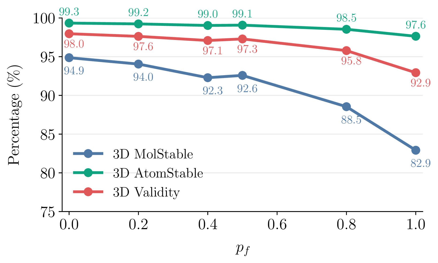
During training, each molecule is transformed to a fragment-conditioned sequence with probability \(p_f\). Figure 7 reports unconditional generation performance on QM9 as \(p_f\) varies. We observe that model’s performance on unconditional generation remains stable for moderate values of \(p_f\), with performance degrading only as training becomes dominated by fragment-conditioned examples. Based on these observations, we select \(p_f=0.5\) throughout the main experiments as a reasonable trade-off between unconditional and fragment-conditioned generation.
8.8 Generated molecule size distribution↩︎
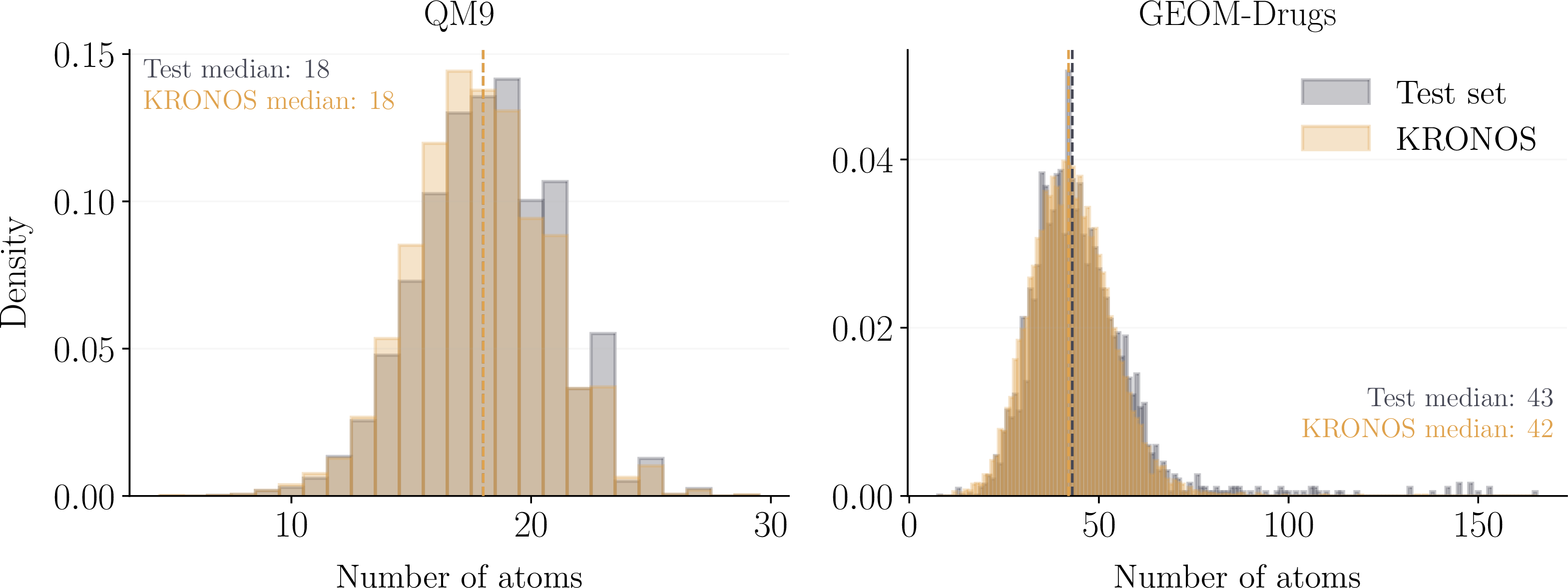
Figure 8 compares the distribution of the number of atoms in \(10\)k generated molecules against \(10\)k molecules sampled from the corresponding test sets. On QM9, the generated and test distributions exhibit identical median molecule sizes (18 atoms), while on GEOM-Drugs the generated molecules have a median of 42 atoms compared to 43 atoms in the test set. Overall, the learned stopping criterion produces molecule-size distributions that closely match those observed in the data, indicating that KRONOS effectively learns when to terminate generation.
8.9 Hyperparameters↩︎
Tables 7 and 8 report the hyperparameters used to train KRONOS on QM9 and GEOM-Drugs, respectively.
| Parameter | Value |
|---|---|
| batch size | 2048 |
| bias | false |
| dropout | 0.0 |
| epochs | 10,000 |
| diffusion head hidden dimension | 1,536 |
| diffusion head layers | 6 |
| diffusion noise schedule | cosine |
| number of diffusion steps | 100 |
| sampler | ddim |
| learning rate, weight decay | \(1.0 \times 10^{-4}\), \(10^{-6}\) |
| learning rate decay number of epochs (cosine annealing scheduling) | 10,000 |
| learning rate minimum (cosine annealing scheduling) | 10% |
| learning rate warm-up number of epochs (cosine annealing scheduling) | 50 |
| time step resampling | 4 |
| transformer heads | 16 |
| transformer hidden dimension | 1024 |
| transformer layers | 16 |
| stop classifier weight \(\lambda_{stop}\) | 1.0 |
| fragment conditioning probability \(p_f\) | 0.5 |
| Parameter | Value |
|---|---|
| batch size | 512 |
| bias | false |
| dropout | 0.0 |
| epochs | 1,000 |
| diffusion head hidden dimension | 1,536 |
| diffusion head layers | 6 |
| diffusion noise schedule | cosine |
| number of diffusion steps | 100 |
| sampler | ddim |
| learning rate, weight decay | \(1.0 \times 10^{-4}\), \(10^{-6}\) |
| learning rate decay number of epochs (cosine annealing scheduling) | 1,000 |
| learning rate minimum (cosine annealing scheduling) | 10% |
| learning rate warm-up number of epochs (cosine annealing scheduling) | 10 |
| time step resampling | 4 |
| transformer heads | 16 |
| transformer hidden dimension | 1024 |
| transformer layers | 16 |
| stop classifier weight \(\lambda_{stop}\) | 1.0 |
| fragment conditioning probability \(p_f\) | 0.5 |
8.10 Generated molecules↩︎