1 Introduction↩︎

Randomized rounding of fractional solutions is one of the most powerful and broadly applicable techniques in the design of approximation algorithms. The foundational work of Raghavan and Thompson [1] showed that independent randomized rounding of a fractional solution to a packing or covering LP, combined with Chernoff-Hoeffding concentration bounds, yields near-optimal integral solutions with high probability for a diverse set of problems. This insight sparked a long line of work on dependent randomized rounding, where the rounding procedure introduces carefully designed correlations among the rounded variables in order to enforce additional structural constraints on the output, such as matroid independence, matching feasibility, or knapsack capacity, that independent rounding cannot guarantee. Prominent examples include pipage rounding [2], swap rounding [3], dependent rounding for bipartite graphs [4], and the rounding schemes implicit in iterated rounding algorithms [5].

A particularly significant development in this line of work was the shift from designing problem-specific rounding algorithms to designing generic rounding frameworks that apply to a family of problems. The contention resolution scheme (CRS) framework introduced by Chekuri, Vondrák and Zenklusen [6], applies to rounding a polytope \(P \subseteq [0, 1]^N\) which is the independence polytope of a down-closed family of subsets \(\mathcal{I} \subseteq 2^N\).

CRS underlie state-of-the-art approximation results for many “packing” problems involving submodular maximization under matroid and knapsack constraints [6], prophet inequalities and Bayesian mechanism design [7], [8], constrained posted pricing mechanisms [7], and stochastic probing [9], [10]. The CRS framework has also been extended to other settings, in particular to online [7] and random-order [10] settings. The quality of a CRS is generally measured by its balance.

Intuitively, a CRS being balanced means that if \(x\) is not near the upper boundary of \(P\) and \(A\) is randomly selected using the probabilities from \(x\), then each element of \(A\) survives \(\pi\)’s pruning with constant probability.

1.1 Current Limits to the Applicability of CRS↩︎

One generally cannot use the algorithmic techniques in the CRS literature to obtain approximation results for problems that contain covering constraints, which of course are ubiquitous. The reason for this is that essentially all of the analyses of CRS in the literature only provides lower bounds on the expectation. So for example, [6] shows that for any non-negative linear objective function \(f(y) = \sum_{e} a_e y_e\), a \((b,c)\)-balanced CRS outputs a set \(S\) where \(\mathbb{E}[f(S)] \geq c \cdot f(x)\); as a consequence \(\mathbb{E}[|S|] \geq c \cdot \sum_{i=1}^n x_i\).

The algorithm analyses in the CRS literature that provide concentration guarantees are quite limited. Bounding the upper tail, the probability that \(f(S)\) is greater than some value, can be done by a Chernoff-type bound by appealing to the fact that \(R(\mathbf{x})\) is formed by independent sampling, and the fact that the CRS prunes \(R(\mathbf{x})\). Lower tail bounds, the probability that \(f(S)\) is less than some value, are more problematic, and there is essentially one such result in the literature. When there is a single matroid, and the linear function \(f\) is just a count of the total number of elements in the output set \(S\), the lower tail can be bounded by a Chernoff-type bound by noting that the CRS scheme of [11] always outputs a set of size equal to the rank of \(R(\mathbf{x})\), and using the concentration theorem of [3] that applies to submodular functions over the (unpruned) random set \(R(\mathbf{x})\).

As a simple illustrative example of the need for lower tail bounds in problems that arise when trying to apply a CRS to problems that involve covering constraints, let us consider the following problem. ⁵

1.1.0.1 Representative Subhypergraph Problem:

The input is a \(k\)-uniform \(k\)-partite hypergraph \(H = (V, E)\), and parameters \(\alpha \le \beta < 1\). A feasible solution is a subhypergraph \(H' = (V, E')\) of \(H\) with the property that for all vertices \(v\) the degree of \(v\) in \(H'\) lies between \(\alpha d(v)\) and \(\beta d(v)\).

Note that the natural feasibility constraints for this problem can be viewed as consisting of \(k\) collections of partition matroid constraints (one for each part) that in aggregate enforce the upper bounds on the vertex degrees, and a collection of covering constraints (one for each vertex) that in aggregate enforce the lower bounds on the vertex degrees.

The natural way to obtain a result for this problem using a CRS would be to obtain a concentration bound on the number of hyperedges selected from the collection \(E(v)\) of hyperedges containing each vertex \(v\). As noted earlier, obtaining upper tail bounds is straightforward; the lower tail bounds are the issue. The first difficulty that one runs into when trying to prove a lower tail bound is that the known CRS introduce seemingly subtle probabilistic dependencies on the selection of various elements. Further these correlations may not be negative, meaning that standard Chernoff-type bounds are apparently not applicable. In fact, negative correlations are not known for any CRS in the literature, and there is no apparent structural reason to expect them. This is further complicated by the fact that we need concentration bounds for all subsets of the form \(E(v)\), and the elements selected in \(E(v)\) may be largely determined by random events associated with hyperedges not in \(E(v)\).

Thus the natural research question that we consider is:

By the discussion above, this reduces to a concrete technical question about the output of a CRS: is there a contention resolution scheme for the intersection of \(k\) matroids whose output \(S\) concentrates from below on every target set \(T\) (in our example, the sets \(E(v)\) of hyperedges incident to each vertex \(v\))? That is, for which \(|S \cap T|\) attains a constant fraction of \(\sum_{e \in T} x_e\) with high probability, for every \(T\)?

1.2 Our Results↩︎

Our main contribution is the first lower tail concentration bound for a CRS. In particular, we prove a lower tail concentration for the random-order CRS of Adamczyk and Włodarczyk [10], which we call AW. In fact, we prove the stronger result that concentration holds for any linear function with coefficients in \([0,1]\). Note that taking \(a_e = 1\) for \(e \in T\) for some subset \(T\), and \(a_e=0\) otherwise, yields a lower tail bound concentration result for the subset of elements \(T\).

Several features of this bound deserve emphasis. The bound is dimension-free: the failure probability depends only on \(Q\), \(k\), and \(\delta\), but not on \(n = |U|\), the size of the ground set. This mirrors the dimension-free concentration bounds of swap rounding [3] and is essential for applications where \(Q\) may be much smaller than \(n\). The bound is meaningful and strong when \(Q \gg k^3\): the failure probability decays exponentially in \(\delta^2 Q/k^3\), so for any fixed \(k\) the bound becomes exponentially strong as \(Q\) grows.

Note that Theorem 1 only bounds the probability of falling below \(\frac{Q}{5(k+1)}\), a factor of \(5\) smaller than the expectation bound of \(\frac{Q}{k+1}\) proven in [10]; that is, the output attains a constant fraction, rather than all, of its expectation with high probability. This was necessitated by the fact that our analysis only applies to a prefix of the elements in the random ordering used by the AW algorithm, as the dependencies affecting the later elements become too large. As we shall see, for many covering applications this is sufficient.

1.3 Applications of Theorem 1↩︎

Given the ubiquity of covering constraints, we expect that extending CRS to problems with both packing and covering constraints should significantly broaden their reach. To support this expectation, we apply Theorem 1 to several natural problems involving both packing and covering constraints. To make this more accessible on a first read, we largely omit background definitions, and only state the results informally. Background definitions and formal statements of the results can be found in the later technical sections.

1.3.0.1 Matroid Intersection Coloring.

An instance of this problem consists of \(k\) matroids \(M_1, \ldots, M_k\) on a common ground set \(U\). A feasible solution is a partition of \(U\) into parts that are each independent in all matroids. The objective is to minimize the number of parts. The problem is NP-Hard, even for two matroids [12], [13]. There are non-constructive existential results using topological fixed-point arguments [14]–[16], and there are approximation algorithms, some for special types of matroids [17]–[20]. The best previously known approximation ratio for \(k\) general matroids was \(O(k^2)\) [21]. Theorem 1 yields the following improvement to the best known achievable approximation ratio when the optimal objective value is sufficiently large.

1.3.0.2 Monotone Submodular Maximization with Matroid, Packing, and Covering Constraints.

An instance of this problem consists of a monotone submodular function \(f\) on a ground set \(U\), \(k\) matroids on \(U\), packing constraints, and covering constraints. A feasible solution is a subset of \(U\) that is independent in all of the matroids, and satisfies the packing and covering constraints. The objective is to maximize \(f\). Monotone submodular maximization is a well-studied optimization problem receiving considerable attention over the past few decades [22]–[25]. Under a single matroid constraint, the problem admits an optimal polynomial-time \((1-1/e)\)-approximation via a continuous greedy algorithm, and pipage rounding or swap rounding [24]. Under a single matroid constraint and a constant number of packing and covering constraints, the problem also admits an optimal polynomial-time \((1-1/e-\varepsilon)\)-approximation for all fixed \(\varepsilon> 0\), allowing violation of the covering constraints by a factor of \(1-\varepsilon\) [26]. Under the intersection of \(k\) matroid constraints, but no packing and covering constraints, the best known polynomial-time approximation guarantee is \(\frac{1}{k+\varepsilon}\) for every fixed \(\varepsilon> 0\) [25], and the standard greedy algorithm gives a \(\frac{1}{k+1}\)-approximation [22].

As in [6], we work in what they called the “loose constraints” setting. When all constraints are normalized so that the left-hand-side coefficients are in \([0,1]\), define the capacity of an instance to be the minimum right-hand-side value over the \(p\) packing constraints, and the width of a covering instance to be the minimum right-hand-side value over the \(c\) covering constraints. Theorem 1 yields a bicriteria approximation result for monotone submodular maximization under \(k\) matroid constraints, packing constraints with logarithmic capacity, and covering constraints with logarithmic width.

As far as we know, this is the first approximation algorithm for monotone submodular maximization in the setting of \(k\) matroid constraints, packing constraints, and covering constraints. As we shall explain later, the \(O(k)\) violation of the covering constraints is essentially best possible provided \(NP \not \subseteq BPP\).

Applying this result to the Representative Subhypergraph problem from the introduction yields a randomized polynomial-time algorithm that, on instances where there is a feasible solution, and where the lower degree bounds are logarithmic, outputs a subhypergraph \(H'\) that satisfies the upper degree bounds, and that violates the lower degree bounds by at most an \(O(k)\) factor (Appendix 6). ⁶

1.4 Technical Overview↩︎

Here we provide an overview of the proof of our main result in Theorem 1.

1.4.0.1 The CRS AW:

Let us first describe the scheme for a single matroid \(M\). The input is a point \(\mathbf{x}\) in the independence polytope \(P(M)\) of \(M=(U, {\mathcal{I}})\). Initially, the scheme decomposes \(\mathbf{x}\) into a convex combination \(\mathbf{x} = \sum_{i} \beta_i \mathbf{1}_{I_i}\) of incidence vectors of independent sets \(I_i\) of \(M\). The scheme maintains a mapping \(\phi_{ij}\) between each pair of independent sets \(I_i\) and \(I_j\), that we call exchange mappings, with the property that \(I_j - \{\phi_{ij}(e) \} \cup \{e\}\) is independent for all \(i, j\) and elements \(e \in I_i\). These independent sets and exchange mappings are updated as the scheme executes. For each element \(e\), the scheme selects a random independent set \(I_i\) containing \(e\) as its “controller.” The scheme then generates the random set \(R(\mathbf{x})\), (here it is more convenient here to think of this being done internally to the scheme), and considers the elements in \(R(\mathbf{x})\) in a random order \(\sigma\).

When an element \(e\) is being considered, it is added to the output set \(S\) if and only if \(e \in R(x)\) and \(e\) is still a member of its controller independent set \(I_i\). If \(e\) is added to \(S\) then each independent set \(I_j\) is updated by adding \(e\) and deleting \(\phi_{ij}(e)\). These independent set updates may cause an element \(f=\phi_{ij}(e)\) to be kicked out of its controller \(I_j\), and thus killing \(f\)’s chances of being added to \(S\) later. For multiple matroids, the single matroid algorithm is run for each matroid, and the final output is just the intersection of the \(S\)’s for the individual matroids.

1.4.0.2 Sequential Selection Process.

In our analysis we abstract away the matroid structure and the CRS entirely, and analyze a general object that we call a sequential selection process. The process starts with a ground set \(U\) and an arbitrary point \(\mathbf{x} \in [0, 1]^U\). The process considers the elements of \(U\) in a uniformly random order. The process initializes a residual vector \(\mathbf{p}\) to be \(\mathbf{x}\), and updates \(\mathbf{p}\) over time. Let \(\mathbf{p}(t)\) be the value of this residual vector right before the \(t^{th}\) element is considered. When an element \(e\) is considered at step \(t\), it is selected into the output only if \(e \in R\), and in that case with probability at least \(p_e(t)/x_e\); hence unconditionally, \(e\) is selected with probability at least \(p_e(t)\). After this step, the entries in the residual vector are decreased in some arbitrary way. We write \(\mathbf{X}\) for the \(\{0,1\}\) characteristic vector of the output. The CRS of [10] is a special case of this process, so any lower tail bound we prove for the abstract process applies to it.

1.4.0.3 Strong \(\lambda\)-boundedness.

The main technical difficulty in obtaining lower tail concentration bounds for a sequential selection process is that it is adversarial: the drops \(\mathbf{\Delta}(t) := \mathbf{p}(t) - \mathbf{p}(t+1)\) are chosen adaptively, so the acceptance probabilities are history-dependent and the correlations among selections are neither negative nor otherwise structured. This rules out Chernoff bounds, negative association, and the submodular concentration result of [3]. Our first contribution is thus definitional: identifying the property of a sequential selection process that makes concentration possible. Adamczyk and Włodarczyk [10] showed that in their CRS AW it is the case that any fixed element can be killed only by a set of elements with total fractional mass in \(\mathbf{x}\) of at most \(\lambda\), where \(\lambda = 1\) for a single matroid and \(\lambda = k\) for \(k\) matroids. We will call this property \(\lambda\)-boundedness. ⁷ The property of \(\lambda\)-boundedness sufficed for the expectation guarantee achieved in [10], but provably is not sufficient to imply the sort of concentration result we seek for a sequential selection process. The issue is that the fractional mass which kills each element could heavily overlap, so \(\lambda\)-boundedness does not provide any worst-case control on the aggregate decrease to the components of the residual vector \(\mathbf{p}\). The danger is that an element considered early in the random order could zero out most components in \(\mathbf{p}\), and if this happens with some decent probability, then concentration is unachievable.

Our key insight is that the CRS AW has a stronger property, that we will call \(\lambda\)-limitedness, which limits the amount of decrease that a single element can cause in aggregate to the entries of the residual vector \(\mathbf{p}\). A sequential selection process is \(\lambda\)-limited if at every step, the 1-norm decrease to the residual vector, namely \(\|\mathbf{p}(t) - \mathbf{p}(t+1)\|_1\), is at most \(\lambda\). Intuitively, this says each accepted element kills at most \(\lambda\) fractional mass in total, ruling out the dangerous case above. The two properties of \(\lambda\)-boundedness and \(\lambda\)-limitedness are now symmetric. Each element is killed by at most \(\lambda\) fractional mass and kills at most \(\lambda\) fractional mass. We show that one can obtain concentration results for every sequential selection process that is strongly \(\lambda\)-bounded, which we define to be both \(\lambda\)-bounded and \(\lambda\)-limited.

1.4.0.4 Our three-step chaining argument.

We give a three-step argument to show that the strong \(\lambda\)-boundedness of a CRS implies the concentration bounds in Theorem 1. At a high level our analysis of a strongly \(\lambda\)-bounded sequential selection process shows that the first \(m=\Theta(n/\lambda)\) elements in the random order behave almost like an independent rounding of the input vector \(\mathbf{x}\). We show that the output set \(S\) well approximates the input vector \(\mathbf{x}\) using intermediate vector \(\mathbf{q}\), where \(q_e\) is the probability that element \(e\) is accepted when it is considered in the sequential selection process. Our analysis consists of three steps, and is illustrated by the following diagram: \[\overline{\mathbf{a}}(m)\cdot\mathbf{X} \;\xrightarrow[]{\text{Step 1}}\; \overline{\mathbf{a}}(m)\cdot\mathbf{q} \;\xrightarrow[]{\text{Step 2}}\; \overline{\mathbf{a}}(m)\cdot\mathbf{x} \;\xrightarrow[]{\text{Step 3}}\; \tfrac{m}{n}\, \mathbf{a}\cdot\mathbf{x},\] where \(\overline{\mathbf{a}}(m)\) zeros out the elements in \(\mathbf{a}\) that are not in the first \(m\) positions of the random order. Each arrow represents a high-probability lower bound (up to lower-order slack) on the left-hand quantity in terms of the right. Chaining the three steps and using \(\mathbf{a}\cdot\mathbf{X} \ge \overline{\mathbf{a}}(m)\cdot\mathbf{X}\) completes the argument.

Step 1: Conditioned on the history, each element’s inclusion in \(S\) is a coin flip with bias \(q_e\), but note that the value of \(q_e\) depends heavily on the history. The claim then follows by the application of Freedman’s martingale inequality, which tolerates history-dependent biases.

Step 2: This is the key step, and the only step that uses \(\lambda\)-limitedness and \(\lambda\)-boundedness. Since \(q_e\) is lower-bounded by the residual weight \(p_e\) at the moment \(e\) is processed, it suffices to show that, on average, residual weights have not decayed far from their initial values \(x_e\) over the prefix.

The proof of this step requires finding the right potential function to effectively apply Freedman’s inequality. We track \(\overline{\mathbf{a}}(m)\cdot \mathbf{p}(t)/(n-t+1)\). This potential’s expected change per step is the difference of two terms, a gain of order \(\overline{\mathbf{a}}(m)\cdot \mathbf{x}/(n-t)^2\) from the shrinking denominator as \(t\) increases, and a loss of order at most \(\lambda\, \overline{\mathbf{a}}(m)\cdot \mathbf{x}/(n-t)^2\) due to \(\lambda\)-boundedness. These effects are lower-order terms with respect to this potential, and since the increments we analyze are differences of consecutive values of this potential, the overall sum telescopes to a comparison of the initial potential \(\overline{\mathbf{a}}(m)\cdot \mathbf{x}/n\) against the final one, which yields the comparison between \(\mathbf{x}\) and \(\mathbf{q}\) that this step requires. Freedman’s inequality then applies, with \(\lambda\)-boundedness controlling the expected increments and \(\lambda\)-limitedness their worst case. Each step’s drift is a \(\lambda/n\) fraction of the potential’s initial value, so the drift budget is exhausted after \(\Theta(n/\lambda)\) steps; this is what dictates the prefix length \(m\).

Step 3: This step only uses the fact that the first \(m\) elements in a uniformly random order are a uniformly random sample of size \(m\), and hence negatively associated. The step then follows by a standard Chernoff bound for sampling without replacement.

1.5 Organization↩︎

2 reviews the main concentration inequalities used in our proof of Theorem 1. 3 shows that the CRS AW is a strongly \(k\)-bounded sequential selection process for \(k\) matroids, and proves 1. 4 applies 1 to matroid intersection coloring, proving 2. 5 applies 1 to monotone submodular maximization under matroid, packing, and covering constraints, and proves 3.

2 Concentration Inequalities↩︎

We now state a some known concentration inequalities that will be useful for our proofs, in particular, Freedman’s inequality [27], Bhatia-Davis’ inequality [28],⁸ and Bernstein’s inequality [29], [30]. Freedman’s inequality is the main workhorse for obtaining our concentration guarantees.

Note that as long as \(|X_t| \leq c\) for some value \(c > 0\), we can rescale and center the \(X_t\)’s to apply Freedman’s Inequality. Further, it is often useful to identify an absolute upper bound \(B\) on the total quadratic variation \(T_n = \sum_{t=1}^n V_t\), so that the condition \(T_n \leq B\) can be dropped from the probability statement and give a concentration guarantee just involving the sum \(S_n\). Thus the “recipe” for applying Freedman’s inequality is often to identify these two absolute upper bounds \(c, B > 0\), with the goal of minimizing them because larger values of \(c, B\) degrade the concentration guarantee.

The Bhatia-Davis Inequality will be useful in our “recipe” for Freedman’s Inequality because it will allow us to produce an absolute upper bound \(B\) on the total quadratic variation \(T_n\) by only using the bounds and mean of each random variable \(X_t\).

7 follows from Bernstein’s inequality ([thm:bernstein]) and Hoeffding’s comparison theorem [30]. Bernstein’s inequality gives the above statement if \(T\) is sampled independently with replacement, i.e. \(T\) is a collection of \(m\) independent uniform random values of \(S\). Hoeffding’s comparison theorem [30] allows us to transfer Bernstein-style concentration bounds from the with replacement setting to the without replacement setting.

3 Sequential Selection Process↩︎

In 3.1, we formally define a sequential selection process and related properties. We then show that sequential selection processes compose in the same way that CRS do. In 3.2, we show that the \(k\)-matroid AW algorithm is a strongly \(k\)-bounded sequential selection process. In 3.3, we analyze the concentration properties of strongly \(\lambda\)-bounded sequential selection processes, and prove 1.

3.1 Definition and Notation↩︎

The purpose of this subsection is to define a sequential selection process, and related terms, and show in Lemma 1 that sequential selection processes compose in the same way as CRS.

3.2 Analysis: AW Algorithm and Sequential Selection Process↩︎

In this section, our ultimate goal is to prove 3, which states that the \(k\)-matroid AW algorithm is a strongly \(k\)-bounded sequential selection process. We begin by giving a complete description of the AW CRS for a single matroid. We then show in 2 that the single-matroid AW CRS is a strongly \(1\)-bounded sequential selection process. Then, in 3, we show that the \(k\)-matroid AW CRS is a strongly \(k\)-bounded sequential selection process, which follows from 1 and 2. We first need the following standard definition of an exchange mapping between pairs of independent sets in a matroid.

That exchange maps exist and can be constructed efficiently follows from standard matroid results (see Schrijver Corollary 39.12a [31]). We now describe the AW CRS for a single matroid.

Having shown the AW CRS is strongly 1-bounded for a single matroid, we can now leverage 1 to show that the \(k\)-matroid AW CRS yields a strongly \(k\)-bounded sequential selection process. To obtain this, note that the \(k\)-matroid AW CRS is defined by simply running the AW CRS for each matroid individually to obtain sets \(S_j \subseteq U\) such that \(S_j\) is independent in \(M_j\), and then outputting their intersection \(S\) which is independent in all matroids. The only nuance is that when running the individual CRS’s, we share the same random order on \(U\) and random set \(R\) [10]. This yields:

3.3 Analysis: Concentration of Sequential Selection Process↩︎

In this section, our ultimate goal is to prove our main technical theorem, 8, which shows dimension-free concentration properties of strongly \(\lambda\)-bounded sequential selection processes.

8 immediately yields our main theorem, 1, because the \(k\)-matroid AW algorithm is a strongly \(k\)-bounded sequential selection process (3) with output \(S = \{e \in U : X_e = 1\}\).

To show 8, we focus on the first \(\Theta(1/\lambda)\) fraction of the elements in the random order \(\sigma\), as the accumulated drift beyond this prefix becomes unmanageable (see 1.4). Formally, for an integer \(m \in [0, n]\), we define \(\overline{\mathbf{a}}(m)\) by \(\overline{a}_e(m) = a_e\) if \(\sigma^{-1}(e) \leq m\) and \(\overline{a}_e(m) = 0\) otherwise. We then apply the three step process, described in 1.4, in 3.3.1, 3.3.2 and 3.3.3. The analyses of these steps are essentially logically independent (although our exposition of the later steps may rely on definitions introduced in the earlier steps). In 3.3.4 we combine the results of each of these three steps to prove 8.

3.3.1 Step 1↩︎

In 4, we show that \(\overline{\mathbf{a}}(m) \cdot \mathbf{X}\) is not much smaller than \(\overline{\mathbf{a}}(m) \cdot \mathbf{q}\) with high probability, where for each \(e \in U\) we define \(q_e = \Pr[X_e = 1 \mid \mathcal{F}_{t-1}, e = \sigma(t)]\) with \(t = \sigma^{-1}(e)\). In other words, \(q_e\) is the actual probability that \(X_e\) is set to \(1\) at the time that \(e\) is processed. Note that \(q_e \geq x_e \cdot \frac{p_e(t)}{x_e} = p_e(t)\) for \(t = \sigma^{-1}(e)\).

3.3.2 Step 2↩︎

The main result of this step is 7, where we show that \(\overline{\mathbf{a}}(m) \cdot \mathbf{q}\) is at least a constant fraction of \(\overline{\mathbf{a}}(m) \cdot \mathbf{x}\) with high probability (when \(m = O(n/\lambda)\)). 7 is the key technical lemma where we use the two properties of strong \(\lambda\)-boundedness.

First, in 5, we define the random variable \(Z_t\), which is the key underlying random variable for relating \(\overline{\mathbf{a}}(m) \cdot \mathbf{q}\) to a constant fraction of \(\overline{\mathbf{a}}(m) \cdot \mathbf{x}\). Conceptually, \(Z_t\) encodes the per-step change in the normalized potential \(\overline{\mathbf{a}}(m) \cdot \mathbf{p}(t)/(n-t+1)\) introduced in 1.4, shifted by a small deterministic compensator; strong \(\lambda\)-boundedness guarantees that this change is small with high probability. We then shift and rescale \(Z_t\) to a random variable \(W_t\) satisfying the preconditions of Freedman’s inequality (6). Finally, we apply Freedman’s inequality to \(W_t\) to prove 7.

Next, we define the random variable \(W_t\), which is the shifted and rescaled version of \(Z_t\) that satisfies the preconditions of Freedman’s inequality.

Next, we apply Freedman’s inequality to the \(W_t\) random variables to prove 7.

3.3.3 Step 3↩︎

In 8, we show that \(\overline{\mathbf{a}}(m) \cdot \mathbf{x}\) is close to \(\frac{m}{n} \, \mathbf{a} \cdot \mathbf{x}\) with high probability.

3.3.4 Combining the Steps↩︎

We combine the results of our three steps, given in 4, 7, and 8, to lower bound \(\overline{\mathbf{a}}(m) \cdot \mathbf{X}\) (and thus \(\mathbf{a} \cdot \mathbf{X}\)) by a constant fraction of \(\mathbf{a} \cdot \mathbf{x}\) with high probability (9). We then choose \(m = \Theta(n/\lambda)\) to complete the proof of 8.

Lastly, we approximately optimize and clean the statement in 9 to prove our main technical theorem (8).

Finally, 1 follows immediately from 8 and 3 and the fact that the output of the \(k\)-matroid AW algorithm is \(S = \{e \in U : X_e = 1\}\).

4 Application to Matroid Intersection Coloring↩︎

In this section, we show to apply 1 to obtain an improved approximation algorithm for the simultaneous coloring of several matroids, proving 2.

Suppose \(M_1, \dots, M_k\) are matroids on a common ground set \(U\) with \(|U| = n\), each with chromatic number \(\chi(M_j)\), let \(\chi_{\max}:= \max_{j \in [k]} \chi(M_j)\), and let \(M_{\mathsf{int}}:= \bigcap_{j\in[k]} M_j\). The matroid intersection coloring problem asks for a partition of \(U\) into the fewest color classes, each of which is a common independent set of \(M_1, \dots, M_k\); the minimum number of colors required is \(\chi(M_{\mathsf{int}})\). Since every color class must be independent in each \(M_j\) individually, we have \(\chi(M_{\mathsf{int}}) \ge \chi_{\max}\), so \(\chi_{\max}\) is a natural lower bound and the approximation ratio is frequently measured against it.

The best previously known approximation ratio for \(k\) general matroids is \(O(k^2)\), due to Arndt, Moseley, Pruhs, Swamy, and Zlatin [21]. That work gives two algorithms. The first is an unconditional \(k(k-1)\)-approximation for all \(k\), which we state formally here as we invoke it in our algorithm.

The second algorithm of [21] achieves a \((1+\varepsilon)\)-approximation when \(\chi_{\max}\) is sufficiently large, but is restricted to \(k = 2\) matroids using a concentration result on swap rounding. We follow a similar algorithmic framework, employing our concentration result on \(k\) matroids to obtain the following, which is a formal version of 2.

4.1 Overview of the Matroid Intersection Coloring Algorithm and its Analysis↩︎

The chromatic number of a single matroid is governed by its sets of high density: namely subsets \(S\) for which the ratio \(|S|/r(S)\) of cardinality to rank is large. In particular, Edmonds gave an explicit formula for the chromatic number of a single matroid \(M\) on ground set \(U\): \[\chi(M) = \max_{S \subseteq U} \lceil |S| / r_M(S)\rceil.\] Thus, reducing the chromatic number of one matroid is therefore equivalent to breaking up all its high-density sets simultaneously. This suggests a natural covering strategy: sample a collection of independent sets common to all matroids, use them as color classes and remove their elements. If in all \(k\) matroids, the maximum density of the remaining elements drops below \(\chi_{\max}/ k\), then the unconditional \(O(k^2)\)-approximation of [21] for matroid intersection coloring can be applied to color the rest within budget.

4.1.0.1 Random Thinning

The key question then, is how to sample color classes to achieve this goal? We do this in two distinct phases: in the first phase, random thinning, we sample a random collection of \(L = O(k \log k \cdot \chi_{\max})\) common independent sets utilizing the AW CRS [10]. By definition of the chromatic number, the fractional point \(\mathbf{1}/\chi_{\max}\), lies in the matroid polytope \(P(M_j)\) for each \(j \in [k]\), and so this point is a valid input to the AW CRS. Due to our concentration bound on the output of the scheme, we can show that all subsets of sufficiently high rank (rank at least \(R = C_R \cdot k^4\) for some constant \(C_R\)) are covered to the desired extent by this collection. There are up to \(n^m\) flats of rank \(m\), so establishing this simultaneously via a union bound requires the per-flat failure probability to decay exponentially in \(m\). This is exactly where our concentration theorem is used: for a fixed flat \(F\) of rank \(m\), the theorem gives a lower-tail bound on the number of elements of \(F\) covered by a single CRS sample. Repeating this \(L=O(k\log k \cdot \chi_{\max})\) times and applying a sharp Chernoff bound to the number of bad samples yields a per-flat failure probability of \(\exp\left(-\Omega\left(\frac{m \chi_{\max}}{k^3}\right)\right) \leq n^{-\Omega(m)}\), since \(\chi_{\max}\ge Ck^3\log n\). The expectation bounds typically proven for CRS are, of course, insufficient here, as we need the high-probability guarantee on each flat in order to enact the union bound over all \(n^m\) flats of rank \(m\).

4.1.0.2 Deterministic Thinning

The random thinning phase only has the desired density reduction on flats of rank at least \(R\). To deal with the low rank sets, we enact a phase of deterministic thinning. We repeatedly extract the highest density set in each iteration, until the overall chromatic number drops to the desired threshold of at most \(\chi_{\max}/k\) in each matroid. The key observation is that the high-rank sets all have low density after Phase 1, hence the collection of extracted sets (which are high density) have rank which is at most \(R = \Theta(k^4)\). Their union has a rank which is at most \(kR = O(k^5)\) in \(M_{int}\), hence we can easily color this collection using a standard greedy algorithm for Set Cover with a \(k\)-approximate maximum coverage oracle, yielding a coloring of at most \(O(k \log k) \cdot\)OPT sets.

4.1.0.3 Coloring the Remainder

After the thinning of Phases 1 and 2, the final residual set has a maximum chromatic number at most \(\chi_{\max}/ k\) and we can apply the \(O(k^2)\) approximation of 9 to the residual ground set to obtain the desired final coloring.

4.2 Algorithm For Matroid Intersection Coloring↩︎

We now present the main algorithm.

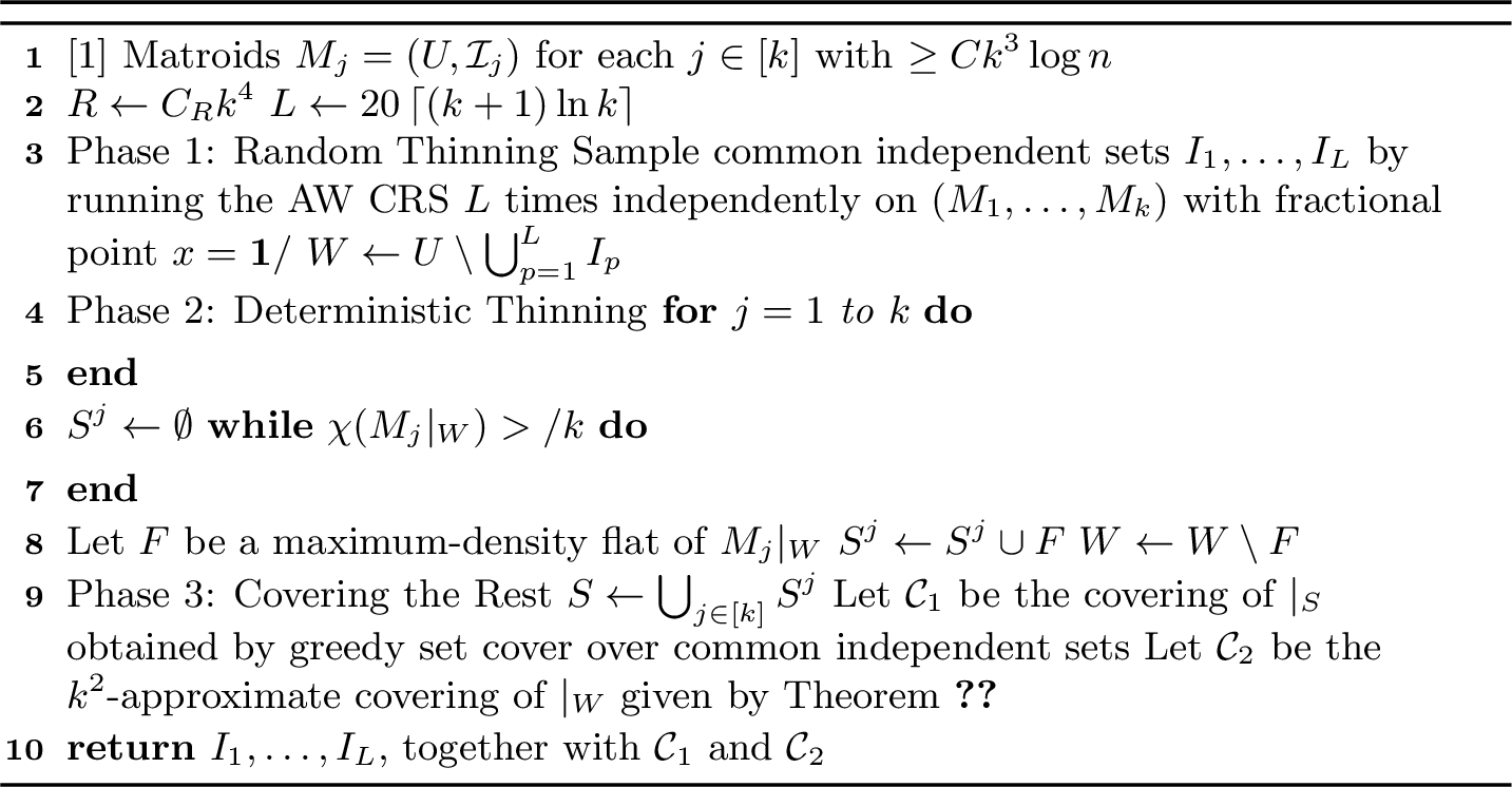
1 proceeds in three phases. The first phase uses the AW CRS (or any Contention Resolution scheme satisfying 1) to repeatedly sample common independent sets and remove the elements covered. This has the effect of reducing the density of all high-rank subsets with high probability. Then, in Phase 2, we deterministically extract subsets of highest density until all subsets have a sufficiently low density. If the high probability event of Phase 1 was successful, then after Phase 2 is complete, the chromatic number of each matroid on the residual elements \(W\) is at most \(\chi_{\max}/ k\), while the extracted high density flats form a collection \(S\) of low rank. This allows us to in Phase 3 cover the elements of \(S\) using an algorithm for Set Cover with an approximate maximum coverage oracle, and to color the elements of \(W\) using the previously known \(O(k^2)\) approximation.

4.3 Analysis of 1↩︎

We now proceed with the analysis. We begin with a relatively standard concentration bound that we will need in the coming analysis.

We now prove the first key result, which is that after Phase 1, the density of all sets with rank greater than \(R\) is at most \(\chi_{\max}/k\) with high probability. We assume \(\chi_{\max}\geq Ck^3 \log n\).

In order to prove this key claim, we first need the following technical lemma, which follows from 1.

We now turn to establishing the desired properties of Phase 2, namely that (i) the chromatic number of every matroid is reduced to \(\chi_{\max}/ k\), and (ii) the overall rank of the extracted flats is upper bounded by a polynomial in \(k\). The first property is proved in 12, which holds deterministically. Indeed, it is essentially true by construction as it defines the termination condition of Phase 2. The second property ([lem:exceptional-sets-low-rank,lem:exceptional-set-low-intersection-rank]) is satisfied whenever the good event of Phase 1 holds.

In the following lemma the notation \(r_{M_{int}}\) denotes rank function of the matroid intersection set system. So in particular, \(r_{M_{\mathsf{int}}}(A):=\max\{|I|: I\subseteq A,\;I\in \bigcap_{j=1}^k \mathcal{I}_j\}\).

14 allows us to cover \(S\) using a refined approximation for Set Cover whose approximation ratio which depends on the maximum set size. The classical greedy approximation algorithm for Set Cover achieves an approximation ratio of \(O(\log d)\) where \(d\) is the maximum cardinality of any set in the system. However, implementing the greedy algorithm for a \(k\)-matroid set system is NP-hard, so we use an approximate maximum coverage oracle. We recall the folklore result on Set Cover with an approximate maximum coverage oracle here. For example, this follows via the analysis in  [24].

To implement the maximum coverage oracle in our setting, a simple greedy algorithm will yield a \(k\)-approximate maximum cardinality set in the intersection of \(k\) matroids. One could also use the improved \((k/2+\varepsilon)\)-approximation of  [33] but this constant factor does not matter for our purposes. We are now ready to prove the overall approximation bound on the performance of 1.

We can now conclude by combining the above claims to give a proof of the main result of this section.

5 Application to Monotone Submodular Maximization↩︎

In this section, we apply 1 to obtain new guarantees for constrained monotone submodular maximization (see 3). In particular we give a polynomial-time bicriteria approximation algorithm for maximizing a monotone submodular function \(f\) subject to \(k\) matroid constraints, and \(p\) packing and \(c\) covering constraints, extending [26] which handles a single matroid and constantly many packing and covering constraints. We require the constraints to be loose: each packing constraint has a right-hand value at least \(\Omega(\log p)\) and each covering constraint has right-hand value at least \(\Omega(k^3 \log c)\). Under these conditions, we show that the continuous greedy algorithm [24] followed by the AW CRS, outputs a set \(S\) satisfying all packing constraints without any violation, and all covering constraints up to an \(O(k)\) factor, simultaneously with high probability in \(p\) and \(c\). Furthermore, the value of \(f(S)\) is a \(\left(\frac{1-1/e-\varepsilon}{k+1}\right)\)-approximation to the optimal objective. This is formally stated in 16.

5.0.0.1 Technical Overview

To obtain our result, we prove high probability bounds on the likelihood that our solution is feasible for all constraints. The packing and covering constraints are structurally different in this respect. For packing, since the AW CRS first draws a random set \(R\) by independently including each element \(e\) with probability \(\bar{x}_e\) (where \(\bar{x}\) is the fractional points returned by continuous greedy), and \(S \subseteq R\), a standard Bernstein inequality applied to \(R\) shows that each packing constraint \(\sum_{e \in S} A_{ie} \leq b_i\) is satisfied with failure probability at most \(1/(p+2)^5\), allowing a union bound over the \(p\) packing constraints to give feasibility with high probability.

For covering, each constraint \(\sum_{e \in S} C_{ie} \geq d_i\) is a lower bound on a linear function \(\mathbf{C}_i \cdot \mathbf{1}_S\) of the output, where \(\mathbf{C}_i \in [0,1]^U\) is the \(i\)-th row of covering constraint matrix \(C\). This is where our main concentration theorem is needed: 1 bounds the failure probability of each covering constraint by \(4\exp\!\bigl(-\Omega(\delta^2 d_i / k^3)\bigr)\), and by the looseness condition, we have \(d_i = \Omega(k^3 \log (c+2))\). Hence, the failure probability per covering constraint is at most \(4/(c+2)^5\), allowing a union bound over the \(c\) constraints as before.

The \(\Omega(k)\) violation of covering constraints is tight. One can encode a \(k\)-dimensional matching instance via \(k\) partition matroids and a single covering constraint on matching size; any violation below \(o(k)\) would yield an \(\frac{1}{o(k)}\)-approximation for \(k\)-dimensional matching which does not exist unless \(\text{NP} \subseteq \text{BPP}\) [34].

5.0.0.2 Organization of the Section.

In 5.1, we discuss preliminaries for our result. In 5.2, we state our main theorem and algorithm. In 5.3, we analyze the algorithm and proved the stated guarantees. In 5.4, we provide context for our result, by showing the problem becomes NP-hard upon removal of any main assumption.

5.1 Preliminaries↩︎

Our algorithm combines two existing algorithmic tools: the continuous greedy method for optimizing the multilinear extension of a submodular function, and the AW CRS for rounding fractional points in the intersection of \(k\) matroid polytopes. We recall the relevant guarantees below.

The multilinear extension \(F\) enables continuous relaxation of submodular maximization. The following theorem guarantees that it can be approximately maximized over any solvable polytope in polynomial time.

Once a near-optimal fractional point is found, the AW CRS rounds it to a feasible integral solution while preserving a \(\tfrac{1}{k+1}\) fraction of the objective. For the monotone case, every element greedily improves the objective, so the output equals the rounded set directly.

As an immediate corollary, if \(f\) is monotone submodular, then the condition \(f(X \cup \{e\}) \geq f(X)\) is always satisfied and we obtain \(X = S\).

5.2 Main Theorem and Algorithm↩︎

Algorithm: Compute a \((1-1/e-\varepsilon/2)\)-approximate solution \(\bar{x}\) to \(\max\{F(x) : x \in (1-\varepsilon/2)P\}\) where \(F(x)\) is the multilinear extension of \(f(X)\) (14). Let \(S\) be the output of the AW algorithm on matroids \(M_1, M_2, \dots, M_k\) and fractional point \(\bar{x}\). Output \(S\).

5.3 Analysis↩︎

We verify the three components of 16 separately. 16 establishes the approximation ratio. 17 shows the packing constraints are satisfied exactly with high probability. 18 shows the covering constraints are satisfied approximately with high probability, and is the step where 1 is invoked. The proof of 16 then follows by a union bound over the latter two.

The packing argument above required nothing beyond \(S \subseteq R(\bar{x})\) and independence of the elements of \(R(\bar{x})\); no matroid structure was needed. The covering argument, by contrast, invokes the concentration result of 1 directly, as discussed above.

5.4 Context for Result↩︎

We now show that each assumption in 16 is necessary in the sense that removing any single condition makes desired guarantees intractable to obtain.

5.4.0.1 Approximation Factor:

It is impossible to achieve an approximation factor of \(\frac{1}{o(k)}\), even if \(f(X) = |X|\), the matroids \(M_i, i \in [k]\) are partition matroids, and there are no packing and covering constraints provided \(NP \not \subseteq BPP\), as this captures the \(k\)-dimensional matching problem [34].

5.4.0.2 Packing Constraints:

We must add some assumption on the packing constraints, as otherwise \(f(X) = |X|\) and the packing constraints alone can encode the maximum independent set problem in graphs, which is NP-hard to approximate within \(n^{1-\varepsilon}\) for any \(\varepsilon> 0\) [35].

5.4.0.3 Covering Constraints:

We must add some assumption on the covering constraints, because otherwise it is NP-hard to approximate the problem within a factor of \(o(\log c)\) (where an \(O(1)\) factor is guaranteed with \(k=0\) matroids) via a reduction from Set Cover [36]. For the reduction, \(x_i\) represents whether we include set \(S_i\) in the output for \(i \in [n]\), we have a target objective value \(\alpha \geq 0\), a single packing constraint \(\sum x_i \leq \alpha\), and \(c\) covering constraints encoding the set cover constraints. If we can determine feasibility of the resulting problem over \(x \in \{0, 1\}^n\), we can determine whether the set cover instance can achieve target objective \(\alpha\). Note that the added assumption \(\alpha \geq 40\varepsilon^{-2}\ln 3 = \Omega(1)\) and the ability to violate covering constraints by an \(O(1)\) factor does not affect the reduction.

5.4.0.4 Violation of Covering Constraints:

Unless \(\text{NP} \subseteq \text{BPP}\), it not possible to compute a feasible solution to

\[\mathcal{S}(v(k)) = \left\{X \subseteq U: X \in \mathcal{I}_i \quad \forall i \in [k],~ A\mathbf{1}_X \leq b,~ C\mathbf{1}_X \geq \frac{d}{v(k)} \right\}\]

for a violation function \(v(k) = o(k)\) given feasibility of \(P\). We will show that if one can always compute a feasible solution to \(\mathcal{S}(v(k))\), then it yields a \(\frac{1}{v(k)}\)-approximation for the \(k\)-dimensional matching problem. This claim is sufficient because it is not possible to approximate \(k\)-dimensional matching within a factor of \(\frac{1}{o(k)}\) unless \(\text{NP} \subseteq \text{BPP}\) [34].

Indeed, suppose we are given a \(k\)-uniform \(k\)-partite hypergraph \(H = (V, F)\). Let OPT be the size of a maximum matching in \(H\). The matchings in \(H\) can be exactly represented as the independent sets in the intersection of \(k\) partition matroids \(M_i, i \in [k]\) on common ground set \(F\). Compute the maximum integer value of \(\alpha \geq 0\) such that the polytope

\[P = \left\{x \in \mathbb{R}^F : x \in P(M_i) \forall i \in [k], \sum_{i \in F} x_i \geq \alpha \right\}\]

is feasible via binary search. Observe \(\alpha \geq \text{OPT}\). Next, compute a feasible solution to

\[\mathcal{S}(v(k)) = \left\{X \subseteq F : X \in \mathcal{I}_i \forall i \in [k], |X| \geq \frac{\alpha}{v(k)} \right\}\]

A feasible solution \(X\) corresponds to a matching in \(H\) such that \(|X| \geq \frac{\alpha}{v(k)} \geq \frac{\text{OPT}}{v(k)}\). Thus \(X\) is a \(\frac{1}{v(k)}\)-approximation to the \(k\)-dimensional matching problem on \(H\). Thus, feasibility testing of \(\mathcal{S}(v(k))\) can be used to compute a \(\frac{1}{v(k)}\)-approximation of the maximum matching in \(H\).

6 The Hypergraph \((g, f)\)-Factor Problem↩︎

In this section, we formally state the hypergraph \((g, f)\)-factor problem, a generalization of the Representative Subhypergraph problem from the introduction, and show how 1 can be used to solve it. Recall that CRS are actually not the best algorithmic tool for this problem, and one can achieve better results using more elementary methods (independent rounding of the natural linear program, analyzed using standard Chernoff and union bounds).

In the hypergraph \((g, f)\)-factor problem, the input is a hypergraph \(H = (V, F)\) and functions \(g, f : V \rightarrow \mathbb{Z}_{\geq 0}\) s.t. \(g(v) \leq f(v)\) for all \(v \in V\). The output is a subhypergraph \(H' \subseteq H\) s.t. \(g(v) \leq \deg_{H'}(v) \leq f(v)\) for all \(v \in V\) if one exists.

The feasible region of subhypergraphs \(H'\) satisfying the degree conditions is given by

\[\left\{x \in \{0, 1\}^F : g(v) \leq \sum_{e \ni v} x_e \leq f(v)\forall v \in V\right\}\]

References↩︎

---

1. Tepper School of Business, Carnegie Mellon University.↩︎

2. Tepper School of Business, Carnegie Mellon University.↩︎

3. Department of Computer Science, University of Pittsburgh. Supported in part by NSF grant CCF-2209654.↩︎

4. Department of Computer Science, Pomona College.↩︎

5. Note that CRS are actually not the best algorithmic tool for this problem. One can achieve better results using more elementary methods (independent rounding of the natural linear program, analyzed using standard Chernoff and union bounds). Our goal is just to have a simple concrete problem to use to explain the issues.↩︎

6. But again note that comparable or better results are obtainable by standard Chernoff-like tail bounds and union bounds.↩︎

7. This doesn’t exactly match the definition of \(\lambda\)-bounded in [10], but this definition makes the exposition cleaner.↩︎

8. This is a folklore result but Bhatia and Davis seem to have popularized it.↩︎

9. \(e \in R\) implies \(x_e > 0\), so this expression is well-defined.↩︎

10. In [10] this condition is \(f(X \cup \{e\}) > f(X)\), but it is easy to see that this can be relaxed to a non-strict inequality.↩︎