LionVote: Per-Layer Learning Rate
Adaptation for Lion
July 10, 2026
Abstract
Per-layer diagnostics reveal that, at the prescribed learning rate, Lion’s effective scale is \(2.6\)–\(2.8{\times}\) too high for attention and MLP parameters and \({\sim}2{\times}\) too high for normalisation layers on ViT-Tiny/CIFAR-100; this \(32\%\) cross-layer-type disparity cannot be reproduced by a single global rate. The measurement comes from LionVote, a per-layer learning rate mechanism in which each parameter tensor maintains a compound level, a persistent integer updated every \(c\) epochs by two diagnostics (gradient direction stability and momentum health) resolved by a validation loss tiebreaker. Voting thresholds derive from geometric identities, the EMA time constant, and a noise-floor estimate; cadence is bounded structurally and selected by ablation. On ViT-Tiny/CIFAR-100, LionVote achieves \(69.7\%\) top-1 accuracy vs. Lion’s \(69.0\%\) (\(p < 0.02\), Welch’s \(t\)-test) and AdamW’s \(68.8\%\). Per-layer adaptation value depends on both architectural heterogeneity and task; on uniform CNN architectures tuned SGD with cosine annealing remains dominant, and on ViT architectures gains are task-dependent.
1 Introduction↩︎
Zhao et al. [1] show that applying per-layer adaptive preconditioning only to the last layer and LayerNorm parameters recovers most of Adam’s advantage over SGD on autoregressive language models; this is evidence that layer types have different optimisation characteristics. Their analysis does not prescribe how much each type should diverge from a base rate, nor propose a mechanism to determine this during training.
Existing adaptive methods operate per-coordinate or per-layer but statelessly, and schedule-free approaches [2] maintain a single global rate. No existing method combines stateful layer-level adaptation with data-driven rate adjustment (§2.4).
LionVote is a per-layer learning rate mechanism for Lion [3]. Lion’s sign operation discards gradient magnitude, preventing directionally unstable layers from compensating through larger updates; this makes per-layer miscalibration more consequential for sign-based methods than for second-moment methods like Adam (§5.1). Each parameter tensor maintains a compound level (a persistent integer, §3.1) that modulates the base learning rate exponentially. Every \(c\) epochs, two per-layer diagnostics (gradient direction stability and momentum health, with derived thresholds; Appendix 7.1–7.2) vote on whether to increase, decrease, or maintain each layer’s rate. When the votes conflict, a validation loss tiebreaker resolves the decision. The mechanism adds one extra accumulation per parameter per batch; voting runs once every \(c\) epochs. With all votes disabled, compound levels decay to zero and LionVote reduces to standard Lion.
We evaluate LionVote on WideResNet and ViT-Tiny across CIFAR-10 and CIFAR-100, with 8 seeds per configuration. The contributions are:
A per-layer adaptive mechanism for a sign-based optimizer whose voting thresholds derive from geometric identities and the EMA time constant; cadence and structural parameters (the exponent divisor \(d{=}2\), maximum level \(L{=}4\)) are bounded rather than uniquely determined (Appendix 7.1–7.6). The threshold derivation methodology is reusable for principled design of per-layer mechanisms in other optimizers.
A quantified finding about Lion: its effective scale is \(2.6\)–\(2.8{\times}\) too high for attention and MLP parameters and \({\sim}2{\times}\) too high for normalisation parameters on ViT-Tiny/CIFAR-100, measured via compound level trajectories across 8 seeds. Normalisation layers receive \(32\%\) higher effective scale than attention layers (§5.1). Because the compound multiplier scales both the sign update and decoupled weight decay, this measures joint LR+WD miscalibration (§5.1).
Evidence that per-layer adaptation value depends on both architectural heterogeneity and task. On ViT-Tiny, compound level spread between layer types is \(2.8{\times}\) larger than on WideResNet, and LionVote at cadence 8 achieves the best accuracy on CIFAR-100 (\(69.7\%\)). The same architecture and comparable spread on CIFAR-10 yields a significant loss vs.Lion (\(-0.88\) pp, \(p < 0.001\)). On WideResNet, tuned SGD with cosine annealing remains dominant (§5.2).
2 Related Work↩︎
Deep networks are not monolithic. Residual networks [4], wide residual networks [5], and vision transformers [6] differ qualitatively in how gradients flow and how representations evolve across depth. Standard schedules such as cosine annealing [7] and step decay apply a single learning rate trajectory to every parameter, regardless of each layer’s convergence state.
2.1 Per-Parameter Adaptation↩︎
Per-coordinate adaptation progressed from AdaGrad’s [8] accumulated squared gradients through Adam [9] and decoupled weight decay [10]; all adapt per-coordinate, not per-layer. Sign-based methods (signSGD [11], Lion [3]) reduce the update to a sign of a momentum–gradient interpolation, matching Adam at lower memory cost under a global schedule.
Cautious Optimizers [12] mask update coordinates by sign agreement, operating per-coordinate per-batch without per-layer history.
2.2 Per-Layer Adaptation↩︎
Howard and Ruder [13] show that assigning progressively smaller learning rates to lower layers outperforms a single global rate when adapting pretrained language models to new tasks. LARS [14] introduced per-layer rate scaling by multiplying each layer’s learning rate by the ratio of its weight norm to its gradient norm, working well in large-batch settings. LAMB [15] applies the same trust-ratio idea to Adam, enabling large-batch training where standard Adam degrades. LARS and LAMB are stateless: a layer that has been stable for many epochs is treated identically to one emerging from a noisy phase.
Gradient direction stability—whether a layer’s gradient aligns consistently across epochs—is a complementary signal to the weight-to-gradient ratio. To our knowledge, using alignment between successive gradient estimates to modulate step size has not been applied at the layer level.
Muon [16] applies orthogonalised Newton–Schulz updates to hidden layers but hardcodes which layers receive which treatment.
Zhao et al. [1] show that restricting per-layer adaptive preconditioning to the last layer and LayerNorm parameters suffices to capture most of the accuracy benefit on autoregressive language models, without quantifying per-type divergence or proposing a discovery mechanism.
Hao et al. [17] (LANTON) assign noise-adaptive per-layer learning rates to geometry-aware optimizers such as Muon, estimating gradient variance in the dual norm per layer at each step. The adaptation is instantaneous: it does not accumulate cross-epoch evidence or maintain persistent per-layer state.
2.3 Data-Driven Schedule Replacement↩︎
AutoDrop [18] monitors angular velocity to trigger rate reductions automatically. D-Adaptation [19] derives the learning rate from an online lower bound on the distance to a minimizer. Orvieto and Xiao [20] exploit a Gauss-Newton reformulation to derive stepsizes that warm up, peak, and decay without a schedule. Defazio et al.[2] replace momentum with iterate interpolation and averaging, matching hand-tuned cosine schedules with no stopping time.
All of these methods maintain a single global rate for the entire parameter vector.
2.4 The Gap↩︎
Schedule-free methods establish that data-driven adaptation can replace hand-designed global schedules; layer-type-aware methods establish that layers benefit from heterogeneous treatment. No existing method bridges the two. LARS and LAMB adapt per-layer but statelessly (§2.2). Schedule-free and D-Adaptation methods accumulate history but apply a single rate globally. Muon differentiates layer types but hardcodes which layers receive which treatment. LANTON adapts per-layer rates instantaneously (§2.2) but does not accumulate cross-epoch evidence. Meta-learned optimizers [21] can in principle discover per-layer policies, but sacrifice interpretability and require expensive meta-training on proxy tasks.
3 Proposed Approach↩︎
LionVote is a per-layer learning rate mechanism for the Lion optimizer [3], implemented as a PyTorch Optimizer subclass. It
makes no structural modification to Lion’s update rule. Each parameter tensor receives an effective learning rate \(\alpha_i\) adjusted by a persistent integer compound level that is updated every \(c\) epochs through a two-vote system with a global tiebreaker.
3.1 Per-Layer Learning Rate↩︎
Each parameter \(i\) has a compound level \(s_i \in \{-L, \ldots, 0, \ldots, +L\}\) (default \(L = 4\)) that modulates the base learning rate: \[\label{eq:alpha} \alpha_i \;=\; \mathrm{lr} \cdot \exp\!\bigl(s_i \cdot \beta_1 / 2\bigr),\tag{1}\] where \(\mathrm{lr}\) is the global base learning rate (which may be updated by an external scheduler) and \(\beta_1\) is Lion’s sign-interpolation coefficient. All compound levels are initialised to zero. At the default \(\beta_1 = 0.9\), each unit step in \(s_i\) corresponds to a \({\times}1.57\) multiplier, and the full range \([-4, +4]\) spans from \({\times}0.165\) to \({\times}6.05\) relative to the base rate. The derivation of the exponent \(\beta_1/2\) and the bound \(L = 4\) are given in Appendix 7.4 and 7.5.
3.2 Batch Update↩︎
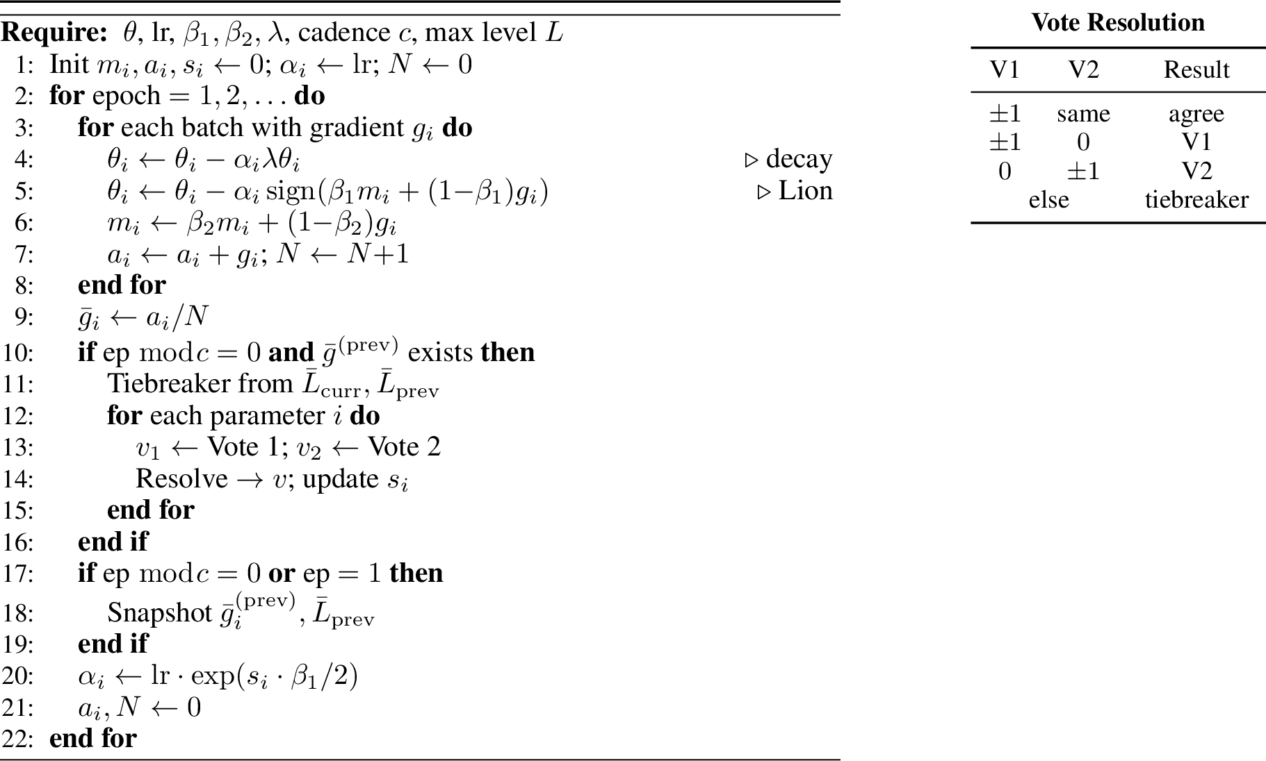
On every training batch, LionVote performs the standard Lion update with \(\alpha_i\) in place of the global learning rate: decoupled weight decay, followed by a sign update \(\operatorname{sign}(\beta_1 m_i + (1 - \beta_1) g_i)\), followed by a \(\beta_2\)-EMA momentum update (Algorithm 1). The raw gradient is accumulated for epoch-level voting.
3.3 Epoch Step and Voting↩︎
At the end of every epoch, LionVote computes the epoch-mean gradient \(\bar{g}_i = a_i / N\) for each parameter, resets the accumulators, and recomputes \(\alpha_i\) from the current \(\mathrm{lr}\) so that per-layer rates track any external scheduler. On voting epochs—epochs where \(\mathrm{epoch} \bmod c = 0\), with \(c\) the voting cadence—the system additionally evaluates two per-layer diagnostics and one global tiebreaker.
3.3.0.1 Vote 1: Gradient Direction Stability.
\[\mathrm{alignment}_i \;=\; \frac{\bar{g}_i^{(\mathrm{curr})} \cdot \bar{g}_i^{(\mathrm{prev})}}{\|\bar{g}_i^{(\mathrm{curr})}\| \, \|\bar{g}_i^{(\mathrm{prev})}\| + \epsilon}.\] The vote is \(+1\) if \(\mathrm{alignment}_i > 0.5\), \(-1\) if \(\mathrm{alignment}_i < 0\), and \(0\) otherwise (\(\epsilon = 10^{-8}\) throughout). The lower threshold follows directly from the definition of cosine (negative iff angle exceeds \(\pi/2\)); the upper threshold corresponds to a two-thirds supermajority of coordinate sign pairs agreeing under coordinate isotropy (Appendix 7.1). Vote 1 uses epoch-mean gradients rather than momentum to avoid self-contamination from the EMA.
3.3.0.2 Vote 2: Momentum Health.
\[r_i \;=\; \frac{\|m_i\|}{\|\bar{g}_i^{(\mathrm{curr})}\| + \epsilon}.\] The vote is \(-1\) if \(r_i > e\) (momentum norm exceeds gradient norm by more than a factor of \(e\)), \(+1\) if \(r_i < 1/e\) (gradient norm exceeds momentum norm by more than a factor of \(e\)), and \(0\) otherwise. Both thresholds derive from the EMA’s intrinsic time constant: \(\beta_2^{\tau} = e^{-1}\) for any \(\beta_2 \in (0,1)\) (Appendix 7.2).
3.3.0.3 Tiebreaker: Validation Loss.
The tiebreaker is a global scalar that fires only when the two local votes sum to zero (both abstain or conflict): \[\delta \;=\; \frac{\bar{L}_{\mathrm{prev}} - \bar{L}_{\mathrm{curr}}}{|\bar{L}_{\mathrm{prev}}| + \epsilon}.\] It returns \(+1\) if \(\delta > 0.01\), \(-1\) if \(\delta < -0.01\), and \(0\) otherwise (\(\epsilon = 10^{-8}\) as in Votes 1 and 2). The \(1\%\) threshold matches the noise floor of cross-entropy loss estimation for typical validation set sizes (Appendix 7.3). Under Lion on ViT-Tiny/CIFAR-100, the tiebreaker condition is satisfied for \({\sim}59\%\) of per-parameter voting decisions (Appendix 8.6), so the tiebreaker is not a tie-breaking edge case but the dominant signal path; Vote 1 or Vote 2 alone determine the outcome for the remaining \({\sim}41\%\).
3.3.0.4 Vote Resolution.
Vote 1 monitors directional stability; Vote 2 monitors the momentum-gradient magnitude ratio. The final vote is resolved per the table in Algorithm 1.
3.4 Compound Level Update↩︎
The compound level \(s_i\) is updated via the asymmetric rule: vote \(= +1\) resets \(s_i\) to \(0\) if negative, else increments (capped at \(+L\)); vote \(= -1\) resets to \(0\) if positive, else decrements (capped at \(-L\)); vote \(= 0\) decays toward zero. A single opposing vote revokes the accumulated level entirely.
3.5 Algorithm↩︎
Computational cost is detailed in Appendix 8.18.
4 Experiments↩︎
We evaluate LionVote against AdamW, SGD with Nesterov momentum, and Lion on four model–dataset configurations. All experiments use 8 random seeds. We report top-1 validation accuracy (mean \(\pm\) std) and epochs to reach intermediate accuracy thresholds.
4.1 Experimental Setup↩︎
4.1.0.1 Models and datasets.
WideResNet-28-10 [5] on CIFAR-10 (\({\sim}36.5\)M parameters, 200 epochs, batch size 128) and WideResNet-40-10 on CIFAR-100 (\({\sim}55.8\)M parameters, 200 epochs, batch size 128). ViT-Tiny [6] (patch size 4, embedding dimension 192, 12 blocks, 3 heads, \({\sim}5.7\)M parameters) on CIFAR-10 and CIFAR-100 (300 epochs, batch size 128). WideResNet uses pre-activation blocks with BatchNorm and dropout 0.3. ViT-Tiny uses learnable positional embeddings, stochastic depth (linearly increasing to 0.1), and a CLS token classification head.
4.1.0.2 Augmentation.
CNN configurations: RandomCrop, HorizontalFlip, and AutoAugment (CIFAR-10 policy) for CIFAR-100. ViT configurations: RandAugment\((2, 9)\), RandomErasing\((p{=}0.25)\), Mixup\((\alpha{=}0.8)\)/CutMix\((\alpha{=}1.0)\) (50/50 per batch), and label smoothing 0.1 with soft cross-entropy.
4.1.0.3 Optimizers.
AdamW (lr\({=}10^{-3}\)), SGD (lr\({=}0.1\), momentum 0.9, Nesterov), Lion (lr\({=}10^{-4}\), \(\beta_1{=}0.9\), \(\beta_2{=}0.99\)), and LionVote (same as Lion, plus voting). Weight decay follows the Lion paper [3]: Lion and LionVote use \(3\)–\(10{\times}\) larger WD than AdamW (e.g.\(5{\times}10^{-1}\) vs.\(5{\times}10^{-2}\) for ViT/CIFAR-10). Full weight decay values per configuration are in Appendix 8. LARS and LAMB are omitted: both are stateless norm-ratio methods designed for large-batch distributed training (§2.2), a different regime from the single-GPU setting studied here.
4.1.0.4 Schedulers.
WRN configurations: cosine annealing. ViT configurations: 5-epoch linear warmup followed by cosine annealing. LionVote is additionally tested without any schedule.
4.1.0.5 Voting hyperparameters.
Cadence \(c \in \{4, 6, 8\}\), max level \(L{=}4\), asymmetric update rule. All voting thresholds are derived (Appendix 7.1–7.3); cadence is selected by ablation within a structurally bounded range (Appendix 7.6).
4.2 Main Results↩︎
| Configuration | SGD | AdamW | Lion | LionVote (c4) | LionVote (c8) |
|---|---|---|---|---|---|
| WRN-28-10 / C10 | 96.08\(\pm\)0.15 | 93.80\(\pm\)0.69 | 93.71\(\pm\)0.40 | 93.14\(\pm\)0.38 | 93.30\(\pm\)0.82 |
| WRN-40-10 / C100 | 82.76\(\pm\)0.37 | 77.45\(\pm\)0.44 | 76.53\(\pm\)0.63 | 76.81\(\pm\)1.26 | 75.81\(\pm\)1.19 |
| ViT-Tiny / C10 | 69.20\(\pm\)1.54 | 91.52\(\pm\)0.21 | 92.40\(\pm\)0.10 | 90.80\(\pm\)0.44 | 91.52\(\pm\)0.18 |
| ViT-Tiny / C100 | 36.97\(\pm\)5.86 | 68.75\(\pm\)0.39 | 68.95\(\pm\)0.41 | 68.90\(\pm\)0.48 | 69.71\(\pm\)0.60 |
SGD with cosine annealing dominates the WRN configurations (Table 1), outperforming the next-best method by \(2.3\) pp on CIFAR-10 and \(5.3\) pp on CIFAR-100, consistent with the established difficulty of beating tuned SGD on uniform CNN architectures [22]. On ViTs, Lion outperforms both SGD and AdamW. LionVote at cadence 8 achieves the best result on ViT-Tiny/CIFAR-100 (\(69.71\%\)) and ties AdamW on ViT-Tiny/CIFAR-10 (\(91.52\%\)). The ViT-Tiny/CIFAR-100 improvement over Lion is statistically significant (Welch’s \(t\)-test, \(p = 0.017\), 8 seeds); cadence is selected by ablation from \(c \in \{4, 6, 8\}\) (§5.3). On ViT-Tiny/CIFAR-10, Lion’s advantage over LionVote at cadence 8 (\(92.40\%\) vs. \(91.52\%\)) is also significant (\(p < 0.001\)). At cadence 8, the differences between Lion and LionVote are not significant on either WRN configuration (\(p > 0.15\)). At cadence 4, LionVote significantly underperforms Lion on WRN-28-10/CIFAR-10 (\(-0.57\) pp, \(p = 0.011\)).
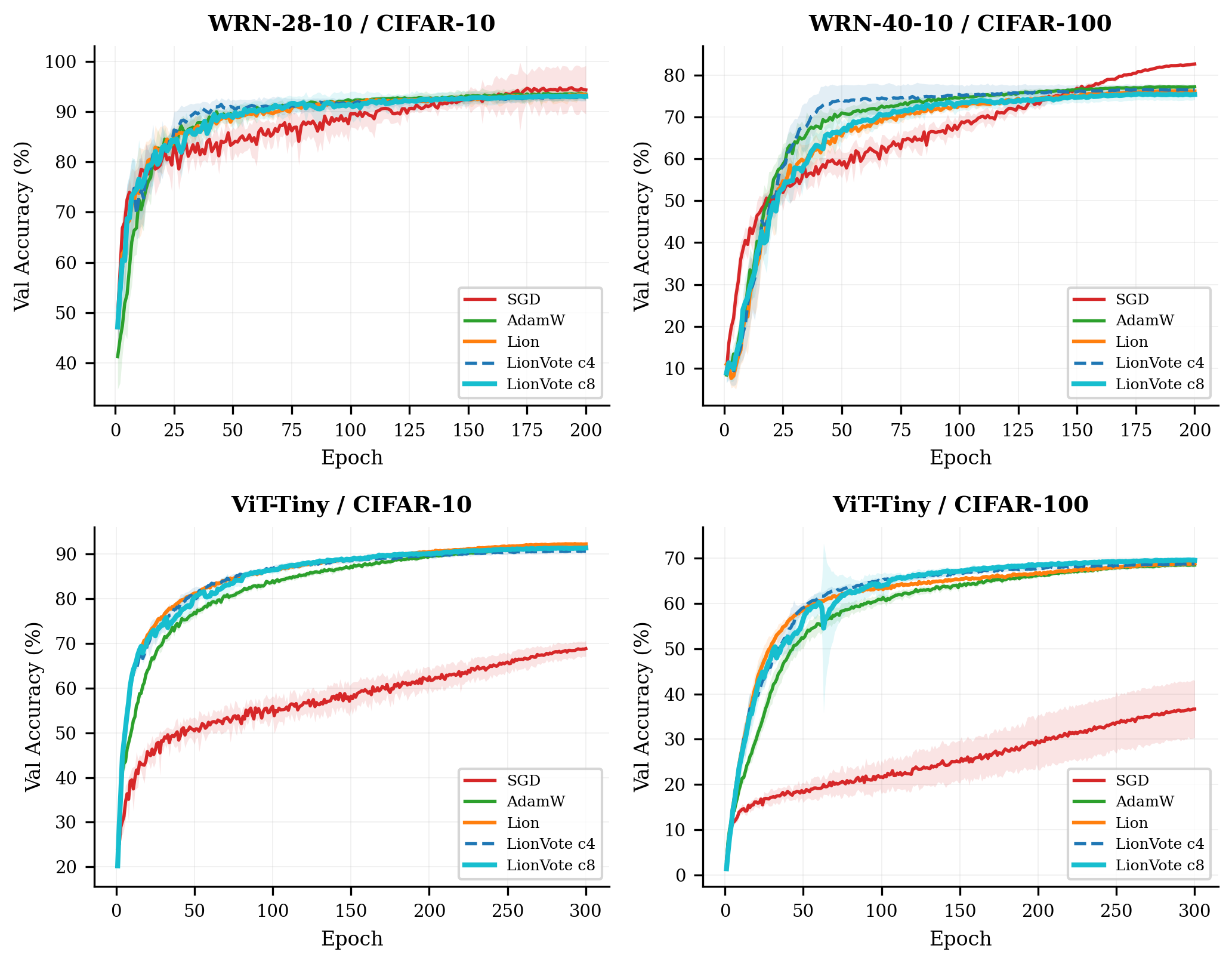
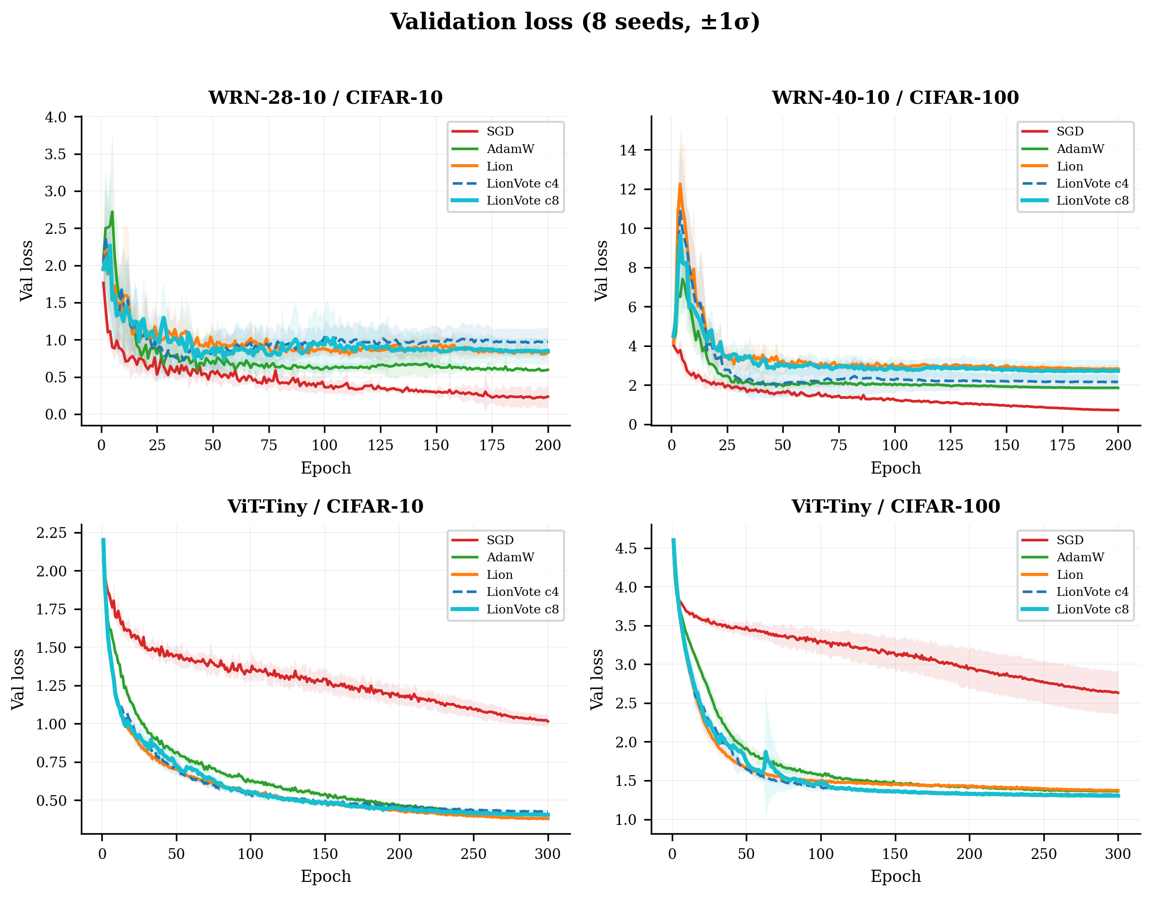
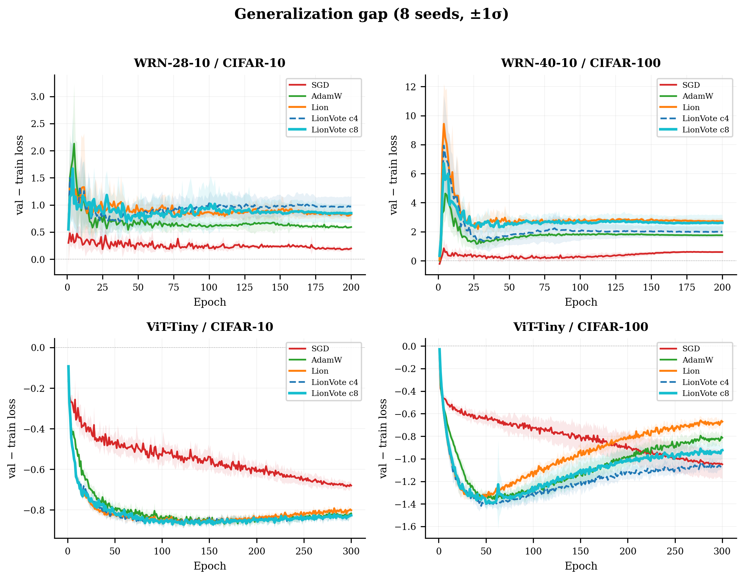
LionVote at cadence 8 reaches the \(68\%\) threshold \({\sim}80\) epochs before Lion on ViT-Tiny/CIFAR-100 (Figure 2; full convergence thresholds in Appendix, Table 8). Validation loss curves and generalisation gap analysis are in Appendix 8.13 and 8.14.
4.3 Ablation Study↩︎
| Variant | Description | WRN/C10 | ViT/C100 |
|---|---|---|---|
| Lion | no voting | 93.71\(\pm\)0.40 | 68.95\(\pm\)0.41 |
| LionVote (c4) | full system | 93.14\(\pm\)0.38 | 68.90\(\pm\)0.48 |
| LionVote (c8) | full, cadence 8 | 93.30\(\pm\)0.82 | 69.71\(\pm\)0.60 |
| v2only | Vote 2 only | 93.46\(\pm\)0.68 | 68.93\(\pm\)0.41 |
| v1only | Vote 1 only | 92.22\(\pm\)0.64 | 68.57\(\pm\)0.49 |
| notie | no tiebreaker | 92.55\(\pm\)0.34 | 68.64\(\pm\)0.52 |
| symmetric | symmetric update | 92.88\(\pm\)0.96 | 70.54\(\pm\)0.94 |
| LionVote+none (c4) | no schedule | 93.02\(\pm\)0.52 | 67.89\(\pm\)0.70 |
| LionVote+none (c8) | no schedule | 93.48\(\pm\)0.39 | 68.89\(\pm\)0.68 |
Vote 2 monitors momentum health and finds it stable. The v2only variant matches Lion on both configurations (\(93.46\%\) WRN/C10, \(68.93\%\) ViT/C100); the momentum-to-gradient ratio rarely exits the \([1/e, e]\) dead zone (Appendix 8.5).
The dominant component is configuration-dependent. On WRN/C10, the v1only variant (which disables both Vote 2 and the tiebreaker) degrades to \(92.22\%\), a \(0.92\) pp gap from the full system (\(93.14\%\)). Of this gap, \(0.59\) pp is attributable to the tiebreaker (Welch \(p = 0.006\)); the remaining \(0.33\) pp attributed to Vote 2 is not significant (\(p = 0.23\)), consistent with its near-zero firing rate. On ViT/C100, the pattern reverses: v1only achieves \(68.57\% \pm 0.49\), below Lion (\(-0.38\) pp, \(p = 0.12\)); notie achieves \(68.64\% \pm 0.52\) (\(-0.31\) pp vs.Lion, \(p = 0.22\)), while the full system at cadence 8 reaches \(69.71\%\) (\(+0.76\) pp, \(p = 0.017\)). The entire gain on ViT/C100 is attributable to the tiebreaker: LionVote c8 exceeds notie by \(+1.07\) pp (\(p = 0.003\)). Vote 1 alone and Vote 1+2 without the tiebreaker both fall below Lion (neither difference significant). LionVote thus combines per-layer gradient diagnostics with a global validation loss signal: Vote 1 provides differentiated per-layer votes (negative \(56\%\) of the time for attention vs.\(30\%\) for normalisation), while the tiebreaker applies the same direction to all undecided layers whenever Vote 1 abstains (approximately \(43\%\) of voting epochs for attention/MLP and \(69\%\) for normalisation, estimated from standard Lion gradient statistics; Appendix 8.16). The per-layer mechanism creates divergent compound level trajectories (Figure 3), but the global tiebreaker signal is necessary to convert this differentiation into an accuracy gain on ViT/C100.
The voting mechanism works with either update rule. On the two configurations tested with symmetric updates, the difference from asymmetric is not significant: \(-0.26\) pp on WRN/C10 (\(p = 0.49\)) and \(+0.83\) pp on ViT/C100 (\(p = 0.060\)). The symmetric variant achieves the highest single-configuration accuracy in the study: \(70.54\% \pm 0.94\) on ViT/C100, significantly above Lion (\(+1.59\) pp, \(p = 0.002\)), though with higher cross-seed variance than the asymmetric default (std \(0.94\) vs.\(0.60\)). The choice of update rule is a design decision, not a derivation (§5.3).
5 Analysis↩︎
5.1 Layer-Type Differentiation↩︎
| Layer type | ep4 | ep64 | ep124 | ep184 | ep244 | ep300 | Mult. | SD\(_{\mathrm{seed}}\) |
|---|---|---|---|---|---|---|---|---|
| all_attn | \(-0.50\) | \(-1.36\) | \(-2.12\) | \(-2.55\) | \(-2.49\) | \(-2.15\) | \(0.38\times\) | \(\pm 0.59\) |
| all_mlp | \(-0.52\) | \(-0.99\) | \(-1.73\) | \(-2.28\) | \(-2.34\) | \(-2.29\) | \(0.36\times\) | \(\pm 0.69\) |
| all_norm | \(-0.57\) | \(-0.80\) | \(-0.86\) | \(-1.06\) | \(-1.31\) | \(-1.54\) | \(0.50\times\) | \(\pm 0.26\) |
| embed+patch | \(-0.41\) | \(-1.47\) | \(-1.88\) | \(-2.09\) | \(-2.16\) | \(-2.03\) | \(0.40\times\) | — |
| head+final_norm | \(-0.25\) | \(-1.06\) | \(-1.06\) | \(-1.38\) | \(-0.94\) | \(-1.56\) | \(0.50\times\) | — |
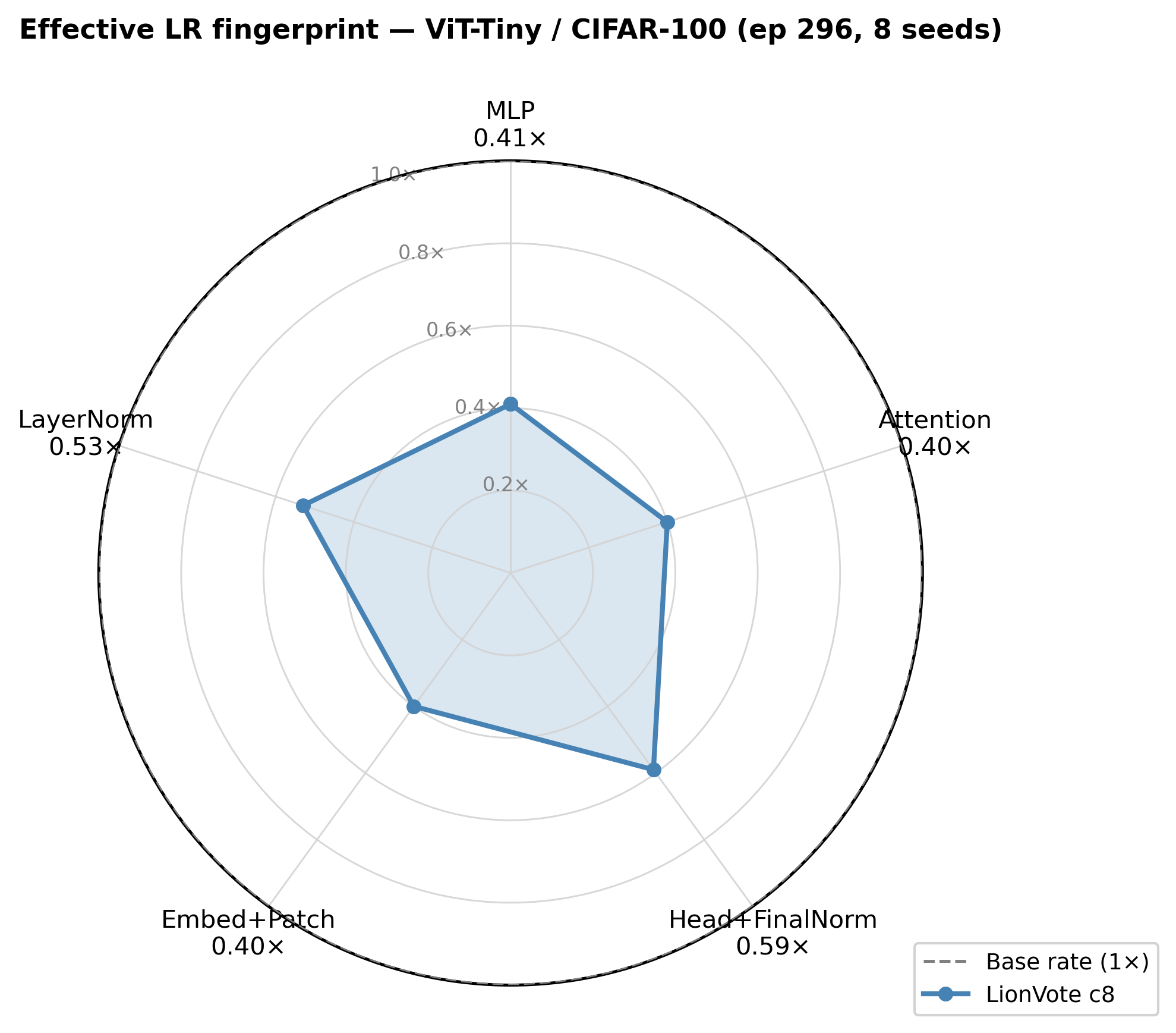
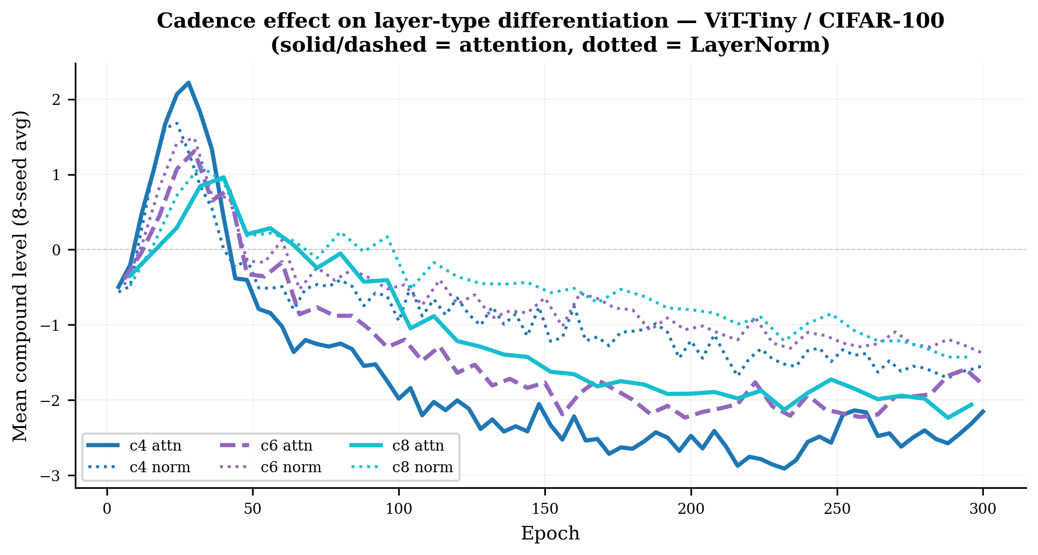
By epoch 300 (Table 3), Lion’s effective scale is \(2.6{\times}\) too high for attention parameters, \(2.8{\times}\) too high for MLP, and \(2.0{\times}\) too high for normalisation. Normalisation layers receive \(32\%\) higher effective scale than attention layers (\(0.50 / 0.38 = 1.32\)); this ratio is consistent at cadence 8 (\(1.33\); Appendix 8.7). Because the compound multiplier \(\alpha_i\) scales both the sign update and decoupled weight decay, the absolute reductions measure joint LR+WD miscalibration, and a global rate reduction cannot reproduce the per-layer differentiation regardless of the LR/WD decomposition.
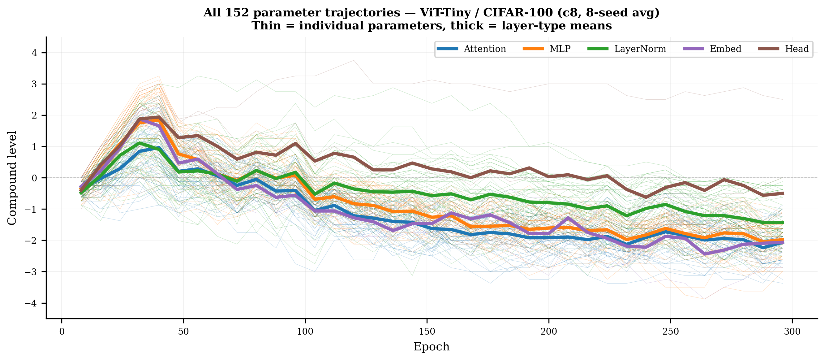
All levels are negative (Figure 3), but the \(32\%\) effective-scale disparity between normalisation and attention layers, consistent across cadence 4 (ratio \(1.32\)) and cadence 8 (ratio \(1.33\); Appendix 8.7), confirms that a uniform rate reduction cannot substitute for per-layer differentiation.
The compound trajectories quantify the disparity that Zhao et al. [1] identify qualitatively on autoregressive language models (§2.2): the layers they flag as needing distinct treatment (normalisation and the classification head) are the same layers that the voting system assigns the highest effective rates.
The differential treatment has a structural basis. LayerNorm parameters are elementwise scalars whose gradient distributions differ qualitatively from the large projection matrices in attention and MLP layers. The voting system detects this through gradient alignment statistics (Vote 1) without requiring architectural knowledge; standard Lion training without voting produces the same layer-type ordering (Appendix 8.16). Cross-optimizer diagnostics confirm the pattern: the attn \(<\) norm ordering holds under both Lion and AdamW, but Lion’s \(\operatorname{sign}(\cdot)\) amplifies the gap (\(1.88{\times}\) larger norm–attn cosine difference; \(0.109\) vs.\(0.058\)). AdamW’s second moment smooths layer-type differences; Lion’s sign operation preserves raw gradient structure, making per-layer adaptation more consequential (Appendix 8.16).
Proposition 3 predicts the observed operating regime: the convergence bound degradation at compound level \(s\) grows as \(\cosh(s \cdot \beta_1/2)\), reaching \(+43\%\) at level \(-2\) where most layer types settle, and \(+106\%\) at level \(-3\) which appears only transiently (Appendix 7.4).
5.1.0.1 What transfers beyond Lion.
Running LionVote’s diagnostics against a paired AdamW trajectory on the same workload (Appendix 8.16) separates the optimizer-agnostic and Lion-specific components of the mechanism. Vote 1’s input signal (cosine of epoch-mean gradients) and firing rates are near-invariant between Lion and AdamW (\(V_1 = -1\) rate \(37.6\%\) vs.\(35.4\%\)); its upper threshold’s derivation uses Lion’s sign structure, but the \(2/3\) supermajority convention is optimizer-agnostic. Vote 2’s thresholds, derived from Lion’s \(\beta_2\)-EMA time constant, misfire under AdamW’s different momentum mechanics (\(V_2 = -1\) fires on \(99.98\%\) of AdamW observations vs.\(2.43\%\) under Lion); these thresholds are Lion-specific and would need re-derivation for transfer. The tiebreaker, compound-level state machine, and cadence/max-level hyperparameters are optimizer-agnostic. A port to another momentum-based optimizer would preserve the voting architecture, recalibrate Vote 2 against that optimizer’s effective momentum time constant, and re-examine the LR exponent. A full breakdown is in Table 18.
5.2 Architecture Dependence↩︎
On WRN-28-10/CIFAR-10, the three residual groups (layer1, layer2, layer3) settle to compound levels of \(-1.68\), \(-1.62\), and \(-1.84\) at epoch 200, a spread of \(0.22\) levels between the most and least reduced groups (Appendix 8.7). On ViT-Tiny, the spread between attention (\(-2.15\)) and normalisation (\(-1.54\)) is \(0.61\) levels, \(2.8{\times}\) larger.
The difference reflects architectural heterogeneity. WRN groups are structurally uniform: each is a sequence of conv+BN blocks with the same connectivity pattern at different spatial resolutions. ViT blocks contain three qualitatively different layer types, each with distinct gradient dynamics. The voting system finds more to differentiate in the ViT.
However, heterogeneity is necessary but not sufficient. At cadence 8, the ViT attn-norm spread is \(0.64\) levels on CIFAR-10 and \(0.63\) levels on CIFAR-100 (nearly identical), yet LionVote significantly helps on CIFAR-100 (\(+0.76\) pp, \(p = 0.012\)) and significantly hurts on CIFAR-10 (\(-0.88\) pp, \(p < 0.001\)), where all cadences degrade performance. What distinguishes CIFAR-100 from CIFAR-10 is not architectural spread but a task-level factor; two tasks do not suffice to identify it. Additional architectures and tasks are needed to map the boundary of per-layer adaptation value.
LionVote without a schedule matches its scheduled variant on WRN/C10 but falls short on ViT/C100 (Appendix 8.17).
5.3 Limitations↩︎
Experiments are limited to CIFAR-10 and CIFAR-100 with WideResNet and ViT-Tiny. The scope is deliberate: every configuration is run with 8 random seeds to eliminate variance-driven conclusions, a level of replication that is incompatible with large-scale experiments under limited compute. Whether the layer-type differentiation observed here (attention/MLP penalised relative to normalisation) holds at larger scale and on different architectures is an open question.
5.3.0.1 Testing hierarchy.
Cadence is selected by ablation from \(c \in \{4, 6, 8\}\), making the LionVote c8 vs.Lion comparison partially post-hoc. Four control experiments on ViT-Tiny/CIFAR-100 (8 seeds each; Appendix 8.15) test the per-layer adaptation claim. Lion at a uniformly lower LR (\(4{\times}10^{-5}\), matching LionVote’s average effective rate) is indistinguishable from standard Lion (\(p = 0.30\)) and significantly below LionVote c8 (\(p = 0.003\), survives Bonferroni correction). Static per-layer-type multipliers (epoch-300 values from Table 3) perform worse than standard Lion (\(p = 0.024\)), confirming that the non-monotonic trajectory cannot be replicated by static scheduling. A weight decay sweep (\(\mathrm{wd} \in \{0.25, 0.5, 0.75\}\)) does not close the gap (\(p \geq 0.075\)). The \(c{=}8\) vs.Lion comparison (\(p = 0.017\)) is marginal after Holm–Bonferroni correction; the primary evidence rests on the control comparison. The study is underpowered below Cohen’s \(d \approx 0.8\).
5.3.0.2 Practitioner guidance.
LionVote at cadence 8 is most likely to help on architectures with qualitatively distinct layer types (ViT-style). On uniform CNNs or tasks where Lion is near its ceiling, it provides no consistent advantage.
5.3.0.3 Additional limitations.
The tiebreaker uses validation loss during training (\({\sim}37\) decisions at cadence 8); future work should confirm on a held-out split. Vote 2 rarely fires at Lion’s recommended rate (§4.3). LionVote exhibits higher cross-seed variance than Lion (e.g.std \(0.82\) vs.\(0.40\) on WRN-28-10/C10). The symmetric variant (\(70.54\%\) on ViT/C100, \(p = 0.002\)) was tested on only 2 of 4 configurations.
6 Conclusion↩︎
LionVote is a per-layer learning rate mechanism for Lion whose voting thresholds are derived from mathematical structure rather than tuned. Three findings are useful beyond the specific method.
First, the threshold derivation methodology (Appendix 7.1–7.6)—Sheppard’s sign-agreement formula, the EMA time constant, and the descent lemma for sign-based updates—provides reusable building blocks for per-layer mechanisms in other optimizers.
Second, Lion’s effective scale is systematically miscalibrated across layer types on ViT-Tiny, with a \(32\%\) disparity between normalisation and attention layers (§5.1). Because the compound multiplier scales both the sign update and decoupled weight decay, this is a joint LR+WD finding. A weight decay sweep (WD\({=}0.25\), WD\({=}0.75\); §5.3) confirms that neither WD adjustment closes the LionVote gap, ruling out simple global WD miscalibration as the explanation and supporting the per-layer adaptation claim. This complements [1] by quantifying the disparity under Lion on vision architectures. Future work on Lion should consider layer-type-aware scaling even without the full voting mechanism. The voting mechanism is not tied to the asymmetric update rule: a symmetric variant achieves \(70.54\%\) on ViT/C100 (\(p = 0.002\) vs. Lion, tested on 2 of 4 configurations), the study’s best single result.
Third, per-layer adaptation provides more value as architectural heterogeneity increases. The compound level spread between layer types is \(2.8{\times}\) larger on ViT-Tiny than on WideResNet, and the accuracy benefit tracks this spread. This suggests that architectures with diverse layer types are the natural setting for per-layer methods.
Open questions include whether the voting mechanism generalises to other sign-based or adaptive optimizers, whether cadence can be adapted during training rather than fixed, and whether training regimes exist—such as higher base learning rates or different \(\beta_2\) values—in which Vote 2 (momentum health) becomes a primary driver of compound level movement.
7 Hyperparameters↩︎
LionVote’s voting thresholds are not tuned. Vote 1’s lower boundary is a geometric identity; its upper boundary connects a classical supermajority convention to a unique cosine threshold via the sign structure of Lion’s update rule. Vote 2’s boundaries follow from the intrinsic timescale of the \(\beta_2\) exponential moving average. The tiebreaker threshold is the noise floor of cross-entropy loss estimation for standard validation set sizes; unlike Votes 1 and 2, it is determined to order of magnitude rather than uniquely. The per-layer LR exponent \(\beta_1/2\) couples to Lion’s momentum-gradient balance through \(\beta_1\) and to the curvature exponent of \(L\)-smooth objectives through the divisor \(2\).
7.1 Vote 1: Gradient Direction Stability (Thresholds 0 and 0.5)↩︎
Vote 1 computes \[c \;=\; \cos(\bar{g}_{\mathrm{curr}},\,\bar{g}_{\mathrm{prev}}),\] the cosine similarity between the current and previous epoch-mean gradient snapshots, and returns \(+1\) if \(c > 0.5\), \(-1\) if \(c < 0\), and \(0\) otherwise. The two thresholds partition \([-1,1]\) into a reversal zone (\(c < 0\)), a dead band (\(c \in [0, 0.5]\)), and a stability zone (\(c > 0.5\)). We justify each boundary in turn, then characterise the dead band.
Lower boundary: \(c = 0\)↩︎
The cosine similarity satisfies \(c < 0\) if and only if the angle between \(\bar{g}_{\mathrm{curr}}\) and \(\bar{g}_{\mathrm{prev}}\) exceeds \(\pi/2\): the epoch-mean gradient has reversed direction across the voting window. This is a complete, parameter-free geometric criterion.
Upper boundary: \(c = 0.5\)↩︎
The lower boundary establishes \(c = 0\) as the onset of positive alignment. The upper threshold determines where alignment is strong enough to warrant a positive vote. Lion applies \(\operatorname{sign}(\cdot)\) coordinate-wise; the operationally relevant quantity for a sign-based update is the fraction of gradient coordinates that maintain their sign between voting epochs. We show that \(c = 0.5\) is the unique threshold corresponding to exactly a two-thirds supermajority of coordinate sign pairs agreeing. This is a consequence of the exact trigonometric identity \(\arccos(1/2) = \pi/3\).
Lemma 1 (Sheppard’s sign-agreement formula). For \((X, Y)\) jointly Gaussian with zero means, equal variances, and correlation \(\rho \in (-1,1)\), \[P\!\bigl(\operatorname{sign}(X) = \operatorname{sign}(Y)\bigr) \;=\; 1 - \frac{\arccos(\rho)}{\pi}.\]
Proof. \[\begin{align} P(XY > 0) &= 2\,P(X > 0,\,Y > 0) = 2\!\left[\frac{1}{4} + \frac{\arcsin(\rho)}{2\pi}\right] = \frac{1}{2} + \frac{\arcsin(\rho)}{\pi} = 1 - \frac{\arccos(\rho)}{\pi}, \end{align}\] using \(\arcsin(\rho) + \arccos(\rho) = \pi/2\). ◻
Theorem 1 (Sign-agreement at the upper threshold). Assume coordinate isotropy: for each coordinate \(i\), the pair \((\bar{g}_{\mathrm{curr},i},\,\bar{g}_{\mathrm{prev},i})\) is drawn from a bivariate zero-mean Gaussian with equal variances and correlation \(c\). At \(c = 0.5\), the probability that a coordinate pair agrees in sign is exactly \(2/3\). Moreover, \(c = 0.5\) is the unique value in \((-1,1)\) for which this probability equals \(2/3\).
Proof. Since \(\arccos(1/2) = \pi/3\) exactly, Lemma 1 gives \(P = 1 - (\pi/3)/\pi = 2/3\). Uniqueness follows from the bijectivity of \(\arccos\) on \([-1,1]\): the equation \(1 - \arccos(\rho)/\pi = 2/3\) has the unique solution \(\rho = 1/2\). ◻
The threshold \(c = 0.5\) is therefore the unique value in \((-1,1)\) at which a two-thirds supermajority of gradient coordinate sign pairs are stable across voting epochs.
Remark 1. The coordinate isotropy assumption treats each coordinate pair as drawn from a common bivariate Gaussian whose correlation equals the global cosine similarity \(c\). Under gross violations of this assumption the sign-agreement probability at \(c = 0.5\) may differ from \(2/3\), and Theorem 1 should be read as an approximation in those cases.
7.1.0.1 Empirical validation.
On ViT-Tiny/CIFAR-100 (seed 2, cadence 8), the per-coordinate sign-agreement fraction was measured at each voting epoch for all parameters whose global cosine similarity falls within a given bin. Table 4 compares the Sheppard prediction (Lemma 1) against the observed fraction.
| Cosine bin | Predicted | Observed | \(n\) |
|---|---|---|---|
| \([0.30, 0.35)\) | \(0.605\) | \(0.615\) | 85 |
| \([0.35, 0.40)\) | \(0.622\) | \(0.634\) | 91 |
| \([0.40, 0.45)\) | \(0.640\) | \(0.657\) | 57 |
| \([0.45, 0.50)\) | \(0.658\) | \(0.684\) | 37 |
| \([0.50, 0.55)\) | \(0.676\) | \(0.684\) | 22 |
| \([0.55, 0.60)\) | \(0.695\) | \(0.727\) | 17 |
| \([0.60, 0.65)\) | \(0.715\) | \(0.766\) | 9 |
| \([0.65, 0.70)\) | \(0.736\) | \(0.781\) | 7 |
At \(c \in [0.45, 0.55]\) (\(n = 59\) measurements), the mean observed sign agreement is \(0.684\), within \(2.6\%\) of the predicted \(2/3\). The prediction tracks the data across the full range \(c \in [0.3, 0.7]\), with a consistent positive bias of \(1\)–\(7\%\) (increasing with cosine; upper bins have \(n < 10\)): real ViT-Tiny gradients exhibit slightly more sign agreement than coordinate isotropy predicts. The bias makes the \(0.5\) threshold conservative—the true two-thirds boundary lies slightly below \(0.5\). This is a single-seed measurement; the direction of the bias is consistent across all eight cosine bins. The \(2/3\) supermajority convention is itself a design choice; Appendix 8.4 sweeps the resulting upper threshold across \([0.3, 0.7]\) on recorded Lion diagnostics and shows the vote composition does not sit near a phase transition in this range.
Dead band↩︎
The two boundaries together define the dead band \(c \in [0, 0.5]\). Within it, the gradient direction has not reversed, but under the coordinate isotropy model strictly fewer than two-thirds of coordinate sign pairs are stable. Vote 1 abstains, treating this as an ambiguous regime where neither direction is warranted.
7.2 Vote 2: Momentum Health (Thresholds \(1/e\) and \(e\))↩︎
Vote 2 computes \[r \;=\; \frac{\|m\|}{\|\bar{g}_{\mathrm{curr}}\| + \epsilon},\] the ratio of the momentum EMA norm to the epoch-mean gradient norm, and returns \(-1\) if \(r > e\), \(+1\) if \(r < 1/e\), and \(0\) otherwise. Both thresholds derive from the EMA’s intrinsic timescale as a single symmetric pair.
Lemma 2 (EMA time-constant identity). The EMA \(m_t = \beta_2 m_{t-1} + (1-\beta_2)g_t\) has time constant \(\tau = -1/\ln\beta_2\). For any \(\beta_2 \in (0,1)\), \[\beta_2^{\,\tau} \;=\; e^{-1}.\]
Proof. Consider the unit-step response: if \(g_t\) switches from \(0\) to \(1\) at \(t=0\), unrolling the recurrence gives \[m_t \;=\; 1 - \beta_2^{\,t}.\] In standard signal-processing usage, the time constant \(\tau\) of such a first-order system is the time at which the step response reaches \(1 - 1/e \approx 63.2\,\%\) of its final value. Setting \(m_\tau = 1 - 1/e\): \[1 - \beta_2^{\,\tau} \;=\; 1 - \frac{1}{e} \qquad\Longrightarrow\qquad \beta_2^{\,\tau} \;=\; e^{-1}.\] Taking logarithms of both sides, \[\tau\ln\beta_2 \;=\; -1 \qquad\Longrightarrow\qquad \tau \;=\; -\frac{1}{\ln\beta_2}.\] No free parameter enters: the identity \(\beta_2^{\,\tau} = e^{-1}\) holds for every \(\beta_2 \in (0,1)\). ◻
Under stationarity, the EMA converges in mean to the gradient mean (\(\mathbb{E}[m_t] = \mathbb{E}[g_t]\)), so \(r\) concentrates near \(1\). Deviations signal non-stationarity.
Proposition 2 (Ratio dynamics after a gradient magnitude change). Suppose the EMA has converged to \(m_0 = A\hat{u}\) and the gradient magnitude changes instantaneously from \(A\) to \(B\) with direction preserved (\(\hat{u}\) denotes the common unit direction). Then for \(t \geq 0\), \[r(t) \;=\; \frac{\|m_t\|}{B} \;=\; 1 + \beta_2^t\!\left(\frac{A}{B}-1\right).\] In particular, \(r(0) = A/B\).
Proof. Direction is preserved, so \(\|m_t\| = \beta_2^t A + (1-\beta_2^t)B\). Dividing by \(B\) gives the result. ◻
Corollary 1 (The \((1/e,\,e)\) threshold pair). The pair \((1/e,\,e)\) is the unique symmetric pair \((a,\,1/a)\) with \(a \in (0,1)\) satisfying \(a = \beta_2^{\tau}\). The interval \([1/e,\,e]\) has log half-width exactly 1, the natural unit of the EMA’s exponential decay \(\beta_2^t = e^{-t/\tau}\), and is the only log-symmetric interval \([e^{-\kappa},\,e^{\kappa}]\) centred at \(1\) whose boundary coincides with \(\beta_2^{\tau}\).
Proof. By Lemma 2, \(\beta_2^{\tau} = 1/e\) for all \(\beta_2 \in (0,1)\). Setting \(a = \beta_2^{\tau}\) gives \(a = 1/e\) and \(1/a = e\) uniquely. The log half-width of the interval is \(\ln e = 1\). Any alternative pair \((e^{-\kappa},\,e^{\kappa})\) with \(\kappa \neq 1\) would satisfy \(e^{-\kappa} \neq \beta_2^{\tau}\) and would require an independent choice of \(\kappa\). ◻
From Proposition 2, \(r(0) = A/B = e\) corresponds to an instantaneous gradient magnitude drop by a factor of exactly \(e\). Corollary 1 identifies \(e\) as the EMA’s fundamental unit of magnitude change, so \(r = e\) marks a one-time-constant excess of the EMA over the current gradient: the upper threshold fires when the EMA retains more than one time-constant’s worth of surplus signal. Symmetrically, \(r = 1/e\) marks a one-time-constant deficit, where the gradient has surged by more than one \(e\)-fold relative to the EMA. The dead zone \(r \in [1/e,\,e]\) spans exactly two units in log scale.
Remark 2. Proposition 2 characterises \(r\) at \(t = 0\), immediately after an instantaneous magnitude change. In practice, \(r\) is measured at epoch end: after \(N\) training steps the EMA has already begun adapting, and the observed ratio is closer to \(1\) than \(r(0) = A/B\). Vote 2 therefore fires only when the gradient magnitude has been persistently shifted over many steps, not after a transient change. The thresholds \(1/e\) and \(e\) are principled anchors calibrated to the EMA’s natural unit, not exact characterisations of a specific trajectory.
7.3 Tiebreaker: Validation Loss (Threshold \(\pm 1\%\))↩︎
Unlike Votes 1 and 2, whose thresholds derive from mathematical identities independent of any experimental parameter, the tiebreaker threshold depends on the validation set size \(n\). We show that for \(n \approx 10^4\), the \(\pm 1\%\) relative threshold matches the intrinsic noise floor of cross-entropy loss estimation.
The tiebreaker computes the relative loss improvement \[\delta \;=\; \frac{\bar{L}_{\mathrm{prev}} - \bar{L}_{\mathrm{curr}}}{|\bar{L}_{\mathrm{prev}}| + \epsilon},\] where \(\bar{L} = \frac{1}{n}\sum_{i=1}^{n}\ell_i\) is the mean validation loss with \(\ell_i = -\log p_{\mathrm{correct},i}\), and returns \(+1\) if \(\delta > 0.01\), \(-1\) if \(\delta < -0.01\), and \(0\) otherwise.
By the central limit theorem, the standard error of \(\bar{L}\) is \(\sigma_\ell/\sqrt{n}\). Dividing by \(\bar{L}\) gives the relative standard error \[\mathrm{RSE} \;=\; \frac{\sigma_\ell}{\bar{L}\,\sqrt{n}} \;=\; \frac{\mathrm{CV}_\ell}{\sqrt{n}},\] where \(\mathrm{CV}_\ell = \sigma_\ell/\bar{L}\) is the coefficient of variation of the per-sample loss.
The threshold therefore reduces to a question about \(\mathrm{CV}_\ell\). For cross-entropy loss on a trained but imperfect classifier, the loss \(\ell_i = -\log p_{\mathrm{correct},i}\) is supported on \([0,\infty)\) and right-skewed: most predictions have high confidence and low loss, while a minority of hard examples have low confidence and high loss. Both \(\bar{L}\) and \(\sigma_\ell\) are dominated by this same right tail, so their ratio \(\mathrm{CV}_\ell\) stays \(\Theta(1)\) across models, datasets, and training stages.
At \(n \approx 10^4\) this gives \(\mathrm{RSE} \approx \mathrm{CV}_\ell / \sqrt{n} = \Theta(1\%)\). The \(1\%\) threshold is therefore the order of magnitude of the noise floor at this validation set size. It is not uniquely determined: nearby values would be comparably justified. It serves as a round threshold that separates genuine loss movement from estimation noise.
Remark 3. The tiebreaker compares validation losses computed on the same fixed sample set at consecutive voting epochs. This paired structure has strictly smaller standard error than the unpaired RSE derived above, because the per-sample loss differences \(d_i = \ell_i^{(t)} - \ell_i^{(t-c)}\) have lower variance than the losses themselves when the model changes only gradually. The \(1\%\) threshold is therefore conservative: it acts only when the signal exceeds the noise floor of a single unpaired measurement.
Remark 4. For validation sets of substantially different size, the noise floor shifts as \(\mathrm{CV}_\ell/\sqrt{n}\). At larger \(n\) the noise floor drops below \(1\%\) and the fixed threshold becomes more conservative, potentially missing genuine but modest loss changes. At smaller \(n\) the noise floor exceeds \(1\%\) and the fixed threshold becomes too aggressive, potentially acting on sampling noise. A size-adaptive threshold \(\mathrm{CV}_\ell/\sqrt{n}\) is a natural extension. We use the fixed value \(0.01\) for simplicity.
7.4 LR Exponent: \(\beta_1/2\)↩︎
The per-layer learning rate formula \[\alpha_i \;=\; \mathrm{lr} \cdot \exp\!\bigl(s_i \cdot \beta_1 / 2\bigr)\] involves two choices: \(\beta_1\) as the numerator and \(2\) as the divisor. The numerator follows from Lion’s momentum-gradient structure. The divisor coincides with the curvature exponent universal to \(L\)-smooth objectives.
Numerator: \(\beta_1\)↩︎
The boundary behaviours of \(\beta_1\) pin down the numerator. At \(\beta_1 = 0\), \(\exp(s_i \cdot 0/2) = 1\) for all \(s_i\), so \(\alpha_i = \mathrm{lr}\) uniformly and per-layer modulation vanishes. The modulation range \(\alpha_{+L}/\alpha_{-L} = \exp(L \cdot \beta_1)\) is strictly increasing in \(\beta_1\) (since \(L > 0\)), and reaches its maximum \(\exp(L)\) at \(\beta_1 = 1\).
These boundaries reflect the optimizer’s structure. When \(\beta_1 = 0\), Lion’s update rule reduces to \(\operatorname{sign}(g)\): the current gradient alone, with no dependence on momentum history [3]. Every layer receives the same quality of learning signal regardless of convergence state, so per-layer modulation is unnecessary and the formula correctly produces none. As \(\beta_1 \to 1\), the update approaches \(\operatorname{sign}(m)\): pure momentum. Layers that have been learning in a stable direction accumulate useful momentum, while layers in noisy or transitioning regimes accumulate stale or contradictory momentum.
Making the exponent proportional to \(\beta_1\) is the simplest form that (a) vanishes when momentum is absent, (b) grows monotonically with the momentum fraction, and (c) introduces no free parameter beyond those already present in the optimizer.
Remark 5. This is a design argument, not a uniqueness theorem. The boundary behaviours constrain the numerator to be a function that equals zero at \(\beta_1 = 0\), is positive for \(\beta_1 > 0\), and is increasing. The simplest such function is \(\beta_1\) itself. Other increasing functions vanishing at zero, such as \(\beta_1^2\) or \(\sqrt{\beta_1}\), satisfy the same boundary conditions but introduce curvature with no structural motivation.
Divisor: \(2\)↩︎
The divisor determines the per-level granularity of learning rate adaptation. We derive a quantitative criterion from the convergence bound of sign-based methods on \(L\)-smooth objectives.
Under coordinate-wise \(L\)-smoothness, one step of a sign-based update \(x_{k+1} = x_k - \alpha\,\operatorname{sign}(v_k)\) satisfies \[f(x_{k+1}) \;\le\; f(x_k) - \alpha\,\langle \nabla\! f(x_k),\,\operatorname{sign}(v_k) \rangle + \frac{\alpha^2}{2}\,\|\tilde{L}\|_1,\] where \(\|\tilde{L}\|_1 = \sum_i L_i\). This is a consequence of the coordinate-wise smoothness framework of [11] (Theorem 1 and Lemma E.1). The key simplification relative to standard gradient descent is that \(|\operatorname{sign}(\cdot)|^2 = 1\) renders the curvature penalty \((\alpha^2/2)\|\tilde{L}\|_1\) independent of the gradient magnitude.
Telescoping over \(K\) iterations and dividing by \(\alpha K\) yields the convergence bound \[B(\alpha) \;=\; \frac{A}{\alpha} + C\alpha, \qquad A = \frac{\Delta f}{K},\quad C = \frac{\|\tilde{L}\|_1}{2},\] where the first term captures progress (decreasing in \(\alpha\)) and the second captures curvature cost (increasing in \(\alpha\)).
Proposition 3 (Log-LR perturbation cost). The optimal learning rate is \(\alpha^* = \sqrt{A/C}\). At a perturbed rate \(\alpha^* e^\varepsilon\): \[\frac{B(\alpha^*\, e^\varepsilon)}{B(\alpha^*)} \;=\; \cosh(\varepsilon).\] The relative degradation depends only on the log-LR perturbation \(\varepsilon\), not on \(\Delta f\), \(\|\tilde{L}\|_1\), the dimension, or the number of steps.
Proof. At the optimum, \(A / \alpha^* = C\alpha^*\), so \(B(\alpha^*) = 2\sqrt{AC}\). Then \[\begin{align} B(\alpha^* e^\varepsilon) &= \frac{A}{\alpha^* e^\varepsilon} + C\,\alpha^* e^\varepsilon = \sqrt{AC}\,(e^{-\varepsilon} + e^{\varepsilon}) = 2\sqrt{AC}\,\cosh(\varepsilon). \end{align}\] Dividing by \(B(\alpha^*) = 2\sqrt{AC}\) gives \(\cosh(\varepsilon)\). ◻
Each compound level shifts the log-LR by \(\varepsilon = \beta_1/d\), where \(d\) is the divisor. The per-level convergence cost is \(\cosh(\beta_1/d)\), and the worst case at \(\pm L\) levels is \(\cosh(L \cdot \beta_1/d)\). For \(\beta_1 = 0.9\) and \(L = 4\):
| Divisor \(d\) | Per-level \(\varepsilon\) | \(\cosh(\varepsilon)\) | Worst case \(\cosh(4\varepsilon)\) |
|---|---|---|---|
| 1 | 0.90 | 1.433 (+43%) | 18.31 |
| 2 | 0.45 | 1.103 (+10%) | 3.107 |
| 3 | 0.30 | 1.045 (+4.5%) | 1.811 |
At \(d = 1\), the worst-case degradation of \(18\times\) renders the outer levels unusable: a layer at level \(+4\) pays an order-of-magnitude convergence penalty, defeating the purpose of a graded system. At \(d = 3\), the per-level LR factor \(\exp(0.30) \approx 1.35\times\) provides insufficient differentiation per vote, making the voting system sluggish.
At \(d = 2\), each compound level incurs \({\sim}10\%\) convergence bound degradation, and the full \(\pm 4\) range spans from \({\sim}0.17\times\) to \({\sim}6\times\) the base rate. This permits meaningful per-layer adaptation without excessive worst-case cost.
Remark 6. The \(\cosh\) result (Proposition 3) applies per-layer: each layer’s parameters satisfy an independent descent lemma with their own smoothness constants. A layer at compound level \(s\) incurs degradation \(\cosh(s \cdot \beta_1/2)\) relative to the base rate. The per-layer nature of LionVote means these costs do not compound across layers.
Consistency check: edge of stability↩︎
At the edge of stability [23], training dynamics self-organise so that the loss landscape sharpness hovers near the optimizer’s stability threshold. When the learning rate increases, the threshold drops: the loss landscape must flatten for training to remain stable. A one-level LR increase of \(\exp(\beta_1/2) \approx 1.57\times\) is a moderate perturbation; the network has multiple epochs before the next vote to re-equilibrate. Using \(\beta_1\) directly as the exponent (\(d = 1\)) gives \(\exp(0.9) \approx 2.46\times\) per level, a substantially larger perturbation that demands more aggressive landscape rearrangement within the same time window.
Remark 7. The edge of stability was established empirically for full-batch gradient descent, where the spectral norm of the Hessian converges to approximately \(2/\eta\) [23]. For sign-based methods with momentum, the stability mechanism operates through a different sharpness measure and the specific threshold differs. The qualitative principle that increasing the learning rate forces the loss landscape to flatten is general across optimizers and is the basis of this consistency check.
Remark 8. No published result proves \(\beta_1/2\) is uniquely optimal. Any divisor in \([1.5, 3]\) would be defensible. The value \(2\) is the simplest integer in this range and balances per-level cost against modulation range (Table 5).
7.5 Maximum Compound Level↩︎
The compound level is bounded by \(\pm L\), where \(L = \texttt{max\_level}\). The choice of \(L\) involves a trade-off between expressivity (the range of per-layer learning rates) and worst-case convergence cost.
At compound level \(s\) with divisor \(d = 2\), the learning rate multiplier is \(\exp(s \cdot \beta_1/2)\) and the convergence bound degradation is \(\cosh(s \cdot \beta_1/2)\) (Proposition 3). For \(\beta_1 = 0.9\):
| \(L\) | LR range \(\exp(L \cdot \beta_1)\) | Max multiplier \(\exp(L \cdot \beta_1/2)\) | Worst case \(\cosh(L \cdot \beta_1/2)\) |
|---|---|---|---|
| 2 | \({\times}6.0\) | \({\times}2.46\) | 1.433 (+43%) |
| 3 | \({\times}14.9\) | \({\times}3.86\) | 2.058 (\({\times}2.1\)) |
| 4 | \({\times}36.6\) | \({\times}6.05\) | 3.107 (\({\times}3.1\)) |
| 5 | \({\times}90.0\) | \({\times}9.49\) | 4.797 (\({\times}4.8\)) |
| 6 | \({\times}221\) | \({\times}14.9\) | 7.473 (\({\times}7.5\)) |
Two constraints bound \(L\) from above and below.
Lower bound (expressivity). Compound levels are earned through consecutive same-sign votes. At \(L = 2\), the maximum multiplier is \({\times}2.46\), comparable to a single step of a typical schedule drop, and the total LR range is \({\times}6.0\). A system with this range has limited ability to differentiate layers with substantially different convergence needs. At \(L = 3\), the range grows to \({\times}14.9\) and the maximum multiplier to \({\times}3.86\): enough to express meaningful differentiation, but still less than one and a half orders of magnitude.
Upper bound (worst-case cost). The worst-case convergence bound degradation \(\cosh(L \cdot \beta_1/2)\) grows with \(L\). In the table above, the growth accelerates: from \(L = 2\) to \(L = 3\) the worst case increases by \(44\%\) (\(1.43 \to 2.06\)); from \(L = 3\) to \(L = 4\) by \(51\%\) (\(2.06 \to 3.11\)); from \(L = 4\) to \(L = 5\) by \(54\%\) (\(3.11 \to 4.80\)). This reflects the transition of \(\cosh\) from its quadratic regime (\(\cosh(x) \approx 1 + x^2/2\)) to its exponential regime (\(\cosh(x) \approx e^x/2\)). At \(L = 4\), the argument to \(\cosh\) is \(1.8\) and the quadratic approximation \(1 + 1.8^2/2 = 2.62\) underestimates the true value \(3.107\) by \(16\%\). At \(L = 5\), the argument is \(2.25\) and the quadratic approximation gives \(3.53\) versus the true \(4.797\), a \(26\%\) underestimate. The quadratic regime, where \(\cosh\) grows gently, is ending.
\(L = 4\) is the operating point where the LR range first exceeds one and a half orders of magnitude (\({\times}36.6\)) while the worst-case degradation remains below \({\times}3.2\), moderate enough that a layer at the boundary is not catastrophically penalised.
Remark 9. \(L = 3\) (\(\cosh(1.35) \approx 2.06\), range \({\times}14.9\)) is also defensible. \(L = 4\) is preferred because it provides \(2.5{\times}\) the LR range at only \(51\%\) additional worst-case cost, and because finer granularity allows the system to make smaller distinctions between layers at different stages of convergence.
7.6 Voting Cadence↩︎
The voting cadence \(c\) is the number of epochs between consecutive voting events. Unlike the preceding hyperparameters, cadence cannot be derived from a single mathematical identity: it depends on the interaction between the voting system, the compound level update rule, and the training dynamics. We characterise three structural constraints that bound the useful range of \(c\).
Lower bound: EMA convergence↩︎
Vote 2 uses the momentum EMA \(m_t = \beta_2 m_{t-1} + (1 - \beta_2) g_t\). After a learning rate change alters the gradient distribution, the EMA requires \(\tau = -1/\!\ln\beta_2\) steps to track the new mean (Lemma 2). Until the EMA has converged, the momentum-to-gradient ratio \(r\) (Vote 2’s input) reflects the old regime rather than the new one. The voting window must be long enough that the EMA statistics used for voting have equilibrated after any level change from the previous vote.
Lower bound: recovery time↩︎
Under the asymmetric update rule, an opposing vote resets the compound level to zero. After a reset, the system requires up to \(L\) consecutive same-sign votes, i.e.\(L \cdot c\) epochs, to return to the boundary. If \(c\) is too small, the system votes before the gradient statistics have had time to reflect the learning rate change caused by the previous vote. The votes then respond to stale information, producing oscillatory level dynamics.
Upper bound: adaptivity↩︎
The system has at most \(\lfloor E/c \rfloor\) voting opportunities over \(E\) training epochs, minus one for the cold-start reference. The number of voting opportunities must comfortably exceed \(2L\) to allow both upward and downward traversal of the full \([-L, +L]\) range over the course of training. At \(c = 16\) over \(E = 200\) epochs, only \(12\) votes occur; with \(L = 4\), reaching the boundary and returning to zero would consume \(8\) of them, leaving little room for adaptation to changing training dynamics.
Selection within the range↩︎
The constraints above place the useful range at roughly \(c \in [4, 10]\) for typical training lengths (\(E \geq 200\) epochs in this work). Within this range, smaller cadence gives more frequent adaptation at the cost of noisier votes and less recovery time. Larger cadence gives cleaner votes at the cost of fewer total voting opportunities.
Remark 10. Cadence is the one hyperparameter in LionVote that is selected by ablation rather than derived from a mathematical identity. It is bounded from below by EMA convergence time and recovery dynamics, and from above by the need for sufficient voting opportunities. Within the feasible range, the choice is empirical: \(c = 4\) is a conservative default and \(c = 8\) is preferred when total training epochs permit.
7.7 Configuring LionVote↩︎
This subsection consolidates the tunable and non-tunable knobs, their defaults, and guidance for non-default choices.
| Knob | Default | Derivation | Practitioner action |
|---|---|---|---|
| Lion LR | \(10^{-4}\) | – | Use Lion’s recommended rate for the workload. |
| Lion \(\beta_1\) | \(0.9\) | – | Use Lion default (momentum interp). |
| Lion \(\beta_2\) | \(0.99\) | – | Use Lion default (EMA buffer). |
| Weight decay | \(0.5\) | – | Use Lion default for ViT workloads. |
| Cadence \(c\) | \(8\) | App. [sec:app:cadence] | If training \(< 200\) epochs, use \(c = 4\). |
| Max level \(L\) | \(4\) | App. [sec:app:maxlevel] | Saturation rate at \(L = 4\) is \(11.7\%\) (Table [tbl:tab:compound95distribution]); lowering to \(L = 3\) truncates \({\sim}12\%\) of decisions. |
| Vote 1 lower | \(0\) | App. [sec:app:vote1] | Do not change. |
| Vote 1 upper | \(0.5\) | App. [sec:app:vote1] | Do not change; see Table [tbl:tab:v195threshold95sensitivity] for perturbation impact on vote composition. |
| Vote 2 factor | \(e\) | App. [sec:app:vote2] | Do not change; Vote 2 is near-dormant at this value and that is by design. |
| Tiebreaker | \(0.01\) | App. [sec:app:tiebreaker] | Rescale as \(\mathrm{CV}_\ell/\sqrt{n}\) for validation set sizes far from the default. |
| LR exponent divisor | \(2\) | App. [sec:app:exponent] | Do not change; defensible on worst-case (Table [tbl:tab:divisor95comparison]) and realised-mean (Table [tbl:tab:divisor95empirical]) grounds. |
| Asymmetric update rule | enabled | §[sec:sec:experiments:ablation] | Consider the symmetric variant for ViT-style architectures. |
7.7.0.1 Per-iteration and memory cost.
See Appendix 8.18: one additional in-place accumulation per parameter per batch, \(2\) tensors plus \(2\) scalars of extra state per parameter (\(3{\times}\) Lion’s optimizer-state memory), and \(152\) dot products and norms once every \(c\) epochs for ViT-Tiny. For billion-parameter models the \(3{\times}\) state increase should be weighed against Lion’s optimizer-state footprint (\({\sim}2{\times}\) the model parameters).
7.7.0.2 When to expect benefit.
LionVote at cadence \(8\) is most likely to help on architectures with qualitatively distinct layer types (ViT-style). On uniform CNNs or tasks where Lion is near its ceiling, it provides no consistent advantage; see practitioner guidance in §5.3. Per-layer adaptation value increases with architectural heterogeneity (§5.2).
7.7.0.3 Diagnostics-only deployment.
Running LionVote with all votes disabled (and compound levels decaying to zero) is equivalent to plain Lion. This makes diagnostics collection non-invasive: one can deploy LionVote with the voting thresholds set to \(\pm\infty\) (or using a flag) purely to collect the per-layer gradient-alignment and momentum-ratio statistics, then decide whether to enable voting.
8 Experimental Details↩︎
8.1 Weight Decay by Configuration↩︎
Per-config, per-optimizer weight decay values. Lion and LionVote use identical weight decay; all ablation variants inherit LionVote’s values.
| Configuration | AdamW | SGD | Lion / LionVote |
|---|---|---|---|
| WRN-28-10 / CIFAR-10 | \(5 \times 10^{-4}\) | \(5 \times 10^{-4}\) | \(5 \times 10^{-3}\) |
| WRN-40-10 / CIFAR-100 | \(5 \times 10^{-4}\) | \(5 \times 10^{-4}\) | \(5 \times 10^{-3}\) |
| ViT-Tiny / CIFAR-10 | \(5 \times 10^{-2}\) | \(5 \times 10^{-4}\) | \(5 \times 10^{-1}\) |
| ViT-Tiny / CIFAR-100 | \(5 \times 10^{-2}\) | \(5 \times 10^{-4}\) | \(5 \times 10^{-1}\) |
Lion’s weight decay values follow the recommendation of Chen et al. [3] (Section 5): \(3\)–\(10{\times}\) larger WD than AdamW, compensating for Lion’s \(3\)–\(10{\times}\) smaller learning rate. AdamW uses PyTorch’s built-in decoupled weight decay; SGD uses L2 regularisation; Lion and LionVote apply decoupled weight decay manually in the update step.
8.1.0.1 Augmentation note.
CNN configurations on CIFAR-100 use the CIFAR-10 AutoAugment policy. PyTorch’s AutoAugmentPolicy.CIFAR10 is the only CIFAR policy provided in torchvision; no separate CIFAR-100 policy exists. Using the CIFAR-10 policy for both
datasets is standard practice in the CIFAR benchmark literature.
8.2 Full Convergence Threshold Tables↩︎
Table 8 provides selected convergence thresholds for all configurations.
| Configuration | Threshold | SGD | AdamW | Lion | LionVote (c4) | LionVote (c8) |
|---|---|---|---|---|---|---|
| WRN-28-10 / C10 | \(\to\)91% | 110 | 56 | 61 | 41 | 71 |
| \(\to\)92% | 123 | 76 | 82 | 76 | — | |
| \(\to\)95% | 158 | — | — | — | — | |
| WRN-40-10 / C100 | \(\to\)76% | 143 | 119 | — | — | — |
| \(\to\)80% | 169 | — | — | — | — | |
| ViT-Tiny / C10 | \(\to\)89% | — | 180 | 145 | 155 | 136 |
| \(\to\)90% | — | 209 | 173 | 208 | 173 | |
| ViT-Tiny / C100 | \(\to\)67% | — | 214 | 199 | 146 | 133 |
| \(\to\)68% | — | 250 | 239 | 193 | 160 |
Expanded per-configuration convergence tables follow (mean over 8 seeds; “—” = fewer than 8 seeds reached the threshold).
8.2.0.1 WRN-28-10 / CIFAR-10.
| Setup | \(\to\)88% | \(\to\)89% | \(\to\)90% | \(\to\)91% | \(\to\)92% | \(\to\)93% |
|---|---|---|---|---|---|---|
| SGD+cos | 64 | 84 | 95 | 110 | 123 | 136 |
| AdamW+cos | 30 | 38 | 45 | 56 | 76 | — |
| Lion+cos | 33 | 36 | 49 | 61 | 82 | — |
| LionVote+cos | 27 | 31 | 34 | 41 | 76 | — |
| LionVote+cos (c8) | 33 | 40 | 45 | 71 | — | — |
| LionVote+cos (c6) | 31 | 34 | 40 | 53 | 92 | — |
8.2.0.2 WRN-40-10 / CIFAR-100.
| Setup | \(\to\)72% | \(\to\)73% | \(\to\)74% | \(\to\)75% | \(\to\)76% | \(\to\)77% |
|---|---|---|---|---|---|---|
| SGD+cos | 114 | 123 | 128 | 137 | 143 | 150 |
| AdamW+cos | 58 | 66 | 79 | 98 | 119 | — |
| Lion+cos | 81 | 90 | 109 | 136 | — | — |
| LionVote+cos | 51 | 61 | 70 | — | — | — |
| LionVote+cos (c6) | 56 | 66 | 77 | 93 | — | — |
| LionVote+cos (c8) | 73 | 80 | 101 | — | — | — |
8.2.0.3 ViT-Tiny / CIFAR-10.
| Setup | \(\to\)87% | \(\to\)88% | \(\to\)89% | \(\to\)90% | \(\to\)91% | \(\to\)92% |
|---|---|---|---|---|---|---|
| Lion+cos+warm | 105 | 121 | 145 | 173 | 211 | 257 |
| AdamW+cos+warm | 137 | 161 | 180 | 209 | 249 | — |
| LionVote+cos+warm (c8) | 102 | 114 | 136 | 173 | 233 | — |
| LionVote+cos+warm (c6) | 95 | 117 | 145 | 179 | — | — |
| LionVote+cos+warm | 101 | 120 | 155 | 208 | — | — |
| SGD+cos+warm | — | — | — | — | — | — |
8.2.0.4 ViT-Tiny / CIFAR-100.
| Setup | \(\to\)63% | \(\to\)64% | \(\to\)65% | \(\to\)66% | \(\to\)67% | \(\to\)68% |
|---|---|---|---|---|---|---|
| LionVote+cos+warm (c8) | 76 | 86 | 100 | 110 | 133 | 160 |
| LionVote+cos+warm (c6) | 76 | 88 | 98 | 114 | 135 | — |
| Lion+cos+warm | 85 | 104 | 130 | 158 | 199 | 239 |
| LionVote+cos+warm | 71 | 80 | 98 | 114 | 146 | 193 |
| AdamW+cos+warm | 121 | 140 | 158 | 183 | 214 | 250 |
| SGD+cos+warm | — | — | — | — | — | — |
8.3 Cadence and Maximum Level Sensitivity↩︎
Best top-1 accuracy (%) on WRN-28-10/CIFAR-10 with cosine schedule, varying cadence \(c\) and maximum level \(L\) (8 seeds each).
| \(c = 2\) | \(c = 4\) | \(c = 6\) | \(c = 8\) | |
|---|---|---|---|---|
| \(L = 2\) | 92.49\(\pm\)0.79 | 92.95\(\pm\)0.48 | 92.87\(\pm\)0.62 | 93.47\(\pm\)0.74 |
| \(L = 4\) | 91.22\(\pm\)0.87 | 93.14\(\pm\)0.38 | 93.03\(\pm\)0.77 | 93.30\(\pm\)0.82 |
| \(L = 6\) | 90.98\(\pm\)0.83 | 92.97\(\pm\)0.63 | 92.72\(\pm\)0.59 | 92.90\(\pm\)1.00 |
\(c = 2\) is consistently worst, producing noisy votes before gradient statistics equilibrate. Within the \(c \in [4, 8]\) range, accuracy is relatively stable. The best single entry (\(93.47\%\) at \(c{=}8\), \(L{=}2\)) suggests that a small level range with clean votes can outperform a large range with noisier ones. Cadence 8 is preferred when total training epochs (\(\ge 200\)) provide sufficient voting opportunities.
8.3.0.1 ViT-Tiny/CIFAR-100 cadence sensitivity.
Best top-1 accuracy (%) on ViT-Tiny/CIFAR-100 with cosine warmup schedule, \(L = 4\) (8 seeds each).
| \(c = 4\) | \(c = 6\) | \(c = 8\) | |
|---|---|---|---|
| \(L = 4\) | 68.90\(\pm\)0.48 | 69.23\(\pm\)0.67 | 69.71\(\pm\)0.60 |
The cadence effect is larger on ViT-Tiny/CIFAR-100 than on WRN-28-10/CIFAR-10: the gap between cadence 4 and cadence 8 is \(0.81\) pp (vs.\(0.16\) pp on WRN at \(L{=}4\)). This is consistent with the analysis in §5.2: ViT’s greater layer-type heterogeneity makes Vote 1’s gradient alignment estimates more consequential.
8.4 Threshold Robustness (Counterfactual Voting)↩︎
The cadence \(c\) and maximum level \(L\) are swept empirically in Appendix 8.3. The inner thresholds (Vote 1 upper \(0.5\), Vote 2 factor \(e\), divisor \(2\), tiebreaker \(0.01\)) are derived from the conventions in Appendix 7.1–7.3; Vote 1’s lower boundary \(0\) is the parameter-free geometric identity and is not tunable. This subsection reports post-hoc counterfactual sensitivity: how the vote composition would change under alternative thresholds, computed by replaying LionVote’s voting logic against the recorded per-parameter gradient statistics from a plain-Lion training run (Appendix 8.16, seed 2, 36 measurement epochs, 152 parameters, \(n = 5472\)). The replay characterises the threshold’s operating regime but does not predict accuracy under retraining at a different threshold; that would require fresh training runs, which are outside the scope of this study.
8.4.0.1 Vote 1 upper threshold.
Table 9 reports the vote composition as the upper threshold sweeps across \([0.30, 0.70]\) with the lower threshold fixed at \(0\).
| Upper threshold | \(+1\) rate | \(0\) rate | \(-1\) rate |
|---|---|---|---|
| \(0.30\) | \(9.45\%\) | \(53.00\%\) | \(37.55\%\) |
| \(0.40\) | \(5.65\%\) | \(56.80\%\) | \(37.55\%\) |
| \(0.45\) | \(3.93\%\) | \(58.52\%\) | \(37.55\%\) |
| \(\mathbf{0.50}\) (default) | \(\mathbf{2.47\%}\) | \(\mathbf{59.98\%}\) | \(\mathbf{37.55\%}\) |
| \(0.55\) | \(1.30\%\) | \(61.15\%\) | \(37.55\%\) |
| \(0.60\) | \(0.80\%\) | \(61.64\%\) | \(37.55\%\) |
| \(0.70\) | \(0.35\%\) | \(62.10\%\) | \(37.55\%\) |
The \(-1\) rate is fixed by the lower threshold \(0\); perturbing the upper threshold redistributes mass between \(0\) and \(+1\). At the default \(0.50\), the \(+1\) rate is already a minority behaviour on Lion (\(2.47\%\)); a \(\pm 0.1\) perturbation changes the \(+1\) rate by roughly a factor of two but leaves the dominant \(-1\) and abstain rates within \(2\) percentage points of baseline. The method does not sit on a phase transition in this regime.
8.4.0.2 Vote 2 factor.
Table 10 sweeps the symmetric factor \(k\) (vote \(+1\) if \(r < 1/k\), \(-1\) if \(r > k\)) from \(1.25\) to \(4.0\); the default is \(k = e \approx 2.718\).
| \(k\) | \(+1\) rate | \(0\) rate | \(-1\) rate |
|---|---|---|---|
| \(1.25\) | \(0.00\%\) | \(1.06\%\) | \(98.94\%\) |
| \(1.50\) | \(0.00\%\) | \(12.99\%\) | \(87.01\%\) |
| \(2.00\) | \(0.00\%\) | \(68.57\%\) | \(31.43\%\) |
| \(2.50\) | \(0.00\%\) | \(94.28\%\) | \(5.72\%\) |
| \(\mathbf{e \approx 2.718}\) (default) | \(\mathbf{0.00\%}\) | \(\mathbf{97.57\%}\) | \(\mathbf{2.43\%}\) |
| \(3.00\) | \(0.00\%\) | \(99.21\%\) | \(0.79\%\) |
| \(3.50\) | \(0.00\%\) | \(99.78\%\) | \(0.22\%\) |
| \(4.00\) | \(0.00\%\) | \(99.93\%\) | \(0.07\%\) |
Three observations. First, \(+1\) rate is zero for every \(k\) tested: the momentum norm never falls below the gradient norm by a factor \(k\) on this workload. The asymmetry is a property of Lion’s training dynamics on ViT-Tiny, not of the threshold. Second, Vote 2 sits on a steep transition between \(k = 1.5\) (fires \(-1\) on \(87\%\) of observations) and \(k = e\) (fires on \(2.4\%\)). The default \(k = e\) lands in a near-inactive regime, which is consistent with the v2only ablation (Appendix 8.5). A choice of \(k\) between \(2.0\) and \(e\) would make Vote 2 a materially more active contributor; whether this improves accuracy is not determined by counterfactual replay. Third, the EMA time-constant derivation (Appendix 7.2, Lemma 2) pins \(k\) to \(e\) via \(\beta_2^{\tau} = e^{-1}\); any alternate choice would need a corresponding derivation. At the derived value, Vote 2 behaves conservatively, consistent with its role as a second diagnostic rather than a primary driver.
8.4.0.3 Divisor.
The existing Table 5 (Appendix 7.4) gives the worst-case per-level convergence degradation \(\cosh(4\beta_1/d)\) abstractly. We complement this with the empirically realised mean degradation \(\mathbb{E}_s[\cosh(s \beta_1 / d)]\), averaged over the compound level distribution observed across all 8 seeds of cadence-8 LionVote on ViT-Tiny/CIFAR-100 (\(n = 44992\) per-voting-epoch observations, Table 12).
| Divisor \(d\) | Realised mean \(\mathbb{E}_s[\cosh(s\beta_1/d)]\) | Worst case \(\cosh(4\beta_1/d)\) |
|---|---|---|
| \(1.5\) | \(1.96\;(+96\%)\) | \(5.56\) |
| \(\mathbf{2.0}\) (default) | \(\mathbf{1.47\;(+47\%)}\) | \(\mathbf{3.11}\) |
| \(2.5\) | \(1.28\;(+28\%)\) | \(2.23\) |
| \(3.0\) | \(1.19\;(+19\%)\) | \(1.81\) |
| \(s\) | \(-4\) | \(-3\) | \(-2\) | \(-1\) | \(0\) | \(+1\) | \(+2\) | \(+3\) | \(+4\) |
|---|---|---|---|---|---|---|---|---|---|
| Fraction | \(9.63\%\) | \(9.33\%\) | \(12.34\%\) | \(19.17\%\) | \(32.24\%\) | \(9.31\%\) | \(3.85\%\) | \(2.04\%\) | \(2.08\%\) |
At \(d = 1.5\) the realised mean degradation is \({\sim}1.3{\times}\) that at \(d = 2\); this quantifies, on realised rather than worst-case levels, the claim in Appendix 7.4 that \(d = 2\) sits near the centre of a defensible interval. At \(d = 3\), the per-level step is small enough (\(1.35{\times}\) per level) that the mechanism has limited expressivity in the observed level range. The \(|s| = 4\) saturation rate of \(11.7\%\) indicates that the default \(L = 4\) is actively used, and lowering to \(L = 3\) would truncate approximately \(12\%\) of per-voting-epoch decisions.
8.4.0.4 Tiebreaker threshold.
The \(1\%\) threshold is calibrated to the per-validation-sample coefficient of variation at typical validation set sizes (Appendix 7.3), and is explicitly described there as “determined to order of magnitude rather than uniquely”. We do not sweep this threshold because the tiebreaker produces a single global scalar per voting epoch (\(37\) decisions at cadence 8), so the counterfactual-vote-composition exercise used above for Votes 1 and 2 would not be informative at the per-parameter level.
8.4.0.5 What this does and does not show.
Counterfactual vote composition characterises the threshold’s operating regime – whether the method sits near a phase transition, and which vote components are active versus dormant. It does not predict accuracy under retraining at alternate thresholds. Vote 1 appears robust near its default; Vote 2 at the derived \(k = e\) is near-dormant on this workload (consistent with the v2only ablation); the divisor \(d = 2\) is defensible on both worst-case and realised-mean grounds.
8.5 Vote 2 Only: Compound Level Analysis↩︎
The v2only variant disables Vote 1 and the tiebreaker, leaving only the momentum health vote. On ViT-Tiny/CIFAR-100 (seed 2, cadence 4), compound level statistics at each voting epoch show that Vote 2 rarely fires:
| Epoch | Mean | Min | Max | #pos | #neg | #zero |
|---|---|---|---|---|---|---|
| 4 | \(-0.007\) | \(-1\) | 0 | 0 | 1 | 151 |
| 64 | \(-0.086\) | \(-2\) | 0 | 0 | 10 | 142 |
| 124 | \(-0.086\) | \(-3\) | 0 | 0 | 10 | 142 |
| 184 | \(-0.053\) | \(-2\) | 0 | 0 | 7 | 145 |
| 244 | \(-0.046\) | \(-3\) | 0 | 0 | 5 | 147 |
| 300 | \(+0.000\) | 0 | 0 | 0 | 0 | 152 |
At every epoch, \({\ge}89\%\) of parameters remain at level 0. No parameter ever reaches a positive level. The momentum-to-gradient ratio \(r = \|m\| / \|\bar{g}\|\) stays within the dead zone \([1/e, e]\) for the vast majority of parameters, consistent with the EMA operating near stationarity. v2only approximates Lion because Vote 2 rarely fires under these training dynamics (§4.3).
8.6 Vote Dynamics Over Training↩︎
Appendix 8.5 established that Vote 2 rarely fires. This subsection characterises the joint firing behaviour of Votes 1 and 2 across training, including the resulting tiebreaker activation rate. Data are from the plain-Lion diagnostic run used in Appendix 8.16 (\(n = 5472\): \(36\) voting epochs \(\times\) \(152\) parameters, ViT-Tiny/CIFAR-100, seed 2, cadence 8).
8.6.0.1 Joint vote distribution.
Applying the paper’s default thresholds (\(\cos > 0.5\), \(r > e\) or \(r < 1/e\)) to the recorded diagnostics yields the joint distribution in Table 13.
| \(V_2 = -1\) | \(V_2 = 0\) | \(V_2 = +1\) | row total | |
|---|---|---|---|---|
| \(V_1 = -1\) | \(1.06\%\) | \(36.49\%\) | \(0.00\%\) | \(37.55\%\) |
| \(V_1 = 0\) | \(1.33\%\) | \(58.64\%\) | \(0.00\%\) | \(59.98\%\) |
| \(V_1 = +1\) | \(0.04\%\) | \(2.43\%\) | \(0.00\%\) | \(2.47\%\) |
| col.total | \(2.43\%\) | \(97.57\%\) | \(0.00\%\) |
Three facts stand out. First, \(V_2 = +1\) never fires (momentum norm never falls below gradient norm by a factor of \(e\) on any observation). Second, \(V_1\) and \(V_2\) never take strictly opposite non-zero values in the dominant sense (\((V_1, V_2) = (-1, +1)\) is \(0\%\), and \((V_1, V_2) = (+1, -1)\) is \(0.04\%\) – two observations). Third, and most consequentially, \(V_1 + V_2 = 0\) holds for \(58.68\%\) of per-parameter decisions – overwhelmingly via the \((0, 0)\) cell (\(58.64\%\)), with active disagreement contributing only \(0.04\%\). On this workload, the tiebreaker is therefore eligible for a majority of per-parameter voting decisions, and Vote 1 alone determines the outcome for the remaining \(41\%\) (Vote 2 is decisive in isolation only when \(V_1\) abstains and \(V_2\) fires, which is \(1.33\%\)).
8.6.0.2 Per-voting-epoch firing.
Table 14 sweeps \(V_1\) and \(V_2\) firing rates across training at nine representative epochs (full \(36\)-epoch series available in supplementary CSV).
| Epoch | \(V_1 = +1\) | \(V_1 = 0\) | \(V_1 = -1\) | \(V_2 = -1\) |
|---|---|---|---|---|
| \(16\) | \(4.61\%\) | \(75.66\%\) | \(19.74\%\) | \(0.00\%\) |
| \(48\) | \(2.63\%\) | \(68.42\%\) | \(28.95\%\) | \(3.29\%\) |
| \(96\) | \(2.63\%\) | \(73.68\%\) | \(23.68\%\) | \(6.58\%\) |
| \(144\) | \(5.26\%\) | \(53.95\%\) | \(40.79\%\) | \(0.66\%\) |
| \(192\) | \(2.63\%\) | \(55.92\%\) | \(41.45\%\) | \(7.24\%\) |
| \(216\) | \(1.32\%\) | \(44.08\%\) | \(54.61\%\) | \(3.29\%\) |
| \(248\) | \(0.66\%\) | \(46.71\%\) | \(52.63\%\) | \(2.63\%\) |
| \(272\) | \(1.32\%\) | \(45.39\%\) | \(53.29\%\) | \(2.63\%\) |
| \(296\) | \(0.66\%\) | \(43.42\%\) | \(55.92\%\) | \(0.00\%\) |
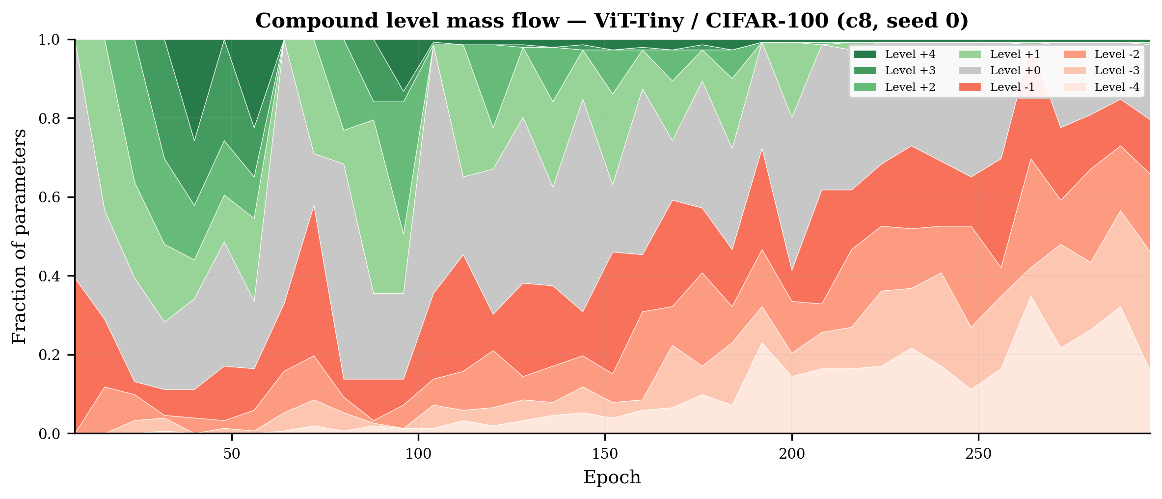
\(V_1 = -1\) (reversal detection) rises nearly monotonically from \(20\%\) in early training to \(56\%\) by epoch \(296\): as training progresses, epoch-to-epoch gradient direction stability decreases for an increasing fraction of layers. \(V_1 = +1\) (strong stability) correspondingly decays from \(5\%\) to \(1\%\). \(V_2\) shows no monotonic trend; its firings appear episodically at single-digit rates. This profile is what drives the downward level migration visible in the stacked area plot (Figure 5).
8.6.0.3 Relation to level changes.
Combined with the compound level dynamics (Figure 3, Table 3), the picture is: the dominant driver of negative compound level accumulation is Vote 1’s growing reversal detection rate, moderated by the tiebreaker whenever both local votes abstain (\(58.6\%\) of decisions) – typically resolving in favour of rate maintenance or reduction as validation loss ceases to improve monotonically.
8.7 Additional Compound Level Trajectories↩︎
8.7.0.1 ViT-Tiny/CIFAR-100, cadence 8.
| Layer type | ep8 | ep64 | ep120 | ep176 | ep232 | ep296 | Mult. |
|---|---|---|---|---|---|---|---|
| all_attn | \(-0.35\) | \(+0.06\) | \(-1.22\) | \(-1.75\) | \(-2.13\) | \(-2.06\) | \(0.40\times\) |
| all_mlp | \(-0.35\) | \(+0.12\) | \(-0.83\) | \(-1.55\) | \(-1.98\) | \(-1.98\) | \(0.41\times\) |
| all_norm | \(-0.48\) | \(+0.11\) | \(-0.36\) | \(-0.53\) | \(-1.22\) | \(-1.43\) | \(0.53\times\) |
| embed+patch | \(-0.28\) | \(+0.12\) | \(-1.28\) | \(-1.19\) | \(-2.19\) | \(-2.06\) | \(0.40\times\) |
| head+final_norm | \(-0.25\) | \(+0.88\) | \(-0.31\) | \(-0.50\) | \(-1.44\) | \(-1.19\) | \(0.59\times\) |
At cadence 8, the early-training trajectory differs: levels are near zero or slightly positive at epoch 64, indicating the system initially finds no strong signal for rate reduction with the longer voting window. By mid-training (epoch 120), differentiation emerges, and by epoch 296 the attention-vs-normalisation spread (\(0.63\) levels, LR ratio \(1.33\)) is comparable to cadence 4 (\(0.61\) levels, ratio \(1.32\)).
8.7.0.2 WRN-28-10/CIFAR-10, cadence 4.
| Layer group | ep4 | ep44 | ep84 | ep124 | ep164 | ep200 |
|---|---|---|---|---|---|---|
| conv0 | \(-0.12\) | \(-3.12\) | \(-3.00\) | \(-0.88\) | \(-1.50\) | \(-1.00\) |
| layer1 | \(+0.05\) | \(-2.37\) | \(-2.38\) | \(-2.13\) | \(-2.00\) | \(-1.68\) |
| layer2 | \(-0.02\) | \(-2.41\) | \(-2.67\) | \(-2.13\) | \(-1.83\) | \(-1.62\) |
| layer3 | \(-0.06\) | \(-1.98\) | \(-2.54\) | \(-1.20\) | \(-1.48\) | \(-1.84\) |
| fc | \(-0.50\) | \(-3.38\) | \(-2.06\) | \(-2.12\) | \(-1.31\) | \(-1.75\) |
| final_bn | \(+0.31\) | \(-3.00\) | \(-2.00\) | \(-1.75\) | \(-1.19\) | \(-1.81\) |
The three repeated block groups (layer1, layer2, layer3) show a spread of \(0.22\) levels at epoch 200, compared to \(0.61\) levels between attention and normalisation on ViT-Tiny. The smaller spread reflects the architectural uniformity of WideResNet’s residual groups.
8.8 Effective Learning Rate Fingerprint↩︎
8.9 Compound Level Mass Flow↩︎
8.10 Cadence Effect on Layer-Type Differentiation↩︎
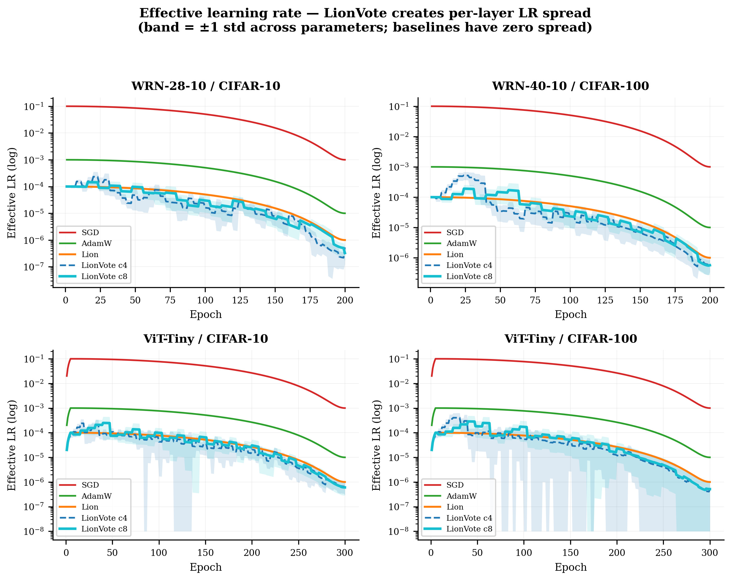
8.11 Effective Learning Rate Dynamics↩︎
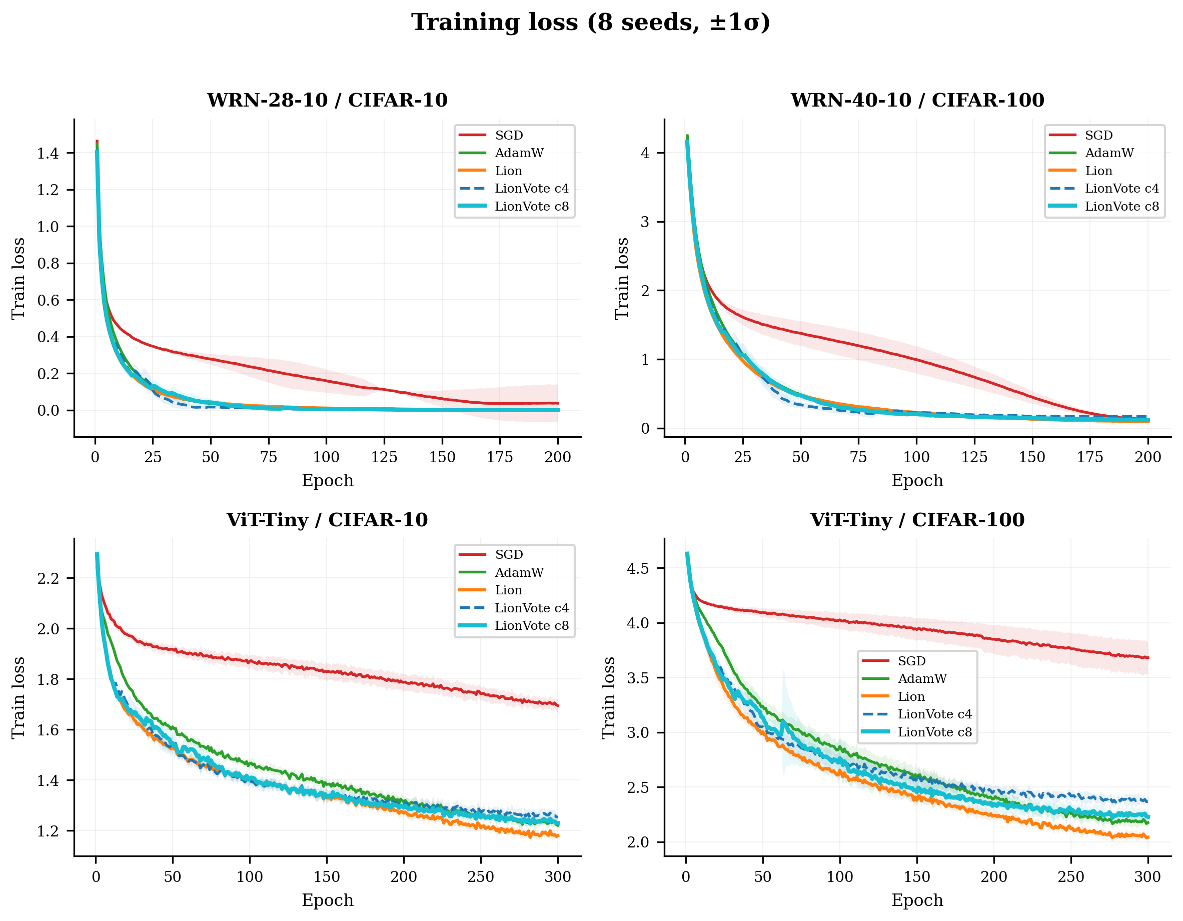
8.12 Training Loss Curves↩︎
8.13 Validation Loss Curves↩︎
8.14 Generalisation Gap↩︎
8.15 Control Experiments: Static Multipliers and Lower Base Rate↩︎
Four control baselines on ViT-Tiny/CIFAR-100 (8 seeds each, cosine warmup, 300 epochs) test whether the per-layer differentiation discovered by LionVote can be replicated by static means or by adjusting global hyperparameters.
8.15.0.1 Lion-Typed.
Lion with fixed per-layer-type LR multipliers from epoch 1, using the exact epoch-300 values from Table 3 (cadence 4): attention \({\times}0.38\), MLP \({\times}0.36\), normalisation \({\times}0.50\), embedding \({\times}0.40\). Base \(\mathrm{lr}{=}10^{-4}\), \(\mathrm{wd}{=}0.5\).
8.15.0.2 Lion (\(\mathbf{lr{=}4{\times}10^{-5}}\)).
Plain Lion at \({\sim}2.5{\times}\) lower base rate, matching LionVote’s average effective rate at convergence. \(\mathrm{wd}{=}0.5\).
8.15.0.3 Weight decay sweep.
Lion at \(\mathrm{wd}{=}0.25\) (\(0.5{\times}\) default) and \(\mathrm{wd}{=}0.75\) (\(1.5{\times}\) default), both with \(\mathrm{lr}{=}10^{-4}\).
All \(p\)-values are Welch two-sample \(t\)-tests (\(n = 8\) per group).
| Method | Accuracy (%) | \(\Delta\) vs.Lion | Welch \(p\) vs.Lion |
|---|---|---|---|
| LionVote (c8) | \(69.71 \pm 0.60\) | \(+0.76\) | \(0.012\) |
| Lion (\(\mathrm{wd}{=}0.25\)) | \(69.12 \pm 0.58\) | \(+0.17\) | \(0.52\) |
| Lion (\(\mathrm{lr}{=}10^{-4}\)) | \(68.95 \pm 0.41\) | — | — |
| Lion (\(\mathrm{wd}{=}0.75\)) | \(68.91 \pm 0.31\) | \(-0.04\) | \(0.84\) |
| Lion (\(\mathrm{lr}{=}4{\times}10^{-5}\)) | \(68.72 \pm 0.45\) | \(-0.23\) | \(0.30\) |
| Lion-Typed | \(68.47 \pm 0.34\) | \(-0.48\) | \(0.024\) |
Lion-Typed is significantly worse than standard Lion (\(-0.48\) pp, \(p = 0.024\)) but not significantly worse than AdamW (\(-0.28\) pp, \(p = 0.15\)). The lower-LR control is statistically indistinguishable from Lion (\(p = 0.30\)) and from AdamW (\(p = 0.89\)). The two controls are indistinguishable from each other (\(p = 0.23\)), and both are significantly below LionVote at cadence 8 (\(p = 0.003\) and \(p < 0.001\) respectively). Neither weight decay variant significantly differs from the default: \(\mathrm{wd}{=}0.25\) is the best static variant but remains \(0.59\) pp below LionVote at cadence 8 (\(p = 0.075\)).
8.15.0.4 Per-seed accuracy.
| Seed | Lion-Typed | Lion (\(4{\times}10^{-5}\)) | LionVote (c8) |
|---|---|---|---|
| 2 | 68.60 | 68.81 | 70.44 |
| 18 | 68.15 | 68.96 | 69.54 |
| 20 | 68.01 | 68.09 | 69.29 |
| 26 | 68.92 | 68.88 | 69.89 |
| 40 | 68.84 | 69.38 | 68.95 |
| 44 | 68.46 | 68.35 | 70.84 |
| 48 | 68.66 | 69.06 | 69.26 |
| 52 | 68.16 | 68.24 | 69.45 |
No Lion-Typed seed exceeds \(69\%\); one lower-LR seed (of eight) exceeds \(69\%\); seven of eight LionVote seeds exceed \(69\%\).
8.15.0.5 Convergence speed.
| Threshold | Lion (\(4{\times}10^{-5}\)) | Lion-Typed | Lion (\(10^{-4}\)) | LV c8 | AdamW |
|---|---|---|---|---|---|
| \(63\%\) | 68 | 71 | 85 | 76 | 121 |
| \(65\%\) | 103 | 104 | 130 | 100 | 158 |
| \(67\%\) | 187 | 188 | 199 | 133 | 214 |
| \(68\%\) | 240 | 253 | 239 | 160 | 250 |
| \(69\%\) | 2/8 | 0/8 | 3/8 | 7/8 | 3/8 |
Both controls converge faster than Lion (\(10^{-4}\)) and AdamW to early thresholds (\(63\)–\(67\%\)) but plateau lower. LionVote at cadence 8 reaches \(68\%\) at epoch \(160\), a full \(80\) epochs before the lower-LR control.
8.15.0.6 Per-seed accuracy: ablation variants and WD sweep (ViT/C100, cadence 8).
| Seed | v1only | notie | symmetric | Lion (wd=0.25) | Lion (wd=0.75) |
|---|---|---|---|---|---|
| 2 | 68.86 | 68.54 | 70.26 | 69.43 | 69.15 |
| 18 | 69.21 | 69.35 | 71.27 | 69.67 | 69.28 |
| 20 | 68.03 | 68.17 | 70.43 | 68.35 | 68.93 |
| 26 | 67.79 | 67.65 | 68.86 | 68.53 | 68.49 |
| 40 | 69.11 | 68.94 | 70.69 | 70.02 | 69.22 |
| 44 | 68.42 | 68.81 | 72.15 | 69.18 | 69.02 |
| 48 | 68.55 | 68.81 | 70.49 | 69.08 | 68.54 |
| 52 | 68.57 | 68.85 | 70.18 | 68.68 | 68.68 |
| Mean | 68.57 | 68.64 | 70.54 | 69.12 | 68.91 |
| Std | 0.49 | 0.52 | 0.94 | 0.58 | 0.31 |
8.16 Raw Lion Gradient Diagnostics (No Voting Mechanism)↩︎
To test whether the layer-type differentiation observed in §5.1 is an artefact of LionVote’s specific voting mechanism, the same per-layer diagnostics were measured during standard Lion training on ViT-Tiny/CIFAR-100 (seed 2, cadence 8 measurement interval, cosine warmup, 300 epochs). No voting, no compound levels, no per-layer LR adjustment—only the raw diagnostic signals.
8.16.0.1 Gradient direction stability.
Table 15 reports the mean epoch-mean cosine alignment \(c_i = \cos(\bar{g}_i^{(\mathrm{curr})}, \bar{g}_i^{(\mathrm{prev})})\) by layer type in late training (epoch \(\geq 200\)).
| Layer type | Mean cosine | Std | Would vote \(-1\) | Abstain | Would vote \(+1\) |
|---|---|---|---|---|---|
| attn | \(-0.005\) | \(0.106\) | \(56\%\) | \(43\%\) | \(<1\%\) |
| mlp | \(-0.002\) | \(0.054\) | \(56\%\) | \(44\%\) | \(0\%\) |
| norm | \(+0.104\) | \(0.192\) | \(30\%\) | \(69\%\) | \(1\%\) |
Under standard Lion, attention and MLP layers have mean cosine alignment near zero: their epoch-mean gradients are essentially uncorrelated across consecutive measurement windows. Normalisation layers have mean cosine \(+0.104\)—substantially higher, indicating more directionally stable gradients. Attention and MLP parameters would receive a negative vote (cosine \(< 0\)) on \(56\%\) of measurement epochs, compared to \(30\%\) for normalisation—a \(1.9{\times}\) ratio. This asymmetry in raw gradient statistics is the signal that LionVote’s Vote 1 detects; it exists in standard Lion training independent of the voting mechanism.
8.16.0.2 Momentum health.
The momentum-to-gradient norm ratio \(r = \|m\| / \|\bar{g}\|\) stays within the Vote 2 dead zone \([1/e, e]\) for \(98\)–\(100\%\) of measurements across all layer types, confirming that Vote 2’s low firing rate (§4.3) reflects the training dynamics, not the threshold placement.
8.16.0.3 Cross-optimizer comparison (Lion vs.AdamW).
Running the same diagnostics under AdamW (ViT-Tiny/CIFAR-100, cosine warmup, lr\({=}10^{-3}\), wd\({=}0.05\), single seed) reveals that the attn \(<\) norm ordering is optimizer-general, but Lion amplifies the gap.
| Mean cosine \(\pm\) std | Negative-vote rate | |||
|---|---|---|---|---|
| 2-3(lr)4-5 Layer type | Lion | AdamW | Lion | AdamW |
| attn | \(-0.005 \pm 0.106\) | \(-0.005 \pm 0.097\) | \(56.4\%\) | \(56.1\%\) |
| mlp | \(-0.002 \pm 0.054\) | \(+0.001 \pm 0.056\) | \(56.4\%\) | \(54.3\%\) |
| norm | \(+0.104 \pm 0.192\) | \(+0.053 \pm 0.161\) | \(29.8\%\) | \(37.5\%\) |
| other | \(+0.081 \pm 0.216\) | \(+0.027 \pm 0.183\) | \(30.8\%\) | \(55.8\%\) |
| norm–attn gap | \(0.109\) | \(0.058\) | ||
The attn \(<\) norm ordering holds for both optimizers (\(100\%\) of late epochs under Lion, \(92\%\) under AdamW), confirming the heterogeneity is architectural. Lion’s \(\operatorname{sign}(\cdot)\) amplifies the norm–attn cosine gap \(1.88{\times}\) relative to AdamW (\(0.109\) vs.\(0.058\)): because sign discards gradient magnitude, directionally unstable layers cannot compensate through large gradients. AdamW’s second moment (\(1/\sqrt{\hat{v}}\)) implicitly down-weights noisy coordinates, partially absorbing the layer-type difference. This explains why per-layer correction has the largest marginal value for sign-based optimizers: no within-update self-correction mechanism exists.
8.16.0.4 Vote 2 under AdamW: thresholds are Lion-specific.
The cosine-alignment comparison above concerns only Vote 1’s input signal. The analogous comparison for Vote 2 – the momentum-to-gradient norm ratio \(r = \|m\|/\|\bar{g}\|\) – reveals a qualitative difference. Under Lion, \(r\) has geometric mean \({\sim}1.8\) across layer types and sits within the dead zone \([1/e, e]\) for \({\sim}97.6\%\) of observations (Table 17). Under AdamW with the same parameters monitored, \(r\) has geometric mean \({\sim}8\)–\(10\) and lies above \(e\) for \({\sim}100\%\) of observations.
| Geo.mean \(r\) by layer | Overall \(V_2\) | |||
|---|---|---|---|---|
| 2-3(lr)4-5 Layer / Stat | Lion | AdamW | Lion | AdamW |
| attn | \(1.898\) | \(9.384\) | — | — |
| mlp | \(1.790\) | \(8.022\) | ||
| norm | \(1.769\) | \(8.818\) | ||
| other | \(1.914\) | \(9.930\) | ||
| \(V_2 = +1\) rate | \(0.00\%\) | \(0.00\%\) | ||
| \(V_2 = 0\) rate | \(97.57\%\) | \(0.02\%\) | ||
| \(V_2 = -1\) rate | \(2.43\%\) | \(99.98\%\) | ||
The ratio difference is a consequence of the different momentum mechanics. Lion’s \(\beta_2\) outer EMA (\(\beta_2 = 0.99\) default) smooths the update buffer over roughly \(100\) steps, keeping its norm comparable to the current gradient. AdamW’s first-moment EMA with \(\beta_1 = 0.9\) accumulates raw gradients on a much longer effective horizon when unnormalised by the second moment (which is applied separately by division inside the update itself rather than to the buffer we monitor), so the buffer norm significantly exceeds the current-gradient norm on this workload. Consequently, Vote 2’s symmetric \([1/e, e]\) dead zone – which is derived from the EMA time-constant identity \(\beta_2^{\tau} = e^{-1}\) – is calibrated against Lion’s \(\beta_2\)-EMA and produces a near-constant \(V_2 = -1\) signal under AdamW, making it useless for per-layer modulation without recalibration.
8.16.0.5 Optimizer-agnostic versus Lion-specific components.
Combining the Vote 1 comparison (near-invariant between Lion and AdamW: \(V_1 = -1\) rate \(37.6\%\) vs.\(35.4\%\); \(V_1 = +1\) rate \(2.5\%\) vs.\(1.1\%\)) with the Vote 2 comparison (optimizer-dependent: dead-zone occupancy \(97.6\%\) vs.\(0.02\%\)), the LionVote mechanism decomposes as follows:
| Component | Portability notes |
|---|---|
| \(V_1\) input (cosine of epoch-mean gradients) | Optimizer-agnostic: gradient-only statistic. |
| \(V_1\) upper threshold \(0.5\) | Sheppard derivation (App. [sec:app:vote1]) uses the sign-update structure; the \(2/3\) convention is optimizer-agnostic. |
| \(V_1\) lower threshold \(0\) | Optimizer-agnostic: parameter-free geometric identity. |
| \(V_2\) input \(\|m\|/\|\bar{g}\|\) | Optimizer-agnostic: computable from any momentum-based optimizer. |
| \(V_2\) thresholds \(1/e\), \(e\) | Lion-specific: calibrated to Lion’s \(\beta_2\)-EMA time constant; misfire under AdamW’s different momentum structure. |
| Tiebreaker (validation \(\pm 1\%\)) | Optimizer-agnostic: loss-based. |
| LR exponent numerator \(\beta_1\) | Lion-specific form: Lion’s \(\beta_1\) is the momentum-gradient interpolation coefficient; other optimizers use \(\beta_1\) differently. |
| LR exponent divisor \(2\) | Derived from the sign-based descent lemma (App. [sec:app:exponent]); the principle transfers but the exact coefficient requires per-optimizer re-derivation. |
| Compound-level integer state machine | Optimizer-agnostic: generic over votes (Algorithm [alg:lionvote]). |
| Cadence \(c\), max level \(L\) | Optimizer-agnostic: generic hyperparameters. |
Two components are essentially Lion-specific: Vote 2’s thresholds (empirically demonstrated above) and the LR exponent’s numerator \(\beta_1\) (by Lion’s specific use of \(\beta_1\) as the momentum-gradient interpolation coefficient). Three components are optimizer-agnostic in input and require only Lion’s sign-update structure for one of the two derivations on their thresholds: Vote 1, the tiebreaker, and the compound-level state machine. The divisor \(2\) principle transfers but the coefficient may not. A port to another momentum-based optimizer would therefore preserve the architecture of the voting mechanism, recalibrate Vote 2 using that optimizer’s effective momentum time constant, and re-examine the LR exponent. We do not carry out such a port; this is left to future work.
8.16.0.6 Single-seed limitation.
These measurements (Vote 1, Vote 2, and Lion/AdamW cross-optimizer comparisons above) are from a single seed. The layer-type ordering (norm more stable than attn/mlp) is consistent with the 8-seed compound level trajectories in Table 3 and the structural argument in §5.1. The Vote 2 dead-zone discrepancy between Lion and AdamW reflects a single-seed observation of an effect (\({\sim}5{\times}\) ratio difference) whose magnitude far exceeds plausible seed-to-seed variation and is therefore unlikely to reverse under replication, though confirming this is left to future work.
8.17 Partial Schedule Replacement↩︎
LionVote without any global schedule outperforms the scheduled variant on WRN/C10 at cadence 8 by \(0.18\) pp (\(93.48\%\) vs.\(93.30\%\)), though this difference is not statistically significant given the standard deviations (\(\pm 0.39\) vs.\(\pm 0.82\)). It falls short by \(0.82\) pp on ViT/C100 (\(68.89\%\) vs.\(69.71\%\); Table 2). The universally negative compound levels implement a form of learning rate decay that overlaps in function with cosine annealing. On architectures where this overlap is sufficient (WRN), the schedule becomes unnecessary; on ViTs, the schedule provides additional value.
8.18 Computational Cost Details↩︎
LionVote adds one in-place gradient accumulation per parameter per batch and linear voting cost (one cosine similarity, one norm ratio, one integer comparison per parameter) every \(c\) epochs. No second-order information, meta-gradients, or additional forward/backward passes are required. Memory overhead beyond Lion is two tensors per parameter (the gradient accumulator and the previous epoch-mean gradient snapshot) plus two scalars (the compound level and the effective learning rate). The per-batch accumulation is a single in-place addition per parameter (the same operation count as one line of Lion’s momentum update) and is negligible relative to the forward/backward pass. Voting fires once every \(c\) epochs; for ViT-Tiny (\(152\) parameter tensors), this is \(152\) dot products and norms. The dominant overhead is memory: the two extra tensors triple Lion’s per-parameter optimizer state (\({\sim}23\) MB for Lion, \({\sim}69\) MB for LionVote on ViT-Tiny). For billion-parameter models the \(3{\times}\) increase is a deployment concern.
8.18.0.1 Hardware and total compute.
All experiments were run on a single NVIDIA GPU (A100, T4, or L40S depending on availability). The 605 runs reported in this paper required \({\sim}901\) GPU-hours in total:
| Configuration group | Runs | Total (hrs) | Avg per run (min) |
|---|---|---|---|
| WRN-28-10 / CIFAR-10 | 285 | 417 | 88 |
| WRN-40-10 / CIFAR-100 | 88 | 176 | 120 |
| ViT-Tiny / CIFAR-10 | 88 | 72 | 49 |
| ViT-Tiny / CIFAR-100 | 112 | 146 | 78 |
| Controls (ViT/C100) | 32 | 90 | 168 |
| Total | 605 | 901 | — |
No preliminary or failed experiments beyond those reported were conducted.