Co-evolution of self-replication and function in a digital primordial soup
July 10, 2026
Abstract
While traditional evolutionary algorithms hard-code reproduction, self-replication can emerge spontaneously within digital “primordial soups”. This paper investigates the co-evolution of this emergent self-replication alongside problem-solving capabilities. We initialize a population of random 32-byte Z80 assembly programs, requiring self-replication to arise purely through random assembly-level mutations and pairwise program interactions. To link these behaviors, we introduce a task-based validation step: correctly evaluating a polynomial raises a program’s interaction probability above a baseline rate. Our experiments yield four primary findings. First, self-replication and mathematical problem-solving successfully co-evolve from initial randomness. Second, the pressure to compute accelerates the emergence of compact, robust reproductive architectures that preserve memory for task execution. Third, applying metabolic constraints increases the likelihood that programs evolve conditional halting, terminating early during validation while bypassing the halt during interaction to execute block-copy replication. Finally, when programs are partitioned into spatial task niches, spontaneous self-replication generates an emergent learning curriculum, utilizing simple solutions as stepping stones toward complex polynomials. Altogether, these results demonstrate an interactive feedback loop: environmental task demands actively shape the physical architecture of self-replication, while spontaneous replication alters the evolutionary trajectory of functional problem-solving.
1 Introduction↩︎
Origin of life research has long debated the fundamental drivers required for life to emerge from non-living matter [1]. Genetics-first accounts hold that life began with self-replicating, information-bearing molecules [2], whereas metabolism-first accounts posit that energy-harnessing autocatalytic networks preceded genetic replication [3]–[7]. A complementary tradition treats the two as jointly necessary, with frameworks such as Gánti’s chemoton [8] and Dyson’s double-origin hypothesis [9] positing that a minimal living system must couple metabolism with replication. This inquiry extends naturally into Artificial Life (ALife), which seeks to explore the universal principles of living systems across abstract computational substrates [10]–[13]. Across both biological and digital domains, the spontaneous emergence of self-replication marks a critical phase transition from pre-evolutionary interactions to Darwinian evolution [14]–[16]. However, platforms studying the evolution of complex behaviors—whether via cellular automata, agentic simulators, or assembly-language organisms—typically bypass the stochastic hurdles of this transition by hard-coding reproduction or seeding their environments with hand-crafted ancestral replicators [17]–[33].
To bridge the gap between pre-life emergence and life-era evolution, it is vital to study environments where reproduction is not an axiomatic guarantee. While early ALife models [34]–[36] and recent studies [15] have successfully demonstrated that self-replicating programs can spontaneously emerge from random, unseeded initializations without explicit fitness landscapes, these works generally do not explore the essential next step: the evolution of complex problem-solving. In this paper, we build directly upon the foundational digital primordial soup framework of [15] to link the spontaneous emergence of reproduction to the evolution of complex algorithmic behaviors. Specifically, we investigate how the capacity to solve increasingly complex mathematical tasks co-evolves alongside the spontaneous origination of reproduction itself.
We explore this by situating a population of random programs on a spatial grid where each entity is a Z80 assembly program executed by an emulated microprocessor. Here, reproduction is not a system-level command, but a behavior that must be discovered through the execution of assembly instructions. To investigate the relationship between primordial reproduction and complex problem-solving, we introduce a competence-gated interaction rule. Under this regime, a program’s opportunity to execute and potentially reproduce is contingent upon a validation step: the program is challenged to evaluate a specific mathematical polynomial. The instruction set lacks a native multiplication instruction, requiring the evolution of complex iterative loops to perform polynomial evaluation, thus presenting a rugged algorithmic search space. This setup differs significantly from platforms such as Avida [29]–[31], where solving a task can be viewed as a form of computational metabolism [37] that is rewarded with the execution of a built-in copy command, thereby explicitly binding competence and reproduction together. Crucially, our system instead decouples the two: a successful polynomial evaluation merely increases the likelihood that a program will receive an opportunity to interact with its neighborhood, and does not facilitate or trigger replication. For a lineage to persist in our model, therefore, it must satisfy two independent conditions: the program must pass the validation step and it must also possess its own evolved mechanism for self-replication. Solving the task is therefore insufficient for propagation if the program does not simultaneously encode the instructions required to copy itself into the available memory space.
Our experiments yield four primary findings that highlight the interaction between emergent reproduction and the evolution of task solutions. First, we find that self-replication and task-solving co-evolve within individual programs. Replication is a strict prerequisite for propagation: a task solution cannot spread through the population unless the program carrying it can also copy itself. Task-solving is not strictly required to reproduce, but it confers a selective advantage, since a program that solves its task is far more likely to be selected for interaction than one that does not. Under this combined pressure, robust and efficient reproductive architectures reliably emerge from random noise and, in the same programs, acquire the ability to solve mathematical tasks of increasing complexity. This joint emergence establishes the platform for the three findings that follow.
Second, we find that the pressure to solve tasks reshapes the way the reproductive machinery itself evolves. The earliest replicators to emerge copy themselves by devoting nearly the entire program to the reproduction operation, leaving no room for the instructions needed to solve a task. More compact replication mechanisms occupy just a few bytes and leave the rest of the tape free, so that the same program can both reproduce and compute. Because these compact replicators can do both, the demand to solve tasks accelerates the population’s transition toward them. In short, the pressure to solve tasks feeds back onto the architecture of how a program reproduces.
Third, we show that if we apply a metabolic constraint to the task solutions [38] (i.e. we decrease a program’s chance to interact based on how many operations it uses to solve a task), then the programs evolve conditional operations to distinguish between task solution runs and program interaction runs.
Finally, we find that the dynamics of reproduction influence the evolution of task solutions. Specifically, we find that in unstructured (panmictic) environments, where programs interact freely with any other programs, populations consistently fail to compute high-degree polynomials. We demonstrate that this failure is an instance of the objective paradox [39], [40], in which explicitly rewarding progress deceives the search and explains why a smoothed fitness landscape fails to aid discovery. Rather, we demonstrate that the emergence of programs computing high-degree polynomials is reliably observed only when the grid is partitioned into distinct task niches, coupled with sparse migration [41], [42]. We show that this spatial structure generates an emergent curriculum, utilizing previously solved simpler tasks as genetic stepping stones for higher-complexity tasks. Altogether, these results demonstrate that self-replication and the ability to solve tasks of increasing complexity co-evolve. As well, pressure to solve complex tasks can influence the emergence and mechanics of spontaneous reproduction, and in turn, the presence of niches for reproduction can help to shape task solutions through emergent curricula.
2 Results↩︎
2.1 Model overview↩︎
To study the co-emergence of self-replication and task solving, we create a population of random programs across a set of separate niches, each assigned a different mathematical task. Evolution proceeds through repeated epochs, in which programs are mutated, tested on their niche’s task, and paired for interaction. Solving the task makes a program more likely to be selected for interaction, and when two programs interact, one program can run assembly instructions that copy its own bytes over those of the other. Because an interaction overwrites the two programs with its result, a program that copies itself spreads through the substrate, while one that does not tends to be overwritten by those that do.
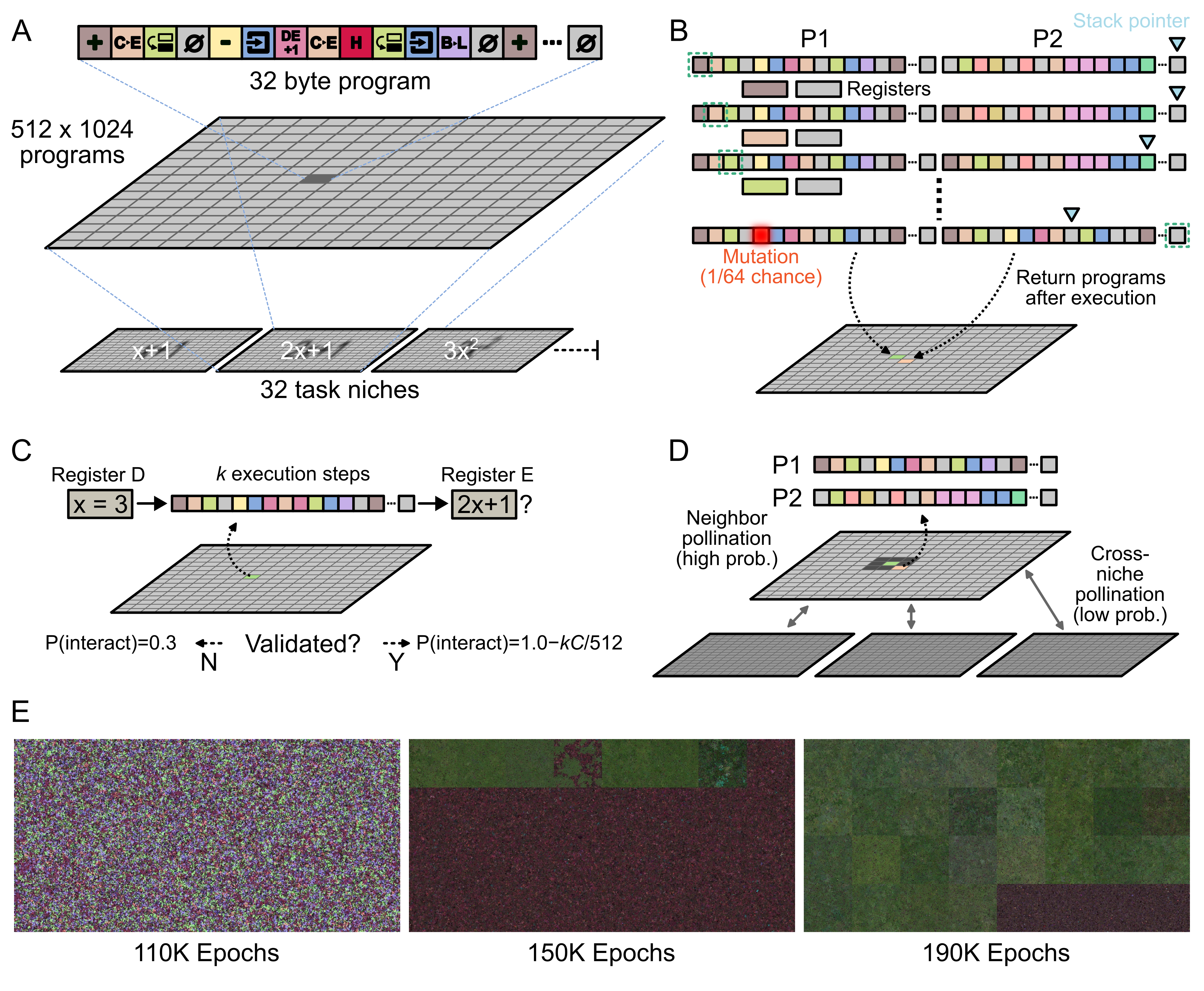
Concretely, the population is divided into 32 niches, and each niche is a separate two-dimensional grid of cells, with one program per cell. A program is a sequence of \(\ell = 32\) bytes, which we also call a “tape” (Fig. 1A). Within a niche, position matters, because a program interacts mostly with its immediate neighbors on the grid. The niches have no spatial arrangement relative to one another, so they act as a collection of separate populations. Each niche is assigned one of 32 polynomial functions, and a program’s task is to evaluate the polynomial of its niche. Across all niches the population totals \(2^{19}\) programs, all initialized as random byte sequences.
Each epoch begins with a mutation step, in which every program has a small chance of having one random byte reinitialized (Fig. 1B). The programs are then evaluated, and a subset is selected for pairwise interaction, as we describe next.
The program evaluation is a competence test we call “validation”. The program is run on its own by a Z80 emulator (see for details), and we check whether it evaluates its niche’s polynomial correctly on a few randomly sampled inputs. This validation yields a binary success or failure signal, meaning the program passes only if it computes the correct output for all sampled inputs. Executing a program writes its final memory state back to its cell, so any modification it makes to its own bytes during validation persists, just as it does during an interaction.
A program that passes validation becomes much more likely to be selected for interaction, though this likelihood is reduced by a metabolic penalty that grows with the number of steps it used to pass the validation (Fig. 1C). A program that fails is still selected sometimes, but only at a low baseline rate (see for the exact rule).
A selected program is then paired with a partner. Most of the time, with probability \(0.95\), the partner is one of its immediate neighbors in the same niche. The rest of the time the partner is any program drawn uniformly from the whole population (Fig. 1D). This occasional long-range pairing, which we call cross-niche pollination (CNP), lets a solution found in one niche spread into another, and we show later that it is key for solving the harder tasks.
In an interaction, the two programs’ tapes are concatenated into a single \(2\ell\)-byte memory space, and execution begins at the first byte of the first program. Replication is never imposed by the system; it occurs only when the executed code, on its own, copies one program’s bytes over the second program’s memory region. Whatever the combined tape contains at the end of a fixed instruction budget is split back into two 32-byte halves and written back into the cells the two programs came from, carrying the result into the next epoch.
2.2 Self-reproduction and task solutions emerge from a primordial soup↩︎
Over one million epochs of evolution, robust self-replication and task-solving capabilities consistently co-emerged from completely random initial programs, as successful self-replicating lineages spread to dominate the grids (Fig. 1E). This result shows that spontaneous replication and the ability to solve increasingly complex tasks can co-evolve. Indeed, the two abilities reinforce each other. A program that cannot replicate is inevitably overwritten by one that can, regardless of its task-solving competence. Conversely, among replicating programs, those that successfully solve their niche’s polynomial are selected for interaction at a higher rate. Over time, the lineages that dominate a niche tend to integrate both behaviors.
In contrast to a standard evolutionary algorithm, our system never copies or reproduces programs. It provides only random initialization, mutation, and a validation step that biases how frequently programs interact. This bias induces a fitness landscape, but the system offers immediate no means of climbing it, since reproduction must be discovered by the executed code. The evolutionary machinery therefore emerges from random bytes together with the ability to solve problems, rather than being supplied in advance.
2.3 Tasks alter the dynamics of emergent self-replication↩︎
The co-emergence of replication and task-solving raises a natural question: how do the two interact as evolution proceeds? One might expect a simple sequence, in which a replicator is discovered, replicates until it dominates the population, and only
afterwards evolves to solve tasks. Instead, we found a more intricate coupling, in which the pressure to solve tasks and the architecture of replication shape one another. Two types of replicators came to dominate the population at different epochs. The
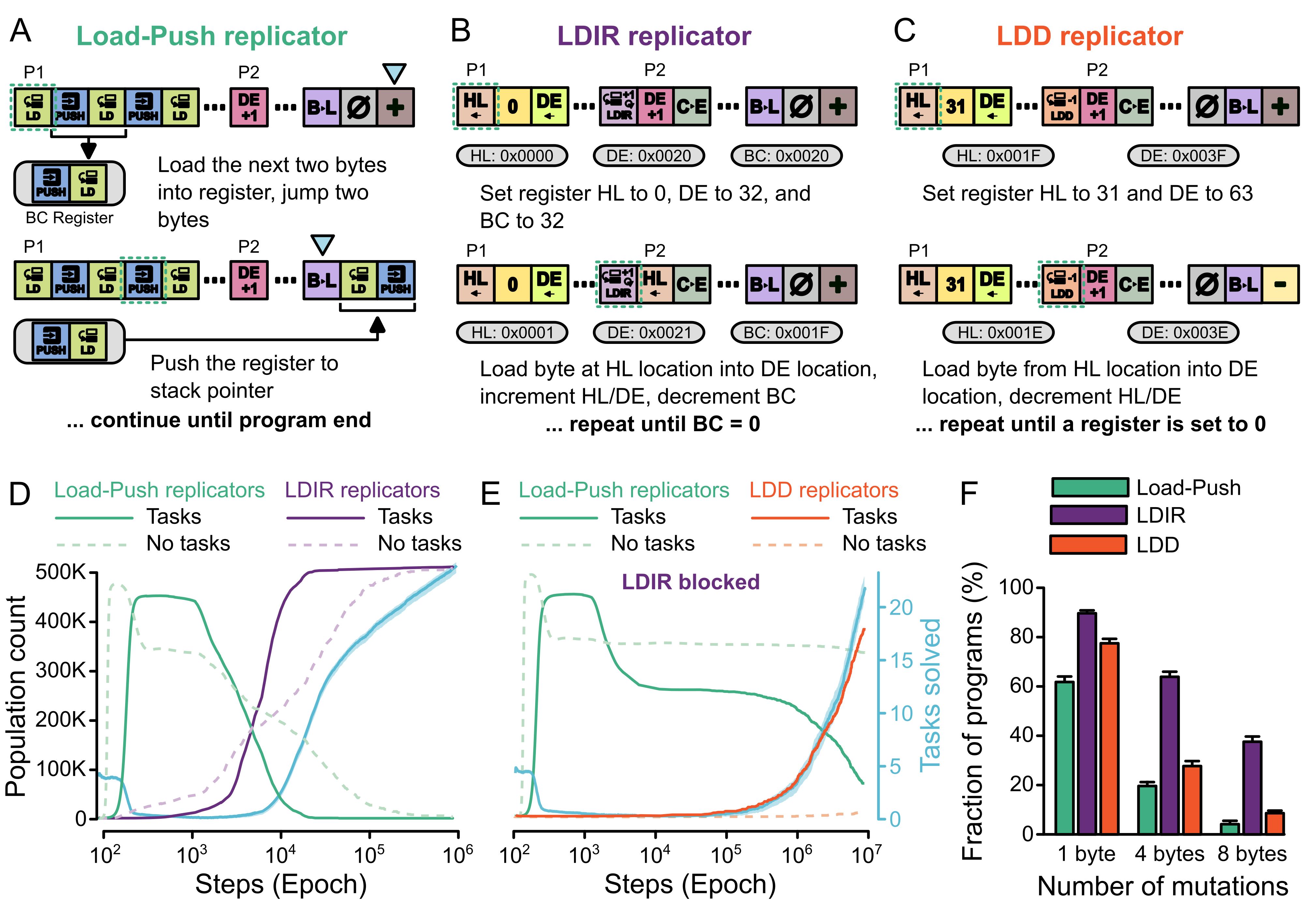
first, a simple replicator we call ‘Load-Push’, consists of a string of paired ‘Load’ and ‘Push’ instruction bytes. Because the Z80’s PUSH instruction operates on 16-bit registers, each pair copies the program two bytes at a time to the
adjacent memory space of a partner program (Fig. 2A). Lacking a loop, full replication requires a long chain of these pairs, meaning a Load-Push replicator consumes the entire 32-byte tape.
A second replicator, the ‘Load Increment Repeat’ (LDIR) replicator, reliably took over later. It utilizes a specialized Z80 block-copy instruction (LDIR) that automatically loops to copy a sequence of bytes from one location in memory to
another. Rather than a long, repetitive sequence of instructions, it needs only to initialize its copy parameters to copy from P1 into P2 once before the single instruction executes the entire copy. This allows a program to achieve replication using only a
few bytes (Fig. 2B), leaving the rest of its memory free for task-solving code (see for the exact register mappings).
As noted above, the Load-Push replicators were the first to appear and dominate the grids (Fig. 2D, solid green line), but they eventually gave way to the LDIR replicators (Fig. 2D, solid purple line). The number of tasks solved tracked this turnover (Fig. 2D, solid blue line). Specifically, the number of tasks solved dropped as the Load-Push replicators spread, then recovered and grew as the LDIR replicators took over. The reason for this dynamic is that a Load-Push replicator uses the entire tape to copy itself, leaving no room for task-solving code, so its spread displaces programs that solve tasks. The LDIR replicator, by contrast, needs only a few bytes and leaves the rest of the program free; accordingly, its emergence always preceded the growth in task-solving programs, indicating that it unlocked the ability to both replicate and solve tasks. Consistent with this, removing the task-based gating of interactions (see for details) slowed the Load-Push-to-LDIR transition but did not prevent it (Fig. 2D, dotted line). The transition is intrinsically driven by differences in mutational robustness among the replicators (which we quantify below), with tasks serving to accelerate it.
To determine whether the accelerating effect of task pressure is specific to the LDIR instruction, we ran control experiments where we removed LDIR and its close relatives (LDI and LDDR) from the
language. In their absence, we observe the consistent emergence of a different replication mechanism based on the LDD instruction, though it takes over the population much more slowly than LDIR had (Fig. 2E, solid lines). This transition occurs consistently only under task pressure; without it, the transition from Load-Push is extremely slow and fails to complete within one million epochs (Fig. 2E, dashed lines). While LDIR has a built-in repeat mechanism that copies the entire program once its parameters are initialized, LDD copies only a single byte at a time. An LDD-based replicator must
therefore not only initialize its parameters to copy from P1 to P2 but it also must implement an explicit, multi-byte loop to achieve replication (Fig. 2C), representing a more complex reproductive architecture.
These results show that when one solution for reproduction is blocked, another is found, and that task pressure again accelerates the change. To verify our hypothesis that LDIR replicators naturally come to dominate because there is a
robustness hierarchy of the replicators, we quantified how well each reproduction architecture tolerates replication errors (see ). Our measurements revealed a clear robustness hierarchy (LDIR \(>\) LDD \(>\) Load-Push), where LDIR programs remain functional after successive mutations significantly more often than LDD loops, which in turn outperform the Load-Push sequences (Fig. 2F).
Taken together, these experiments show that the way a program reproduces keeps evolving after self-replication first appears. Robustness to mutation drives the population toward more compact replicators on its own, but the pressure to solve mathematical tasks accelerates that shift, because a compact replicator leaves room in the tape for task-solving code needs. The fitness landscape created by the tasks thus reshapes the replication machinery, so that how a program computes and how it reproduces evolve together.
2.4 Metabolic constraints drive efficient, conditional execution↩︎
In biological systems, computation is not free; organisms must balance the energy spent processing information with the resources required for replication. To study how such efficiency constraints shape algorithmic evolution, we introduced a “metabolic cost” to the validation phase, discounting a program’s interaction probability in proportion to the number of execution steps it takes to solve its task (see ). We asked whether this constraint would drive the evolution of more efficient programs, and how it might affect the replication phase where the constraint does not apply.
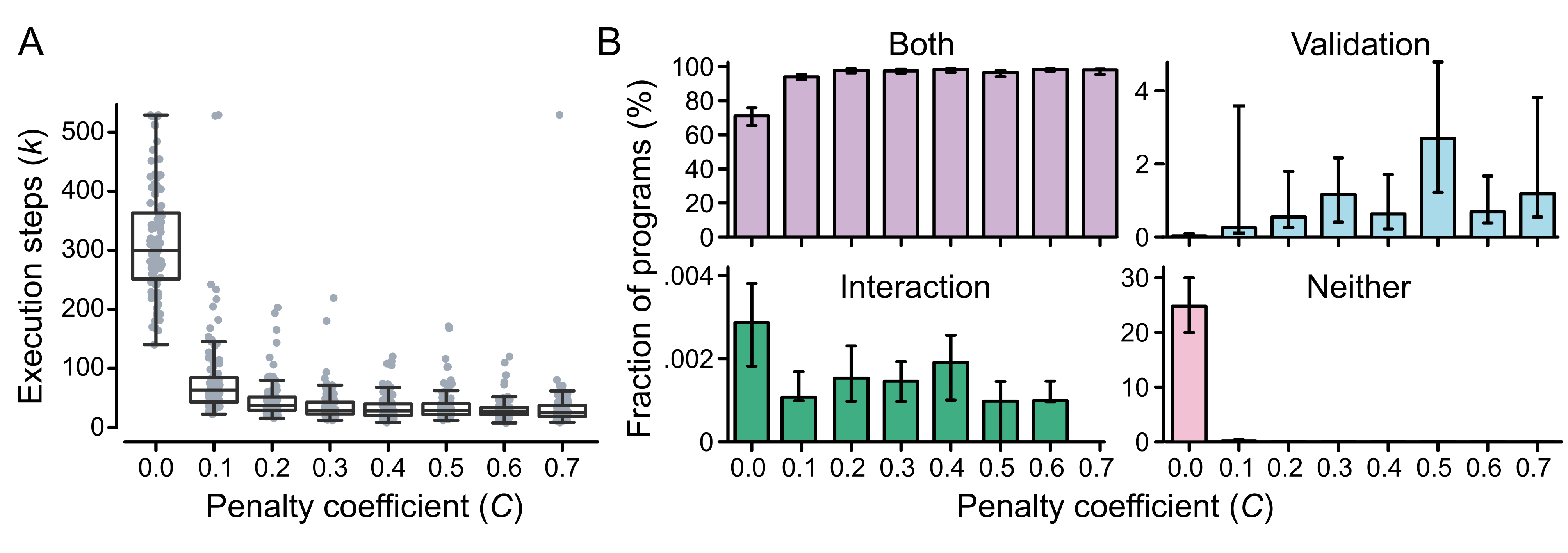
While the metabolic constraint left the overall rate of task solution emergence unchanged, it profoundly altered how those solutions were implemented. As the metabolic penalty coefficient increased, the average number of execution steps spent during
validation fell significantly (Fig. 3A). This efficiency was achieved because evolved programs consistently began incorporating a HALT instruction, which terminates execution as soon as the correct
output is computed.
In a minority of simulations, programs went further, evolving context-dependent behavior by exapting register D as a sensory cue to distinguish between the validation and interaction phases. In our execution protocol, the emulated
environment uses register D to pass the task input \(x \in \{0,\ldots,15\}\) during validation, meaning it contains a non-zero value fifteen times out of sixteen. During the interaction phase, however, the
environment always initializes D to zero. Evolving programs occasionally co-opted this difference, executing a conditional branch that triggers a HALT instruction only when the value in D is non-zero. Although this
conditional halting remained a minority strategy in absolute terms, the probability of its emergence rose significantly as the metabolic penalty became more severe (Fig. 3B).
This behavior represents a case of one evolved sequence serving two distinct roles depending on the environmental context. Because the same program is executed during both validation and interaction, the metabolic pressure on computation (the task-solving phase) can shape how the program behaves during reproduction (the interaction phase), even though the reproductive step itself carries no metabolic penalty. This provides a further example of how computation and reproduction can become coupled within a single, short program.
2.5 Cross-niche pollination produces emergent curricula↩︎
To evaluate the learning capabilities of a system where reproduction and problem-solving co-evolve, we tested its capacity to solve tasks of increasing complexity. In our system, solving higher-order polynomials depended crucially on the spatial organization of the population. When programs were structured into niches that exchanged material sparsely through cross-niche pollination, solutions to simpler tasks could seed niches working on harder ones. This spatial structure allowed the population to advance through a sequence of intermediate problems, forming an emergent curriculum that led toward a complex target. While such curricula are typically hand-designed by an experimenter to guide evolutionary search, in our system they arose spontaneously from the way the reproductive process propagated solutions across the grid.
The effectiveness of this emergent curriculum depends critically on the rate of program interaction between niches. Varying the cross-niche pollination (CNP) rate (the probability that a program’s interaction partner is drawn uniformly from the whole population rather than from its local neighborhood; see ) revealed that moderate rates of CNP were essential for solving higher-order tasks (Fig. 4A). At one extreme, fully segregated niches (a rate of zero) solved nothing beyond first-order polynomials, while at the other extreme, high rates impaired the evolution of solutions to higher-order polynomials.
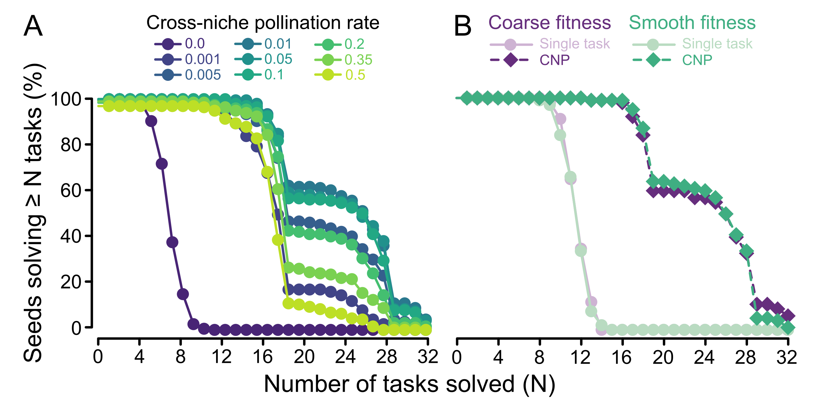
We tested whether explicitly smoothing the fitness function by other means could replicate the benefit of applying a moderate CNP rate. The binary success/fail signal was therefore replaced with a graded one, scaling the interaction probability linearly with how far a program’s outputs fell from the correct values on the validation inputs (see for the exact formulation). We ran a control setup where each of the tasks was evolved in complete isolation (the ‘Single Task’ setup). In these runs, we kept the exact same overall compute budget and \(512 \times 1024\) grid structure as the CNP system. Consequently, the population dedicated to a single task (\(524,288\) programs) was 32 times larger than a single \(128 \times 128\) niche in the CNP setup. Despite this 32-fold population advantage per task, these isolated populations failed to progress, solving at most 15 of the simplest tasks out of the total set (Fig. 4B). In contrast, the CNP system, which partitioned the same global population across 32 smaller, interconnected niches, drastically outperformed them. This difference reveals a dynamic related to the objective paradox within algorithmic evolution—the phenomenon where directly optimizing for a complex target objective often prevents its discovery, whereas optimizing for intermediate stepping stones succeeds. Assembling complex logic (such as nested accumulation loops for polynomial evaluation) requires distinct, discontinuous algorithmic modules, and the spatial structure of the CNP system allowed these modules to be combined across niches, whereas they would be unlikely to arise in a single-task population.
3 Discussion↩︎
In this paper, we examined the co-evolution of self-replication and problem solving within a digital primordial soup (Fig. 1). Building upon [15], we found that self-replication and task solutions both reliably emerged from random noise. Unlike traditional evolutionary systems where reproduction is a fixed background rule, here replication and problem-solving
mechanisms co-evolved and shared a 32-byte memory. (It should be noted, though, that unlike the case with the origins of life on Earth, our programs were initialized with elements that have predefined computational semantics.) The transition from
pre-evolutionary stochasticity to Darwinian evolution was shaped by the pressure exerted by the tasks. This computational pressure drives a feedback loop where the demand to solve tasks actively reshapes the machinery of heredity itself, steering
populations away from naive copying mechanisms that monopolize the tape and accelerating the emergence of more compact, robust replication architectures, such as LDIR and LDD loops, that leave room for task-solving code (Fig. 2). In this way, the demands placed on what a program computes feed back onto the architecture of how it reproduces. Similarly, metabolic constraints encouraged the evolution of programs that halt at appropriate times
to optimize their execution budget. Notably, these halting behaviors sometimes evolved to function in a conditional manner, allowing programs to distinguish between validation and interaction executions (Fig. 3).
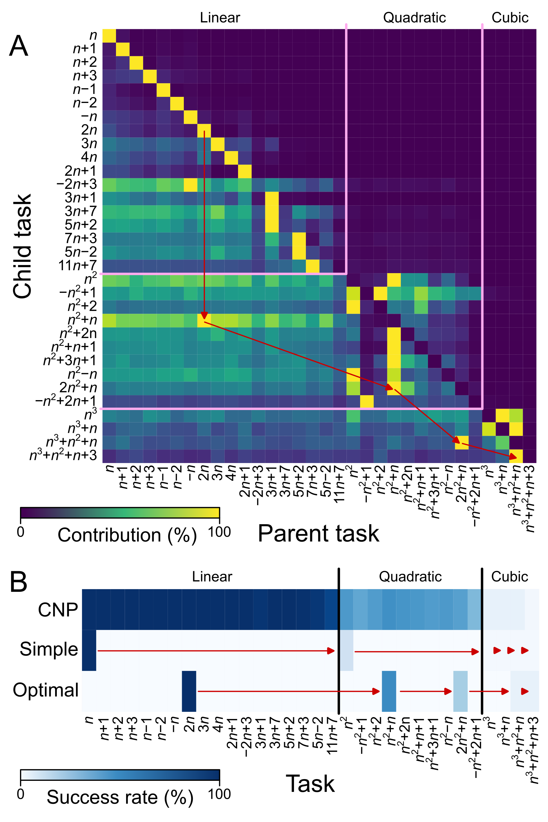
We leveraged spatially structured task niches as a framework to investigate the learning capabilities of this co-evolutionary system. In our experiments, populations working in isolation consistently failed to solve non-trivial polynomials. This failure demonstrates that direct optimization toward a difficult target is fundamentally insufficient in this landscape. Instead, partitioning the population into separate niches connected by sparse pollination allowed the system to self-organize an evolutionary curriculum, where simpler tasks served as essential stepping stones to seed solutions for more complex ones (Fig. 4). When we compared this self-organized process to a hand-designed curriculum of steadily increasing complexity, the hand-designed path failed. This contrast highlights that the spatial niche structure acts as a decentralized engine for discovering evolutionary pathways (Fig. 5).
One limitation of this study is that we did not systematically investigate the interaction dynamics for the emergence of genetic diversification, such as recombination or symbiogenesis. Our interaction protocol does not preclude genetic mixing, and accidental recombination may have played a role in evolutionary transitions. This contrasts with traditional genetic algorithms where crossover is fixed a priori [26], [43]. However, most of the dominant replicators we manually inspected employed asexual reproduction. Investigating whether programs can spontaneously discover reciprocal genetic exchange remains an important direction for future work.
Another limitation of this study was that the tasks used (calculating polynomials) were, despite Z80 lacking a multiplication instruction, relatively simple and drawn from the same class. While the use of simple tasks and restricted domains is in line with previous work on algorithmic evolution in ALife [30], [31], follow-up research could explore how tasks and self-replication co-evolve when the tasks and their domains are wider and drawn from a real-world relevant set. Finally, there was a ceiling on the complexity of algorithmic solutions that could be discovered, both due to the hard limit of 32-byte program lengths, and due to the absence of cooperative mechanisms for programs to co-solve tasks. Future research could explore how self-replication and tasks co-evolve when more complex, potentially multi-agent, solutions are possible.
In total, our work demonstrates that mechanisms of inheritance and fitness optimization can co-evolve to shape one another, and supports the perspective that origin-of-life and evolutionary computation research can view evolution not merely as a static search algorithm, but as a dynamic, plastic property of an open-ended learning system.
4 Methods↩︎
4.1 Competence-gated interaction and metabolic constraints↩︎
Interactions between programs are biased by their ability to solve the polynomial task assigned to their niche (Fig. 1C). Before a selected program \(P_1\) is allowed to interact, it
undergoes a validation phase. We place \(P_1\) in the first half of the \(2\ell\)-byte memory and zero the second half, and execute the tape for a maximum budget of \(B=512\) instructions. For this validation run, the Z80 registers are initialized as follows: registers HL, BC, and E, and the program counter PC are set to zero; register
A and the stack pointer are set to 0xFF; and register D is initialized with the task input \(x\). Since the emulated address space is limited to \(2\ell\) bytes and every memory access is taken modulo \(2\ell\), the stack pointer value 0xFF resolves to the last byte of the tape, so stack writes grow backwards from the end of
the memory. The output is read from register E (which, being an 8-bit register, implicitly stores the result modulo \(2^8\)). During the subsequent interaction phase, the register initialization is identical,
except that register D is initialized to zero rather than the task input.
To pass validation, \(P_1\) must satisfy \(\mathtt{E}=f(x) \bmod 2^8\) for three inputs drawn without replacement from \(\{0,\ldots,15\}\), where \(f\) is the polynomial associated with \(P_1\)’s niche. Evaluating a subset of three inputs is sufficient to make accidental successes by incorrect programs highly improbable. Programs that pass receive an elevated interaction probability \(p_{\mathrm{succ}}=1.0\); programs that fail keep the baseline probability \(p_{\mathrm{base}}=0.3\).
To simulate metabolic constraints, we discount the interaction probability of validated programs in proportion to the number of execution steps they spend during validation. The interaction probability is \[p(\text{interaction}) = \begin{cases} p_{\mathrm{succ}} - C \dfrac{k}{B} & \text{if validated} \\[6pt] p_{\mathrm{base}} & \text{otherwise} \end{cases}\] where \(k\) is the average number of execution steps taken over the three validation runs, \(B=512\) is the maximum instruction budget, and \(C\) is the metabolic penalty coefficient. The penalty is applied only to validated programs; the probability of a failed program is fixed at \(p_{\mathrm{base}}=0.3\) regardless of its execution cost. Unless otherwise stated we set \(C=0.3\); the sweep reported in Fig. 3 instead varies \(C\) across \([0, 0.7]\).
Validation is distinct from solving a task. Validation gates interaction and is decided on three sampled inputs, whereas we report a task as solved on the basis of the full input range. Concretely, throughout the paper we count a niche as having solved its task when at least \(10\%\) of its programs produce \(f(x) \bmod 2^8\) correctly for every \(x \in \{0,\ldots,15\}\), and not merely for the three validation draws.
4.2 Smooth fitness landscape control↩︎
In control experiments evaluating the impact of a smoothed fitness landscape, we replaced the binary success/fail validation with a graded interaction probability. The probability was scaled linearly with the average numerical distance between the program’s outputs and the target values across the validation inputs: \[\begin{align} \text{penalty} & = 1 - \frac{k C}{512} \\[1ex] \text{avg dist} & = \frac{ \mathop{\raisebox{0.6ex}{\sum\limits_{y \in f(X)}}} \frac{\operatorname{mod}(y,\hat{y})}{128} }{ \lvert X \rvert } \\[1ex] p(\text{interaction}) & = \max\left(0.3, \left( 1 - 0.7 \cdot \text{avg dist}\right) \cdot \text{penalty}\right) \end{align}\] where \(\operatorname{mod}(a, b)\) refers to the distance between \(a\) and \(b\) modulo 256, \(X = \{x_1,x_2,x_3\}\) is the set of inputs for verification, \(y=f(X)\) is the set of target outputs for the polynomial function \(f\), and \(\hat{y}\) is the set of outputs from the program for each input.
4.3 Simulation protocol↩︎
Simulations run for \(T_{\max} = 10^6\) epochs starting from uniformly random bytes. Parameters are summarized in Table 1.
| Program length \(\ell\) | 32 bytes |
| Instruction budget \(B\) | 512 |
| Global grid | \(512 \times 1024\) |
| CNP sub-environments | 32 (each \(128 \times 128\)) |
| Baseline interaction prob.\(p_{\mathrm{base}}\) | 0.3 |
| Success interaction prob.\(p_{\mathrm{succ}}\) | 1.00 |
| Cross-niche pollination \(\pi\) | 0.05 |
| Per-program mutation rate | 1/64 |
| Validation draws | 3 inputs, no replacement |
| Validation domain | \(x \in \{0,\ldots,15\}\) |
| Output modulus | \(2^8\) |
| Max epochs \(T_{\max}\) | \(10^6\) |
| Replicates per condition | 100 |
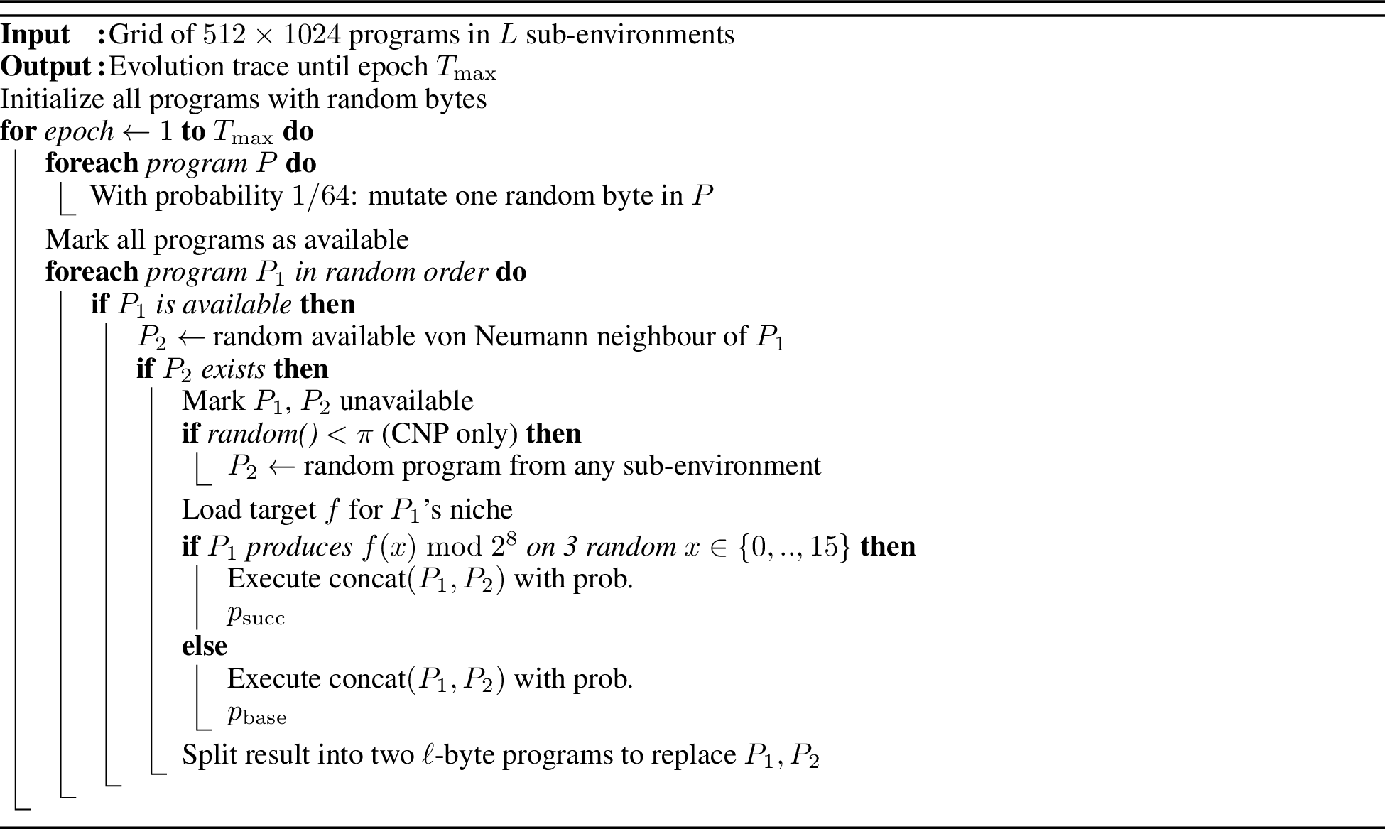
To implement the pairwise interaction loop in Algorithm 6 without overlapping or order bias, candidate pairs are generated each epoch by randomly shuffling all grid positions and drawing a partner for each selected program. Because programs can be drawn more than once across candidate pairings, any pair containing a duplicate program assignment is filtered out before execution to ensure that no cell is evaluated or overwritten more than once per step. Because of this filtering step, the pairing algorithm is stochastic, and a randomly varying number of programs (on average roughly 56% of the population) are selected every step for validation and interaction.
4.4 Replicator population dynamics with and without tasks↩︎
To understand the extent to which imposing task validation influences the underlying methods of replication, we compared replicator population dynamics with and without tasks being applied. We present the results of this investigation in Figs. 2D and 2E. To calculate the population counts, we used a byte-matching search to count known replicators of each type. Specifically, we scanned for the following consecutive
byte sequences corresponding to key instructions for each replicator, which rely on the Z80’s core block-copy registers (HL for source address, DE for destination address, and BC for copy length):
LDIR (
[0xED, 0xB0]): The repeating block-copy instruction. Setting \(\mathtt{HL}\) to the start of parent \(P_1\), \(\mathtt{DE}\) to the start of partner \(P_2\), and \(\mathtt{BC}\) to 32 copies the entire program automatically in a single step as pointers increment and \(\mathtt{BC}\) decrements to zero.LDDR (
[0xED, 0xB8]): A close relative of LDIR that decrements the pointers instead of incrementing.LDI (
[0xED, 0xA0]): A non-repeating variant of LDIR that increments pointers and decrements \(\mathtt{BC}\) but does not loop automatically.LDD (
[0xED, 0xA8]): A non-repeating variant that decrements pointers and decrements \(\mathtt{BC}\) but does not loop automatically, requiring an explicit external loop to achieve replication.LoadPush families: Rely on a sequence of paired load and stack-push instructions (e.g., loading bytes into a register and pushing them onto the stack). We tracked four variants based on the registers used:
LoadPush (BC):
[0x01, 0xC5, 0x01, 0xC5]LoadPush (DE):
[0x11, 0xD5, 0x11, 0xD5]LoadPush (HL):
[0x21, 0xE5, 0x21, 0xE5]LoadPush (HL_2):
[0xE5, 0x2A, 0xE5, 0x2A]
We identified these key instructions by manually inspecting our runs and looking at execution traces to see what elements of tape were responsible for replication.
A tape was counted if it contained the target sequence at least once. Formally, for a set of tapes \(T\) and a byte pattern \(p\), the population count \(C_{p}\) is given by:
\[C_{p} = \sum_{t \in T} \mathbb{I}(p \subseteq t)\]
where \(\mathbb{I}\) is the indicator function returning 1 if the pattern \(p\) exists as a contiguous subsequence in tape \(t\), and 0 otherwise. The overall counts for the LDIR and LoadPush families were calculated as the sum of these unique tape counts across their respective variants (\(v\)):
\[C_{\text{LDIR}} = \sum_{v \in \{\text{LDIR, LDDR, LDI, LDD}\}} C_{v}\]
\[C_{\text{LoadPush}} = \sum_{v \in \{\text{BC, DE, HL, HL\_2}\}} C_{\text{LoadPush}(v)}\]
We note that this is not an exhaustive list of possible replicators, and likewise not a perfect search for replicators of this type (for instance, a NO-OP instruction could easily exist between the bytes of an LDIR, and it would functionally behave the same, but wouldn’t be picked up by our search). However, in all cases the sum of all replicator families closely matches the total tape population size, so we expect the figures to be a sufficiently faithful count of the majority of replicator tapes.
To generate Fig. 2D, we initialized 100 runs with different random seeds for each of the two experiment types: with task validation applied, and without it. In both settings, the number of niches and the number of tapes remained the same. For the experiments without task validation, we simply skipped the validation step (including penalizing execution length), and every tape proceeds to interaction. We then computed the average population counts of the replicators across these 100 seeds every 1000 steps.
To generate Fig. 2E, we repeated the same experiment as for Fig. 2D, but in this case we customized the Z80 emulator we were using to turn the key instruction byte pairs for all the LDIR-family replicators except LDD into the equivalent of NO-OPs. In other words, we deactivated all LDIR-family instructions except LDD. We then computed population counts the same way as for Fig. 2D.
In both cases, Tasks Solved is defined as the number of niches where \(\geq 10\%\) of the tapes successfully solve the task across the entire input domain.
4.5 Replicator robustness to mutations↩︎
To compare how well the three replicator architectures tolerate mutation (Fig. 2F), we measured whether each one retains its ability to copy itself after a number of mutation events. We seeded each test with a
canonical replicator of the relevant type. The LDIR replicator was the four bytes [0x1E, 0x20, 0xED, 0xB0], which set register E to 32 and then executed the LDIR instruction while relying on the default initialization
\(\mathtt{HL}=\mathtt{BC}=0\), followed by 28 uniformly random bytes drawn independently in each trial to fill the tape to 32 bytes. Because the LDIR instruction copies all 32 bytes verbatim, the content of
this trailing region does not affect replication and is reproduced faithfully along with the functional prefix. The LDD replicator was the eleven bytes [0x2E, 0x1F, 0x1E, 0x3F, 0x0E, 0x20, 0xED, 0xA8, 0x28, 0xFC, 0x76], which initialize
registers L, E, and C, run the LDD instruction inside a loop closed by a conditional relative jump, and end with a HALT, again padded with zeros to 32 bytes. The Load-Push replicator was the
byte pair [0x01, 0xC5], a load followed by a stack push, repeated sixteen times to fill the 32 byte tape.
Each robustness trial consisted of \(n\) successive mutation and replication cycles, with \(n \in \{1, 4, 8\}\). In every cycle we first mutated the current genome by selecting one byte position uniformly at random among its 32 positions and replacing it with a uniformly random byte in \(\{0,\ldots,255\}\), exactly as in the simulation’s mutation operator. Because each position is drawn afresh, the replacement may coincide with the original byte and the same position may be selected in more than one cycle. We then placed the mutated genome in the first half of a \(2\ell\)-byte tape, set the second half to zeros, and executed the tape for up to \(B=512\) instructions under the same register initialization used during interaction. The first half of the resulting tape, which holds the program itself, became the genome carried into the next cycle. We classified a trial as a success when, on the final cycle, the second half of the executed tape, which had started as zeros, was byte-for-byte identical to the first half, indicating that the mutated program had copied all 32 of its bytes into the empty partner.
For each replicator type and each value of \(n\) we ran 100 independent trials and report the fraction that succeeded, with error bars given by 95% Wilson score intervals. Pairwise differences between replicator types at each mutation level were assessed with one-sided two-proportion \(Z\)-tests using Bonferroni correction across the comparisons.
4.6 Metabolic penalty sweep and halting behavior↩︎
To probe how the metabolic constraint shapes the evolved programs (Fig. 3), we swept the penalty coefficient \(C\) across the eight values \(0.0, 0.1, \ldots, 0.7\). For each value we ran 100 independent simulations, giving \(N=800\) runs in total. Every run used the standard configuration of 32 niches with cross-niche pollination for \(10^6\) epochs. All quantities below were measured on the final state of each grid.
For the average execution length (Fig. 3A), we performed a single validation run for every program in the final grid. We set register D to one input \(x\) sampled
uniformly from \(\{0,\ldots,15\}\) for each program, placed the program in the first half of a \(2\ell\)-byte tape with the second half set to zeros, and executed for up to \(B=512\) instructions, recording the number of instructions executed, which equals \(B\) when the program never halts. This per-program count is the validation execution step quantity \(k\) plotted in Fig. 3A. We averaged this count over all programs in the grid to obtain one value per run. The 100 values at each coefficient are shown as box plots, with median,
interquartile range, and whiskers at \(1.5\times\) the interquartile range, and the individual runs overlaid. The association between \(C\) and the per-run average was quantified with
Spearman’s rank correlation over the \(N=800\) runs.
For the halting behavior (Fig. 3B), we restricted attention to the programs that produced the correct output on a single sampled input, that is, the programs whose validation run above returned \(\mathtt{E}=f(x) \bmod 2^8\). Each such program was executed in two environments that differ only in the value of register D, in both cases with the partner half of the tape set to zeros and a budget of \(B=512\) instructions. In the validation environment register D held the sampled input \(x\); in the interaction environment register D was zero, as it is during a
normal interaction. In each environment we recorded whether the program reached a HALT within the budget or instead ran to the budget without halting, and we assigned the program to one of four mutually exclusive categories: it halted in both
environments (Both), only in the validation environment (Validation), only in the interaction environment (Interaction), or in neither (Neither).
Within each run we normalized these counts to percentages of the filtered set of programs, so that the four categories sum to \(100\%\) and every run carries equal weight regardless of how many programs it contributed. Each subplot of Fig. 3B corresponds to one category: the bar height is the median percentage across the runs at that coefficient, and the error bars are the \(95\%\) confidence interval of the median, obtained by non-parametric bootstrapping with 1000 resamples and drawing the lower and upper caps at the 2.5th and 97.5th percentiles of the resulting distribution of medians. The Validation category corresponds to the conditional halting described in the main text, in which a program halts during validation but skips the halt during interaction. Its association with \(C\) was quantified with Spearman’s rank correlation over the \(N=800\) runs.
4.7 Computation of the ancestor contribution matrix↩︎
To trace the phylogenetic history of the emergent programs and uncover the evolutionary pathways (Fig. 5A), we tracked the niche of origin for all lineages throughout the simulation. At initialization (epoch 0), every program in the grid was labeled with an ancestor niche ID equal to its own niche \(j \in \{0, \dots, L-1\}\), where \(L = 32\) is the total number of niches. This label was then carried through interactions to record the most recent solved niche from which each lineage received material. When a validated program \(P_1\) interacted with a neighbor \(P_2\) within its own niche, the two programs written back in their place both took on \(P_1\)’s ancestor niche ID. When instead a cross-niche pollination event paired \(P_1\) with a partner \(P_2\) drawn from a different niche, the program written back in place of \(P_2\) adopted the current niche index of \(P_1\) as its ancestor niche ID, but only when \(P_1\)’s niche had already been marked as having solved its task. A program’s ancestor niche ID therefore identifies the most recent solved niche from which its active replicating lineage received material, defaulting to its niche of origin.
We defined a niche \(i\) as having successfully solved its assigned task \(i\) at the earliest epoch \(t\) where the fraction of programs in the niche solving the task across the entire input domain (\(16\) distinct inputs) was at least \(10\%\) (corresponding to \(\ge 1,639\) programs in a \(128 \times 128\) subgrid). At this exact epoch, we recorded a snapshot of the ancestor niche IDs of all programs in niche \(i\). Specifically, we computed a raw ancestor contribution vector for niche \(i\), where the \(j\)-th component \(A_{i, j}\) represents the number of programs in niche \(i\) belonging to lineages that originated in niche \(j\):
To aggregate this data across multiple independent runs, we performed the following normalization steps. First, for each simulation run \(g \in \{1, \dots, G\}\) (where \(G = 2000\) is the total number of random seeds), we normalized the raw counts to obtain the relative contribution of each source niche to the solution of task \(i\): \[N^{(g)}_{i, j} = \frac{A^{(g)}_{i, j}}{\sum_{k} A^{(g)}_{i, k}}\] conditioned on the task being solved in that run (\(\sum_{k} A^{(g)}_{i, k} > 0\)), and setting \(N^{(g)}_{i, j} = 0\) otherwise. Next, we computed the conditional average of these relative contributions across all runs where task \(i\) was successfully solved: \[V_{i, j} = \frac{\sum_{g=1}^{G} N^{(g)}_{i, j}}{\sum_{g=1}^{G} \mathbb{I}\left(\sum_{k} A^{(g)}_{i, k} > 0\right)}\] The matrix \(V\) represents the average proportion of the population in niche \(i\) originating from niche \(j\) at the moment the task was solved, conditioned on task \(i\) being solved. Finally, to construct the unified heatmap (Fig. 5A), we applied a row-wise min-max normalization to highlight the relative significance of different source niches for each target task, independent of the absolute magnitude of contributions: \[W_{i, j} = \frac{V_{i, j} - \min_{k} V_{i, k}}{\max_{k} V_{i, k} - \min_{k} V_{i, k}}\] where \(W_{i, j} \in [0, 1]\) is the normalized relative contribution of source task \(j\) to target task \(i\).
4.8 Curriculum learning↩︎
To investigate curriculum learning, we maintain the same spatial topology as the CNP configuration: a population of \(N_p = 524,288\) programs distributed across a grid divided into \(L = 32\) separate niches (subgrids of \(128 \times 128\) programs), with local neighborhood pairing and a global cross-niche pollination rate of \(\pi = 0.05\). However, instead of each niche evaluating programs on a distinct static task from the task library, all \(L\) niches in the population are evaluated on the same target task \(T_i\) at any given epoch. This target task is updated dynamically as the population traverses a linear curriculum sequence \(\mathcal{C} = \langle t_1, t_2, \dots, t_K \rangle\), which is defined as either: \(\mathcal{C}_{\text{optimal}} = \langle 2n, \;n^2+n, \;2n^2+n, \;n^3+n^2+n, \;n^3+n^2+n+3 \rangle\), or \(\mathcal{C}_{\text{simple}} = \langle n, \;n^2, \;n^3, \;n^3+n, \;n^3+n^2+n, \;n^3+n^2+n+3 \rangle\).
To enable evolutionary scaffolding and prevent the loss of capabilities acquired in the previous step, the interaction probability is:
\[p(\text{interaction}) = \begin{cases} 1.0-\frac{kC}{512} & \text{ if T_i validated} \\ 0.65-\frac{kC}{512} & \text{ else if T_{i-1} validated} \\ 0.3 & \text{ otherwise} \end{cases}\]
where \(T_i\) is the active task and \(T_{i-1}\) is the immediately preceding task in the curriculum (with \(T_0\) defaulting to not validated), \(k\) is the average number of execution steps taken over the three validation runs, \(B=512\) is the maximum instruction budget, and \(C\) is the metabolic penalty coefficient.
The active curriculum task advances globally from \(T_i\) to \(T_{i+1}\) (setting the target task for all niches to \(T_{i+1}\)) at the end of any logging batch if at least one program in any of the niches successfully solves the active task in its complete domain. The total computational budget is kept identical to the CNP benchmark runs.
Author Contributions↩︎
F.C., E.N., E.R., and B.R. designed research; F.C., E.N., E.R., and S.B. performed research; F.C., E.N., and A.B. analyzed data; and F.C., E.N., E.R., S.B., A.B., M.E., R.S., C.K., B.L., J.M., B.A.A., and B.R. wrote the paper.