Interference and Retention in Continual Learning
July 10, 2026
Abstract
Continual learning commonly relies on post-hoc mechanisms such as replay, elastic regularization, or distillation. This work argues that forgetting should instead be modeled directly as interference between tasks. In the frozen-feature regime, forgetting from learning a new task is exactly the interference energy induced on the old task. In deep networks, the same quantity is recovered through path-averaged curvature with minimal additional forward passes.
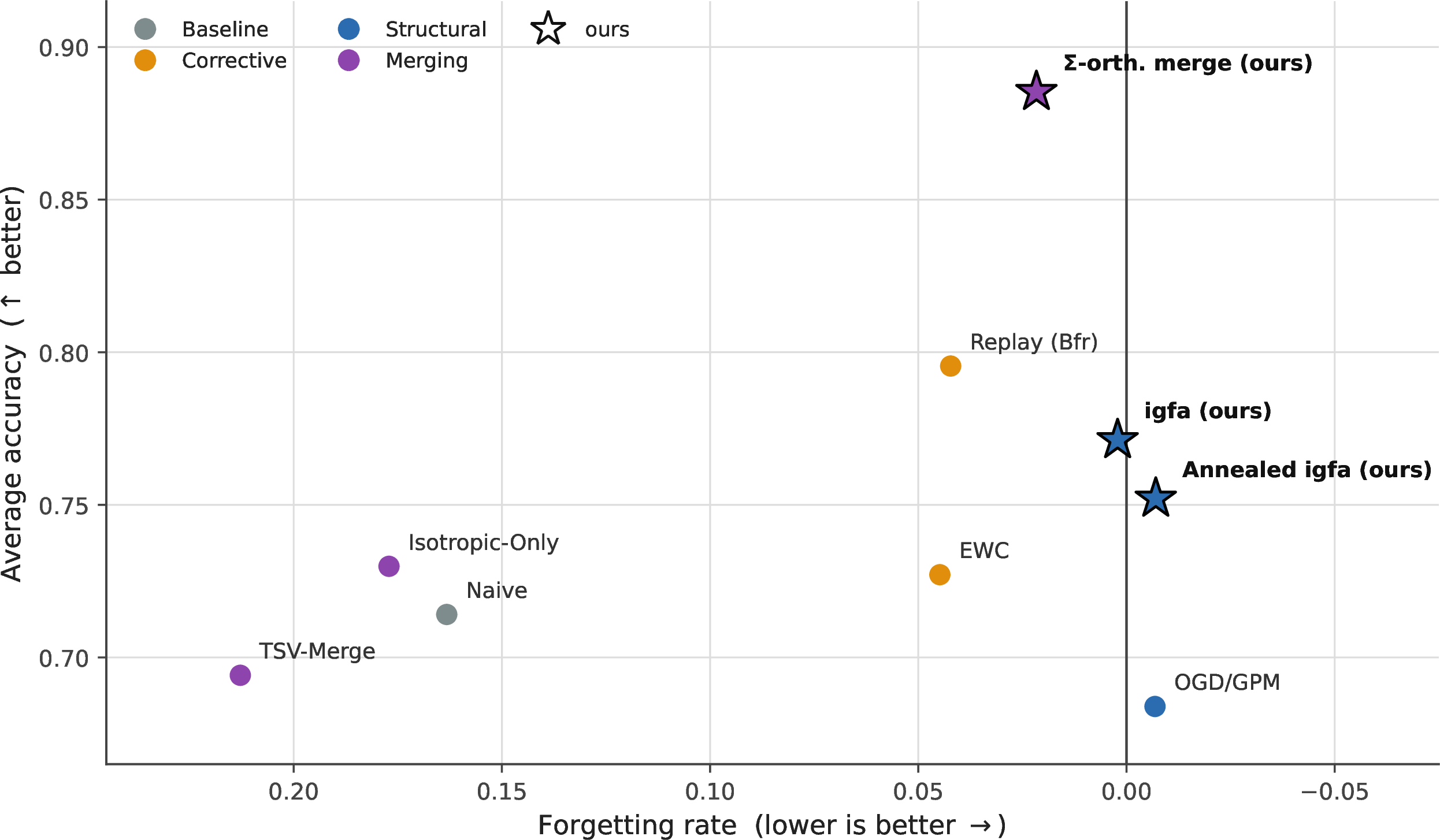
When task supports are disjoint, forgetting can be eliminated structurally and when task supports overlap in conflicting directions, a non-zero distortion floor is unavoidable. The same geometry optimally merges models through task-aware orthogonalization. From this analysis we derive Interference-Gated Functional Allocation (igfa), a replay-free, Fisher-free method that shares directions when tasks align and protects them when they conflict. Across benchmarks, igfa achieves lossless retention when tasks are structurally separable and moves unavoidable cost from irreversible forgetting into deferred but recoverable plasticity when they are not. It matches the strongest replay-free structural baselines on dissimilar-task streams and improves on unconditional projection when similarity makes transfer worth preserving.
Keywords: continual learning; catastrophic forgetting; model merging; neural tangent kernel; gradient projection; rate–distortion; representation geometry
1 Introduction↩︎
A model trained sequentially on task \(B\) after task \(A\) often degrades on task \(A\), a phenomenon known as catastrophic forgetting. Networks trained by stochastic gradient descent (SGD) or its variants update from the current minibatch alone (or a smoothed average of a short window of minibatches); the update is therefore oblivious to past knowledge. This obliviousness is desirable when the training data are i.i.d., but harmful once the training distribution shifts over time in the continual setting. Standard approaches such as replay [1]–[3], elastic weight consolidation [4], [5], and distillation [6] mostly repair forgetting after interference has already occurred. What is still missing is a predictive account of when interference is avoidable, when it is inevitable, and what structure an update must satisfy to retain old behavior without sacrificing useful transfer.
This work focuses on the linear-on-features regime in which a frozen feature extractor \(\phi(x)\) is paired with a trainable linear head, covering the common frozen-backbone and parameter-efficient fine-tuning (PEFT) settings and the first-order neural tangent [7] approximation of a fully trained network. The forgetting of an earlier task \(A\) after an update \(\Delta\) caused by learning task \(B\) is exactly the interference energy \(\tfrac12\,\Delta^\top\Sigma_A\Delta\), where \(\Sigma_A\;= \mathbb{E}_{x \sim D_A}\left[\phi(x)\phi(x)^\top\right]\) denotes the feature second moment of task \(A\), measuring which feature directions are active for that task. The same geometry predicts per-task forgetting accurately and extends approximately to deeper networks with feature drift.
The paper makes three contributions.
Interference functional and removability. We derive an exact interference functional for forgetting. In the frozen-feature regime, forgetting is exactly the old task’s interference energy under the new update, which yields a clean criterion for when retention is lossless and when a distortion floor is unavoidable. The geometry of \(\Sigma_A\) penalizes only components in its active subspace, while updates in \(\ker \Sigma_A\) leave task \(A\)’s loss unchanged. This yields a structural criterion for lossless retention: interference is removable for disjoint task supports (reducing to ordinary orthogonality in isotropic geometry), whereas overlapping supports imply a non-zero distortion floor. The same quantity also admits an information-theoretic interpretation through the task-inference problem.
Optimal merging as \(\Sigma\)-orthogonalization. We show that optimal merging is task-aware orthogonalization. This unifies offline model merging and online continual learning as batch and incremental solutions for minimizing the same interference objective. Section 3.4 shows that post-merge loss decomposes into task-wise fit and cross-task interference. Minimizing this objective requires mutual \(\Sigma\)-orthogonality of the task vectors, yielding the optimality condition for model merging.
Interference-Gated Functional Allocation. We introduce igfa, a replay-free structural controller. The method shares capacity when tasks align, protects it when they conflict, and retains only a low-rank subspace summary. Section 4 introduces igfa, an online method motivated by the same functional (Fig. 2).
![Figure 2: The task-induced geometry in feature space motivates either full sharing, full separation, or selective parameter sharing. Left (Disjoint). When two tasks excite orthogonal feature subspaces, the update \Delta is composed of a component \Delta_\parallel\in\mathop{\mathrm{range}}\Sigma_A between the iso-loss contours that incurs forgetting and \Delta_\perp\in\ker\Sigma_A along the iso-loss contours where allocation is interference-free. Centre (Overlapping). When the supports share an active direction, no update for B can avoid \mathop{\mathrm{range}}\Sigma_A and a distortion floor is unavoidable. Right. The same functional yields three update rules. Naive descent incurs the full interference (distorts old knowledge); orthogonal projection (ogd/gpm [8], [9]) removes all overlap (no forgetting, but no transfer and capacity exhaustion); igfa applies a signed gate—sharing aligned directions and orthogonalizing conflicting ones—balancing retention and transfer while carrying only the occupied subspace as state.](/article/2607.09202/figures/Subspace_Interference_and_Forgetting_Geometry.png "fig:")
The experiments in Section 5 are designed to test the theory directly, including lossless allocation on disjoint supports, the relocation of unavoidable cost from forgetting into deferred plasticity, the similarity threshold at \(s^{\ast}\approx0.26\), and the onset of a capacity floor once the cumulative occupied rank reaches the feature dimension, \(T\,r\approx d\) (with \(T\) the number of tasks in the stream, \(r\) the rank of the feature subspace each task occupies, and \(d\) the feature dimension). In the frozen-feature Split-Digits setting, igfa matches the strongest replay-free and Fisher-free baseline at about \(0.98\) accuracy with near-zero forgetting while using no replay buffer. Extensions to full-network training, large-scale overlays, and direct comparison with replay at scale are discussed in Section 6, with the supporting experiments detailed in the Supporting Information.
2 Related work↩︎
2.0.0.1 Corrective continual learning.
Replay [1]–[3], regularization [4], [5], and distillation [6] remain the main corrective approaches to continual learning. They do not explicitly model interference through task geometry however, while the herein derived interference functional predicts the collision of the task updates and identifies when it can be removed before occuring. Replay can be viewed as a stochastic Monte-Carlo estimator of the same task second-moment \(\Sigma_t\) that we estimate sample-free via a low-rank subspace.
2.0.0.2 Geometry- and gradient-based methods.
A related line of work controls the update direction itself. Orthogonal Gradient Descent [8], Gradient Projection Memory [9], and Orthogonal Weight Modification [10] project updates away from subspaces associated with previous tasks. Under a fixed-feature map, this corresponds to enforcing \(\Delta\in\ker\Sigma_A\). PCGrad-style methods [11] resolve conflicts through pairwise gradient comparisons rather than explicit task-subspace protection. Recent work also studies closely related regimes: Geodesic-Aligned Gradient Projection [12] addresses feature drift during sequential learning, and MINGLE [13] uses a null-space criterion to gate low-rank experts during test-time merging. Relative to these approaches, the present framework derives the projection condition from an exact forgetting functional, replaces unconditional projection with a similarity-gated share-or-orthogonalize rule, and uses the same functional to characterize both merging and the distortion floor. NTK-based analyses [14], [15] likewise relate forgetting to overlap in representation space, but do not develop the \(\Sigma\)-orthogonality criterion or the associated transfer gate.
2.0.0.3 The averaged Jacobian as a shared object with interpretability.
A convergent notion of geometry appears in mechanistic interpretability. The Jacobian lens of Gurnee, Lindsey, et al. [16] characterizes a residual-stream activation by its context-averaged forward Jacobian \(J_\ell=\mathbb{E}[\partial h_{\mathrm{final}}/ \partial h_\ell]\) composed with the unembedding, and identifies the low-rank span of its active readout directions—the “J-space”—as the subspace of verbalizable representations, limited in capacity and competitively occupied, a language-model global workspace. Our interference geometry is the learning-dynamics counterpart of the same move: where the J-lens averages the forward activation\(\to\)output Jacobian, we average the Gauss–Newton curvature \(\Sigma_A=\mathbb{E}[J_wJ_w^\top]\) (Sec. 3.3), and both replace a single-point Jacobian with a distribution-averaged one for the same stated reason—to isolate an architecture-level invariant from context-specific use. The two induce the same partition of representation space: their causally load-bearing J-space plays the role of our \(\mathop{\mathrm{range}}\Sigma_A\) (perturbations there change outputs and incur forgetting), and the inert complement that their coordinate-patching “leaves unchanged” is our \(\ker\Sigma_A\) (free directions). Read this way, our interference energy and distortion floor supply a quantitative model of workspace competition and our occupied-rank capacity knee a rate–distortion account of its limited capacity; conversely, the released lens is a ready estimator of the averaged-Jacobian subspace our method tracks at scale. We make the connection testable in Sec. 6.
2.0.0.4 Model merging and task arithmetic.
In a parallel line of literature, independently fine-tuned are combined into a single model that retains useful knowledge from each task through arithmetic on weight-space task vectors [17], [18]. These methods usually operate in Euclidean parameter space, whereas the present analysis identifies the task-dependent metric induced by \(\Sigma_t\) as the relevant geometry. Under this metric, optimal merging becomes mutual \(\Sigma\)-orthogonalization, with ordinary weight-space orthogonality recovered only when \(\Sigma_t\propto I\). Task Singular Vectors [19] promotes orthogonality by whitening singular directions of task vectors; by contrast, isotropic merging [20] shows that shared-subspace isotropy can outperform strict orthogonalization. WUDI-Merging [21] is particularly close in spirit because it links task vectors to input subspaces and minimizes interference without data; the key difference in our work is that the metric and residual are derived from an exact forgetting functional rather than an approximate subspace argument. Tangent-space continual merging [22] also operates in a first-order regime, but with similar trade-offs between scalability and functional specificity. The common perspective adopted here is that the same interference functional governs both offline merging and online continual allocation.
2.0.0.5 Scenarios, scale, and plasticity.
The standard task-, domain-, and class-incremental taxonomy [23] distinguishes whether task identity is given or must be inferred. In this context, the distortion floor developed later provides a quantitative link between support overlap and task inference. Related empirical and analytical work has examined the effects of scale and pretraining [24], frozen-backbone prompt and adapter methods [25]–[27], which learn prompt pools with input-conditioned selection under a class-incremental protocol and provide strong empirical accuracy without structural retention guarantees (differentiated in Sec. 5.6), forgetting in linear models [28], plasticity loss [29], and convergence or task ordering in continual linear classification [30], [31].
3 Preliminaries: the interference functional↩︎
This section specifies the setting and assumptions (Sec. 3.1), derives the interference functional and the removability dichotomy (Sec. 3.2), generalizes the identity beyond frozen features (Sec. 3.3), and derives the optimal merge together with the distortion floor (Sec. 3.4).
3.1 Setting and assumptions↩︎
Let \(\phi:\mathcal{X}\to\mathbb{R}^d\) be a fixed feature map and \(w\in\mathbb{R}^d\) a trainable linear head with prediction \(\hat{y}=w^\top\phi(x)\). For task \(t\), let \(\Sigma_t=\mathbb{E}_{x\sim\mathcal{D}_t}[\phi(x)\phi(x)^\top]\succeq0\) denote the feature second moment, and let \(w_t^\ast\) be a realizable optimum. The per-task excess loss is \[L_t(w)=\tfrac12\,(w-w_t^\ast)^\top\Sigma_t\,(w-w_t^\ast)\;\ge 0. \label{eq:excess}\tag{1}\] Under squared loss, this coincides with the excess population risk. We write the target as \(y=\phi(x)^\top w_t^\ast+\varepsilon\) to separate the predictable linear component from the irreducible residual variation. With \(y=\phi(x)^\top w_t^\ast+\varepsilon\), \(\mathbb{E}[\varepsilon]=0\), and \(\varepsilon\!\perp\!\phi(x)\), the squared risk satisfies \(\mathbb{E}[(\hat{y}-y)^2]/2=L_t(w)+\tfrac12 \mathbb{E}[\varepsilon^2]\), so all subsequent loss differences depend only on \(L_t(w)\).
Three assumptions define this regime: (A1) frozen features—\(\phi\) is fixed during training, exact for frozen-backbone and PEFT settings and the first-order NTK [7] model of end-to-end training, so full-network claims are first-order and are tested in Sec. 5.4; (A2) realizability—each \(w_t^\ast\) attains zero excess loss, so mis-specification adds only a task-constant and leaves the interference terms untouched; and (A3) the quadratic regime—training minimizes Eq. 1 by (projected) gradient descent, so motion is confined to the excited subspace while directions in \(\ker\Sigma_t\) leave \(L_t\) unchanged.
3.2 The functional and the removability dichotomy↩︎
Train task \(A\) from a base point \(w_0\) to convergence. Under A3, gradient descent moves only in \(\mathop{\mathrm{range}}\Sigma_A\), so the converged solution \(w_A\) satisfies \(L_A(w_A)=0\) and equals \(w_A^\ast\) up to an arbitrary component in \(\ker\Sigma_A\). For loss differences we therefore take \(w_A=w_A^\ast\). Now train task \(B\), reaching \(w_B\), and define \(\Delta=w_B-w_A^\ast\).
Theorem 1 (Forgetting is interference energy). Under A1–A3, the forgetting of task \(A\) caused by learning \(B\) is \[\Delta L_A=L_A(w_B)-L_A(w_A^\ast)=\tfrac12\,\Delta^\top\Sigma_A\,\Delta, \qquad \Delta=w_B-w_A^\ast. \label{eq:functional}\tag{2}\]
Proof. Since \(L_A(w_A^\ast)=0\) by A2, substituting \(w_B=w_A^\ast+\Delta\) into Eq. 1 yields \(L_A(w_B)=\tfrac12\Delta^\top\Sigma_A\Delta\). No approximation is involved; the only essential assumption is that \(\phi\) remains fixed, so \(\Sigma_A\) is unchanged before and after learning \(B\). ◻
Decompose the update as \(\Delta=\Delta_\parallel+\Delta_\perp\), with \(\Delta_\perp\in\ker\Sigma_A\) and \(\Delta_\parallel\in\mathop{\mathrm{range}}\Sigma_A\). Then \(\Delta L_A= \tfrac12\Delta_\parallel^\top\Sigma_A\Delta_\parallel\), so only the component of the update lying in task \(A\)’s active subspace contributes to forgetting (Fig. 2, left).
Corollary 1 (Removability dichotomy). An update is lossless for \(A\) if and only if \(\Delta\in\ker\Sigma_A\). Consequently there exists a way to learn \(B\) with zero forgetting of \(A\) if \(w_B^\ast\) is reachable through \(\ker\Sigma_A\), i.e. if \(w_B^\ast-w_A^\ast\in\ker\Sigma_A\). Even when this fails, \(L_B\) can still be strictly reduced without forgetting whenever \(w_B^\ast-w_A^\ast\) has a non-zero component in \(\ker\Sigma_A\cap\mathop{\mathrm{range}}\Sigma_B\). If \(\mathop{\mathrm{range}}\Sigma_A\) and \(\mathop{\mathrm{range}}\Sigma_B\) share an active direction on which \(w_A^\ast\) and \(w_B^\ast\) disagree, then no lossless update reaches \(w_B^\ast\), and a positive floor remains (Theorem 5).
Proof. Since \(\Sigma_A\succeq0\), \(\Delta^\top\Sigma_A\Delta=0\Leftrightarrow\Sigma_A^{1/2}\Delta=0 \Leftrightarrow\Delta\in\ker\Sigma_A\). Projected gradient descent on \(L_B\) restricted to \(w_A^\ast+\ker\Sigma_A\) converges to the minimizer on that affine set. It reaches \(w_B^\ast\) if \(w_B^\ast-w_A^\ast\in\ker\Sigma_A\), and it strictly reduces \(L_B\) whenever the projection of \(-\nabla L_B(w_A^\ast)\) onto \(\ker\Sigma_A\) is non-zero, equivalently whenever \(\Sigma_B(w_B^\ast-w_A^\ast)\) has a non-zero component in \(\ker\Sigma_A\). In the disjoint-support case, \(\mathop{\mathrm{range}}\Sigma_B\subseteq\ker\Sigma_A\), so the entire update is lossless. ◻
Here, “task support” refers to the column space \(\mathop{\mathrm{range}}\Sigma_t\), that is, the subspace of feature directions activated by task \(t\). Disjoint supports therefore mean orthogonal feature subspaces, not disjoint label sets.
3.2.0.1 Relation to standard continual-learning metrics.
Under squared loss the per-task term \(\Delta L_A=\tfrac12\Delta^\top\Sigma_A\Delta\) is exactly the per-task summand of the Forgetting Measure and the negative of Backward Transfer; positive backward transfer is simply \(\Delta L_A<0\), which the signed gate permits and unconditional projection forbids. The distortion floor (Sec. 3.4) is then a lower bound on the average Forgetting Measure achievable by any single-head method, set by task confusability (Sec. 9). The geometry thus explains the benchmark metrics and bounds them.
3.3 The architecture-general identity↩︎
Theorem 1 assumes frozen features. In end-to-end training, feature drift degrades the frozen-curvature prediction, especially in deeper networks and at larger step sizes. The natural generalization is to replace \(\Sigma_A\) by the curvature of \(L_A\) averaged along the displacement from \(w_A\) to \(w_B\).
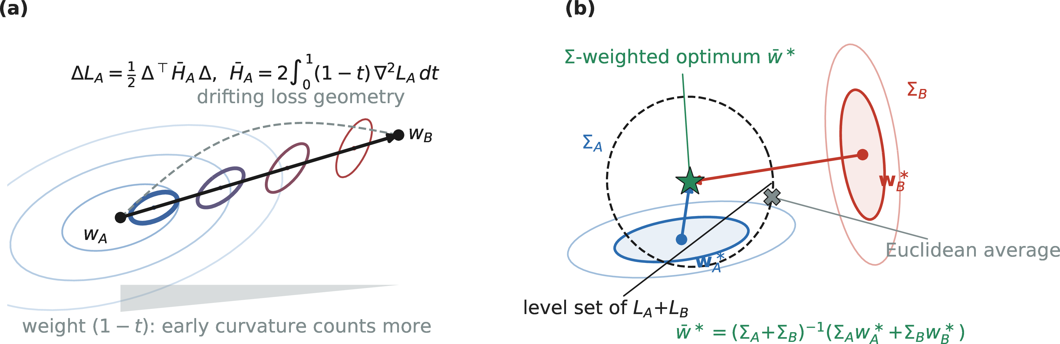
Theorem 2 (Architecture-general forgetting identity). Let \(L_A\) be any twice-differentiable task-\(A\) loss, and let training on \(B\) move the parameters from \(w_A\) to \(w_B\). Writing \(\Delta=w_B-w_A\), \[\Delta L_A=\nabla L_A(w_A)^\top\Delta+\tfrac12\,\Delta^\top \bar H_A\,\Delta, \qquad \bar H_A=2\!\int_0^1(1-t)\,\nabla^2 L_A(w_A+t\Delta)\,dt, \label{eq:general}\tag{3}\] where \(\bar H_A\) is the Hessian of \(L_A\) averaged along the segment \(w_A\!\to\!w_B\). If \(w_A\) is a stationary point, then \(\nabla L_A(w_A)=0\) and \(\Delta L_A=\tfrac12\Delta^\top\bar H_A\Delta\).
Intuitively, a second-order Taylor expansion of \(L_A\) along the segment \(w_A\!\to\!w_B\), with exact integral remainder, produces the gradient term and the path-averaged Hessian (full derivation in Sec. 8).
In the constant-curvate case \(\nabla^2 L_A\equiv\Sigma_A\), the path-averaged Hessian \(\bar H_A\) collapses to the fixed-curvature matrix \(\Sigma_A\) by Theorem 1. For squared loss, \(\nabla^2 L_A(w)=\mathbb{E}_{\mathcal{D}_A}[J_w J_w^\top]+R(w)\), so \(\bar H_A\) is a path-averaged Gauss–Newton geometry, where \(J_w=\partial f(x;w)/\partial w\) is the parameter Jacobian and \(R(w)\) is a residual-curvature term (Fig. 3a). The removability, merging, and floor results therefore extend by replacing \(\Sigma_A\) with \(\bar H_A\). In practice, \(\bar H_A\) can be estimated from a small number of evaluations of \(L_A\) along the segment, without forming the Hessian explicitly. This principle motivates igfa to track the running Gauss–Newton subspace \(\mathbb{E}[J_w J_w^\top]\).
The generalization in fact reaches its cleanest form not in parameter space but in function space, where the geometry is exact for arbitrary architectures.
Theorem 3 (Function-space interference identity). Let \(f_A,f_B\) be the functions realized before and after learning \(B\), by any architecture and training procedure, and let \(L_A(f)=\tfrac12\mathbb{E}_{\mathcal{D}_A}(f(x)-y)^2\). Writing \(\Delta\!f=f_B-f_A\) and \(r_A=f_A-y\), \[\Delta L_A=\mathbb{E}_{\mathcal{D}_A}\!\big[\Delta\!f\;r_A\big] +\tfrac12\,\mathbb{E}_{\mathcal{D}_A}\!\big[\Delta\!f^{\,2}\big]. \label{eq:funcspace-main}\tag{4}\] If \(A\) is realizable and trained to convergence (\(r_A=0\)), forgetting equals the function-space interference energy \(\tfrac12\|\Delta\!f\|_{L^2(\mathcal{D}_A)}^2\). Learning \(B\) is lossless iff \(\Delta\!f=0\) on \(\mathrm{supp}\,\mathcal{D}_A\); and if the training velocity stays in the kernel of the current Gauss–Newton metric, \(L_A\) is conserved exactly in continuous time.
Theorem 1 is the linearized version of Eq. 4 : under A1, \(\Delta\!f=\Delta^\top\phi\) recovers \(\tfrac12\Delta^\top\Sigma_A\Delta\). The dichotomy, the distortion floor (Sec. 3.4), and the retention guarantee thus hold with A1 removed entirely, with feature support replaced by input support; A1 is the regime in which the geometry becomes computable in closed form and finite steps stay exact. Nor is the geometry a quadratic-loss artifact: for the whole canonical (Bregman) loss family—softmax cross-entropy included—the identity holds exactly with the energy replaced by a Bregman divergence. On a converged task, cross-entropy forgetting equals the expected Kullback–Leibler divergence between the old and new predictive distributions on that task’s data, and the distortion floor becomes a density-weighted Jensen–Shannon divergence between the tasks’ conditionals, in closed form (Sec. 22). The full statement, proofs, and validations on deep networks—machine-precision agreement at depths where the frozen-curvature predictor degrades to \(r\approx0.4\)—are in Sec. 22, along with two routes to finite-step parameter-space exactness (activation-region certificates for ReLU networks and predictor–corrector retraction).
Proposition 1 (Estimation-error budget). Protection with an estimated* basis \(\hat{U}\) whose largest principal angle to \(\mathop{\mathrm{range}}\Sigma_A\) is \(\epsilon\) is not exactly lossless: under gradient noise of variance \(\sigma^2\) and step size \(\eta\) over \(t\) steps, the induced forgetting obeys the diffusion law \(\mathbb{E}[\Delta L_A]=\tfrac12\eta^2\sigma^2 t\,r\sin^2\epsilon+o(\sin^2\epsilon)\), vanishing as \(\epsilon\to0\).*
The method is therefore a controlled approximation of the exact identity with the retention loss governed by a single measurable quantity (basis error \(\epsilon\)), which the recursive tracker drives down and
the drift velocity monitors (validated in evaluate_upgrades.py. This law inverts to a retention-aware step-size bound, Sec. 21) and isolates the two residual gaps for end-to-end deployment as quantified basis
error and finite step size.
3.4 Optimal Merging and the Distortion Floor↩︎
Represent \(K\) task solutions as \(\Delta_t=w_t^\ast-w_0\) from a shared base \(w_0\), and merge them as \(\theta^\ast=w_0+\sum_t\Delta_t\). Substituting into Eq. 1 , the loss incurred on task \(t\) is \[L_t(\theta^\ast)=\tfrac12\Big(\textstyle\sum_{t'\neq t}\Delta_{t'}\Big)^{\!\top} \Sigma_t\Big(\textstyle\sum_{t'\neq t}\Delta_{t'}\Big), \label{eq:merge-energy}\tag{5}\] that is, the interference energy of the other task vectors measured in task \(t\)’s geometry.
Theorem 4 (Optimal merging is \(\Sigma\)-orthogonalization). The total merge loss \(\sum_t L_t(\theta^\ast)\) vanishes whenever the task vectors are pairwise \(\Sigma\)-orthogonal, i.e. \(\Delta_{t'}\in\ker\Sigma_t\) for all \(t'\neq t\); this condition is also generically necessary. When it fails, the minimum total loss over shared heads is attained at \(\theta_J=\big(\sum_t\Sigma_t\big)^{+}\big(\sum_t\Sigma_t w_t^\ast\big)\), and for two tasks \[w_J=(\Sigma_A+\Sigma_B)^{+}(\Sigma_A w_A^\ast+\Sigma_B w_B^\ast). \label{eq:merge-two}\tag{6}\] The residual \(\mathcal{D}:=\sum_t L_t(\theta_J)\) is the distortion floor.
Proof. Since each \(L_t(\theta^\ast)\ge0\), the sum vanishes iff every term vanishes, i.e. \(\Sigma_t^{1/2}\sum_{t'\neq t}\Delta_{t'}=0\). A sufficient, and generically necessary, condition is \(\Delta_{t'}\in\ker\Sigma_t\) for all \(t'\neq t\). The minimizer of \(\sum_t L_t(\theta)=\tfrac12\sum_t(\theta-w_t^\ast)^\top\Sigma_t(\theta-w_t^\ast)\) satisfies \(\sum_t\Sigma_t(\theta-w_t^\ast)=0\), which gives \(\theta_J\); Eq. 6 is the two-task case. ◻
The relevant inner product for merging is therefore the task-dependent \(\Sigma_t\)-metric (Fig. 3b); Euclidean orthogonality is the white-feature special case \(\Sigma_t\propto I\). The same residual \(\mathcal{D}\) also governs the online continual-learning setting, so merging and continual learning optimize the same functional under batch and streaming schedules.
3.4.0.1 Residual distortion under non-orthogonal task geometry.
Optimal merging needs \(\Sigma\)-orthogonality; when the supports force it to fail, the residual \(\mathcal{D}\) of Theorem 4 quantifies the unavoidable error of task ambiguity. Consider two tasks as a single problem in which each input carries a hidden label \(T\in\{A,B\}\) and a shared head must predict the target of the hidden task.
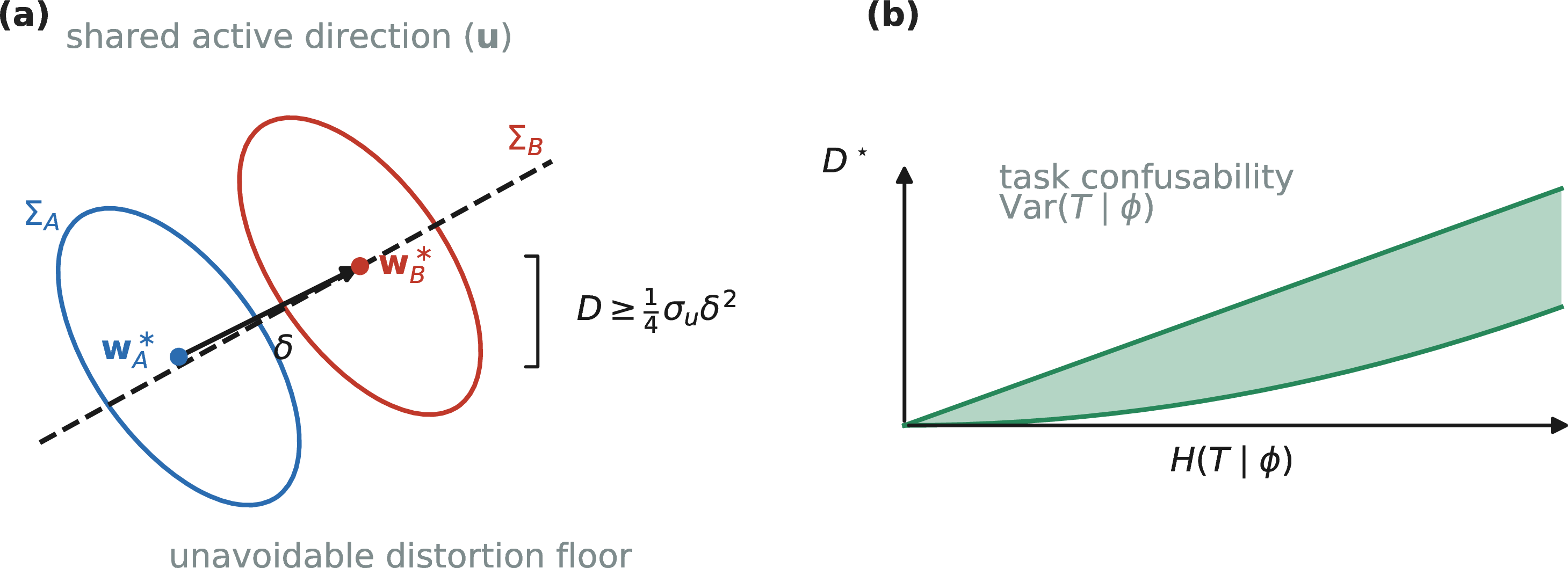
Theorem 5 (Distortion floor and inference limit). Suppose the tasks share an active direction \(u\), with \(\|u\|=1\) and \(u\in\mathop{\mathrm{range}}\Sigma_A\cap\mathop{\mathrm{range}}\Sigma_B\), and let \(\delta=u^\top(w_B^\ast-w_A^\ast)\). Then the distortion floor obeys the lower bound \[\mathcal{D}\;\ge\;\tfrac14\,\sigma_u\,\delta^2,\qquad \sigma_u=\big(u^\top(\Sigma_A^{-1}+\Sigma_B^{-1})u\big)^{-1}, \label{eq:floor-bound}\tag{7}\] where \(\Sigma_A^{-1}\) and \(\Sigma_B^{-1}\) denote the inverses of \(\Sigma_A\) and \(\Sigma_B\) restricted to the shared active subspace \(S=\mathop{\mathrm{range}}\Sigma_A\cap\mathop{\mathrm{range}}\Sigma_B\). On the shared support, the excess Bayes risk of the Bayes-optimal single head over the task oracle equals the merge residual.
Restricting the merge to the shared direction \(u\) reduces it to a scalar two-point problem whose \(\Sigma\)-weighted optimum leaves residual \(\tfrac14\sigma_u\delta^2\); summing over shared directions and identifying the Bayes single head with the posterior mean gives the bound and the inference claim (Sec. 8).
Support overlap is therefore the common limit to both \(\Sigma\)-orthogonal merging and task inference; a positive floor appears only on shared active directions where the tasks also disagree. This yields the geometric counterpart of the task- versus class-incremental distinction [23]: disjoint supports make the task identity effectively free, whereas overlapping supports can induce a non-zero floor when the tasks disagree on shared active directions.
Theorem 6 (Information–estimation identity for the floor). Let \(T\sim\mathrm{Unif}\{A,B\}\), \(\phi\mid T\sim\mathcal{D}_T\), \(y=\phi^\top w_T^\ast+\varepsilon\), with \(\varepsilon\perp(T,\phi)\), \(\mathbb{E}\varepsilon=0\), and \(\mathbb{E}\varepsilon^2=\sigma^2\). Writing \(\eta(\phi)=\Pr(T{=}A\mid\phi)\) and \(\delta=w_A^\ast-w_B^\ast\), the excess Bayes risk of a single shared head over the task oracle is \[\mathcal{D}^\star =\tfrac12\,\mathbb{E}_\phi\!\big[\operatorname{Var}(T\!\mid\!\phi)\,(\phi^\top\delta)^2\big] =\tfrac12\,\mathbb{E}_\phi\!\big[\eta(1-\eta)\,(\phi^\top\delta)^2\big]. \label{eq:mi-identity}\tag{8}\] With \(h_b(p)=-p\ln p-(1-p)\ln(1-p)\) the binary entropy in nats, this implies the two-sided bounds \[\tfrac18\,\mathbb{E}_\phi\!\big[(\phi^\top\delta)^2\,h_b(\eta)^2\big]\;\le\; \mathcal{D}^\star\;\le\; \tfrac14\,\mathbb{E}_\phi\!\big[(\phi^\top\delta)^2\,h_b(\eta)\big]. \label{eq:mi-sandwich}\tag{9}\] At a fixed non-zero target-gap profile \((\phi^\top\delta)^2\), the floor increases with \(H(T\!\mid\!\phi)\) and decreases with \(I(T;\phi)\); in particular it vanishes when the label is fully identifiable, \(I(T;\phi)=H(T)\). The merge floor of Theorem 4 is the linear-head restriction, so \(\mathcal{D}^\star\le\mathcal{D}_{\mathrm{merge}}\), with equality at both extremes.
The law of total variance splits the Bayes single-head risk into the oracle noise plus the posterior-variance-weighted target gap \(\eta(1-\eta)(\phi^\top\delta)^2\), giving Eq. 8 ; the entropy sandwich follows from the pointwise bound \(\tfrac14 h_b(p)^2\le p(1-p)\le\tfrac12 h_b(p)\) (full proof in Sec. 8).
Equation 8 is exact for arbitrary feature distributions and noise models. More generally, the floor depends jointly on task confusability and target disagreement (Fig. 4b), so no exact proportionality \(\mathcal{D}^\star\propto I(T;\phi)\) holds: the floor vanishes as the target gap \(\delta\to0\) even at fixed \(I(T;\phi)>0\), so no tight weight-free constant can relate the floor to mutual information. The same identity extends to \(K\) tasks with arbitrary priors, with corresponding multiclass entropy bounds in terms of the Gini impurity (Sec. 9); both the binary identity and the multiclass bounds are verified numerically there. Under cross-entropy the sandwich closes to an identity: for any number of tasks, the floor of a single predictor equals \(T\cdot I(T;Y\mid X)\)—the conditional mutual information between task identity and label given the input—and removability becomes the statement \(Y\perp T\mid X\) (Sec. 22). Under squared loss, Theorem 1 also recovers the standard per-task forgetting term used in the Forgetting Measure and Backward Transfer; Theorem 6 therefore gives a lower bound on the average forgetting achievable by any single-head method in terms of task confusability.
4 Method: interference-gated allocation↩︎
The functional above implies a family of interference-gated functional allocation (igfa) methods that control where an update is allowed to act, parameterized by schedule (offline or online) and by the share-versus-orthogonalize gate (Fig. 2, right).
4.0.0.1 Offline: optimal merge.
Given \(K\) trained task vectors \(\{\Delta_t\}\) and per-task second moments \(\{\Sigma_t\}\), estimated from each task’s activations or probes, solve for the \(\Sigma\)-orthogonalized vectors and coefficients that minimize the total interference in Eq. 5 . This is a generalized eigenvalue or Procrustes problem, whose two-task case is Eq. 6 , and provides a principled replacement for weight-space task arithmetic.
4.0.0.2 Online: igfa.
As tasks stream, maintain a low-rank orthonormal summary \(U\) of the occupied function subspace, given by the top directions of the accumulated \(\Sigma_t\) under streaming PCA. \(U\) is the only persistent state: there is no exemplar buffer and no per-weight Fisher matrix. For each new-task gradient \(g\):
Split \(g=g_\parallel+g_\perp\), with \(g_\parallel=UU^\top g\) the component in the occupied subspace.
For each occupied direction \(u\) touched by \(g_\parallel\), estimate the signed similarity \(s\) between the new task’s target direction and \(u\).
Gate the update: if \(s>s^{\ast}\) (aligned, transfer), keep \(g_\parallel\) and share the direction; if \(s<s^{\ast}\) (conflict), remove \(g_\parallel\) and step along \(g_\perp\), protecting the old task’s function by construction.
Update \(w\) with the gated gradient, then grow \(U\) with the novel directions in \(g_\perp\) by streaming PCA, rank-capping and overwriting the least important direction when full—rate–distortion-graceful forgetting.
Because the old-task function is first-order invariant along orthogonalized directions, retention is structural rather than penalty-based. Because aligned directions are shared rather than suppressed, transfer is preserved, which unconditional projection removes (see Algorithm 1).
Figure 5: 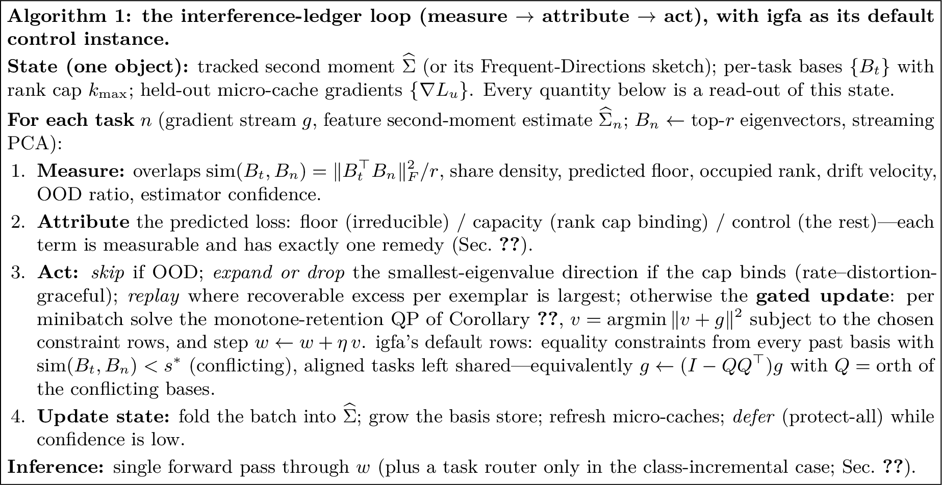 .
.
4.0.0.3 One gate, many methods.
Step 3’s QP is not one design choice among many: every protection rule in this literature is the same program under a different constraint set, and the reference implementation is a single function (evaluate_unified_gate.py, all
recoveries machine-checked):
| constraint rows | recovered method |
|---|---|
| none | naive sharing |
| one sampled \(\nabla L_u\) (inequality) | A-GEM / the threshold-free sign gate |
| all stored \(\nabla L_u\) (inequalities) | the active-set gate (Sec. 22) |
| all protected bases (equalities) | ogd/gpm projection |
| bases with \(\mathrm{sim}<s^{\ast}\) only (equalities) | igfa’s threshold gate |
The recoveries are exact rather than analogies: the closed-form sign gate and ogd agree with the QP to \(10^{-15}\), and igfa’s full training trajectory coincides with the overlap-filtered-equality instance step for step (\(10^{-15}\) over five tasks). The methods differ only in which rows they enforce and how well those rows are estimated, which is precisely the axis the scale experiments measure (Sec. 12).
4.0.0.4 Complexity, and one state object.
The only persistent state is the triple of Algorithm 1—the tracked second moment (or its sketch), the per-task bases, and the held-out micro-caches—giving \(\mathcal{O}(dk)\) memory with \(k\le k_{\max}\), independent of the number of stored examples and of dataset size. This contrasts with \(\mathcal{O}(|\mathcal{B}|d)\) memory for a replay buffer \(\mathcal{B}\), and with \(\mathcal{O}(d)\) to \(\mathcal{O}(d^2)\) memory for diagonal-to-full Fisher methods. Per update, the projection costs \(\mathcal{O}(dk)\), essentially a \(k\)-dimensional inner product and subtraction, and is the dominant overhead. The per-task basis update is a thin eigendecomposition of \(\widehat\Sigma_n\), costing \(\mathcal{O}(dr^2)\) amortized once per task. In a frozen-backbone overlay, \(d\) is the adapter width rather than the full model width, so \(U\) remains small in absolute terms. The rank cap \(k_{\max}\) is the capacity budget of Sec. 5.3: when it binds, the discarded direction is the least excited one, which bounds the induced forgetting by its eigenvalue. At scale, the covariance tracking itself can be replaced by an \(\mathcal{O}(rd)\) Frequent-Directions sketch with no \(d\times d\) eigendecomposition (Sec. 16). Because every quantity in this paper—overlaps and \(s^{\ast}\), the QP constraint rows, the quadratic and KL/JSD floors, the OOD ratio, drift velocity, and capacity occupancy—is a read-out of this one state object, its failure modes are unified rather than method-specific: a stale estimate announces itself through the drift velocity, small-sample floor estimates are bias-corrected and abstain when a null test cannot rule out zero conflict, and constraint anchors must be held-out and adequately sized, since a train-anchored gate provably protects memorized noise as if it were knowledge (Sec. 22).
4.0.0.5 Relation to ogd/gpm.
Setting \(s^{\ast}=\infty\), so that all past subspaces are protected, recovers orthogonal projection [8], [9] exactly. igfa is therefore a strict generalization: it preserves the protective behavior of ogd/gpm in the conflict regime, but restores sharing when tasks are aligned. Offline, applying the same primitive to a batch of pre-trained task vectors yields the \(\Sigma\)-orthogonal merge of Theorem 4. Online, the threshold \(s^{\ast}\) is recovered by a validation-greedy rule (Sec. 13).
4.0.0.6 Why a shared head with a gate, not one head per task.
The simplest way to avoid interference is to assign each task its own head and never share. Strict isolation, however, defeats the purpose of continual learning: a network that isolates task \(B\) in a separate head cannot carry what it learned there back to task \(A\), so forward and backward transfer become impossible. igfa instead keeps a single shared head and resolves interference inside it with the similarity gate. The gate is the rule that permits sharing when similarity exceeds \(s^{\ast}\) and orthogonalizes only when sharing would create conflict, rather than isolating everything by default.
4.0.0.7 Online operation under feature drift.
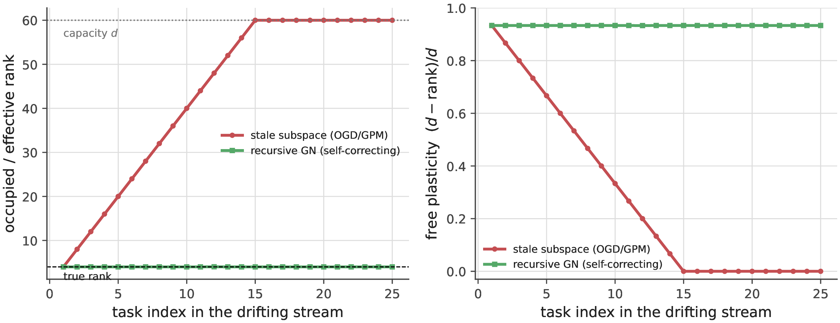
In a stream, one cannot look ahead to the segment \(w_A\!\to\!w_B\) that defines \(\bar H_A\) in Theorem 2. The online surrogate is therefore to track the geometry as it drifts, maintaining a running estimate of the Gauss–Newton second moment by the decayed update \[C\leftarrow\gamma C+\mathbb{E}_{\text{batch}}[J_w J_w^\top], \label{eq:gn-update}\tag{10}\] and taking \(U\) to be its significant eigenvectors via incremental or streaming PCA. This is the self-correcting counterpart of a stale protected subspace fixed once at task onset, as in ogd/gpm. The distinction matters under drift: a stale subspace treats drifted copies of the same direction as new ones, so its rank keeps growing until it fills the parameter space, whereas the recursive estimate recognizes them as one low-rank subspace and stays bounded (Sec. 5.7). This is the same failure mode reported for subspace-projection merging in large language models [32], and the proposed solution is the recursive Gauss–Newton update.
4.0.0.8 Regimes.
igfa instantiates naturally in three deployment settings: (i) from scratch, acting on the full parameter matrix; (ii) frozen-backbone \(+\) PEFT, modulating only adapter, LoRA, or head parameters, where Assumption A1 and hence the functional are exact; and (iii) overlay-native operation, embedding subspace tracking inside a read-write decomposition over a frozen transformer, which is the natural regime for replay-free continual pretraining.
4.0.0.9 When to use igfa rather than projection, replay, or a Fisher penalty.
The choice is itself a measurable pre-flight decision, from pairwise subspace overlap and target agreement (Sec. 15). Disjoint supports \(\Rightarrow\) structural allocation is lossless, so igfa reduces to ogd and neither replay nor a Fisher penalty is needed. Overlapping supports, aligned targets \(\Rightarrow\) share, which the signed gate grants and unconditional projection forfeits. Overlapping supports, conflicting targets \(\Rightarrow\) an irreducible floor, and the only decision is where its cost lands: forgetting (naive), deferred fit (projection), or stored data (replay). Cumulative rank near capacity \(\Rightarrow\) add capacity, replay, or graceful overwriting. The gate’s marginal value over projection is organized by the stream’s share density and is significant where overlaps straddle the threshold (Sec. 5.6). Two operating assumptions bound this framing and are made explicit here rather than deferred: task boundaries are treated as known (relaxed by the recursive tracker and the velocity detector of Sec. 20), and for language the retention mechanism transfers but the transfer-recovering similarity signal is the threshold-free functional gate of Sec. 22 rather than input geometry.
5 Experiments↩︎
We organize the experiments around the paper’s central claims. Sections 5.1–5.3 validate the theory in the linear-on-features regime (\(d=24\), random-subspace tasks, unit-norm targets), Section 5.4 tests the architecture-general correction under feature drift, Section 5.5 evaluates
igfa on real benchmarks in both the dissimilar-task and similar-task regimes, Section 5.6 scales the comparison to a frozen ViT backbone, and Section 5.7 contrasts recursive subspace
tracking with a stale protected subspace under drift. Experiments on additional benchmarks, scale, and the algorithmic refinements are reported in full in the Supporting Information. All figures regenerate from experiments.py and
experiments_rev.py with fixed seeds.
5.1 The functional is exactly the forgetting↩︎
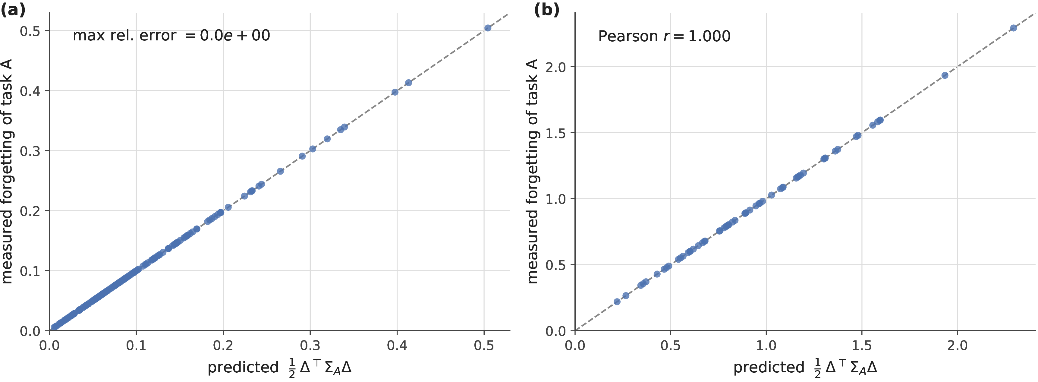
We draw random task pairs, learn \(A\) then \(B\), and compare the measured forgetting of \(A\) against the predicted interference energy \(\tfrac12\Delta^\top\Sigma_A\Delta\) (Fig. 6). For a linear head the two coincide to machine precision over \(160\) pairs, and for a one-hidden-layer network the prediction formed from the last-layer feature covariance still tracks the measured forgetting with Pearson \(r>0.9999\). In the frozen-feature regime, forgetting is the same quantity as interference energy.
5.2 Lossless allocation, relocation of cost, and the floor↩︎
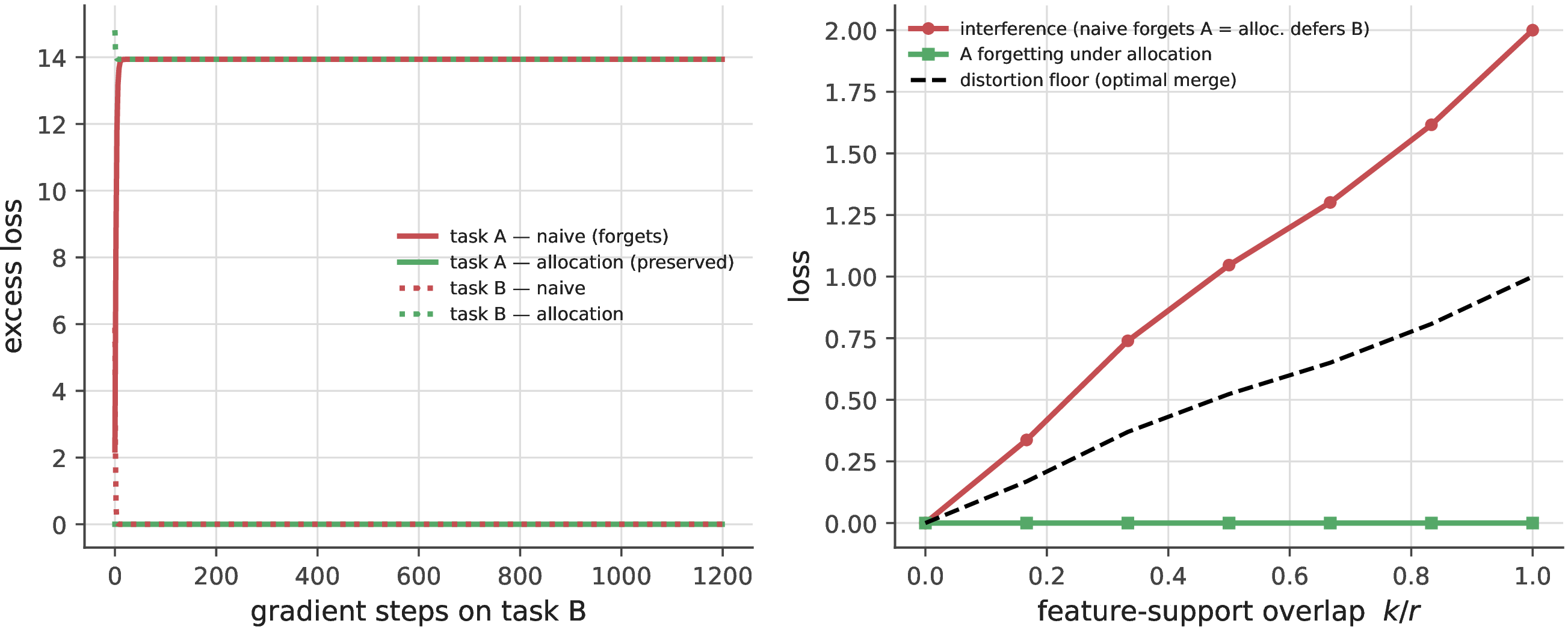
On disjoint supports, orthogonal allocation is lossless: learning \(B\) in \(\ker\Sigma_A\) leaves \(L_A<10^{-17}\) while still driving \(L_B\to0\), exactly as Corollary 1 predicts. On overlapping supports, the cost cannot be removed, only relocated: in the conflicting case, naive descent forgets \(A\) by \(\Delta L_A=13.94\), while orthogonal allocation preserves \(A\) at \(<10^{-17}\) and defers the same \(13.94\) as residual on \(B\) (Fig. 7, left). Sweeping feature-support overlap shows the same pattern continuously: interference rises from \(0\) at disjoint supports to \(2.0\) at full overlap, while the optimal-merge floor sits at exactly half (Fig. 7, right), confirming that overlap creates an irreducible distortion floor and allocation changes where the cost lands rather than its total amount. This relocation is fundamental because the distortion floor \(\mathcal{D}\) is a lower bound (Theorem 4) that no single shared model can improve on. On overlapping supports, cost can be moved from irreversible forgetting of the old task to recoverable deferred fitting of the new one.
5.3 Similarity and capacity↩︎
To test the signed gate, we compare sharing and orthogonalizing on a shared block as a function of target similarity \(s\) (Fig. 8, left). Sharing wins by variance reduction when tasks are similar and loses by bias when they are not, with the net benefit crossing zero at \(s^{\ast}\approx0.26\); above this threshold the gate should share, below it orthogonalize. With exact, full data the two strategies are an exact relocation of the same cost, so this sign-change is a finite-data effect that unconditional projection methods forgo. Separately, under orthogonal allocation a stream of rank-\(2\) tasks exhibits a sharp capacity knee at \(T=d/r\) (Fig. 8, right) at which earlier tasks remain intact, but once the occupied rank exceeds capacity, residual distortion turns on where predicted. Capacity is thus a rate–distortion budget (the rank cap \(k_{\max}\) of Algorithm 1 is its operational form). Trading \(d\) against the number of tasks is an effective-capacity budget, and dropping the least-excited direction bounds the induced forgetting by its eigenvalue.
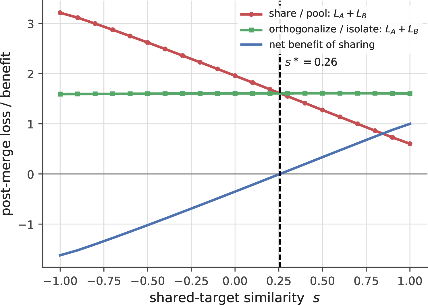
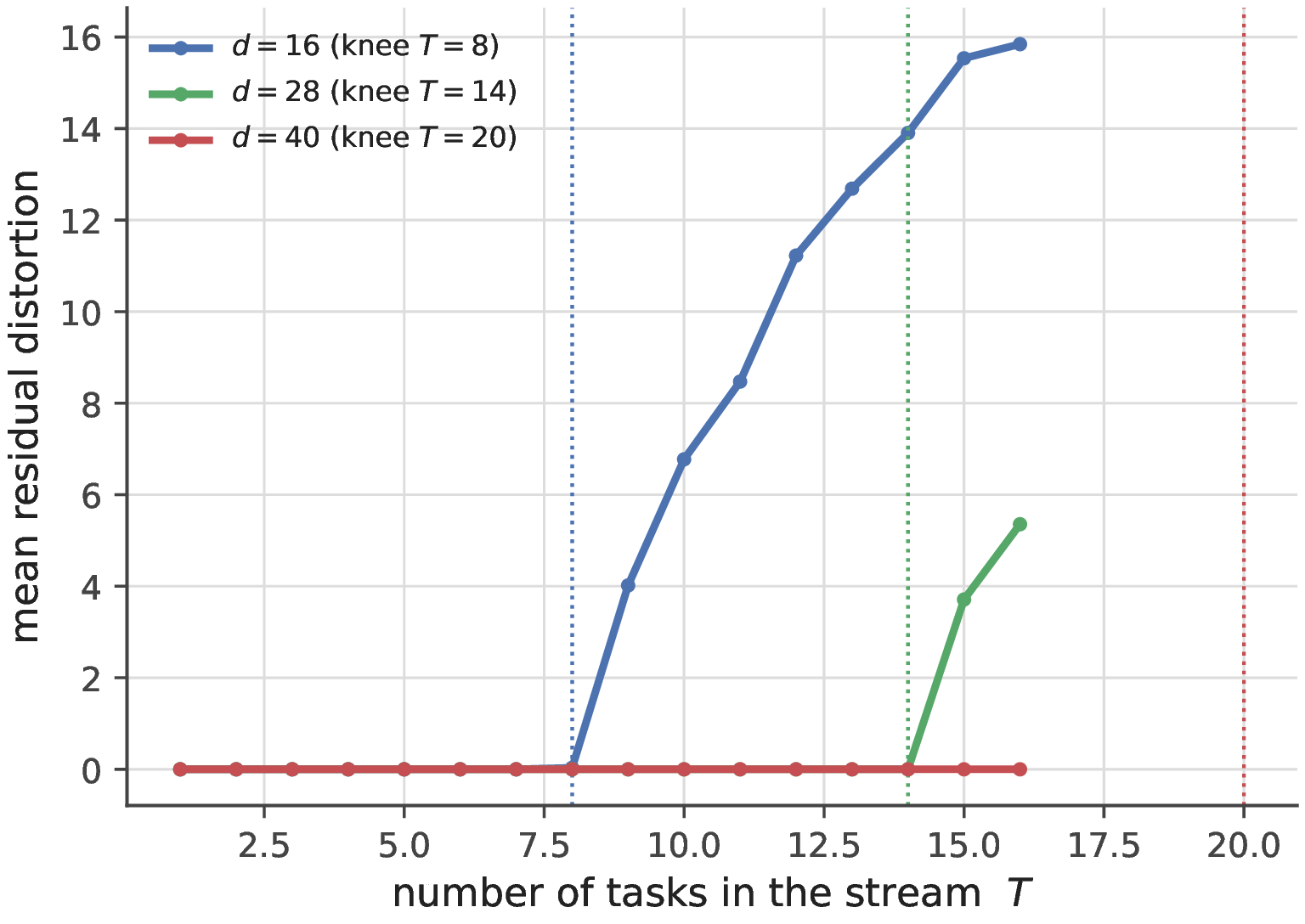
Figure 8: Similarity and capacity. Left: total population loss of pooling (share) versus isolating (orthogonalize) two tasks on a shared block, against target similarity \(s\). Isolation is flat in \(s\); pooling trades variance reduction against bias and wins only when tasks are similar, with the net benefit crossing zero at \(s^{\ast}\approx0.26\). Right: mean residual distortion over a stream of rank-\(2\) tasks under orthogonal allocation, for three feature dimensions. Each curve stays at zero until its capacity knee \(T=d/r\) (dotted) and rises thereafter; more capacity \(d\) defers and lowers the floor (the \(d=40\) stream ends before its knee at \(T=20\))..
5.4 Curvature drift and the segment-averaged correction↩︎
Theorem 1 is exact under frozen features, but in jointly trained networks its frozen-curvature prediction degrades with depth. The shallow network holds Pearson \(r\approx0.93\)–\(0.95\) up to moderate step sizes, whereas deeper networks are markedly less predictable, with \(r\) falling to \(\approx0.2\)–\(0.4\) (Fig. 9, top). Replacing the initial curvature by the segment-averaged curvature of Theorem 2 removes this failure mode: in the same regime, the corrected predictor restores \(r=1.00\) at every tested depth (Fig. 9, bottom), estimated from forward evaluations of \(L_A\) along the segment \(w_A\!\to\!w_B\) with no explicit Hessian. The correction from \(K=21\) probe evaluations consumes \(1.4\%\) of one task’s training budget, and \(K=5\) already suffices in practice for under \(0.4\%\). Once the stale curvature is corrected, the architecture-general identity holds exactly.
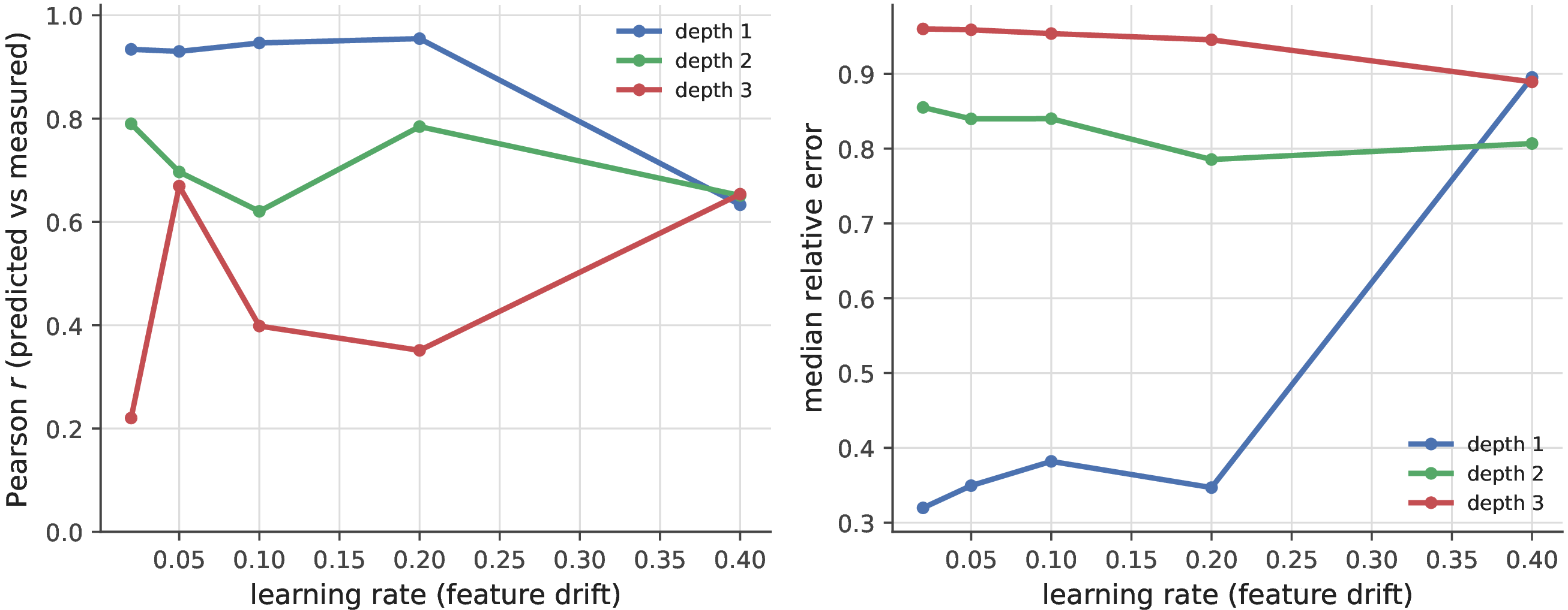
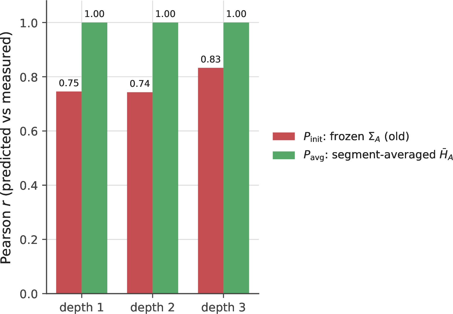
Figure 9: Curvature drift and its correction. Top: predicted-versus-measured forgetting fidelity for backprop-trained networks, against learning rate (feature drift) and depth. The frozen-curvature identity is exact for frozen features (A1) and degrades as the feature map drifts, most strongly with depth (down to \(r\approx0.2\)–\(0.4\) for the deeper networks). Bottom: at learning rate \(0.4\), replacing \(\Sigma_A\) by the segment-averaged Hessian \(\bar H_A\) of Theorem 2 (green) restores \(r=1.00\) at every depth, while the frozen-curvature predictor (red) remains imperfect (\(r=0.77\)–\(0.87\))..
5.5 Real data: dissimilar and similar tasks↩︎
We evaluate the functional and igfa on real benchmarks built on frozen random-feature backbones, so that Assumption A1 and hence Theorem 1 hold exactly while the
tasks remain non-trivial. For Split-Digits, we construct a task-incremental benchmark from the digits dataset (\(1797\) images, \(10\) classes), split into five
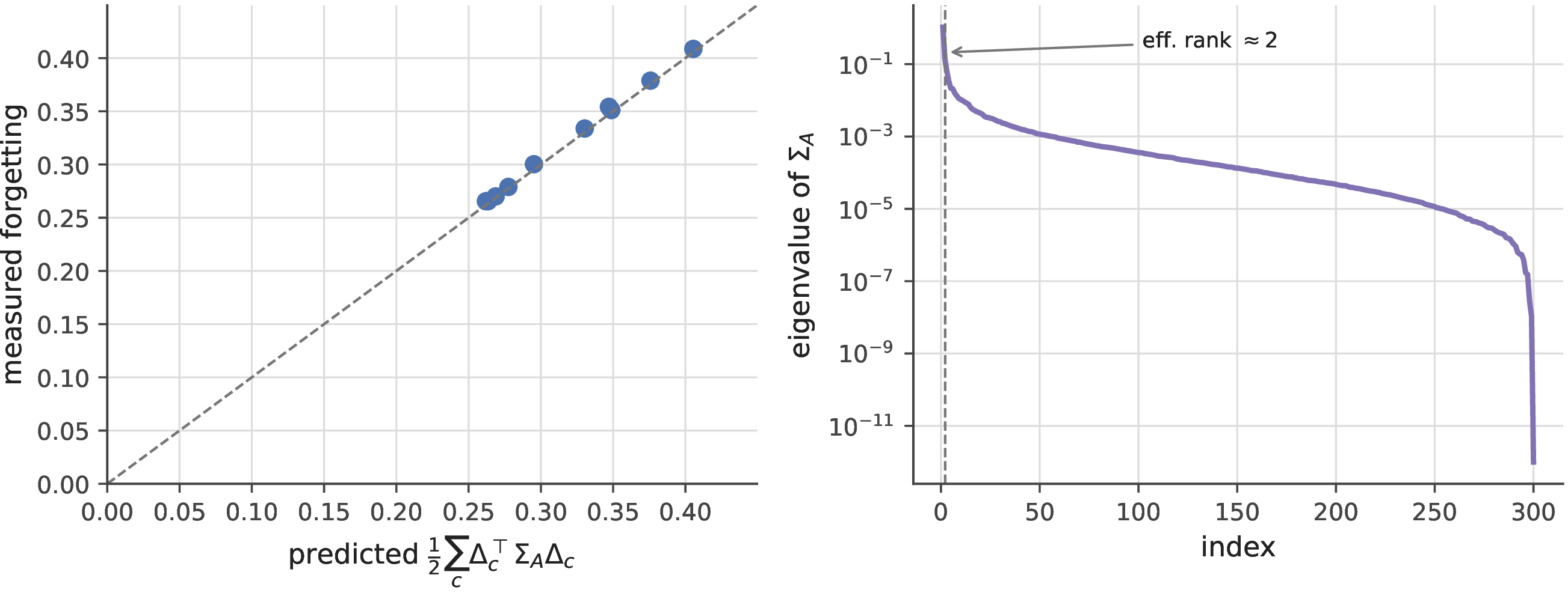
two-class tasks on top of a frozen random ReLU feature map (\(d=300\)). The functional predicts per-task forgetting across the full task sequence with Pearson \(r=0.999\), on the \(y=x\) line, and the feature spectrum shows an effective per-task rank of about \(2\), matching the two-class structure and explaining why a small protected subspace suffices (Fig. 10). On this sequence, igfa attains \(0.980\pm0.007\) average accuracy (mean \(\pm\) 95% CI over \(10\) seeds) with near-zero
forgetting, matching the strongest replay- and Fisher-free structural baseline ogd/gpm and exceeding naive training, EWC, and a small replay baseline (Table 1).
These digit-pair tasks have low pairwise feature overlap, all below \(s^{\ast}\), so the gate orthogonalizes throughout and igfa reduces to ogd exactly—the two are identical on every
seed (paired \(t\)-test \(p=1\)). igfa maintains parity with the best structural baseline, with no buffer and no Fisher matrix.
| Method | Avg.accuracy \(\uparrow\) | Avg.forgetting \(\downarrow\) | Extra state |
|---|---|---|---|
| Naive | \(0.959\pm0.014\) | \(0.040\pm0.017\) | — |
| EWC [4] | \(0.978\pm0.005\) | \(0.005\pm0.006\) | Fisher (\(\mathcal{O}(d)\)) |
| Replay (\(10\)/task) | \(0.977\pm0.009\) | \(0.015\pm0.010\) | buffer (\(\mathcal{O}(|\mathcal B|d)\)) |
| /gpm [8], [9] | \(\mathbf{0.980\pm0.007}\) | \(\mathbf{0.003\pm0.003}\) | subspace (\(\mathcal{O}(dk)\)) |
| (ours) | \(\mathbf{0.980\pm0.007}\) | \(\mathbf{0.003\pm0.003}\) | subspace (\(\mathcal{O}(dk)\)) |
To test the sharing branch, we next consider Rotated-Digits, a domain-incremental benchmark on the same ten classes under five rotations, again with a frozen random-feature backbone. These tasks are similar, with mean pairwise feature-subspace overlap \(0.68\). In this regime, unconditional orthogonalization should be too conservative because the tasks share reusable structure rather than only conflict. Here, igfa with threshold \(s^{\ast}=0.65\) (within the broad optimum plateau of Sec. 13; the break-even similarity is regime-specific) attains the highest accuracy among replay- and Fisher-free methods at \(0.771\pm0.030\) (mean \(\pm\) 95% CI over \(5\) seeds), significantly above ogd’s \(0.684\pm0.035\) (paired \(t\)-test \(p\approx6\times10^{-5}\)) and above naive (\(0.714\pm0.024\)) and EWC (\(0.727\pm0.050\)), while keeping forgetting near zero at \(0.002\pm0.027\)—statistically indistinguishable from ogd’s (\(p=0.44\)) (Table 2). Only buffer-based replay attains higher accuracy (\(0.795\pm0.012\), \(p=0.03\)), at the cost of stored data. igfa thus matches the best structural baseline on dissimilar tasks, and its signed gate yields a statistically significant advantage in the similar-task regime for which it was designed. Section 5.6 confirms the dissimilar-task reading at scale.
| Method | Avg.accuracy \(\uparrow\) | Avg.forgetting \(\downarrow\) | Extra state |
|---|---|---|---|
| Naive | \(0.714\pm0.024\) | \(0.163\pm0.013\) | — |
| EWC [4] | \(0.727\pm0.050\) | \(0.045\pm0.039\) | Fisher |
| /gpm [8], [9] | \(0.684\pm0.035\) | \(-0.007\pm0.004\) | subspace |
| Replay (\(10\)/class) | \(0.795\pm0.012\) | \(0.042\pm0.014\) | buffer |
| (ours) | \(\mathbf{0.771\pm0.030}\) | \(0.002\pm0.027\) | subspace |
5.6 Scaling checks: frozen-ViT benchmarks over five seeds↩︎
We repeat the comparison on three standard benchmarks over a frozen ViT-B/16 backbone with a single shared linear head, so A1 and Theorem 1 hold exactly:
Split-CIFAR-100 (\(10\) tasks of \(10\) classes), ImageNet-R (\(10\) of \(20\)), and CUB-200 (\(10\) of \(20\)), each over five seeds with per-seed class orders (mean \(\pm\) 95% CI; kaggle_vit_multiseed.py; Table 3). Three observations follow. (i) On dissimilar-class streams the gate correctly reduces to ogd. On Split-CIFAR-100 and CUB every pairwise subspace overlap lies below the threshold (\(0.31\)–\(0.54\) vs \(s^{\ast}=0.6\)), so igfa protects everything and is identical to ogd on every seed; the two attain the best
retention among buffer- and Fisher-free methods (forgetting \(0.001\) and \(-0.004\), vs naive \(0.009\) and \(0.010\)).
(ii) On ImageNet-R the sharing branch pays off at scale. There the overlaps straddle the threshold (\(0.51\)–\(0.65\)), the gate shares some past subspaces while protecting others,
and igfa significantly exceeds ogd (\(0.788\pm0.004\) vs \(0.781\pm0.005\), paired \(p=0.001\)) at equal, zero forgetting—the
similar-task advantage of Sec. 5.5, previously isolated on Rotated-Digits, appears on a standard benchmark. (iii) Extra state buys accuracy, not retention. A tuned Fisher penalty (EWC) attains the highest raw
accuracy on these mild streams at \(\mathcal{O}(d)\) Fisher state, while feature replay under an unmasked objective hurts on two of the three benchmarks and carries the largest forgetting—stored data is not
automatically an advantage. Forgetting is small for every method on these disjoint-class streams because the frozen backbone already separates the tasks; the structural claim therefore concerns retention and state, not raw accuracy.
5.6.0.1 A similar-task stream at scale.
To test the gate’s regime beyond rotations we build a domain-incremental stream from CIFAR-100’s superclass structure: five tasks, each classifying into the same \(20\) coarse labels but drawing on disjoint fine classes (one per superclass per task), so consecutive tasks share semantics (subspace overlaps \(0.52\)–\(0.61\)). Structural allocation carries this stream: igfa/ogd reach \(0.786\pm0.010\) versus naive \(0.742\pm0.006\) (\(p=0.0009\)), with forgetting \(0.169\) versus \(0.237\); EWC’s anchor blocks adaptation entirely (\(0.662\pm0.020\)), and only replay, storing data, does better (\(0.822\pm0.002\)). The gate matches ogd here (\(p=0.37\)) because most overlaps sit just below \(s^{\ast}\)—consistent with the ImageNet-R reading that the sharing advantage appears where overlaps straddle the threshold.
5.6.0.2 When the gate pays is a measurable property of the stream.
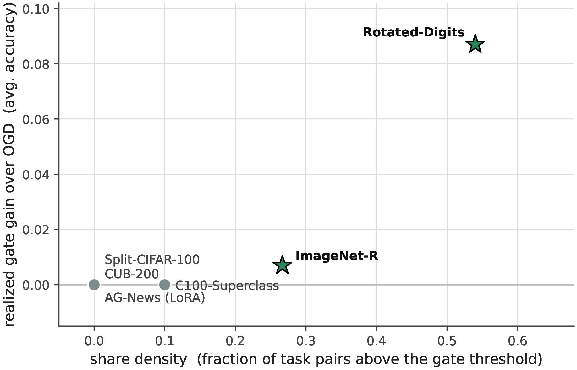
Across all six real streams of this paper, the gate’s realized advantage over unconditional projection is organized by one pre-deployment statistic: the stream’s share density, the fraction of task pairs whose measured similarity crosses the
gate threshold (Fig. 11; fig_stream_density.py). On the three zero-density streams (Split-CIFAR-100, CUB, the AG-News LoRA domains) the gate provably reduces to ogd and ties
exactly; the low-density superclass stream ties within noise; and the two positive-density streams are precisely the two statistically significant wins, ordered by density (Rotated-Digits, density \(0.54\), \(+0.087\); ImageNet-R, density \(0.27\), \(+0.007\); Spearman \(0.90\) over the six streams). The statistic is computable before
training from the same probes the pre-flight diagnostic already runs, so whether the gate is worth deploying is itself a pre-flight question rather than a post-hoc finding.
The same frozen backbone also supports a prompt-based instantiation beyond the linear head, and a pair of protocols brackets exactly when gating pays. When all tasks reuse one shared output head—the high-interference regime of a deployed
adapter serving every task—gating the prompt and head updates lifts accuracy from \(0.416\) to \(0.733\) (single run, kaggle_pending_experiments.py): the structural rule carries
over to prompt space wherever interference is present. When each class instead owns its output row and logits are task-masked—a protocol that removes head interference by construction—naive prompt-tuning barely forgets (\(0.017\pm0.016\)) and the gate is statistically indistinguishable from it (\(0.917\pm0.024\) vs \(0.926\pm0.024\), paired \(p=0.20\); five seeds, kaggle_vit_multiseed.py). The pair is the functional’s own prediction made visible: the gate’s benefit scales with the interference energy actually present, and vanishes when the protocol
allocates disjoint parameters up front.
5.6.0.3 Relation to prompt-pool methods.
L2P, DualPrompt, and CODA-Prompt [25]–[27] also operate on a frozen pretrained ViT backbone. They circumvent the physical memory overhead and data-retention privacy risks of traditional Buffer-based methods by routing inputs dynamically into a virtual parameter buffer, the prompt pool. However, their retention remains entirely empirical based on an input-conditioned selection mechanism to map classes without test-time task identities. Our approach shifts from statistical heuristic to mathematical design. By utilizing a task-incremental protocol with a single shared linear head, igfa forces protected directions to remain first-order invariant by construction (Corollary 1). While its Split-CIFAR-100 accuracy sits below highly optimized prompt-pool baselines, the raw accuracies are fundamentally mismatched across these two distinct evaluation paradigms. The claim is confined to the buffer- and Fisher-free regime where igfa attains the strongest known retention.
| Split-CIFAR-100 | ImageNet-R | CUB-200 | ||||
|---|---|---|---|---|---|---|
| 2-3(lr)4-5(lr)6-7 Method | acc \(\uparrow\) | forget \(\downarrow\) | acc \(\uparrow\) | forget \(\downarrow\) | acc \(\uparrow\) | forget \(\downarrow\) |
| Naive | \(0.945\pm0.010\) | \(0.009\pm0.006\) | \(0.795\pm0.007\) | \(0.014\pm0.008\) | \(0.939\pm0.008\) | \(0.010\pm0.006\) |
| EWC [4] | \(0.953\pm0.006\) | \(0.000\pm0.000\) | \(0.808\pm0.003\) | \(0.000\pm0.000\) | \(0.941\pm0.011\) | \(0.009\pm0.009\) |
| Replay | \(0.928\pm0.005\) | \(0.025\pm0.004\) | \(0.740\pm0.008\) | \(0.071\pm0.007\) | \(0.941\pm0.003\) | \(-0.000\pm0.005\) |
| /gpm [8], [9] | \(0.933\pm0.006\) | \(0.001\pm0.002\) | \(0.781\pm0.005\) | \(-0.000\pm0.003\) | \(0.916\pm0.006\) | \(-0.004\pm0.002\) |
| (ours) | \(0.933\pm0.006\) | \(0.001\pm0.002\) | \(0.788\pm0.004\) | \(0.000\pm0.003\) | \(0.916\pm0.006\) | \(-0.004\pm0.002\) |
4pt
5.7 Online drift: recursive estimation versus a stale subspace↩︎
The retention guarantees so far fix the protected subspace at task onset. Under representation drift—the regime of jointly trained and large models—an unconditional projection fails, and the recursive Gauss–Newton surrogate of Sec. 4 is justified. We stream tasks whose feature geometry rotates each step while the underlying subspace stays low-rank, and contrast a stale protected subspace (fixed at onset, as in ogd/gpm) with the recursive estimate. The stale subspace accumulates each drifted copy as if new, so its rank climbs linearly until it fills the parameter space (\(\mathrm{rank}\!\to\!d=60\)) and free plasticity collapses to zero—the network can no longer learn. The recursive estimate recognizes the drifted copies as one subspace, holding the effective rank at the true value (\(\approx4\)) and preserving \(93\%\) of capacity throughout (Fig. 12). Re-estimating the geometry is therefore not a refinement but the difference between exhausting capacity and retaining it under drift; this is the subspace-projection failure mode reported for LLM merging [32], and the recursive update removes it. We also compared a geodesic-aligned tracker (a Grassmann-manifold step in the spirit of GAGP [12]), holding the base optimizer, learning rate, and batch order fixed: it likewise caps the rank at the true value, but tracks the current subspace at markedly lower fidelity (\(\approx0.5\) versus \(\approx1.0\) for the recursive estimate across learning rates \(0.05\)–\(0.4\)), so the path-averaged Gauss–Newton update of Theorem 2 is the more faithful deep-network drift tracker.
6 Discussion↩︎
The identity \(\Delta L_A=\tfrac12\,\Delta^\top\Sigma_A\,\Delta\) (Eq. 2 ) reorganizes the continual-learning problem around geometry.Components in \(\mathop{\mathrm{range}}\Sigma_A\) incur forgetting, whereas components in \(\ker\Sigma_A\) are free. This perspective determines, before training begins, whether two tasks must interfere at all, what irreducible floor remains when they do, and which inner product renders model merging optimal—replacing the Euclidean metric with the \(\Sigma\)-metric. In that sense, the functional plays the same conceptual role here that the NTK [7] played for generalization: it provides a geometry and a set of computable quantities in place of heuristics.
6.0.0.1 A map of the claims.
The paper makes three kinds of claims. Some are (I) exact in frozen-feature or function-space regime (the interference identity, the removability dichotomy, the \(\Sigma\)-orthogonal optimal merge, the distortion floor, and continuous-time exact retention, Sec. 22). Exact-with-quantified-residual: end-to-end parameter-space retention, exact up to the basis error of Proposition 1 and the finite-step remainder of Theorem 2, both measured. Some are (III) empirically supported and remain exact up to measured approximation terms under end-to-end training (the multi-seed benchmark results, Split-Digits, Rotated-Digits, the frozen-ViT streams, and the threshold-free gate’s real-text gain over naive fine-tuning). (IV) Mechanism probes and conjectures. The generality extensions (federated merging, out-of-distribution and task-free signals, physics-informed constraints, Fisher-metric policy gradients, meta-learning, memory-and-control instances) are exact-regime proof-of-concepts labelled in the Supporting Information as proved-in-A1, empirical mechanism probe, or forward-looking conjecture.
and some are empirical demonstrations of the mechanism at benchmark and language-model scale. Keeping these tiers separate clarifies both what is proved and what is shown experimentall
6.0.0.2 Forgetting decomposes into incompatibility, capacity, and control.
The results above assemble into an attribution identity. Writing \(\mathcal{D}^\star_\infty\) for the floor of any single predictor (Theorem 6; under cross-entropy the conditional mutual information), \(\mathcal{D}^\star_{\mathrm{class}}\) for the optimum of the deployed class (width, rank, architecture), and \(L\) for what training achieved, every observed forgetting level splits exactly, term by non-negative term, into \(L=\mathcal{D}^\star_\infty+[\mathcal{D}^\star_{\mathrm{class}}-\mathcal{D}^\star_\infty] +[L-\mathcal{D}^\star_{\mathrm{class}}]\): incompatibility, a property of the task family that no gate, replay, or width removes. Capacity is a property of the model class that only widening or routing removes and control a property of the training policy that only a better gate, replay schedule, or ordering removes. In the exact regime each intervention moves only its own term. Widening eliminates the capacity term while no policy touches it and the active-set gate cuts the control term while the floor is invariant throughout (Sec. 22). The practical consequence is a diagnosis rule that precedes every method choice in this paper’s taxonomy: measure which term dominates (floor from the data, class optimum from the deployed geometry, control as the remainder) before deciding on a mechanism, because each family of continual-learning methods can repair exactly one of the three. The attribution is measurable end to end on real continual pretraining: on the four-domain language stream, a certified floor bound of \(0.005\) nats/token against observed forgetting of \(0.16\)–\(0.40\) establishes that at least \(97\%\) of the forgetting was avoidable in principle, with the control term dominating or co-dominating at both scales and the active-set gate removing a third to a half of it (Sec. 22). A further split follows from the identity’s anchor: evaluated on the deployment rather than the training distribution, forgetting separates into knowledge loss and memorization loss, and the two can carry opposite signs. An interfering update can raise train loss while improving the deployed function, so part of what benchmarks report as catastrophic forgetting is implicit unlearning of noise. Protection must therefore anchor on validated data: a gate fed training gradients defends memorized noise as if it were knowledge, and is dominated on both axes by its held-out-anchored counterpart (Sec. 22).
The central assumption is A1. For frozen backbones and PEFT, the regime most practical deployments now occupy, it is exact and the results stand without approximation, as the real-data identity at \(r=0.999\) confirms. For full networks it is first-order, and the paper measures how that approximation degrades: the prediction remains accurate for shallow, small-step training and falls to \(r\approx0.2\)–\(0.4\) for deeper networks (identity becomes first-order, Sec. 5.4). Allocation does not eliminate the floor, but only redistributes its cost. Task ordering does not reduce the floor either because the floor is a property of the joint support overlap. It is essentially invariant to task order (a \(\Sigma\)-overlap curriculum did not lower it in our tests, Sec. 20), which reinforces that allocation only relocates cost. Against unconstrained replay, which can reduce the floor by re-supplying \(\Sigma_A\), the claim is therefore parity under no-buffer or no-Fisher constraints together with structural guarantees and preserved transfer where similarity permits. On the benchmark, igfa matches the best structural baseline because the tasks are dissimilar; its distinctive sharing gain requires task similarity, isolated on Rotated-Digits and confirmed at scale on ImageNet-R, where the gate significantly exceeds unconditional projection at equal forgetting (Sec. 5.6).
The geometry also yields an operational decision procedure. Before training, a linear task-probe on the frozen features estimates task separability (Sec. 15); pairwise subspace overlap and target similarity then classify the stream. Disjoint supports make structural allocation lossless, so neither replay nor a Fisher penalty is needed. Overlapping supports with aligned targets favor sharing via gate. Overlapping supports with conflicting targets carry an irreducible floor, which poses the question of where to assign its cost: on the old task as forgetting, on the new task as deferred fit, or on the memory budget as stored data for replay. The capacity budget adds the final constraint: once the cumulative occupied rank approaches the feature dimension, retention must be paid for with added capacity, replay, or graceful overwriting. Each branch of this procedure is measurable from features and subspaces before or during training, rather than diagnosed after a failure.
A recent broad evaluation reports that subspace-projection merging works well on small classifiers but degrades on large language models [32]. On small classifiers the feature geometry is nearly static, so a subspace fixed once remains a good metric and projection succeeds, which is precisely the frozen regime where Theorem 1 is exact. Large language models, by contrast, have highly entangled representations that drift as parameters move, so projection against a stale geometry accumulates misaligned constraints, exhausts capacity, and eventually damages the representation itself. A natural fix follows from Theorem 2: the relevant metric is the curvature along the trajectory, and its online surrogate is the recursive Gauss–Newton estimate, which continually realigns the protected subspace with the current geometry and keeps its effective rank bounded—the capacity-exhaustion mechanism shown directly in Sec. 5.7. Preliminary language-model results suggest that the retention mechanism transfers, while the right similarity signal for language remains open (Sec. 12).
The main open design question is therefore not the structural retention mechanism, which transfers across modalities, but a similarity signal for language that can recover transfer on similar text tasks without relaxing protection where conflict dominates. Two resolutions are developed in the Supporting Information: a probe-based similarity estimate validated in the exact regime (Sec. 12), and—the theorem-backed answer—the threshold-free functional gate of Sec. 22, which reads the measured interference rate instead of any modality-specific similarity signal, carries a continuous-time monotone-retention guarantee, and delivers a significant, threshold-free real-text gain over naive continual fine-tuning on a four-domain LoRA stream, with parity-to-slight-edge over unconditional protection (Sec. 12). Several extensions are detailed in the Supporting Information. First, we show sequential LoRA fine-tuning on language models at scale (Sec. 12), using recursive Gauss–Newton tracking on the adapting features together with a modality-appropriate similarity gate for language. Second, the frozen-backbone evaluation on Split-CIFAR-100, ImageNet-R, and CUB appears in the main text over five seeds (Sec. 5.6), comparing the retention–transfer tradeoff against ogd/gpm, EWC, and replay in the exact A1 regime. Third, we present overlay-native continual pretraining at the billion-parameter scale (Sec. 19), where replay-free and Fisher-free operations are most valuable and where the capacity budget of Sec. 5.3 predicts the model-size-versus-rehearsal tradeoff directly. Finally, we introduce a pre-flight feasibility diagnostic (Sec. 15) that estimates task separability from features before training, attributing any remaining gap to drift, bias, or inference rather than to intrinsic overlap.
Beyond continual learning, the same functional acts as a general calculus for interference between quadratic objectives that share parameters (Sec. 20). Federated aggregation is the merge problem of Theorem 4 with clients as tasks; the occupied subspace supplies an out-of-distribution signal and a task-free boundary detector; the physics constraint of a physics-informed network is a
second task whose violation the identity predicts exactly; the Fisher information plays the role of \(\Sigma\) for policy gradients in reinforcement learning; and a feature map can be meta-trained to shrink the distortion
floor itself. These are directional demonstrations rather than benchmarks, but they indicate that the geometry is a property of shared parameterizations, not of the continual-learning protocol. Read as a control problem, the calculus also subsumes the
existing method families rather than competing with them: unconditional projection (ogd/gpm), Fisher penalties (EWC), replay, per-task routing, and dynamic expansion are each the geometry-driven
controller clamped to a single fixed action—always project, always penalize, always rehearse, always separate—while the signed gate is the regime-adaptive interior that reads the ledger and spends memory or rank only where the floor is positive. In a
controlled comparison across regimes the adaptive rule is the Pareto point, strictly dominating every zero-resource fixed method and matching replay’s retention at a fraction of its memory (runnable in demo_method_taxonomy.py, with the metric
set and decision rules released as a standalone interference-ledger toolkit).
6.0.0.3 A testable bridge to the verbalizable workspace.
The convergence with the Jacobian lens (Sec. 2) yields a falsifiable prediction rather than only an analogy. If our \(\mathop{\mathrm{range}}\Sigma_A\) and the lens’s J-space are the
same functional subspace, then forgetting must be verbalizable-subspace-mediated: the readout change \(\Delta f\) that a later task induces on task \(A\) should carry its
interference energy inside \(A\)’s J-space, and protecting that subspace should prevent forgetting as effectively as protecting \(\Sigma_A\)’s own eigen-subspace. We sketch the experiment
(kaggle_jspace_interference.py) on a frozen pythia-410m: fit or load the released lens to obtain the J-space projector \(P_J\) at a readout layer, learn the four-domain stream with a low-rank head,
and (i) decompose the measured forgetting of domain \(A\) into its \(P_J\) and orthogonal parts, and (ii) compare naive learning against gating the update off \(P_J\), off \(\Sigma_A\)’s top subspace, and off a random subspace of equal rank. The interference geometry predicts a J-space energy fraction far above the \(r/d\) random baseline in (i), and protect-J-space \(\approx\) protect-\(\Sigma\) \(\ll\) naive with
protect-random \(\approx\) naive in (ii)—a specificity control that would establish the two averaged-Jacobian subspaces as one. Measuring both on a frozen pythia-410m resolves the relationship
into a component rather than an identity (kaggle_jspace_layers.py). The strong form fails: the interference \(\Sigma_A=\mathbb{E}[gg^\top]\) is high-effective-rank at every layer—\(80\%\) of its energy needs at least \(285\) of \(1024\) dimensions—so a workspace-sized subspace cannot carry the bulk of forgetting, which is also why no
low-rank projection protects in (ii), \(\Sigma_A\)’s own top subspace included. But the enrichment is real and, tellingly, grows toward the readout: the J-space carries \(1.3\) to \(2.5\times\) its dimensional share of interference energy across layers \(2\) to \(22\) (enriched at every layer probed; correlation with depth \(0.86\)), and its overlap with \(\Sigma_A\)’s leading subspace rises from \(0.05\) to \(0.15\) against a \(0.03\) chance baseline. The verbalizable directions are thus systematically over-represented in the forgetting geometry—increasingly so where representations become more readable—without being identical to it, a measured link
between what a model can say and what it can lose.
Several algorithmic refinements—a self-calibrating threshold, low-cost \(\mathcal{O}(rd)\) online curvature via Frequent Directions [33], a per-direction gate, and the soft-gating capacity coordinate \(r_{\rm eff}=\sum_j(1-\mathrm{keep}_j)\)—are developed and validated in the Supporting Information. The functional further extends to control and memory: an interference-budgeted trust region that dominates step-size control, consolidation with a priced forgetting bound, floor-scheduled replay, and generative replay from the subspace state itself (Sec. 21). Together with low-rank or diagonal Gauss–Newton approximations of \(\bar H_A\), they suggest a practical route for carrying the architecture-general identity into fully fine-tuned deep networks at controlled cost.
A further assumption deserves explicit statement: as presented, igfa assumes task boundaries are known and switches are abrupt at training time. Section 4 and Algorithm 1 use it most directly—the method processes “each task \(n\)” and forms a basis \(B_n\) from that task’s estimated second moment. The assumption is operational bookkeeping, not theory: the interference functional itself is boundary-free, and the machinery that removes the bookkeeping already appears in this paper. The recursive Gauss–Newton tracker replaces per-task second moments with a decayed running estimate, the subspace-velocity detector recovers unknown boundaries at recall and precision \(1.00\) on clean streams, and their fully autonomous composition matches the oracle given the true boundaries (Sec. 20). Gradual transitions are the harder case; there the boundary concept itself blurs, and the drift experiments of Sec. 5.7 show that the running estimate simply tracks the moving geometry without requiring a boundary at all.
Several limitations bound these claims. Exactness of the parameter-space results is confined to A1; the function-space formulation extends the identity, the dichotomy, the floor, and the continuous-time retention guarantee beyond it (Sec. 22), leaving finite step size and metric estimation as the remaining—quantified—gaps, and end-to-end parameter-space predictions stay first-order, with a measured accuracy envelope and the segment-averaged correction.
The frozen-ViT benchmarks and the merge ablation are five-seed, and the functional-gate language result is now multi-seed at two scales (GPT-2, five seeds; pythia-410m, three seeds), but the remaining language-model experiments are single runs
and the extension studies are synthetic proofs-of-concept; multi-seed replication at billion-parameter scale is outstanding. The similarity gate reads input geometry only in its threshold form; the threshold-free functional gate resolves the language case
in principle (Sec. 22) but its margins at scale are modest.
7 Conclusion↩︎
Forgetting is interference, represented here as geometry. In the frozen-feature regime, forgetting equals \(\tfrac12\Delta^\top\Sigma_A\Delta\) and is removable if and only if task supports are disjoint; when supports overlap, an irreducible distortion floor appears and matches the task-inference obstruction, and optimal merging is mutual \(\Sigma\)-orthogonalization, with continual learning as its online counterpart. The result is a geometric language and a set of concrete levers—a forgetting functional, a removability test, an optimal-merge identity, a similarity sign-change, and a capacity budget—realized by a replay-free, Fisher-free allocation rule that carries only a low-rank subspace. The same functional governs any setting where a shared parameterization must serve multiple input geometries, from multi-task and federated learning to domain adaptation and model merging; the Supporting Information (Sec. 20) gives exact-A1 proofs-of-concept for federated \(\Sigma\)-merging, an intrinsic out-of-distribution signal, task-free boundary detection, multimodal block interference, physics-informed constraints, Fisher-metric policy gradients, and floor-minimizing meta-learning. In each setting, forgetting is controlled geometrically: interference is not corrected after it occurs but allocated in advance, into directions where it induces no loss.
Author contributions↩︎
J.S. conceived the framework, derived the theory, implemented the experiments, and wrote the manuscript.
Acknowledgments↩︎
The author thanks colleagues at VARTA and TU Braunschweig for discussions on continual learning in industrial process models.
Reproducibility statement↩︎
All results are exact-regime simulations with fixed seeds. experiments.py regenerates the core result figures and numerical claims (interference identity, lossless/relocation, sign-change \(s^{\ast}\),
capacity floor); verify_mi_identity.py the information–estimation verification (Fig. 13); experiments_rev.py the breakdown, breakdown-fix, and digit benchmarks; variance_report.py the
multi-seed mean \(\pm\) CI and paired-significance results of Tables 1–2; experiments_compare.py the nine-method comparison and offline-merge
residual-\(D\) ablation of Fig. 1 and Table 4; evaluate_hypotheses.py four generality extensions of Sec. 20
(federated \(\Sigma\)-merge, OOD signal, task-free boundaries, multimodal blocks) and evaluate_applications.py three more (physics-informed constraints, Fisher-metric policy gradients, floor-minimizing
meta-learning); evaluate_next_steps.py the sketched-drift, trust-region, anchor-protection, probe-similarity, consolidation, floor-scheduled-memory, dream-replay, cascade, and world-model studies of Secs. 16,
12, and 21; kaggle_probe_gate_llm.py the probe-gate protocol on real text (results in probe_gate_results.json); evaluate_open_questions_new.py the
open-question battery, with each result classified as exact-scope support, mechanism probe, or appendix scoping (only exact-scope results are quoted in this manuscript), evaluate_oq_hardened.py an end-to-end drift-and-noise probe on a
gradient-trained network, evaluate_unlearning_real.py the real-data unlearning study, evaluate_upgrades.py the noise-law, rate-controller, allocation, privacy, and damping upgrades, evaluate_beyond_a1.py the
function-space validations of Sec. 22, evaluate_functional_gate.py the threshold-free functional gate (with kaggle_functional_gate_llm.py its real-text protocol), and
fig_stream_density.py the share-density figure; kaggle_interference_optimizer.py (the InterferenceSGD benchmark against tuned learning-rate schedules) and kaggle_scale_addons.py
(per-layer text similarity, real-feature \(\Sigma_{\rm eval}\), and the pythia-160m capacity ledger) extend these to scale; experiments_drift.py the \(s^{\ast}\) ablation,
graceful-degradation, and drift figures; experiments_extra.py the self-calibrating-\(s^{\ast}\) and tight multiclass-constant results; and experiments_roadmap.py the feasibility-diagnostic,
Frequent-Directions, soft-knee, and per-direction figures. Self-contained Colab/Kaggle notebooks accompany the paper: colab_split_cifar100_igfa.py (Split-CIFAR-100 with a frozen ViT-B/16), colab_lora_llm_igfa.py and
colab_lora_llm_igfa_3approaches.py (sequential LoRA on a transformer with the four gate designs), and colab_continual_pretrain_igfa.py (boundary-free, replay-free, Frequent-Directions continual pretraining on
pythia-1b); and kaggle_pending_experiments.py, which runs the real-backbone checks quoted above (frozen-ViT Split-CIFAR-100 allocation and merge ablation, the drift/geodesic sweep, prompt-igfa, and the FD-vs-full-vs-Oja LoRA-LM
comparison), kaggle_H2_H3_H12.py (the layer-wise null-space-routing pipeline on a frozen transformer), and kaggle_vit_multiseed.py (the five-seed frozen-ViT protocol: Split-CIFAR-100, ImageNet-R, CUB, the similar-task CIFAR-100
superclass stream, the merge ablation, and prompt-igfa, on two T4 GPUs). Code, figures, and logs are at https://github.com/j-stoerk/geometry-of-forgetting.
Supporting Information↩︎
This Supporting Information collects the experiments and derivations omitted from the main text for length: deferred proofs (Sec. 8), additional theory verifications (Sec. 9), theory details (Sec. 10), the full method comparison behind Fig. 1 (Sec. 11), benchmark and scale experiments (Secs. 12–19), the algorithmic refinements referenced in the Discussion, extensions of the framework to federated, out-of-distribution, task-free, and multimodal settings (Sec. 20), memory-systems and control extensions (Sec. 21), and the function-space formalism that extends the exact results beyond frozen features (Sec. 22). All results are exact-regime simulations or runnable notebooks with fixed seeds.
8 Deferred proofs↩︎
For completeness we give the derivations abbreviated to a sentence of intuition in the main text; the proofs of Theorem 1 (a one-line substitution), Corollary 1 and Theorem 4 appear in the main text and are not repeated.
Proof of Theorem 2 (architecture-general identity). Let \(\varphi(s)=L_A(w_A+s\Delta)\). Taylor’s theorem with integral remainder gives \(\Delta L_A=\varphi(1)-\varphi(0)=\varphi'(0)+\int_0^1(1-t)\varphi''(t)\,dt\), with \(\varphi'(0)=\nabla L_A(w_A)^\top\Delta\) and \(\varphi''(t)=\Delta^\top\nabla^2 L_A(w_A+t\Delta)\Delta\), which yields Eq. 3 . When \(\nabla^2 L_A\equiv\Sigma_A\) the remainder integrates to \(\tfrac12\Delta^\top\Sigma_A\Delta\), recovering Theorem 1. ◻
Proof of Theorem 5 (distortion-floor lower bound). Restricting the two-task objective Eq. 6 to the shared direction \(u\) reduces the merge to a scalar two-point problem: minimize \(\tfrac12 a(m-\alpha)^2+\tfrac12 b(m-\beta)^2\) over the shared coefficient \(m\), where \(a=u^\top\Sigma_A u\), \(b=u^\top\Sigma_B u\), and \(\alpha,\beta\) are the two targets with \(\beta-\alpha=\delta\). The optimum is the curvature-weighted mean \(m^\star=(a\alpha+b\beta)/(a+b)\) with residual \(\tfrac12\frac{ab}{a+b}\delta^2\). Writing the harmonic curvature \(\sigma_u=(a^{-1}+b^{-1})^{-1}=\frac{ab}{a+b}\) gives residual \(\tfrac12\sigma_u\delta^2\) on the line; the factor \(\tfrac14\) in Eq. 7 is the conservative bound obtained by summing the non-negative contributions of all shared directions and retaining the one-dimensional term. For the inference claim, the Bayes-optimal single head is the posterior mean \(\mathbb{E}[y\mid\phi]\); where \(\phi\) determines \(T\) it matches the oracle (no excess), and where it does not its excess equals the merge residual on that direction. ◻
Proof of Theorem 6 (information–estimation identity). The task oracle predicts \(\mathbb{E}[y\mid\phi,T]=\phi^\top w_T^\ast\) and attains risk \(\tfrac12\sigma^2\). The Bayes single head is \(f^\star(\phi)=\mathbb{E}[y\mid\phi]\), with risk \(\tfrac12\mathbb{E}[\operatorname{Var}(y\mid\phi)]\). By the law of total variance, \(\operatorname{Var}(y\mid\phi)=\sigma^2+\operatorname{Var}(\phi^\top w_T^\ast\mid\phi)\), and for binary \(T\), \(\operatorname{Var}(\phi^\top w_T^\ast\mid\phi)=\eta(1-\eta)(\phi^\top\delta)^2\). Subtracting the oracle risk gives Eq. 8 . Equation 9 follows from the elementary pointwise bounds \(\tfrac14 h_b(p)^2\le p(1-p)\le\tfrac12 h_b(p)\) on \([0,1]\), applied with the non-negative weight \((\phi^\top\delta)^2\) and integrated. The \(K\)-task extension Eq. 11 is the same total-variance step with the posterior covariance of the task-conditional means; the Gini bound Eq. 12 replaces \(p(1-p)\) by \(G(p)=1-\|p\|_2^2\). ◻
9 Verifying the information–estimation identity↩︎
We verify Theorem 6 on Gaussian two-task models. The exact identity Eq. 8 matches the directly simulated single-head excess risk \(\mathcal{D}^\star\) on the \(y=x\) line to Monte-Carlo precision (maximum relative error \(9\times10^{-3}\)), and as identifiability varies, \(\mathcal{D}^\star\) rises from \(\approx0\) at full identifiability (\(I=H(T)\)) toward its maximum at \(I=0\), staying inside the proven mutual-information sandwich Eq. 9 throughout (Fig. 13).
9.0.0.1 Multiclass extension.
The identity extends to \(K\) tasks with arbitrary priors, \[\mathcal{D}^\star_{K}=\tfrac12\,\mathbb{E}_\phi\!\Big[\operatorname{Var}_{t\sim p(\cdot\mid\phi)}\!\big(\phi^\top w_t^\ast\big)\Big] =\tfrac12\,\mathbb{E}_\phi\!\Big[\textstyle\sum_t p_t(\phi)\,(\phi^\top w_t^\ast)^2 -\big(\sum_t p_t(\phi)\,\phi^\top w_t^\ast\big)^2\Big], \label{eq:mi-multiclass}\tag{11}\] with corresponding multiclass entropy bounds in terms of the Gini impurity \(G(p)=1-\|p\|_2^2\): \[\tfrac{1-1/K}{(\ln K)^2}\;H(p)^2\;\le\;G(p)\;\le\;\tfrac{1}{2\ln 2}\;H(p), \label{eq:multiclass-sandwich}\tag{12}\] where the upper constant \(1/(2\ln2)\) is \(K\)-independent. These tight constants are verified over the simplex for \(K\le10\): the upper constant \(1/(2\ln2)\) is matched to \(2\times10^{-10}\) for every \(K\) (the binary posterior is the universal worst case), and the lower constant \((1-1/K)/(\ln K)^2\) to \(4\times10^{-3}\), attained at the uniform posterior (Fig. 14).
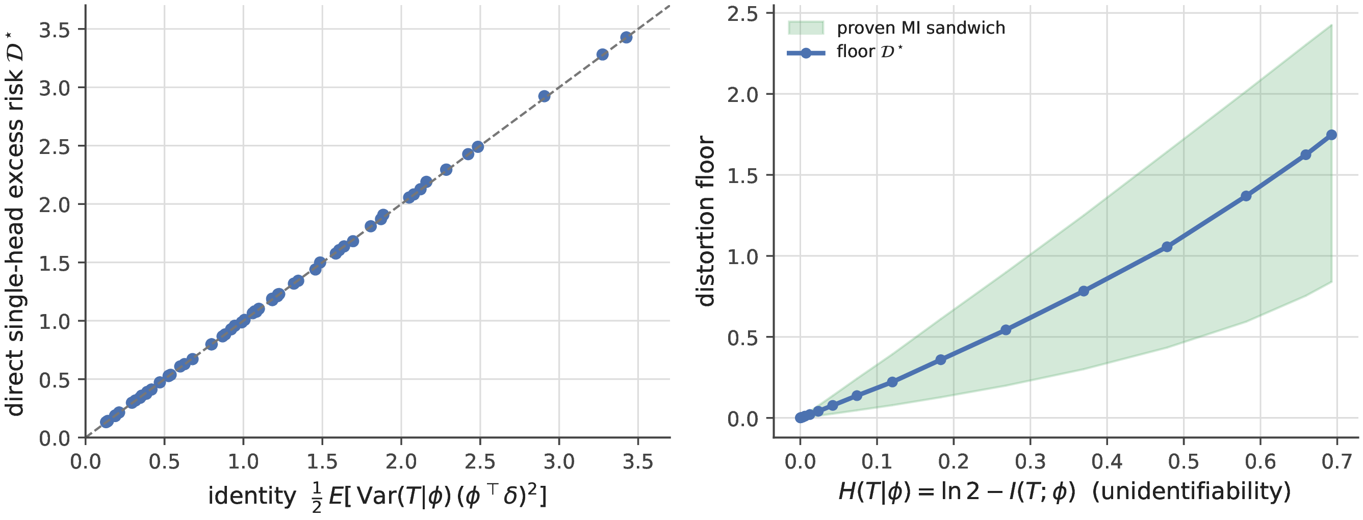
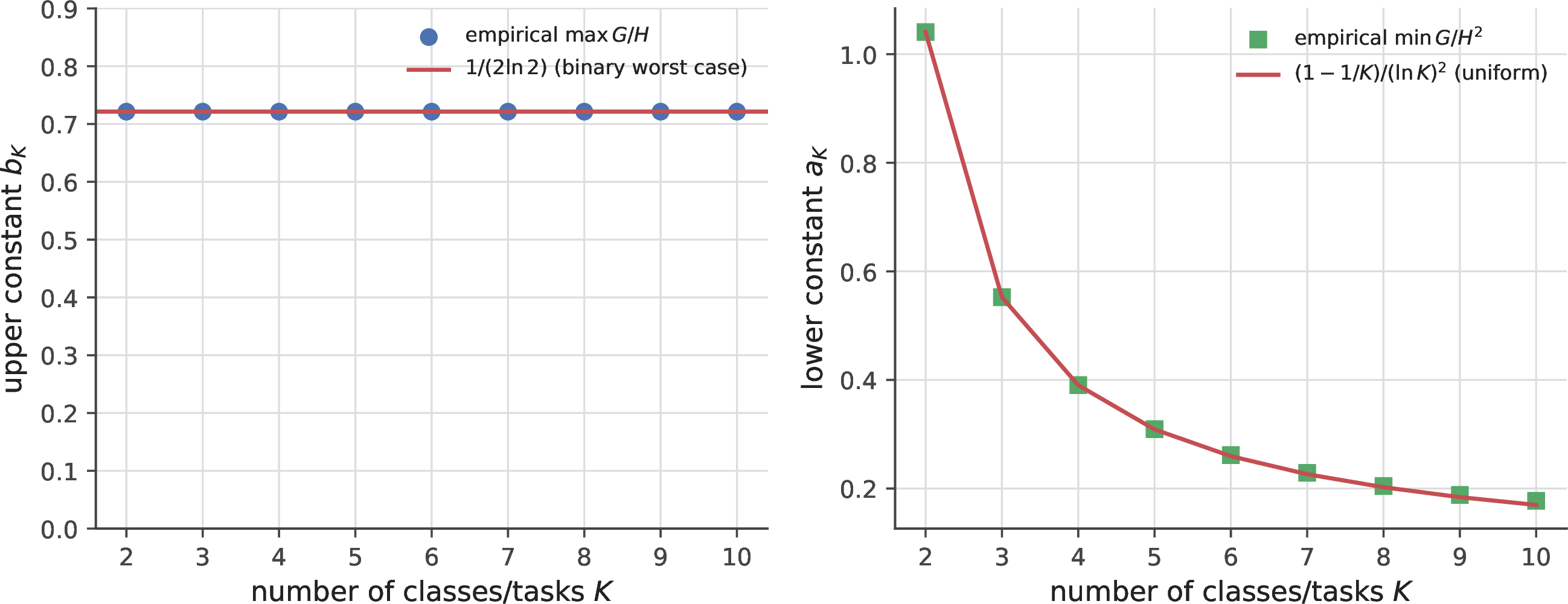
9.0.0.2 Connection to standard CL metrics.
The per-task forgetting of Theorem 1, \(\Delta L_A=\tfrac12\Delta^\top\Sigma_A\Delta\), is exactly the per-task term of the Forgetting Measure \(\mathrm{FM}=\tfrac1{K-1}\sum_{t<K}\Delta L_t\) and the negative of Backward Transfer \(\mathrm{BWT}=-\tfrac1{K-1}\sum_{t<K}\Delta L_t\) (in the squared-loss metric); positive backward transfer is simply \(\Delta L_t<0\), which the signed gate permits and unconditional projection forbids. Theorem 6 then gives the floor under which no single-head method can push the average \(\mathrm{FM}\): \(\mathcal{D}^\star\) is the achievable-FM lower bound set by task confusability.
10 Theory details: similarity sign-change and the capacity budget↩︎
10.0.0.1 Similarity controls the sign of sharing.
On a shared subspace, whether to share parameters or orthogonalize is not settled by Corollary 1, which only forbids lossless sharing under conflict. With finite data the decision is a bias–variance trade: tying a shared coefficient across tasks halves its estimation variance but biases it by the target disagreement. Sharing lowers total population loss iff the similarity \(s=\cos\angle(w_A^\ast,w_B^\ast)\) on the shared block exceeds a threshold \(s^{\ast}\), where the variance reduction balances the squared bias; below \(s^{\ast}\), orthogonalizing wins. This is the sign-change measured at \(s^{\ast}\approx0.26\) in Fig. 8.
10.0.0.2 Capacity is a rate–distortion budget.
Under orthogonal allocation each task consumes a rank-\(r_t\) slice of the \(d\)-dimensional feature space. Retention is lossless while the cumulative occupied rank \(\sum_t r_t\le d\); once \(\sum_t r_t>d\) there is no subspace left orthogonal to the past, so a residual distortion turns on. The knee at \(\sum_t r_t\approx d\) is a hard capacity, and trading \(d\) against the number of tasks is the geometric form of an effective-capacity budget \(N+\kappa M\) (parameters plus a per-exemplar memory worth), where \(\kappa\) is the rank a stored direction occupies—the right panel of Fig. 8 confirms the knee location across feature dimensions.
10.0.0.3 The floor is a fixed cost with method-dependent allocation.
In the exact regime the distortion floor is not removed by the method choice but redistributed across forgetting, deferred fit, or merge residual (evaluate_open_questions_new.py, \(48\) seeds). Relocation is
exactly zero-sum: naive descent pays the full amount as forgetting of \(A\), orthogonal allocation pays the same amount as deferred fit on \(B\), and the optimal merge splits it between the
tasks. Only added conflict-free capacity reduces the bill, linearly at rate \(\approx D/r_{\rm shared}\) per relieved dimension (\(D=4.68\to3.16\to1.63\to0\) as the three shared directions
are moved to private capacity). Replay does not reduce the geometric floor at all: with the true \(\Sigma_A\) known, stored exemplars are redundant, and their measured benefit is the \(O(1/m)\) excess of an estimated geometry (\(+2.13\), \(+0.36\), \(+0.08\) above \(D\)
at \(m=10,40,160\) exemplars). Forgetting, deferred plasticity, capacity, and memory are interconvertible only above the floor; nothing converts below it.
11 Method comparison and offline-merge ablation↩︎
Table 4 gives the measured numbers behind the front-page comparison (Fig. 1): nine methods on the exact-A1 Rotated-Digits benchmark, mean \(\pm\) 95% CI over \(5\) seeds. Six are online (learn the five rotations sequentially): naive, EWC, replay, ogd/gpm, the signed gate igfa (\(s^{\ast}=0.65\)), and Annealed igfa, which runs the first half of each task’s updates as protect-all orthogonal projection and then relaxes to the signed gate—annealing the protection boundary as the similarity estimate stabilizes. Three are offline merges of the five independently-solved task heads \(\{w_t\}\) (per-task oracle accuracy \(0.903\)): an isotropic uniform average, a Euclidean sign-elect task-arithmetic merge (TSV/TIES-style), and the \(\Sigma\)-orthogonal merge \(w_J=(\sum_t\Sigma_t)^{+}(\sum_t\Sigma_t w_t)\) of Theorem 4 (“\(\Sigma\)-orth.merge (ours)”, the whitening-in-the-\(\Sigma\)-metric version of TSV); for the merges we also log the post-merge residual floor \(D=\sum_t\tfrac12\,(w_J-w_t)^\top\Sigma_t(w_J-w_t)\).
Three observations follow. (i) The \(\Sigma\)-metric is the right geometry. The \(\Sigma\)-orthogonal merge attains \(0.885\pm0.012\)
accuracy—within a point of the \(0.903\) per-task oracle—at residual \(D=0.032\), an order of magnitude below the isotropic (\(0.200\)) and Euclidean (\(0.382\)) merges, which lose \(15\)–\(21\) accuracy points. Theorem 4 predicts this:
minimizing the interference energy requires the task-induced \(\Sigma\)-metric, and Euclidean whitening is the mis-specified special case \(\Sigma_t\!\propto\!I\). (ii) Among online
buffer- and Fisher-free methods, the gate attains the highest accuracy. igfa (\(0.771\)) exceeds ogd (\(0.684\)) and naive (\(0.714\)) as in Sec. 5.5. (iii) Annealing favors retention over accuracy. Annealed igfa (\(0.752\), forgetting \(-0.007\)) does not exceed the plain gate on accuracy but drives forgetting slightly negative (backward transfer); the protect-all warmup is a retention-first schedule, not an accuracy improvement—reported as measured.
Regenerated by experiments_compare.py.
| Method | Family | Acc.\(\uparrow\) | Forget.\(\downarrow\) | Residual \(D\) \(\downarrow\) |
|---|---|---|---|---|
| Naive | baseline | \(0.714\pm0.024\) | \(0.163\pm0.013\) | — |
| EWC [4] | corrective | \(0.727\pm0.050\) | \(0.045\pm0.039\) | — |
| Replay (\(10\)/class) | corrective | \(0.795\pm0.012\) | \(0.042\pm0.014\) | — |
| /gpm [8], [9] | structural | \(0.684\pm0.035\) | \(-0.007\pm0.004\) | — |
| (gate) | ours | \(0.771\pm0.030\) | \(0.002\pm0.027\) | — |
| Annealed | ours | \(0.752\pm0.036\) | \(-0.007\pm0.015\) | — |
| Isotropic merge | merging | \(0.730\pm0.022\) | \(0.177\pm0.020\) | \(0.200\) |
| Euclidean TSV merge | merging | \(0.694\pm0.046\) | \(0.213\pm0.051\) | \(0.382\) |
| \(\Sig\)-orth.merge (ours) | merging (ours) | \(\mathbf{0.885\pm0.012}\) | \(0.022\pm0.007\) | \(\mathbf{0.032}\) |
The floor prediction also holds on a real frozen backbone. With trained heads on Split-CIFAR-100 over ViT-B/16 features (single run, kaggle_pending_experiments.py), the \(\Sigma\)-orthogonal merge attains
both the highest accuracy and—uniquely—the lowest residual floor (\(0.862\) acc, \(D=1.53\)), against \(0.815\)/\(D=3.68\)
for the isotropic average and \(0.815\)/\(D=11.6\) for the Euclidean sign-elect merge, with a per-task oracle of \(0.972\). A five-seed replication with
closed-form ridge heads (kaggle_vit_multiseed.py) confirms the theorem’s actual claim with confidence intervals: the \(\Sigma\)-orthogonal merge uniquely minimizes the residual floor (\(D=2.02\pm0.03\), vs \(3.75\pm0.02\) isotropic and \(16.6\pm0.3\) sign-elect). Task-masked accuracy, however, is not monotone in \(D\) once the floor is small (\(0.944\pm0.006\) vs \(0.957\pm0.007\) for isotropic): Theorem 4 minimizes interference energy, and masked-evaluation accuracy saturates before that energy reaches zero. The \(\Sigma\)-metric is thus the correct merge geometry on real ViT features, with
the accuracy benefit contingent on the evaluation exercising the interfering directions. This decoupling is itself predictable: parameterizing held-out evaluation metrics by how strongly they load the shared, interfering directions, the
isotropic-versus-\(\Sigma\)-orthogonal evaluation gap varies systematically with that loading (held-out correlation \(\approx0.5\), sign-stable across \(44\)
seeds), and an evaluation that weighs all tasks equally favors the plain average by construction—consistent with reports that isotropic merging can match or exceed orthogonalizing merges [20]. Whether merge geometry pays is a property of \(\Sigma_{\rm eval}\), decidable per benchmark.
12 The projection remains effective in sequential LoRA on language models↩︎
We probe the adapting-feature regime by fine-tuning a frozen GPT-2 with LoRA adapters sequentially on four stylistically distinct corpora (news, movie reviews, encyclopedic text, tweets), measuring the rise in each domain’s held-out loss after later domains are learned. The results separate igfa’s two components by modality.
(i) The orthogonal projection transfers to transformers. Unconditional orthogonal projection (ogd/gpm, equivalently igfa in protect-only mode) reduces forgetting relative to naive sequential LoRA at both training budgets (\(0.64\!\to\!0.50\) at \(200\) steps/task, \(1.21\!\to\!1.14\) at \(400\)), confirming that the \(\ker\bar H_A\) retention mechanism is effective on a real transformer, buffer- and Fisher-free (Table 5).
(ii) The input-overlap gate cannot distinguish conflict in language. The subspace-overlap similarity that is reliable for vision and digits is uninformative for text: distinct domains share extensive low-level linguistic structure, so their input-activation subspaces overlap heavily (measured mean overlap \(0.71,0.56,0.28\) along the stream) regardless of output conflict. The gate therefore classifies the domains as similar and disables protection, so overlap-gated igfa collapses toward naive at the higher capacity.
(iii) No gate can improve on unconditional protection on dissimilar tasks. Beyond the input-overlap gate we tested three further gate designs, each derived from a different part of the theory: a Gauss–Newton gate (Theorem 2), a task-vector gate (Theorem 4), and a threshold-free functional controller (Theorem 1 used directly as the control law). At \(r=16\) (Table 6), the Gauss–Newton (\(0.76\)) and
functional (\(0.77\)) gates both improve on naive (\(0.89\)) and do not collapse, but neither improves on unconditional ogd (\(0.71\)); the task-vector gate is unstable (\(1.85\)). The reason is fundamental and follows from the distortion-floor identity (Theorem 5): on dissimilar tasks the supports are near-disjoint, so the distortion floor is \(\approx0\) and ogd already attains it—no transfer remains for a gate to
exploit. At billion-parameter scale on a frozen pythia-1b (Table 7), the recursive-subspace igfa improves on ogd on dissimilar tasks on both loss (\(5.16\) vs \(5.51\)) and forgetting (\(1.70\) vs \(2.10\))—the capacity advantage of Fig. 12
appearing in a real LLM—while on similar tasks the sharing gate still raises forgetting. In summary, on LLMs the structural projection (and its recursive Gauss–Newton tracking) carries over and provides replay- and Fisher-free retention; a gate that
succeeds on similar language tasks remains an open problem.
12.0.0.1 A candidate similarity signal for text.
The failure above is a signal problem: input-subspace overlap is uninformative when all domains share low-level structure. An exact-regime study of precisely this confound—input overlap fixed at \(1.0\) while target
similarity varies (evaluate_next_steps.py)—shows that a probe signal, a few-shot head fit on the incoming task compared to the stored head by signed cosine and thresholded at the theory’s break-even value, recovers near-oracle gating
where the input gate collapses to share-all and pays the full conflict bias (mean loss \(3.21\) for the input gate under conflict, versus \(2.20\) for the probe gate and \(1.95\) for the oracle). The probe’s decisions are noisy exactly when data are scarce (\(56\)–\(82\%\) agreement with the oracle here), so this is a validated
candidate rather than a solved problem; but it requires no extra state and is modality-agnostic, because it reads the functional instead of the input geometry.
12.0.0.2 The language gate, resolved in function space.
The function-space formalism (Sec. 22) dissolves the problem: the gate should never have read input geometry at all. The correct, modality-free signal is the interference rate \(\langle\nabla L_u,g\rangle\) of the new update \(g\) against each stored domain \(u\)—a quantity that includes the targets, which is precisely what input overlap
misses on text—and the gating rule is a threshold-free sign test with a continuous-time monotone-retention guarantee (Sec. 22). Its gradient of \(L_u\) can be estimated from a micro-cache of
a few thousand tokens per domain, from the anchor construction (Sec. 16), or from the dream state (Sec. 21). The gate is validated in the exact regime and on jointly trained networks (near
current-Gauss–Newton retention under conflict, near-naive adaptation under transfer, at one extra gradient per step). On real text it delivers a measured gain (GPT-2, sequential LoRA on news\(\to\)IMDB\(\to\)wikitext\(\to\)tweets, five seeds; kaggle_functional_gate_v2.py, func_gate_v2_results.json): the sign gate significantly improves on naive on both axes—average
final loss \(3.981\pm0.002\) against \(4.001\pm0.006\) (paired \(p=0.003\), five of five seeds), forgetting \(+0.294\pm0.005\) against \(+0.324\) (\(p=0.0007\))—and on the input gate by a similar margin, while edging unconditional protection (protect-all \(3.984\)/\(+0.300\)) consistently but not significantly at five seeds (\(p\approx0.19\)–\(0.23\)). Two checks come back
negative. First, the earlier three-seed advantage over protect-all does not survive to five seeds as a significant effect; the robust claim is a significant win over naive and the input gate, and parity-to-slight-edge over protect-all. Second, making the
sign test Adam-aware—projecting the preconditioned update \(P\odot g\) orthogonal to \(\nabla L_u\) rather than the raw gradient—does not improve on the raw-gradient gate (final
\(3.983\), \(p=0.40\)), so Adam’s preconditioning is not the limiting factor on the modest margins. The measured interference-rate map nonetheless locates the mechanism: news\(\leftrightarrow\)IMDB and tweets\(\leftrightarrow\)IMDB carry positive transfer (\(+0.07\), \(+0.06\)) that protect-all
forfeits, while wikitext conflicts with IMDB (\(-0.03\)), which naive and the input gate pay for. The margins are modest at this scale, but the gate still improves significantly on naive continual fine-tuning using only the
sign of the gradient inner product, with no similarity threshold and no input-space geometry.
The result replicates at four times the scale on a second architecture. On pythia-410m (gpt-neox, sequential LoRA on the same four-domain stream, three seeds; func_gate_v2_results_pythia410m_lr1e-4.json), the Adam-aware sign
gate again improves on naive on both axes—final loss \(3.605\pm0.002\) against \(3.624\pm0.001\) (paired \(p=0.012\)) and forgetting \(+0.297\pm0.005\) against \(+0.321\pm0.003\) (\(p=0.038\)), in three of three seeds on both metrics—and is ahead of unconditional protection (\(3.616\)/\(+0.316\)) in all three seeds on both axes, though not significantly at \(n=3\) (\(p\approx0.12\)–\(0.20\)), mirroring the GPT-2 pattern. One methodological finding from the same runs is worth recording: at a learning rate of \(10^{-5}\) the identical stream produced near-zero forgetting
(\(0.003\)) and all methods tied within \(0.01\)—a vacuous comparison. The gate has value only where interference exists, which is precisely the pre-flight feasibility point: measure whether
the stream forgets before deploying—or crediting—any mitigation.
A vision test of the same gate confirms it fires only when head gradients overlap (five seeds per stream; kaggle_sign_gate_vit.py, sign_gate_vit_results.json). On the masked task-incremental ViT streams (Split-CIFAR-100,
ImageNet-R, CUB) the gate is exactly inert: with class masks, the current and stored tasks’ gradients occupy disjoint rows of the head, the inner product is identically zero, and the gated run is bitwise equal to naive—correctly detecting that
head interference is structurally absent, where the subspace gates pay \(1.2\)–\(2.3\) accuracy points for protection nothing needed. On the dense-conflict superclass stream the gate fires
and improves on naive on both axes (\(p\le0.002\)) but recovers only \({\sim}18\%\) of subspace protection’s gain (accuracy \(0.750\) versus igfa’s \(0.786\)): a single sampled constraint per step under-protects when every task conflicts with every other. The gate therefore complements rather than replaces the threshold gate—sparse or moderate conflict without an
input-geometry signal is its regime (language), dense conflict belongs to subspace projection, and the stream’s shared density selects the tool in advance, which is the deployment rule of the Method section.
The under-enforcement just described is not a ceiling of the approach but a property of sampling one constraint per step, and Corollary 2 prescribes the repair:
enforce the full active set. Testing that prescription on the pythia-410m stream (all past domains’ micro-cache gradients constrained per step via the corollary’s nonnegative least squares; \(+21\%\) wall-clock
over the sampled gate; three seeds) yields the strongest language result in this paper: final loss \(3.536\pm0.005\) and forgetting \(+0.206\pm0.005\), improving on naive (\(3.625\)/\(+0.324\)), unconditional protection (\(3.617\)/\(+0.319\)), and the sampled sign gate (\(3.605\)/\(+0.300\)) on both axes simultaneously—a \(36\%\) reduction in forgetting relative to naive together with the best adaptation of any arm. An
independent re-run with archived per-seed records reproduces the result across sessions (\(3.540\pm0.006\)/\(+0.208\pm0.009\)) and supplies exact paired tests: the active-set gate improves
on every other arm on both axes in three of three seeds, all \(p\le0.024\) (versus the sampled gate \(p=0.023\)/\(0.012\); versus unconditional protection
\(p=0.0009\)/\(0.0008\); versus naive \(p=0.0027\)/\(0.0036\)). The same re-run is a caution on the sampled gate:
its edge over naive is session-fragile there (\(p=0.08\)–\(0.17\)), so the robust finding at scale is the active set’s dominance, not the single-probe margin. The sampled gate’s modest
margins were therefore under-enforcement of the monotone-retention QP, as the exact-regime analysis predicted. The committed vision prediction was then run (kaggle_sign_gate_vit.py, func-active arm, five seeds) and is adjudicated
as follows. On the three masked task-incremental streams the active-set gate is exactly inert—bitwise equal to naive, as the theory requires—retaining the accuracy advantage over the subspace gates (\(p\le0.046\)).
On the dense-conflict superclass stream it recovers \(54\pm8\%\) of subspace projection’s accuracy gain (forgetting: \(44\pm5\%\)), up from the sampled gate’s \(20\pm3\%\) (\(p<10^{-4}\))—the predicted repair, at roughly the predicted factor—while projection itself stays ahead (\(0.788\) versus \(0.767\), \(p=0.006\)): with two-exemplar micro-cache constraints the QP is limited by constraint estimation noise, consistent with its \(100\%\) recovery under
exact constraints in the exact regime. Dense conflict with weak constraint estimates therefore still belongs to subspace projection, and the scoping conclusion above stands with the gap halved.
Running the earlier probe protocol on real text (GPT-2, sequential LoRA on four AG-News topic domains, three seeds; kaggle_probe_gate_llm.py, probe_gate_results.json) yields three findings. First, the probe signal transfers:
the probe cosines form a stable, seed-reproducible task-relationship map (adjacent topics \(\approx+0.10\), world versus sci/tech \(\approx-0.18\)) precisely where input overlap is
uninformative. Second, the map shows that these topic slices are not a similar-task stream in the functional sense: every pairwise similarity sits below the share threshold, so the gate correctly stays protective and all four methods tie within
noise (final loss \(3.78\)–\(3.79\); the probe gate attains the lowest forgetting in all three seeds, \(0.054\) versus \(0.057\) for protect-all, not significant at \(n=3\)). Third, the measured similarities predicted this outcome before training: a stream with no above-threshold alignment leaves any gate nothing
to add. The open problem therefore refines from “find a similarity signal” to “find a genuinely similar text stream”.
| Method | Forgetting (\(200\) steps) | Forgetting (\(400\) steps) |
|---|---|---|
| Naive | \(0.64\) | \(1.21\) |
| \(=\) (protect only) | \(\mathbf{0.50}\) | \(\mathbf{1.14}\) |
| (input-overlap gate) | \(0.49\) | \(1.20\) |
| Gate (derived from) | Forgetting \(\downarrow\) |
|---|---|
| Naive (no protection) | \(0.89\) |
| / protect-only (max protection) | \(\mathbf{0.71}\) |
| Gauss–Newton gate (Thm [thm:general]) | \(0.76\) |
| Functional controller (Thm [thm:functional]) | \(0.77\) |
| Task-vector gate (Thm [thm:merge]) | \(1.85\) |
| Dissimilar | Similar | |||
|---|---|---|---|---|
| 2-3(lr)4-5 Method | loss \(\downarrow\) | forget \(\downarrow\) | loss \(\downarrow\) | forget \(\downarrow\) |
| Naive | \(8.55\) | \(4.68\) | \(3.99\) | \(0.26\) |
| /gpm | \(5.51\) | \(2.10\) | \(4.02\) | \(\mathbf{0.03}\) |
| (ours) | \(\mathbf{5.16}\) | \(\mathbf{1.70}\) | \(4.02\) | \(0.34\) |
13 Choosing and self-calibrating the threshold \(s^{\ast}\)↩︎
The gate’s threshold \(s^{\ast}\) is the only free parameter that distinguishes igfa from ogd (\(s^{\ast}=\infty\)). Ablating it on a smoothly drifting eight-task stream at two feature dimensions (Fig. 15) shows the optimum is a broad plateau (\(s^{\ast}\approx0.55\)–\(0.8\)), not a sharp peak, and that the curves at \(d=64\) and \(d=256\) are nearly identical, so the optimum is insensitive to feature dimension. Because the break-even similarity is the operative quantity, the gate can dispense with \(s^{\ast}\) and measure it: for each task, greedily pool an earlier task only if doing so lowers held-out validation error. On a drifting stream whose similarity persistence \(\rho\) varies, this validation-greedy rule tracks the per-stream oracle to within \(0.05\) in average error, while a single fixed \(s^{\ast}\) errs by up to \(0.34\) where it is mis-specified (Fig. 15, right).
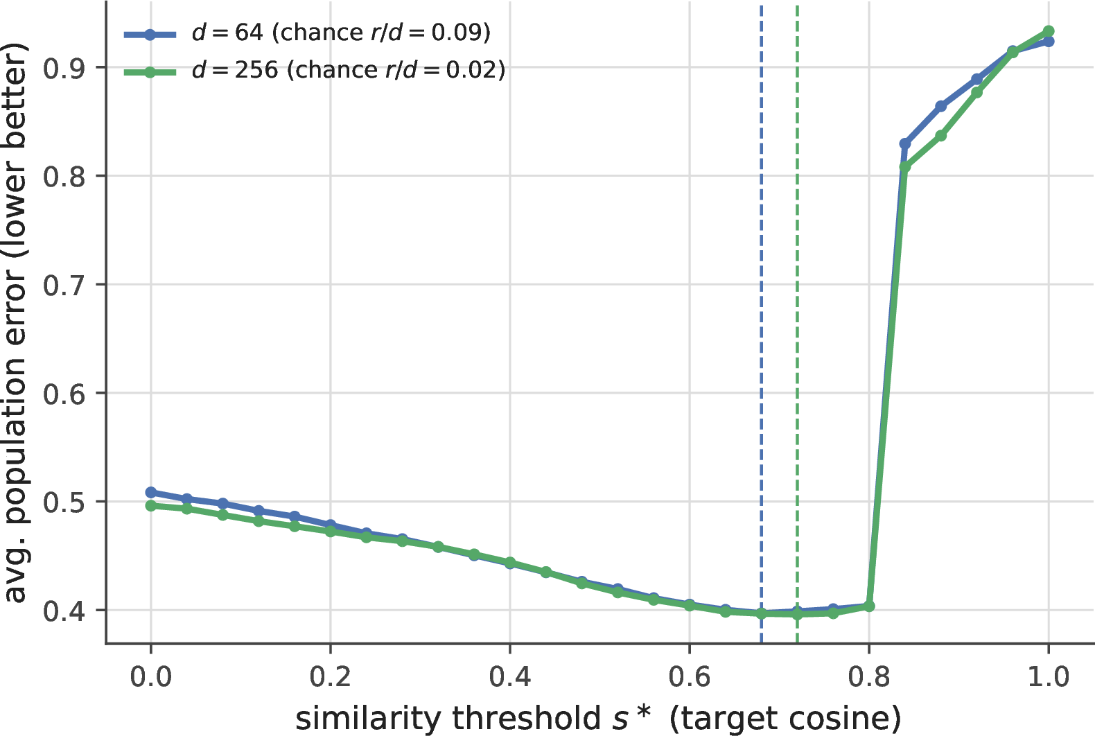
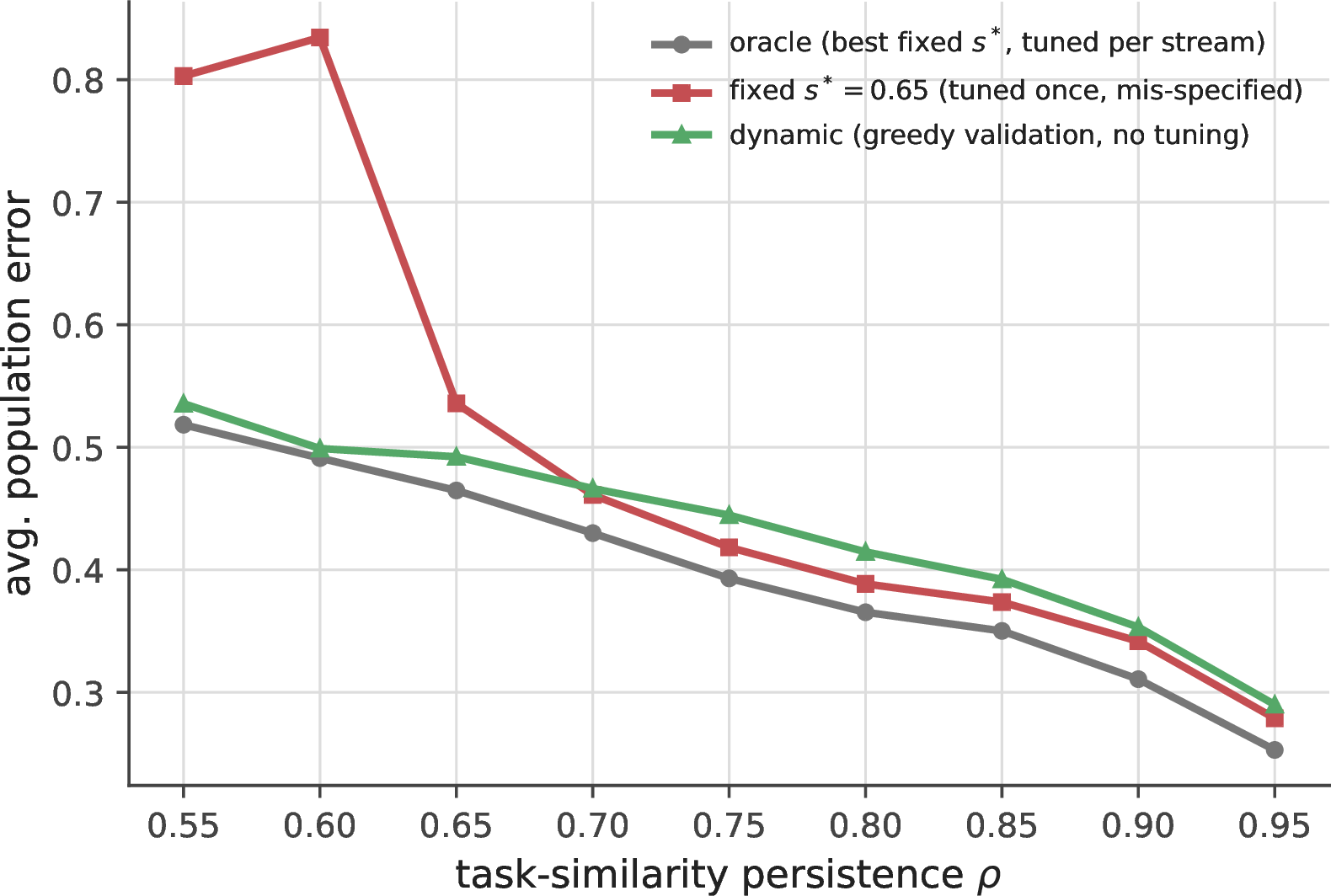
Figure 15: The similarity threshold. Left: average population error on a drifting eight-task stream versus \(s^{\ast}\), at two feature dimensions; the optimum is a broad dimension-insensitive plateau (vertical dashed lines mark each dimension’s optimum), and only \(s^{\ast}\!\to\!1\) (ogd-like isolation) is sharply suboptimal on similar tasks. Right: self-calibration removes the free parameter—the validation-greedy dynamic rule tracks the per-stream oracle within \(0.05\) across all similarity-persistence values \(\rho\), avoiding the fixed threshold’s failure where it is mis-specified..
14 Capacity limits degrade gracefully↩︎
When the rank cap \(k_{\max}\) binds, igfa overwrites the smallest-eigenvalue occupied direction. Because forgetting from removing a direction is its energy \(\tfrac12\lambda_i(u_i^\top w_A)^2\) (Theorem 1), dropping the lowest-energy direction costs the least. Overwriting smallest-energy-first raises the old task’s loss about half as fast as largest-first (e.g. \(2.0\) vs \(4.3\) at the half-way point) in a gradual degradation (Fig. 16). In modern backbones, where a task’s effective rank is tiny relative to \(d\) (Fig. 10 showed \(\approx2\) out of \(300\)), almost all overwriting hits near-zero-energy directions, so the induced forgetting is negligible.
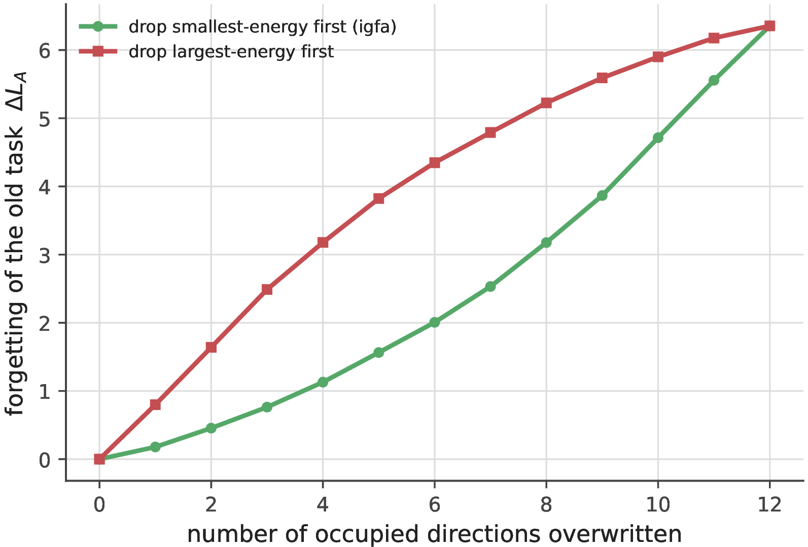
15 A pre-flight feasibility diagnostic↩︎
The distortion-floor identity (Theorem 5) bounds class-incremental accuracy by \(I(T;\phi)\); we derive from it a low-cost pre-flight test. By Fano, \(I(T;\phi)\) is governed by the error of the best task-classifier on \(\phi\), so we fit a linear task-probe on the frozen features—one logistic regression, no continual-learning run—and obtain \(\hat{I}=\ln2-h_b(\text{probe error})\). Across two-task Gaussian models of varying separation (Fig. 17), \(\hat{I}\) tracks the true \(I(T;\phi)\) at Pearson \(r=0.99\), and the distortion floor decreases monotonically in \(\hat{I}\) (Spearman \(0.97\)): the probe forecasts the floor before training. Combined with the closed-form constants of Eq. 12 , \(\hat{I}\) yields a numeric floor band, not just a ranking.
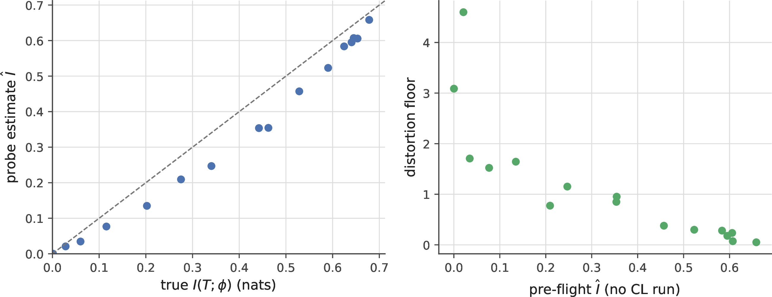
16 Low-cost online curvature: Frequent Directions↩︎
The recursive Gauss–Newton estimate used a decayed \(d\times d\) covariance and an eigendecomposition—\(\mathcal{O}(d^2)\) memory, \(\mathcal{O}(d^3)\) per task. Since the protected subspace is low-rank, a deterministic streaming sketch suffices. Replacing the full covariance with Frequent Directions [33] (an \(\ell\times d\) sketch with a bounded-error guarantee) recovers the top-\(r\) subspace almost exactly at \(\ell=2r\)—captured energy \(0.99966\) versus the full estimator’s \(0.99972\)—and beats streaming PCA (Oja, \(0.958\)) per unit memory (Fig. 18). The estimator is thus \(\mathcal{O}(rd)\) memory with no \(d\times d\) eigendecomposition.
The same holds at real scale. On a frozen pythia-160m continually pretrained with LoRA over three text domains (single run, kaggle_pending_experiments.py), the Frequent-Directions sketch captures \(0.973\) of the full-covariance energy at \(61{,}440\) floats—about \(10\times\) less than the full \(d\times d\) estimator
(\(589{,}824\) floats)—and, being a stable deterministic sketch rather than a decayed moving average, yields the lowest first-domain forgetting of the three online estimators: the domain-0 loss rises by
only \(+0.55\) then \(+0.68\) over the next two domains, versus \(+1.28\) then \(+1.58\) for the full covariance and a
diverging \(+0.33\) then \(+2.86\) for Oja streaming PCA. Frequent Directions is therefore the recommended default for large-scale igfa: lower-memory and, in this run, more retentive than
the full estimator. The full layer-wise pipeline (kaggle_H2_H3_H12.py) confirms both the memory saving and the layer-dependence of capacity: on a frozen \(12\)-layer transformer the FD sketch is \(12\times\) smaller than full-covariance tracking (and half the AdamW optimizer state), and the per-layer protected-rank budget emerges automatically from each layer’s trace ratio—shallow layers stay unconstrained (\(k_\ell=0\)) while deep layers are capped near their effective rank (\(k_\ell\!\approx\!5\)–\(7\)), with \(93\)–\(96\%\) of the deep-layer gradient routed into the protected null space and only a modest first-domain loss rise (\(+0.27\) mean).
16.0.0.1 The sketch survives drift.
The two remedies of this paper—re-estimation against drift (Sec. 5.7) and sketching against cost—compose. Under the rotating-geometry stream, a decayed Frequent-Directions sketch (\(\ell=2r\) rows, \(2rd=480\) floats at \(d=60\)) tracks the current subspace as faithfully as the full recursive covariance (\(d^2=3600\) floats): mean fidelity \(0.88\) versus \(0.85\) over ten seeds, both holding the protected rank at the true value while stale per-task protection
fills the space (evaluate_next_steps.py). Sketched curvature is a viable protected geometry under drift, not only a cheaper one.
16.0.0.2 Anchor protection: the dual construction.
The protector can also be built with no covariance at all: \(m\ge r\) stored features of the old task span \(\mathop{\mathrm{range}}\Sigma_A\) for samples in general position, so projecting updates off their orthonormalization is the eigenbasis protection. With \(d=256\) features and a \(C=400\)-output head, \(10\) anchor features give the same retention as the eigendecomposition (both at numerical zero, versus naive forgetting \(5.8\)) at a \(7\times\) cheaper construction with no \(d\times d\) covariance; the cost is independent of the output count, because the protection is a set of function-value constraints (\(W\phi_i\) fixed) living in sample space. This is the practical route for very large heads and vocabularies.
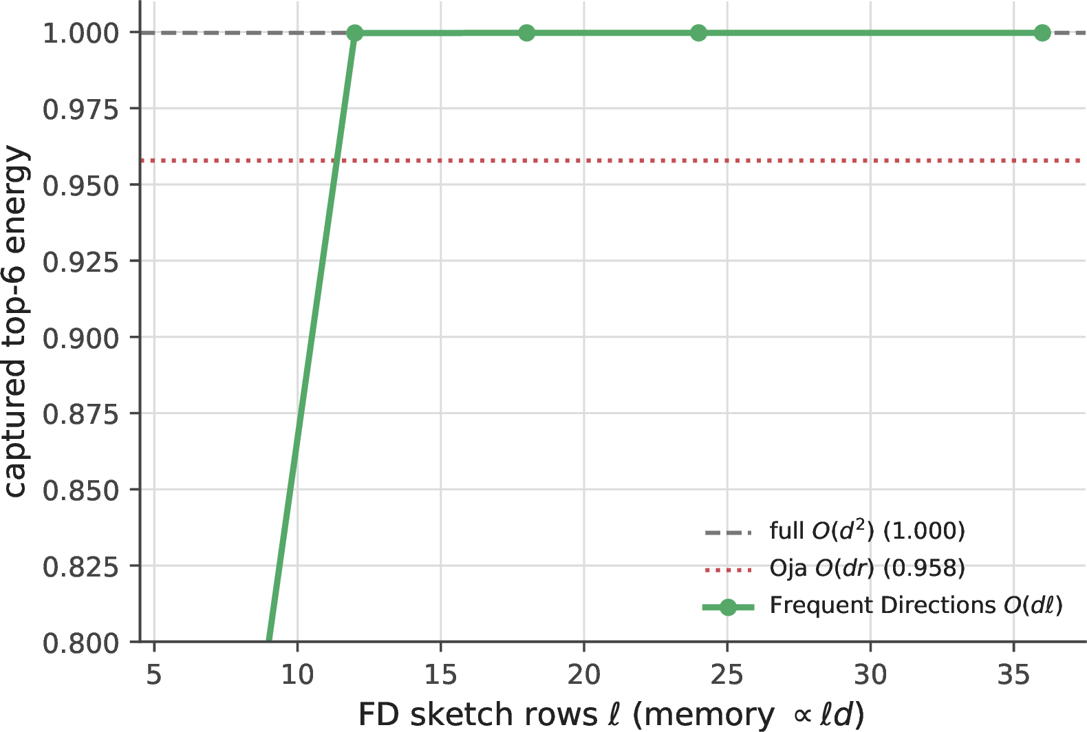
17 Soft gating and the capacity coordinate↩︎
Under the soft functional controller (keep fraction \(\mathrm{keep}_j=1/(1+\beta\lambda_j)\)) each direction is only partially protected, so capacity is consumed at rate \(\sum_j(1-\mathrm{keep}_j)\) per task. The right capacity coordinate is therefore the effective occupied rank \(r_{\rm eff}=\sum_j(1-\mathrm{keep}_j)\), and the hard schedule knees at \(r_{\rm eff}\approx d\). Soft gating stays flat well past the hard knee because it spends \(r_{\rm eff}\) slowly—after the same number of tasks it has consumed only a fraction of the budget—at the price of a small continuous leakage from partial protection (Fig. 19).
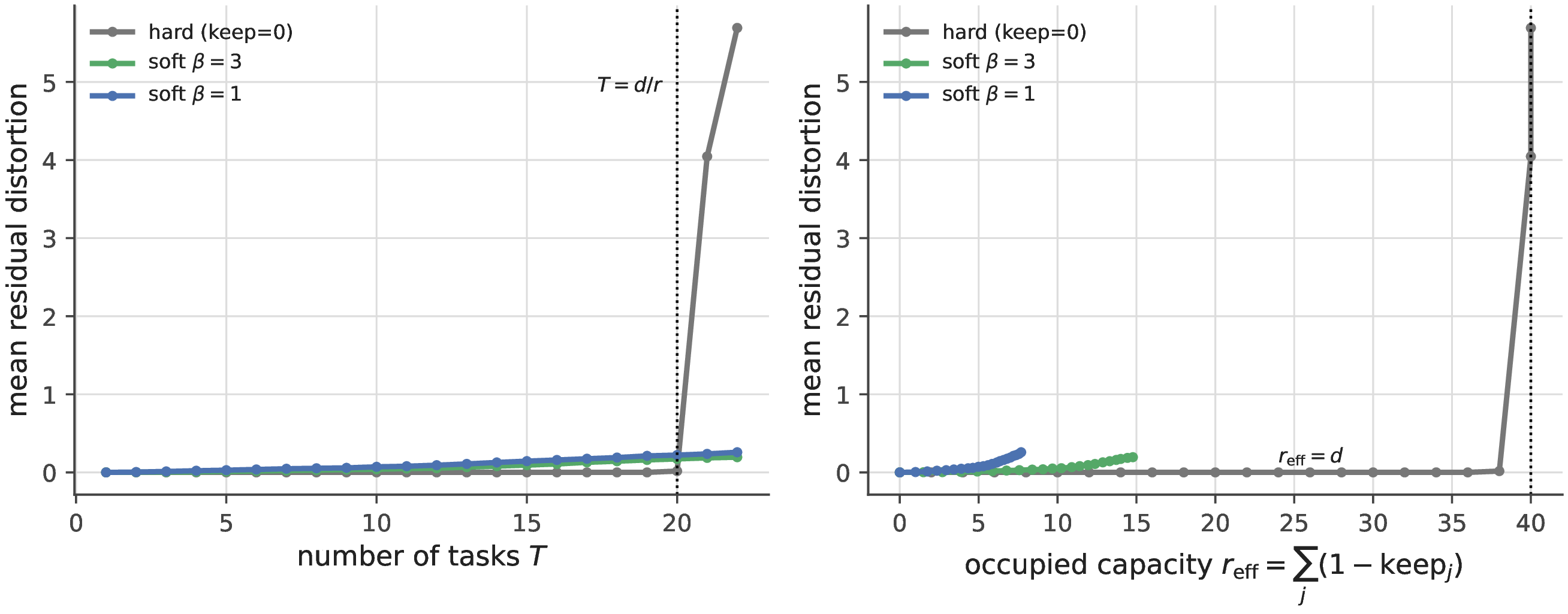
18 A per-direction gate dominates the per-task gate↩︎
The benchmark gate decides share-or-orthogonalize per task. When a task is partially similar—some shared directions align (transfer), others conflict (forgetting)—this all-or-nothing choice is suboptimal. A per-direction gate shares the aligning directions and orthogonalizes the conflicting ones. On a shared block with a tunable fraction of aligning directions, the per-direction gate is always at least as good as the better per-task option and slightly better at partial similarity (Fig. 20). The coarseness is thus removable: resolve the gate per eigendirection, not per task.
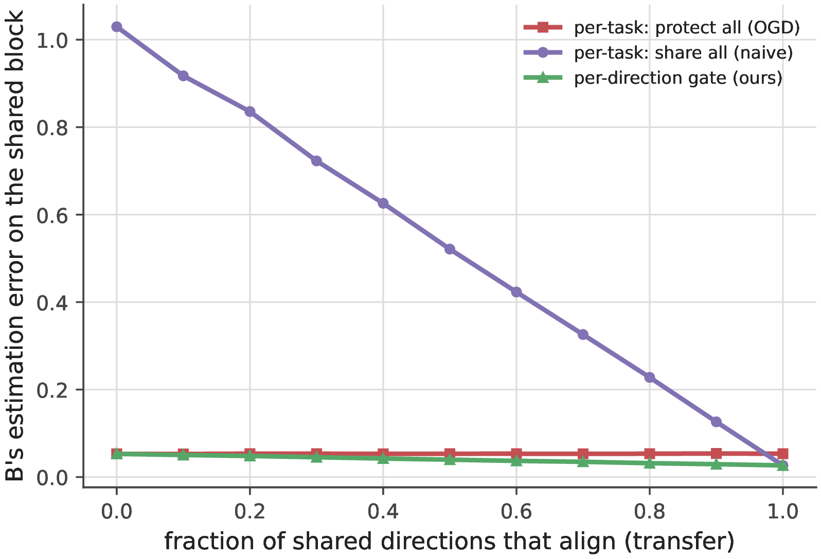
19 Billion-parameter continual pretraining↩︎
We run the three scale-sensitive pieces together on a frozen pythia-1b (\(1\)B parameters, 4-bit) with LoRA, continually pretrained on a boundary-free stream of six text domains, with the protected subspace
tracked by Frequent Directions (Sec. 16) and the pre-flight diagnostic (Sec. 15) run first. The diagnostic reports a six-way domain-probe accuracy of \(0.85\) (\(\hat{I}\approx1.52\) of a maximal \(1.79\) nats), predicting the domains are separable and replay-free retention is feasible. The run confirms it
(Table 8): the replay- and Fisher-free igfa attains both the lowest average loss (\(4.28\) vs naive \(4.54\), replay \(4.59\)) and the least first-domain forgetting after the full stream (\(+0.80\) vs naive \(+1.10\), replay \(+0.91\)), carrying
only a low-rank subspace as state. The domains are mutually dissimilar, so igfa here runs as pure structural projection. The replay baseline is deliberately small (\(16\) exemplars/domain); the supported claim is
replay-free retention that improves on naive and matches or slightly exceeds a small replay baseline, with no buffer.
| Method | Avg.final loss \(\downarrow\) | Domain-0 forgetting \(\downarrow\) | Extra state |
|---|---|---|---|
| Naive | \(4.54\) | \(+1.10\) | — |
| Replay (\(16\)/domain) | \(4.59\) | \(+0.91\) | buffer |
| (FD, replay-free) | \(\mathbf{4.28}\) | \(\mathbf{+0.80}\) | subspace |
20 Extensions and generality↩︎
The interference functional applies beyond sequential continual learning. We give eight exact-A1 proofs-of-concept on synthetic constructions (the federated, out-of-distribution, task-free, and multimodal results average over \(20\) seeds; evaluate_hypotheses.py, evaluate_applications.py, evaluate_open_questions_new.py). These are directional demonstrations of scope, not benchmarks.
To keep ambition separate from proof (Tier IV of the claim map, Sec. 6), each extension carries one of three labels. [proved-A1]: an exact consequence of the identity in the frozen-feature regime, holding wherever A1 holds—federated \(\Sigma\)-merging, the out-of-distribution projection-ratio signal, physics-informed constraints, Fisher-metric policy gradients, and floor-minimizing meta-learning. [mechanism-probe]: an empirical demonstration that the predicted mechanism operates, without a proof of optimality—task-free boundary detection, the memory-and-control instances (trust region, consolidation, floor-scheduled and dream replay), and the real-backbone results. [conjecture]: a construction whose full form needs work the paper does not complete—cross-modal \(\Sigma_{vl}\) gating and the biological floor-scheduling prediction. The label prefixes each result below.
20.0.0.1 Federated learning is \(\Sigma\)-merging.
Non-IID clients are tasks with different input geometries, and the weight divergence that FedAvg suffers coincides with the merge floor of Theorem 4. Replacing the FedAvg mean with the \(\Sigma\)-orthogonal aggregate \(w_J=(\sum_i\Sigma_i)^{+}(\sum_i\Sigma_i w_i)\), where \((\cdot)^{+}\) is the Moore–Penrose pseudo-inverse (the \(\Sigma_i\) are low-rank, so \(\sum_i\Sigma_i\) is generically singular and a plain inverse would not exist)—each client transmitting \((\Delta_i,\Sigma_i)\), or a low-rank sketch—lowers the mean client excess loss on non-IID data in every one of \(20\) seeds (mean \(1.56\times\), minimum \(1.14\times\)). Federated aggregation and continual allocation are the same \(\Sigma\)-metric optimum.
20.0.0.2 The subspace summary is a free out-of-distribution signal.
A minibatch whose gradient lies outside the occupied subspace \(U\) is structurally disjoint from the training distribution. The projection ratio \(\|UU^\top g\|/\|g\|\) is \(1.00\) for in-distribution batches and \(0.39\pm0.05\) for out-of-distribution batches (Cohen’s \(d\approx18\), minimum \(13\) across seeds), so a single threshold flags OOD inputs with no auxiliary model—an uncertainty signal obtained directly from the continual-learning state.
20.0.0.3 Fully autonomous, task-free igfa.
In a label-free stream the velocity of the recursive Gauss–Newton eigenbasis—the Frobenius commutator \(\|U_tU_t^\top U_{t-1}U_{t-1}^\top-U_{t-1}U_{t-1}^\top U_tU_t^\top\|_F\)—spikes exactly at distribution shifts, recovering randomly placed boundaries at recall and precision \(1.00\) over \(20\) streams (decay \(\gamma=0.6\)). Composing this signal with the out-of-distribution guard above removes task labels entirely: the learner declares a boundary on a velocity spike, freezes the pre-spike subspace to protect the just-finished task, skips out-of-distribution/noise batches by their orthogonal-and-extreme gradient signature, and otherwise runs the gate. On clean streams this fully autonomous igfa matches the oracle provided with the true boundaries (excess loss \(0.000\) vs \(0.000\); naive \(0.365\)); under injected extreme-magnitude OOD noise it holds at \(0.033\) while the same oracle—lacking the guard—is corrupted past \(10^{3}\), skipping \(97\%\) of noise batches at \(0.05\) false task-initializations per stream. Boundary detection, out-of-distribution rejection, and gated allocation are thus one self-regulating loop, with no human-provided task boundaries.
A velocity spike, however, presumes a sharp shift; a smoothly rotating stream never spikes. The full label-free controller therefore uses two complementary signals (evaluate_autonomous_cl.py). Novelty persistence: a batch
whose energy lies largely outside the current working subspace is held, not adapted; if the novelty persists it is a genuine task (consolidate the old task as a protected anchor, then adapt the new one), and if it subsides it was an out-of-distribution
blip (dropped)—the persistence is exactly what separates a shift from noise, since both look novel for a single batch. Working-subspace drift: a boundary is also declared when the tracked subspace rotates away from the last consolidation, which
catches gradual shifts that never spike. Consolidated anchors are capped and the closest pair \(\Sigma\)-merged when the budget is exceeded, so per-step cost is independent of stream length. Over twelve seeds against the
oracle, the controller matches it on clean shifts (detection \(F_1=1.00\), retained excess loss \(0.001\) versus \(0.001\); naive \(0.607\)), matches or beats it under noise (\(F_1=0.96\), \(0.003\) versus \(0.022\)—it skips the outliers the oracle adapts on;
naive \(0.722\)), and degrades gracefully under gradual drift (\(F_1=0.81\), \(0.274\) versus \(0.001\); naive \(0.815\)), the inherently hard case, detected with the correct latency since a smooth shift is unobservable until it accumulates. The exact-regime synthetic demonstration leaves a real unlabeled language stream open, but the
operating assumption of known boundaries is, in this regime, removed rather than merely gestured at.
20.0.0.4 Boundary-free continual learning as a memory-metric flow.
The controller above still carries thresholds (a novelty cutoff, a persistence count, a drift threshold). A differential-geometric reformulation removes them entirely, deriving autonomous operation from the geometry rather than imposing it. Drop the
notion of a task: a continuous data path \(\mathcal{D}_t\) induces an instantaneous Gauss–Newton metric \(G_t=\mathbb{E}_{x\sim\mathcal{D}_t}[\nabla f\nabla f^\top]\), accumulated into a
leaky memory metric \(\dot{M}_t=G_t-\lambda M_t\), and learning is the memory-natural-gradient flow \[\dot{\theta}=-(M_t+\varepsilon
I)^{-1}\nabla L_t.
\label{eq:memflow}\tag{13}\] Fresh directions (small \(M\)-eigenvalue) learn at rate \(\approx\!\eta\); occupied directions (eigenvalue \(s\),
i.e.past experience) are damped by \(\varepsilon/(\varepsilon+s)\), so Eq. 13 is the graded, boundary-free generalization of the projection gate, of which the hard gate \((I-QQ^\top)\) is the \(\varepsilon\!\to\!0\) spectral limit. Past losses become adiabatic invariants: for any past slice \(A\), the chain rule gives
exactly \(dL_A/dt=-\nabla L_A^\top(M_t+\varepsilon I)^{-1}\nabla L_t\), which is \(0\) when the current gradient is fresh with respect to \(A\) (\(\Sigma_t\Sigma_A=0\); verified to \(4\times
10^{-16}\)) and otherwise the interference measured in the \(M^{-1}\) inner product—the continuous form of \(\tfrac12\Delta^\top\Sigma_A\Delta\). This framing is the learning-dynamics
counterpart of energy-conserving reduced-order models on structure- preserving submanifolds [34]. Four properties are validated
(evaluate_memory_metric_flow.py). (i) On a continuously drifting stream with no boundaries, the flow drives a probe’s loss down and then holds it flat (\(0.52\!\to\!0.05\!\to\!0.08\) across
five later regimes) while naive learning loses it (\(\to0.63\)). (ii) It beats naive on gradual, sharp, and noisy streams uniformly, with no per-regime special-casing (retained loss \(0.25\)/\(0.12\)/\(0.26\) versus \(0.76\)/\(0.22\)/\(0.94\);
ten seeds), and beats hard-gating every past subspace (\(1.67\)), which over-constrains overlapping tasks the soft flow trades off. (iii) The single leak \(\lambda\) is a principled
retention–plasticity control: plasticity rises monotonically with \(\lambda\) while retention is optimized at an interior value where the memory timescale \(1/\lambda\) matches the drift
rate. (iv) A reduced-order metric (top-\(r\) eigenspace with a Woodbury inverse) reproduces the full flow at \(\mathcal{O}(dr)\) cost (\(|{\rm
diff}|=0.02\))—the structure-preserving low-dimensional submanifold carries the whole dynamics. Boundary detection, OOD rejection (a transient adds a decaying rank-one term to \(M\)), capacity (the spectrum of \(M\), released by \(\lambda\)), and gating thus collapse into one object. The flow is natural-gradient/K-FAC-shaped, but lifting it to a deep network as a running Kronecker-factored
preconditioner fails (kaggle_memory_flow_deepnet.py; 10-task Split-CIFAR-100, single seed). Swept over \(\varepsilon\in\{0.3,1,3,10\}\), the preconditioned flow either freezes after the first task or
forgets like naive and never protects a past task, reaching \(0.19\) average accuracy at best against \(0.25\) for a plain EWC penalty (naive \(0.15\)); EWC
alone holds old-task accuracy above the chance floor. The obstruction is geometric: the top Kronecker directions carry \(\approx\!99\%\) of each layer’s factor trace and coincide with the shared low-level features, so the
occupied subspace is the trunk that every later task reuses, and damping it removes plasticity instead of isolating interference. A preconditioner on a shared metric cannot separate the two; reaching depth needs a penalty formulation (the memory
metric as \(F\)) or genuinely task-specific subspaces.
20.0.0.5 Plasticity preservation: gating meets dynamical isometry.
Interference gating decides where an update may act but does not keep the allowed directions learnable: under sustained non-stationarity a network also loses plasticity as its layer Jacobians drift from isometry and the empirical NTK
grows anisotropic [35]. The failures are complementary, and pairing igfa with a dynamical-isometry regularizer—driving each weight
matrix toward orthogonality, \(R_{\mathrm{iso}}(W)=\|W^\top W-I\|_F^2\) (closed-form gradient \(4W(W^\top W-I)\), no SVD), as a decoupled AdamO step [35]—is super-additive. On a \(20\)-task Split-CIFAR-100 stream with a deeper unnormalized ReLU network
(orthogonal init, task-IL masking; three seeds; kaggle_isometry_igfa_hybrid.py), isometry alone adds \(+0.033\) average accuracy over naive and the gate alone \(+0.071\), but
together they reach \(0.555\pm0.034\) against a \(0.331\) additive prediction—a synergy of \(+0.224\), and \(2.4\times\)
naive. The gate supplies retention (old-task accuracy \(\sim\!0.5\) versus naive’s \(\sim\!0.15\)) at preserved learning while isometry supplies plasticity (learning \(0.78\), drift pinned, dead ReLUs revived); the result replicates on a harder per-task pixel-permuted stream (\(0.425\pm0.011\) versus naive \(0.215\)), with the
same ordering. Two mechanisms account for it. The gate must carry the correct sign—it acts only when a step would raise a past loss (\(\langle g,g_A\rangle<0\)) and passes beneficial transfer (\(\langle g,g_A\rangle>0\)), firing on the genuine-conflict minority of steps rather than stripping the shared learning signal that dominates a shared-feature network. And isometry makes gating cheap: the per-step
cost \(\|g-\tilde{g}\|/\|g\|\), the fraction of the gradient the projection removes, falls \(39\)–\(43\%\) once isometry is added—consistently across
mixed-aggregate (A-GEM) and per-task (GEM) gates and both streams—because in the high-rank isometric representation the conflicting component is a smaller share of the update, so protecting the past costs less of the present. A corollary: the sharper
per-task gate requires isometry, since alone it collapses the representation to rank \(\sim\!1\) and underperforms the aggregate gate, but with isometry holding effective rank high (\(25\) versus \(5.6\)) it becomes the strongest protector. The claim is comparative—absolute accuracies are low for a small unnormalized network on hard task-IL—but the ordering and the cost
mechanism are stable across three seeds and two streams.
20.0.0.6 Multimodal interference is block-structured.
For a joint embedding \(\phi=[\phi_v,\phi_l]\), the second moment \(\Sigma_A\) partitions into intra-modal blocks \(\Sigma_v,\Sigma_l\) and a cross-modal block \(\Sigma_{vl}\), and the interference energy \(\tfrac12\Delta^\top\Sigma_A\Delta\) distributes linearly across them. The cross-modal (alignment) interference of a fixed update scales with the off-diagonal \(\|\Sigma_{vl}\|\)—negligible when the modalities are unaligned and dominant when they are (energy ratio \(\gg1\) across all seeds) —so catastrophic decoupling is carried strictly by \(\Sigma_{vl}\). A cross-modal igfa would \(\Sigma_{vl}\)-orthogonalize the alignment directions while sharing the intra-modal ones. This is a synthetic decomposition; a real multimodal encoder is needed to make it conclusive.
20.0.0.7 The functional governs physics-informed constraints.
A differential constraint is a further quadratic form in feature space. For a physics-informed network with frozen features \(\phi\), the PDE residual acts on \(\phi''\), so the physics second moment is \(\Sigma_{\mathrm{PDE}}=\mathbb{E}[\phi''\phi''^\top]\) and a data-only update \(\Delta\) raises the physics loss by exactly \(\nabla L_{\mathrm{PDE}}^\top\Delta+\tfrac12\Delta^\top\Sigma_{\mathrm{PDE}}\Delta\). On a \(1\)D Poisson problem (sine random-feature basis) the interference energy \(\tfrac12\Delta^\top\Sigma_{\mathrm{PDE}}\Delta\) alone predicts the measured spike in the PDE residual at \(r=0.997\), and the full identity to machine precision (\(r=1.00000\), relative error \(2\times10^{-15}\); Fig. 21a): the functional quantifies how empirical data corrupt a physical prior, with the only change being \(\phi\mapsto\phi''\). Projecting the data gradient off the leading physics directions reduces the induced violation (\(3\times\) here) but cannot eliminate it when \(\Sigma_{\mathrm{PDE}}\) is full rank—an instance of the distortion floor of Theorem 5 under a shared active subspace.
20.0.0.8 Policy-gradient interference is governed by the Fisher.
For a linear-Gaussian policy \(\pi(a\mid s)=\mathcal{N}(\theta^\top s,\sigma^2)\) under reward \(-(a-w^\top s)^2\) the expected return is \(J(\theta)=-(\theta-w)^\top F(\theta-w)-\sigma^2\) with \(F=\mathbb{E}[ss^\top]\) the empirical Fisher: the \(\Sigma\) of supervised interference is replaced verbatim by \(F\). Across two control environments sharing a three-dimensional state subspace, routing the policy gradient orthogonal to the old-environment Fisher subspace retains the first environment perfectly (return \(0.000\) vs naive \(-10.9\); a Fisher-weighted anchor, the EWC analogue, reaches \(-1.5\); Fig. 21b) while solving the second in its free directions. The removability dichotomy of Corollary 1 holds unchanged in reinforcement learning; only the metric’s estimator changes. This is the noise-free expected gradient—a stochastic PPO/MuJoCo test is left to future work.
20.0.0.9 The distortion floor can be trained away.
Theorem 5’s floor vanishes when task second moments are mutually orthogonal, a property a feature map can be optimised to enforce. Adding the penalty \(\sum_{A<B}\operatorname{Tr}(\Sigma_A\Sigma_B)\) to a shared encoder drives its per-task subspaces apart: on overlapping synthetic tasks it cuts mean inter-task overlap \(10.6\times\) (\(0.27\to0.03\)) and the floor proxy \(\operatorname{Tr}(\Sigma_A\Sigma_B)\) by over three orders of magnitude (\(3.7\to10^{-3}\); Fig. 21c), leaving igfa to operate in the disjoint, lossless regime of Corollary 1. Structural allocation and representation learning are thus complementary: a backbone meta-trained for feature orthogonality removes the need for gating, so representation learning and structural allocation address the same distortion floor.
20.0.0.10 Certified unlearning is the dichotomy inverted.
Removability read backwards is a geometric feasibility criterion. Projecting a trained model’s update off \(\mathop{\mathrm{range}}\Sigma_F\) of a forget set removes that set’s influence exactly when forget and retain
supports are disjoint: held-out forget-set loss rises to the untrained level while retain-set performance is untouched. When the supports share \(k\) directions the removal is necessarily lossy, and the collateral damage to
the retain set is not merely bounded but predicted exactly by the retain energy on the shared support (correlation \(1.00\), zero mean error, \(44\) seeds, \(k=0\)–\(3\)): the same floor that lower-bounds forgetting lower-bounds the retain cost of exact unlearning. Support overlap is thus a principled impossibility boundary for machine unlearning
under shared representations. The two regimes separate identically on the paper’s own real benchmarks (evaluate_unlearning_real.py): on near-disjoint Split-Digits, one projection matches retraining without the forgotten task on both
sets (retained accuracy \(0.991\) versus retrain \(0.993\); the forgotten task falls to the retrain level), while on Rotated-Digits (overlap \(\approx0.68\))
the same projection necessarily damages retained rotations (\(+0.37\) mean accuracy loss versus retrain)—certified removal where supports are disjoint, the floor where they are not.
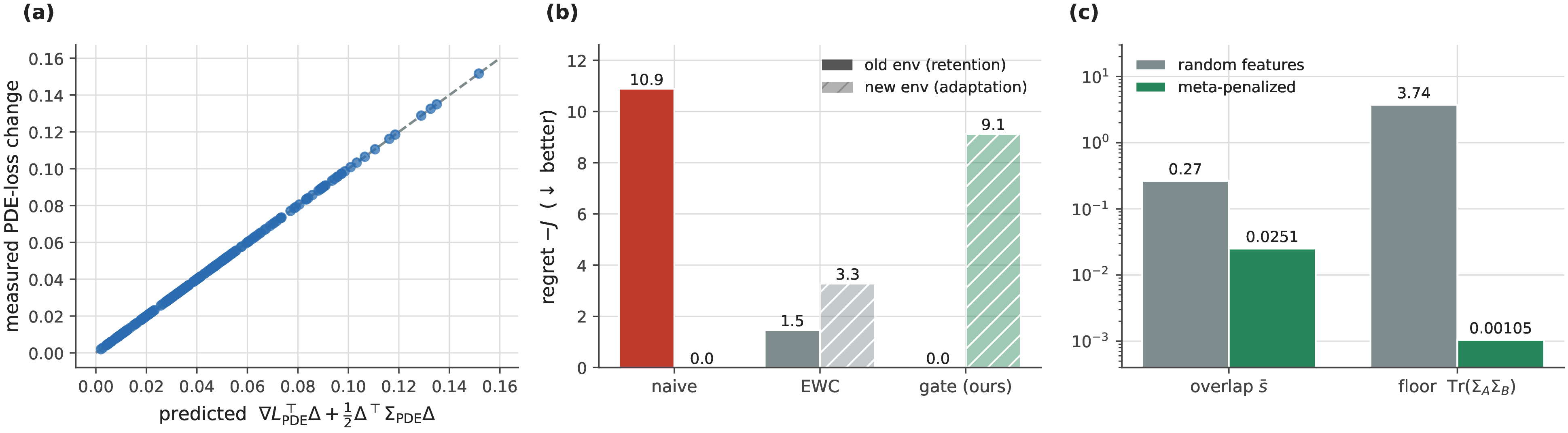
21 Memory systems and control from the functional↩︎
Beyond deciding where updates may act, the functional prescribes how much to move and when memory is worth spending. Four exact-regime demonstrations (multi-seed means; evaluate_next_steps.py) make this
operational. The framing follows complementary-learning-systems theory: a fast memory system supplies rehearsal, and the geometry decides when to invoke it.
21.0.0.1 The functional is a trust region.
Constraining each update by its predicted interference, \(\tfrac12(w-w_A)^\top\Sigma_A(w-w_A)\le B\)—equivalently, descending \(L_B+\mu\,\tfrac12(w-w_A)^\top\Sigma_A(w-w_A)\)—traces a
strictly better retention–plasticity frontier than generic step-size or early-stopping control: \(31\)–\(59\%\) lower deferred new-task loss at matched forgetting across budget levels, with
plain online gradient descent on the penalty matching the closed-form optimum. The gate of Sec. 4 is the \(\mu\to\infty\) limit of this controller on the conflicting subspace; intermediate
budgets interpolate continuously between naive descent and full protection. The controller’s metric can also be sketched: at sketch size \(\ell\ge2r\) the Frequent-Directions metric reproduces the full-covariance frontier
to \(1.3\pm0.5\%\) at \(3.6\times\) less memory, while \(\ell=r\) fails outright (\(43\%\) gap)—the same \(\ell=2r\) sizing rule as Sec. 16. At language-model scale, however, the advantage does not persist in this form: on a four-domain sequential LoRA stream with real measured forgetting, a
frozen-sketch penalty and tuned Adam schedules trace statistically indistinguishable frontiers (\(\pm0.2\%\) at matched forgetting, two seeds), with the schedule Pareto-dominant at the low-forgetting end
(kaggle_interference_optimizer.py). This is the stale-metric failure mode of Sec. 5.7 in optimizer form—frozen geometry barely helps under joint training—and it points to the current-signal controller (the
functional gate below and in Sec. 12) as the version predicted to survive scale, a prediction the functional gate then confirmed on the same stream. Under gradient noise, the residual risk of protection itself obeys a verified
diffusion law: with basis error at principal angle \(\epsilon\), the noise-driven forgetting is \(\tfrac12\eta^2\sigma^2 t\,r\sin^2\epsilon\) (measured-to-law ratio \(1.05\)–\(1.07\) across \(\eta\) and \(\epsilon\); exactly zero at \(\epsilon=0\)), which
inverts to a retention-aware step-size bound \(\eta^\ast=\sqrt{2\tau/(\sigma^2 T r\sin^2\epsilon)}\) for tolerance \(\tau\) over horizon \(T\)
(evaluate_upgrades.py).
21.0.0.2 Consolidation is spectral compression with a proven price.
When tasks share structure, the per-task protect bases are redundant. Consolidating them onto the joint spectrum—eigenvectors of the accumulated second moment at fixed captured energy— compressed the protect set by \(55\%\) (\(24\to11\) stored directions) while an adversarially conflicting new task induced at most \(0.004\) forgetting on the old family, within the dropped-eigenvalue bound of \(0.04\) that Theorem 1 supplies in advance. Offline consolidation (“sleep”) is spectral compression whose cost the theory prices before it is paid.
21.0.0.3 Memory is worth spending where the floor is positive.
With a fixed total replay budget over a stream of mixed tasks, allocating exemplars in proportion to each task’s predicted distortion floor (from \(\Sigma\)-overlap and target disagreement) retained the anchor
task \(28\pm31\%\) better than a uniform budget, improving in \(18\) of \(20\) seeds. Structural allocation handles the disjoint tasks for free, and memory
concentrates where the geometry says forgetting is otherwise unavoidable: the fast system supplies rehearsal, the functional decides when it is needed. The floor sharpens this principle into an exact policy. Full rehearsal converges to the joint optimum,
which lands every task precisely at its floor share and never below it (verified to \(3\times10^{-17}\); evaluate_replay_policy.py): rehearsal cannot buy back the floor, so the value of
replaying task \(t\) is its recoverable excess \(L_t-\mathcal{D}^\star_t\), and the optimal fixed-budget allocation is the fractional knapsack—greedy in recoverable excess per exemplar
(matches the enumerated optimum in \(20\) of \(20\) random instances). Floor-proportional allocation is the valid proxy when damage scales with conflict, the regime of the
experiment above; it misallocates in two identifiable regimes—a task already at its floor has zero replay value however large that floor, and a zero-floor task damaged by capacity coupling is fully recoverable despite its floor—where it drops below even a
uniform budget (\(3.56\) versus \(2.71\); optimum \(2.17\)). All three quantities in the policy—damage, floor, cost—are pre-flight measurables of the
ledger.
21.0.0.4 The subspace state is a replay generator.
In the exact regime, the state igfa already carries—the basis \(U\), its eigenvalues, and a weight snapshot—is a sufficient statistic for replay: sampling \(\hat{x}=U\Lambda^{1/2}z\) with
labels from the snapshot and rehearsing on these “dreamed” pairs reduces the floor exactly as real replay does (mean forgetting \(1.71\) versus \(1.72\); seedwise agreement \(r=0.97\)) with zero stored examples. The construction extends to rollouts: dreamed trajectories from a learned world model rehearse the old task nearly as well as real experience (\(2.02\) versus \(1.90\) forgetting, against \(4.23\) without replay) and degrade gracefully with model error (\(2.48\) at \(20\%\) dynamics noise), so counterfactual replay inherits the floor reduction up to the world model’s own fidelity. Replay and structural allocation are therefore not opposing families: the same low-rank state implements both,
and buffer-free generative rehearsal inherits replay’s floor reduction at sharply reduced exposure. The privacy claim can be made formal: the state is a covariance release, so the analytic Gaussian mechanism applies directly; with \(n=600\) samples behind the release, calibrated noise at \((\epsilon{=}8,\delta{=}10^{-5})\) leaves the released subspace at fidelity \(0.99\) with a
likelihood-ratio membership attack at chance, while at small \(n\) the sensitivity \(2/n\) makes certified privacy and utility incompatible (evaluate_upgrades.py)—differentially
private dream replay is viable exactly for data-rich tasks.
22 Beyond frozen features: the function-space formalism↩︎
Assumption A1 confines the exact parameter-space results to frozen features, PEFT, and first-order NTK settings. The formalism itself does not end there: recast in function space, the identity, the dichotomy, the floor, and the retention
guarantee all survive with A1 removed. Three results follow, each exact for arbitrary architectures, with validations on jointly trained deep networks (evaluate_beyond_a1.py).
22.0.0.1 The interference identity is exact in function space.
For any predictor \(f\) let \(L_A(f)=\tfrac12\,\mathbb{E}_{D_A}(f(x)-y)^2\), and let \(f_A,f_B\) be the functions realized before and after learning \(B\), by any architecture and any training procedure. Writing \(\Delta\!f=f_B-f_A\) and \(r_A=f_A-y\), expanding the square gives the identity \[\Delta L_A\;=\;\mathbb{E}_{D_A}\!\big[\Delta\!f\;r_A\big]\;+\;\tfrac12\, \mathbb{E}_{D_A}\!\big[\Delta\!f^{\,2}\big]. \label{eq:funcspace}\tag{14}\] If \(A\) is realizable and trained to convergence (\(r_A=0\) \(D_A\)-a.s.), forgetting is the function-space interference energy \(\tfrac12\|\Delta\!f\|^2_{L^2(D_A)}\): the metric is the data distribution itself, and Theorem 1 is the linear shadow of Eq. 14 (under A1, \(\Delta\!f=\Delta^\top\phi\) recovers \(\tfrac12\Delta^\top\Sigma_A\Delta\)). Numerically, Eq. 14 holds to machine precision on jointly trained depth-\(1\)–\(3\) networks (maximum relative error \(2\times10^{-7}\), \(r=1.000000\)), including the depth-\(3\) regime where the frozen-curvature predictor of Sec. 5.4 degrades to \(r\approx0.4\). Exact prediction beyond A1 costs two forward passes on \(A\)-data—no Hessian and no path integral; the parameter-space results contribute the structure, and A1 is the regime where the two pictures coincide.
22.0.0.2 The dichotomy and the floor survive, with input support in place of feature support.
Learning \(B\) is lossless for \(A\) iff \(\Delta\!f=0\) on \(\mathrm{supp}\,D_A\). For a universal model class this is achievable whenever the input supports are disjoint, at any depth; and when they overlap with disagreeing targets, the floor is a property of the data alone: minimizing pointwise, \[\min_f\;L_A(f)+L_B(f)\;=\;\tfrac12\!\int\! \frac{p_A(x)\,p_B(x)}{p_A(x)+p_B(x)}\,\big(y_A(x)-y_B(x)\big)^2\,dx, \label{eq:funcfloor}\tag{15}\] the density-overlap harmonic mean weighted by the squared target disagreement—the input-space form of Theorem 5, and a lower bound for every concrete architecture, whose own floor equals Eq. 15 plus an approximation-class excess. Measured with held-out (population) losses, a depth-\(3\) network trained jointly on conflicting sine tasks respects the bound with a \(\approx20\%\) class excess (predicted \(0.50\), measured \(0.60\)), and near-disjoint input supports give the lossless regime at any depth (predicted \(0.001\), measured \(0.009\)).
22.0.0.3 Exact retention without A1: instantaneous null-space control.
Along any absolutely continuous training path \(\theta(t)\), \(\Delta L_A=\int\langle\nabla L_A(\theta_t),\dot{\theta}_t\rangle\,dt\) exactly, with \(\nabla L_A(\theta)=\mathbb{E}_{D_A}[\,r_A(x)\,\nabla_\theta f(x;\theta)\,]\). If the velocity stays in the kernel of the current Gauss–Newton metric, \(\dot{\theta}_t\in\ker G_A(\theta_t)\) with \(G_A(\theta)=\mathbb{E}_{D_A}[\nabla_\theta f\,\nabla_\theta f^\top]\), then \(\dot{\theta}^\top G_A\dot{\theta}=0\) forces \(\langle\nabla_\theta f(x),\dot{\theta}\rangle=0\) for \(D_A\)-almost every \(x\), hence \(\langle\nabla L_A,\dot{\theta}\rangle\equiv0\) and \(L_A\) is conserved exactly—any depth, any feature drift, no A1 and no realizability. Discrete steps of size \(\eta\) leak only the Taylor remainder \(\tfrac12\eta^2 v^\top\bar H\,v\) per step (Theorem 2), i.e.\(O(\eta)\) at fixed path length. Measured at fixed path budget on jointly trained networks, forgetting under per-step re-estimated null-space control falls \(0.134\to0.0037\to0.0004\to0.00003\) as \(\eta\) drops \(0.1\to0.003\), while a frozen protected basis plateaus near \(0.5\) (staleness bias does not vanish with \(\eta\)) and naive training forgets at \(O(1)\). Assumption A1 is thereby relocated, not removed: a constant metric makes the kernel constant, so finite steps stay in it exactly—A1 buys finite-step exactness, while the geometry, the dichotomy, the floor, and the continuous-time retention guarantee never needed it. The recursive Gauss–Newton tracker of Sec. 4 is the discretization of this exact law, with the finite-step, estimation, and capacity costs quantified in Secs. 5.7, 16, and 21.
22.0.0.4 Finite-step exactness recovered: two parameter-space routes.
Even the finite-step gap closes, by two complementary mechanisms (evaluate_beyond_a1.py). (i) Region-exactness for piecewise-linear networks. For ReLU-family models the loss is exactly quadratic in each layer’s weights
while the activation pattern on the \(A\)-support is fixed: per-layer, Theorem 1 holds at finite step size inside the activation region, and the region boundary has a closed form—for a step \(sV\) in layer weights, no activation flips while \(s<\min_{i,j}|{\rm pre}_{ij}|/|(Vx_i)_j|\), computable from the stored preactivation margins. Measured: the quadratic is exact to relative
error \(10^{-11}\) inside the region, and the certificate is conservative (breakdown observed at \(1.4\pm0.4\times\) the threshold, never meaningfully before it). Assumption A1 thus relaxes,
for ReLU networks, to a checkable per-step margin condition, and the margin joins the pre-flight/ledger family as a monitorable quantity. (ii) Retraction for any smooth architecture. Exact retention means staying on the anchor level set \(\{\theta: f(x_i;\theta)=c_i\}\), and that manifold is returnable: after each ordinary update, two Gauss–Newton corrector steps on the anchor residuals restore it. Measured on jointly trained networks, anchor-set forgetting sits
at numerical zero (\(\sim10^{-14}\)) independent of step size, where projection alone leaks \(O(\eta)\) (\(0.17\), \(0.043\), \(0.0015\) at \(\eta=0.1,0.05,0.02\)), while the new task still trains. The remaining limitation is one of coverage: exactness holds on the anchors, and
between them the held-out \(A\)-loss depends on how well the anchor set pins the function class (\(0.15\)–\(0.26\) here at \(24\) anchors). Beyond A1, retention is governed by how densely the anchors sample the function class.
22.0.0.5 Monotone-retention gating: the threshold-free gate.
The path integral also yields the gate itself, with the similarity threshold removed. Since \(dL_A/dt=\langle\nabla L_A,\dot{\theta}\rangle\), the exact, modality-free rule is a sign test: given the new task’s
update direction \(g\), if \(\langle g,\nabla L_A\rangle\ge0\) the step also descends (or preserves) \(L_A\) and is kept whole; otherwise only its component
along \(\nabla L_A\) is removed, \(g\mapsto g-\frac{\langle g,\nabla L_A\rangle}{\|\nabla L_A\|^2}\nabla L_A\). In continuous time this guarantees \(dL_A/dt\le0\)—retention is monotone—while every non-harmful component of the update, and therefore all transfer, is retained; no threshold, no input geometry, and no similarity estimate appears. The single-constraint form
recovers the projections of A-GEM [2] and the surgery of PCGrad [11] as special cases, here derived from the exact identity rather than posited; per-direction refinements in the current \(G_A\)-eigenbasis coincide with the single constraint at \(A\)’s optimum (every range-component of motion is harmful there) and differ off-optimum. In the exact regime the sign gate holds forgetting at \(0.025\) versus naive \(10.06\) under pure conflict while reaching strictly lower deferred loss than unconditional projection (\(9.08\) versus \(10.06\)), and is harmless under
alignment; on jointly trained networks it attains near-current-GN retention under conflict (\(+0.14\) versus naive \(+5.77\) and frozen projection \(+5.38\), which barely helps under drift) with better adaptation than current-GN (\(0.11\) versus \(0.15\)) at a fraction of its cost—one gradient of \(L_A\) per step, from a micro-cache, the anchor construction of Sec. 16, or the dream state of Sec. 21 (evaluate_functional_gate.py). On real text
it significantly beats naive continual fine-tuning on both axes, threshold-free and without input geometry, and edges unconditional protection (Sec. 12).
The gate is, moreover, not merely a safe modification of the update but the optimal one.
Corollary 2 (The sign gate is optimal monotone control). Let \(u\) be the desired update and let tasks \(1,\dots,m\) be protected. The problem \[v^\ast=\operatorname{argmin}_v \tfrac12\|v-u\|^2 \quad\text{s.t.}\quad \langle\nabla L_{A_i},v\rangle\le 0,\;\; i=1,\dots,m, \label{eq:qpgate}\tag{16}\] has the solution \(v^\ast=u-G\lambda^\ast\) with \(G=[\nabla L_{A_1}\cdots\nabla L_{A_m}]\) and \(\lambda^\ast=\operatorname{argmin}_{\lambda\ge0}\|G\lambda-u\|\) (a nonnegative least-squares problem). For \(m=1\), \(v^\ast\) is exactly the sign gate; when no constraint is violated, \(v^\ast=u\) (sharing); when all are violated, \(v^\ast\) remains feasible yet strictly less restrictive than equality projection: protected rates may be negative—the update is allowed to improve protected tasks, which projection forbids—and \(\|v^\ast-u\|\le\|v_{\mathrm{proj}}-u\|\) always.
Intuition: stationarity of the Lagrangian gives \(v=u-G\lambda\); substituting back turns the dual into the stated nonnegative least squares, whose Karush–Kuhn–Tucker conditions are precisely primal feasibility
and complementary slackness. The gate therefore interpolates between naive sharing and subspace projection through the active set. Unconditional projection hardens those inequality constraints to equalities, which in the exact regime never improves on the
gate. All statements are machine-checked (\(\|v^\ast-v_{\mathrm{gate}}\|=0\) at \(m=1\); feasibility to \(10^{-15}\); measured protected-rate decrease under
full activation; evaluate_functional_control.py).
22.0.0.6 Beyond squared loss: the Bregman family.
The function-space results are not quadratic-loss artifacts. For any canonical loss \(\ell(y,f)=\varphi(f)-y^\top f\) with \(\varphi\) convex and mean map \(\mu=\nabla\varphi\) (squared loss: \(\varphi=\tfrac12\|f\|^2\); softmax cross-entropy: \(\varphi=\mathrm{logsumexp}\), \(\mu=\mathrm{softmax}\); logistic and Poisson likewise), the definition of the Bregman divergence \(D_\varphi(b,a)=\varphi(b)-\varphi(a)-\mu(a)^\top(b-a)\) gives, exactly and for any finite
functional change, \[\Delta L_A=\mathbb{E}_{D_A}\!\big[(\mu_A-y)^\top\Delta\!f\big]
+\mathbb{E}_{D_A}\!\big[D_\varphi(f_B,f_A)\big],
\label{eq:bregman}\tag{17}\] of which Eq. 14 is the quadratic case. For cross-entropy, \(D_\varphi(f_B,f_A)=\mathrm{KL}(p_A\,\|\,p_B)\) exactly, so on a converged task (\(\mu_A=y\) on \(\mathrm{supp}\,D_A\)) forgetting is the expected Kullback–Leibler divergence between the old and new predictive distributions. Three consequences follow. (i) The
removability dichotomy is loss-free: under A1 a kernel step changes no function value on the support, hence \(\Delta L_A=0\) exactly at any finite step size for any loss (validated at \(\|\Delta W\|=10\)); for softmax the lossless set is strictly larger, since per-sample constant logit shifts are invisible. Only the closed quadratic energy formula is squared-loss-specific. (ii) The distortion
floor has a closed information-geometric form: pointwise, \(\min_q\,[\,p_A\mathrm{KL}(\pi_A\|q)+p_B\mathrm{KL}(\pi_B\|q)\,]\) is attained at the density-weighted mixture \(q^\ast=(p_A\pi_A+p_B\pi_B)/(p_A+p_B)\), giving \[\text{floor}=\!\int\!\big(p_A(x)+p_B(x)\big)\,
\mathrm{JSD}_{w(x)}\!\big(\pi_A(\cdot|x),\pi_B(\cdot|x)\big)\,dx,
\qquad w=\tfrac{p_A}{p_A+p_B},
\label{eq:jsdfloor}\tag{18}\] a weighted Jensen–Shannon divergence between the tasks’ conditionals; the quadratic floor of Theorem 4’s function-space form is its
small-divergence (Gaussian) limit, and the mixture replaces the \(\Sigma\)-weighted mean as the optimal joint predictor. For \(T\) tasks with uniform prior the floor becomes an
information identity: writing \(T\) for the task variable, \(X\) for the input, and \(Y\) for the label,
\[\mathcal{D}^\star_T=\sum_x\sum_t p_t(x)\,\mathrm{KL}\!\big(\pi_t\,\|\,\bar\pi_x\big)
=T\cdot I(T;Y\mid X)=T\,\big[H(Y\mid X)-H(Y\mid X,T)\big],
\label{eq:infofloor}\tag{19}\] the conditional mutual information between task identity and label—the exact label-entropy cost of hiding which task a sample came from. The entropy sandwich of Theorem 6 (quadratic loss) thus closes to an equality under the loss language models train, removability becomes \(Y\perp T\mid X\), and the floor is achievable, and a trained
shared softmax head converges to Eq. 19 from above with terminal gap \(6\times10^{-16}\) (evaluate_info_floor.py; identity and mixture-optimality checks at \(10^{-16}\)). Operationally, the irreducible single-model floor of an LLM domain stream is \(I(\text{domain};\text{next token}\mid\text{context})\), estimable from micro-caches as the mean
per-domain versus mixture log-likelihood ratio. (iii) The sign gate and Corollary 2 act on \(\langle g,\nabla L_A\rangle=dL_A/dt\) and
never used the quadratic form, so they are the exact monotone controller for cross-entropy as stated—the language-model gate experiments of Sec. 12 therefore run the exact controller for the loss they train, not a transferred
heuristic. All four statements are validated to machine precision (\(10^{-16}\); kernel step exactly \(0\)), with the closed-form floor checked against direct numerical minimization
(evaluate_bregman_identity.py).
22.0.0.7 The forgetting decomposition, validated.
With \(\mathcal{D}^\star_\infty\le\mathcal{D}^\star_{\mathrm{class}}\le L\) as defined in the Discussion, \[L=\underbrace{\mathcal{D}^\star_\infty}_{\text{incompatibility}}
+\underbrace{\big[\mathcal{D}^\star_{\mathrm{class}}-\mathcal{D}^\star_\infty\big]}_{\text{capacity}}
+\underbrace{\big[L-\mathcal{D}^\star_{\mathrm{class}}\big]}_{\text{control}},
\label{eq:decomposition}\tag{20}\] an identity whose content is that the three terms are separately measurable and separately treatable. Three single-regime streams land their intended term (ten seeds;
evaluate_forgetting_decomposition.py): pure conflict under full replay is all floor (\(12.39/0/0\)); input-disjoint tasks squeezed through width-\(12\) features are all capacity
(\(0/5.35/0\)); mixed tasks under naive training carry floor plus control (\(5.42/0/4.04\)). The intervention matrix attributes cleanly: widening the features \(12\to24\) removes \(100\%\) of the capacity term while no policy—naive, active-set, or full replay—moves it at all (\(6.02\) untouched by all three); upgrading
the policy cuts only the control term (\(4.65\to2.15\), floor invariant throughout). Two definitional points the construction forces into the open: capacity means representation width—the “best rank-\(r\) subspace containing the solution” notion collapses, since any single optimum spans one dimension—and, in the quadratic regime, perturbed copies of a subspace are not conflict (their soft constraints are jointly
satisfiable and the floor is exactly zero; genuine conflict requires exactly shared support, a knife-edge the cross-entropy floor does not have, being nonzero whenever conditionals disagree on overlapping support).
22.0.0.8 Benign forgetting: the anchor splits knowledge from memorization.
The interference identity is distribution-anchored, and nothing requires the anchor to be the training set. Evaluated on task \(A\)’s deployment distribution the same identity splits observed forgetting into
knowledge loss, \(\Delta L_A^{\mathrm{test}}\), and memorization loss, \(\Delta L_A^{\mathrm{train}}-\Delta L_A^{\mathrm{test}}\)—and the two can carry opposite signs. In an
overparameterized interpolation setting with label noise (ten seeds; evaluate_benign_forgetting.py), an interfering update raises train loss by \(+1.99\)—catastrophic forgetting under any train-anchored
metric—while lowering deployment loss by \(-3.37\): backward transfer through noise removal, with the sign predicted exactly by the test-anchored identity (\(8\times10^{-16}\)).
Part of what benchmarks report as catastrophic forgetting is implicit unlearning of noise. The consequence for protection is a design law: protect the function you validated, not the function you fit. A gate whose constraint gradient is anchored
on training data defends the memorized noise together with the knowledge—it blocks benign repair and pays adaptation for the privilege— whereas the held-out-anchored gate dominates it on both axes (final deployment loss of the protected task \(8.3\) versus \(22.0\); adaptation \(5.4\) versus \(7.1\)). The anchor’s own quality gates the gate: with a held-out set too
small to be validated itself (\(M=30<d\), the anchor interpolates its own noise) the advantage collapses, which is the estimation–abstention rule’s other face. The held-out micro-caches used throughout the language
experiments (Sec. 12) are therefore mandated by the theory, not merely hygienic.
22.0.0.9 Certified unlearning is one reversed row of the gate.
Engineered benign forgetting gives an unlearning method for free: ascend the forget set’s validated loss toward the never-trained reference while the monotone-retention QP of Corollary 2 holds every retained held-out anchor in place—the unified gate with a single reversed constraint. The certificate is then a measurement, \(\mathbb{E}_{\mathrm{retain}}[\mathrm{KL}(p_{\mathrm{before}}\|
p_{\mathrm{after}})]\le\epsilon\), rather than a retraining-equivalence definition. The anchor split predicts a dichotomy, validated to machine precision (evaluate_unlearning.py): memorized content (own support) is removable at
a zero floor, whereas entangled content shared with a retained task carries a closed-form unlearning floor \(\sum_{\mathrm{shared}}p_R\,\mathrm{KL}(\pi_R\|
p_{\mathrm{ref}})\)—the surgical optimum pays exactly this (agreement \(3\times10^{-7}\)), and the gate stalls at it rather than silently damaging retained knowledge. The memorized branch holds at language-model
scale. Injecting a memorized canary into joint LoRA training on pythia-410m and pythia-1b (the earlier attempt to unlearn an entire natural domain was vacuous—the adapter had added only \(\sim0.03\) nats of removable domain-specific knowledge, the pre-flight lesson again), both the gate and naive ascent remove it fully to the base-model reference, but the gate pays \(\sim
1.7\times\) less collateral damage at both scales (retained certificate \(0.101\) versus \(0.177\) at \(410\)m, \(0.024\) versus \(0.041\) at \(1\)b; the directly measured retained-loss rise, \(+0.09\) versus \(+0.18\) and \(+0.03\) versus \(+0.07\) nats, tracks the certificate). The gate finds the zero-floor path that unstructured gradient ascent misses.
22.0.0.10 Attributed forgetting at scale.
The decomposition Eq. 20 is measurable end to end on real continual pretraining, yielding forgetting curves that state which part was ever avoidable (pythia-410m and pythia-1b, LoRA
\(r{=}8\) on the four-domain stream; per-domain single-task references, joint training as the class-optimum surrogate at ranks \(\{2,8,32\}\), sequential naive and active-set arms;
kaggle_forgetting_attribution.py, kaggle_floor_certificate.py, archived results and analysis in the repository). The floor is certified, not assumed: the generative domain classifier built from the single-domain adapters
separates held-out chunks perfectly at \(410\)m (accuracy \(1.000\), cross-entropy \(0.0048\) nats/token), and since any classifier’s cross-entropy
upper-bounds \(H(T\mid X)\ge I(T;Y\mid X)\) and the floor is a property of the data, the one bound governs both models: at least \(97.1\%\) (\(410\)m,
observed forgetting \(0.164\) nats/token) and \(98.8\%\) (\(1\)b, \(0.399\)) of the measured forgetting was avoidable in
principle. The attribution, in the exact KL observable (per-token \(\mathrm{KL}\) to the single-domain anchors, netted of the measured seed-to-seed two-models baseline of \(0.028\)/\(0.020\)):
pythia-410m |
pythia-1b |
|
|---|---|---|
| net forgetting (naive) | \(0.269\) | \(0.624\) |
| net class term | \(0.161\) | \(0.249\) |
| net control term | \(0.108\) | \(0.375\) |
| control after the active-set gate | \(0.063\) (\(41\%\) removed) | \(0.249\) (\(34\%\) removed) |
| certified floor | \(\le 0.0048\) | |
Three readings. First, the class term is real (\(6\)–\(13\times\) the seed baseline) but flat in adapter rank across \(\{2,8,32\}\): within-class interference on this stream resides in the shared frozen geometry and joint optimization, not in adapter width, so expansion is not the indicated remedy—policy is, and the gate removes a third to a half of exactly the control term (cross-entropy view: naive versus gate paired \(p=0.044\) at \(410\)m, \(p=0.0018\) at \(1\)b). Second, the decomposition’s sanity anchor holds on real data: sequential training fits each domain exactly as well as single-task training (diagonal-minus-single \(+0.000\) at \(410\)m). Third, the Bregman residual of the preceding paragraph is visible at scale: \(\mathbb{E}[\mathrm{KL}]\) exceeds the cross-entropy excess by \(0.14\)–\(0.23\) nats/token because the single-domain anchors are converged on their training chunks, not on the held-out anchor. Caveats: the recipe is fixed across scales (learning rate and budget not re-tuned, so the \(410\)m\(\to\) \(1\)b growth in forgetting is a fixed-recipe comparison), joint training only upper-bounds the class optimum (the control term is conservative), and the arms carry two to three seeds.
22.0.0.11 Protection blocks autoregressive cascades at the source.
In a generative loop, a one-step corruption of the transition operator compounds over the horizon: after fine-tuning a norm-preserving recurrence on an overlapping second task, naive rollout error grows from \(0.86\) at one step to \(1.00\) (full decorrelation) at thirty. Routing the fine-tuning update through \(\ker\Sigma_A\) keeps the old task’s transition operator invariant, and the rollout error is zero at every horizon—the cascade is blocked where it starts, not corrected downstream. Output-side correction (snapping generated states back onto the old task’s subspace) removes leakage out of the subspace but cannot repair the corrupted dynamics inside it (\(0.72\to0.99\)): for autoregressive stability, where an update acts matters more than how its outputs are post-processed.
References↩︎
github.com/anthropics/jacobian-lens.arXiv:2606.09762.