GeoTrace: Geometry-Aware Trajectory Token Compression for Video Large Language Models
July 10, 2026
Abstract
Although Video Large Language Models (Video LLMs) have shown strong performance in video understanding, their efficiency is still limited by the large number of visual tokens. Existing video token compression methods typically rely on frame-wise
saliency or heuristic token merging, which can over-focus on locally salient regions and produce ambiguous fused features. To address these issues, we propose GeoTrace, a training-free spatiotemporal token compression framework that decomposes video
evidence into exact skeleton tokens and traceable residual event tokens. Specifically, Contextual Farthest-Point Anchoring (CFPA) preserves salient, context-consistent, and high-coverage skeleton tokens, while Trajectory-Constrained Residual Condensation
(TCRC) compresses residual tokens through one-to-one temporal trajectories and constrained near-manifold condensation, producing traceable event tokens with reduced ambiguity. We evaluate GeoTrace on four Video LLMs across four video understanding
benchmarks, and the results demonstrate its effectiveness and generalization across different model architectures and scenarios. On LLaVA-OneVision, with only 10% visual tokens retained, GeoTrace achieves a \(12.99\times\)
TFLOPs reduction while preserving 99.1% of the vanilla performance. Overall, GeoTrace offers a compact and traceable token representation for efficient and robust Video LLM inference. Code is available at Code.
1 Introduction↩︎
Recent advances in Video Large Language Models (Video LLMs) have substantially improved video understanding capability [1]–[7], yet their efficiency remains constrained by the length of visual token sequences. A typical Video LLM samples frames from an input video, encodes them into visual tokens, and feeds the visual tokens together with text tokens into a large language model. Unlike text, video often contributes tens of thousands of tokens. Since the attention mechanism scales quadratically with sequence length, visual tokens frequently dominate the computational cost of Video LLMs and limit their practical deployment. Visual token compression [8]–[11] is therefore a natural remedy: by removing or merging redundant visual evidence, one can shorten the input sequence while preserving the information needed for downstream tasks.
Existing token compression methods for images [9]–[14] reduce spatial redundancy within a single frame, but they do not directly address the structure of video. Video contains both spatial redundancy and temporal redundancy, and they are often tightly coupled: whether a token is redundant depends not only on its importance within one frame, but also on how it relates to other tokens across frames. Directly applying image-oriented token compression to each frame therefore risks discarding temporal evidence or retaining locally salient but globally redundant regions. These observations call for compression mechanisms designed specifically for Video LLM inputs.
Recent Video LLM compression methods [15]–[17] typically follow three stages: temporal chunking, frame-wise token selection, and subsequent spatiotemporal compression. However, this paradigm still has two critical limitations. First, frame-wise selection is often driven by [CLS] attention scores. Such criteria tend to concentrate tokens around a few salient entities, rather than capturing the skeleton semantics of the entire frame or modeling which tokens collectively support the chunk-level spatiotemporal structure as shown in 1 (a1). As a result, the retained tokens may overrepresent a few salient entities while failing to form a compact semantic skeleton for the whole video chunk. Second, after frame-wise selection, existing methods often further split the remaining tokens into anchors and non-anchors, and then either discard the non-anchor tokens or simply aggregate them into nearby anchors. However, directly discarding residual tokens loses fine-grained temporal evidence, while heuristic aggregation can produce ambiguous features that deviate from the original feature manifold and weaken semantic discriminability, as shown in 1 (b1). These limitations motivate two questions: how can we identify skeleton tokens that represent the global structure of a video, and how can we compress the remaining non-skeleton tokens into discriminative, structure-preserving event tokens?

To address these challenges, we propose GeoTrace, a training-free spatiotemporal visual token compression framework for Video LLMs. GeoTrace preserves a chunk-level semantic skeleton while compacting non-skeleton information under explicit temporal and spatial constraints. It centers on two core compression modules: Contextual Farthest-Point Anchoring (CFPA) and Trajectory-Constrained Residual Condensation (TCRC). First, CFPA selects skeleton tokens using feature coverage, token saliency, and chunk-level contextual consistency. As shown in 1 (a2), CFPA retains semantically stable and complementary cues. Second, TCRC builds high-confidence one-to-one trajectories via Hungarian matching between adjacent frames to avoid many-to-one collapse and semantic mismatch, then performs trajectory-consistent temporal pooling and balanced spatial aggregation. As shown in 1 (b2), TCRC produces compact event tokens that stay close to the original feature manifold, preserving manifold consistency between compressed and uncompressed representations. Together, skeleton tokens and event tokens form a shorter video evidence sequence that reduces redundancy while preserving semantic discriminability and the spatiotemporal structure of video chunks.
Extensive experiments are conducted on four representative Video LLMs, including LLaVA-OneVision [1], LLaVA-Video [2], Qwen2.5-VL [4], and Qwen3-VL [5], across widely used video understanding benchmarks including VideoMME [18], LongVideoBench [19], MVBench [20], and EgoSchema [21]. Notably, on LLaVA-OneVision, GeoTrace achieves a \(12.99\times\) TFLOPs reduction while preserving \(99.1\%\) of the vanilla accuracy with only \(10\%\) of visual tokens retained. Overall, these results demonstrate the effectiveness and generalizability of GeoTrace across diverse Video LLMs and video understanding scenarios.
To summarize, our main contributions are threefold:
We identify two key limitations of existing video token compression methods: biased token selection that over-focuses on locally salient regions, and residual token handling that may discard temporal evidence or produce ambiguous fused features.
We propose GeoTrace, a training-free spatiotemporal token compression framework that uses CFPA to preserve exact skeleton tokens and TCRC to condense residual evidence into traceable event tokens.
Extensive experiments across four Video LLMs and multiple video understanding benchmarks show that GeoTrace maintains near-lossless accuracy under low visual-token retention ratios and generalizes across diverse Video LLMs and video understanding scenarios.
2 Related Work↩︎
2.0.0.1 Video LLMs.
Recent progress in large language models (LLMs) [3], [22], [23] and multimodal large language models (MLLMs) [24]–[30] has driven growing interest in extending these capabilities to video understanding, leading to the rapid development of Video LLMs [1]–[5], [7], [31]–[35]. Existing Video LLMs support a wide range of tasks, such as video question answering, long-video understanding, and open-world multimodal reasoning, by encoding sampled video frames into visual tokens and feeding them together with text tokens into an LLM. They can be divided into general Video LLMs and Video LLMs with visual token compression during training time. General Video LLMs [1]–[4], [7], [35] directly process visual tokens extracted from raw video frames, typically with lightweight pooling or temporal modeling to handle spatiotemporal information. Video LLMs with visual token compression during the training-time [36]–[40] aim to reduce the number of video tokens and thereby improve scalability to longer videos. Despite these advances, complex video understanding still imposes substantial spatiotemporal demands, and visual tokens often dominate the computational and memory overhead of LLM inference, especially for long videos with extremely large token counts. Moreover, methods that improve token efficiency during training usually require additional model adaptation and considerable hardware resources. These limitations highlight the need for training-free visual token compression methods that can improve Video LLM efficiency at inference time without costly retraining, which motivates our GeoTrace framework.
2.0.0.2 Visual Token Compression.
Visual token compression has emerged as an effective approach to reduce the cost of vision-language models by shortening the visual sequence consumed by the LLM. Image-oriented methods mainly exploit spatial redundancy: ToMe [41] merges similar tokens, SparseVLM [11] performs sparse selection and recycling, FastV [9] prunes shallow-layer tokens by text relevance, and VisionZip [10] removes encoder-side redundancy by separating informative and redundant tokens. Other methods explore adaptive retention, attention scoring, informative token selection, or graph-based redundancy analysis [12], [13], [42], [43]. However, these image-oriented methods mainly target intra-frame redundancy, while videos require modeling cross-frame repetition, trajectories, event transitions, and long-range dependencies. Recent video-specific methods exploit spatiotemporal redundancy in different ways: PruneVid [15] distinguishes static and dynamic tokens, FastVID [16] employs density-based token pruning, AOT [44] builds local-global token anchors to aggregate pruned context and preserve temporal evidence, and ST-SimDiff [17] builds a spatiotemporal token graph to jointly preserve static and dynamic evidence. Still, existing methods largely rely on heuristic, attention-based, or clustering-based strategies for token retention and merging, without explicitly separating structural evidence for preservation and residual evidence for condensation. GeoTrace fills this gap via skeleton preservation and trajectory-constrained residual condensation, yielding compact, traceable, and spatiotemporally faithful visual tokens in a training-free setting.
3 Method↩︎
3.1 Overview and Setup↩︎
GeoTrace is a training-free visual-token compression method. Given frame-level visual tokens \(\mathbf{X}=\{\mathbf{x}_{t,i}\in\mathbb{R}^{d}\}_{t=1,i=1}^{T,N}\) and [CLS] attention, GeoTrace outputs a shorter visual sequence together with inherited global indices.
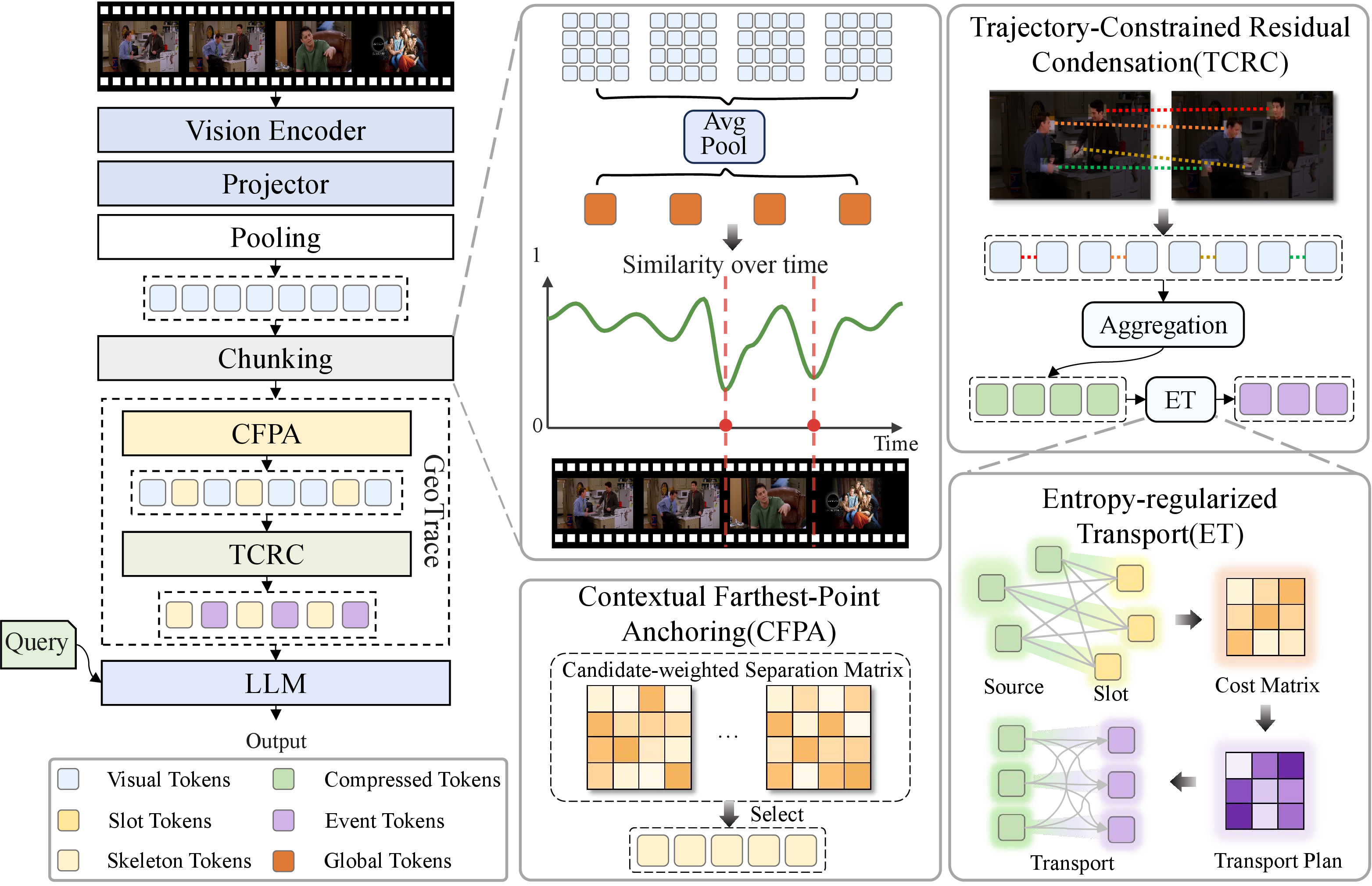
As shown in 2, GeoTrace centers on two modules: CFPA preserves exact skeleton tokens, and TCRC condenses the residual tokens into traceable event tokens. Temporal chunking defines the local scope for context estimation and trajectory matching, while global indices are used to assemble compressed tokens back in the original video order before LLM prefill.
We form temporal chunks from adjacent-frame similarity to restrict CFPA and TCRC to locally coherent intervals. For each frame, we compute a mean frame descriptor and measure the transition similarity between neighboring frames: \[\bar{\mathbf{x}}_{t} = \frac{1}{N}\sum_{i=1}^{N}\mathbf{x}_{t,i}, \qquad s_t = \cos\!\left(\bar{\mathbf{x}}_{t},\bar{\mathbf{x}}_{t+1}\right). \label{eq:main95frame95similarity}\tag{1}\] Low-similarity transitions are used as chunk cuts. This chunk-local operating scope avoids estimating context or temporal correspondences across unrelated events. Implementation details for chunk construction are provided in Appendix 8.1.
Within a chunk \(\mathcal{C}\), GeoTrace decomposes visual evidence as \[\mathbf{Z}_{\mathcal{C}} = \underbrace{\mathcal{S}_{\mathcal{C}}}_{\text{exact skeleton}} \;\cup\; \underbrace{\Phi(\mathcal{R}_{\mathcal{C}})}_{\text{traceable residual events}}, \qquad \mathcal{R}_{\mathcal{C}} = \mathbf{X}_{\mathcal{C}}\setminus\mathcal{S}_{\mathcal{C}} . \label{eq:main95factorization}\tag{2}\] Here \(\mathcal{S}_{\mathcal{C}}\) denotes the skeleton tokens selected by CFPA, \(\mathcal{R}_{\mathcal{C}}\) denotes the non-skeleton residual tokens, and \(\Phi(\cdot)\) denotes the TCRC residual condensation operator.
3.2 Contextual Farthest-Point Anchoring↩︎
Video frames often contain a set of stable objects, layout cues, and event-relevant regions that form the semantic skeleton. However, saliency-only selection tends to concentrate on a few prominent regions, context-only selection may overlook locally important visual evidence, and coverage-only selection may preserve visually dispersed noise. To preserve this skeleton without corrupting the original visual evidence, we propose CFPA. CFPA selects exact skeleton tokens that are simultaneously salient, context-consistent, and high-coverage.
CFPA first obtains a saliency matrix \(\mathbf{A}_{\mathcal{C}}\in\mathbb{R}^{|\mathcal{C}|\times N}\), which records the saliency scores of all visual tokens in each frame of the chunk. When the visual encoder exposes [CLS] attention, we construct the saliency matrix directly from the head-averaged [CLS] attention. For encoders without an explicit [CLS] token (e.g., SigLIP [45]), we derive token saliency from the visual self-attention matrix: \[\mathbf{H}_{t} = \operatorname{Softmax} \left( \frac{\mathbf{Q}_{t}\mathbf{K}_{t}^{\top}}{\sqrt{d_h}} \right) \in\mathbb{R}^{N\times N}, \qquad A_{t,j} = \frac{1}{N}\sum_{i=1}^{N}H_{t,ij}. \label{eq:main95cls95attention}\tag{3}\] This saliency matrix captures the frame-wise importance of visual tokens within the chunk.
CFPA then estimates the context consistency of each token within the chunk: \[R_{t,j} = \frac{1}{|\mathcal{C}|} \sum_{u\in\mathcal{C}} \left\langle \mathbf{x}_{t,j},\bar{\mathbf{x}}_{u} \right\rangle . \label{eq:main95context95agreement}\tag{4}\] A higher value indicates that the token is more consistent with the local video chunk, rather than salient only within an isolated frame.
Combining feature-space coverage, saliency, and context consistency, CFPA defines a candidate-weighted separation matrix: \[\Psi^t_{ij} = \bigl(1-\cos(\mathbf{x}_{t,i},\mathbf{x}_{t,j})\bigr) \cdot A_{t,j} \cdot R_{t,j}. \label{eq:main95cfpa95score}\tag{5}\] The weighting is applied on the candidate side: a token becomes a strong skeleton candidate only if it expands feature-space coverage, has high saliency, and is consistent with the local temporal context. Thus, \(\boldsymbol{\Psi}^{t}\) is interpreted as a candidate-weighted token separation score, not as a purely metric distance.
CFPA performs a beam-style farthest-point search under \(\boldsymbol{\Psi}^{t}\). This design is conceptually inspired by farthest-point sampling in point cloud processing [46], but operates on candidate-weighted token separation rather than metric distance alone. Given a partial skeleton set \(S\), each candidate expansion \(S\cup\{v\}\) is scored by its bottleneck margin: \[m_t(v\mid S) = \min_{u\in S}\Psi^t_{uv}. \label{eq:main95cfpa95margin}\tag{6}\] Instead of committing to the single best candidate at each step, CFPA ranks all candidate expansions in the beam by this bottleneck margin and keeps a small set of high-scoring partial skeletons. Because every skeleton token is copied directly from the visual encoder output, the skeleton branch provides uncorrupted anchors for stable visual structure.
The full CFPA procedure, including saliency matrix construction, context consistency estimation, candidate-weighted separation computation, and beam-style farthest-point search, is specified in detail in Appendix 8.2.
3.3 Trajectory-Constrained Residual Condensation↩︎
After skeleton preservation, the residual tokens still contain fine-grained temporal and contextual evidence. While many are redundant across nearby frames, directly discarding them removes informative details, whereas unconstrained merging may entangle unrelated regions into ambiguous features and weaken semantic discriminability. To compact this residual evidence while preserving provenance, we propose TCRC. TCRC first constructs high-confidence one-to-one temporal trajectories and then condenses trajectory-level residual features into event tokens.
For adjacent frames \(t\) and \(t+1\) in the same chunk, TCRC first extracts the non-skeleton residual indices \(I_t\) and \(I_{t+1}\), then solves a one-to-one assignment on their cosine-similarity matrix: \[\mathcal{M}_{t+1} = \arg\max_{\mathcal{M}\in\Pi} \sum_{(i,j)\in\mathcal{M}} \cos\!\left(\mathbf{x}_{t+1,i},\mathbf{x}_{t,j}\right), \label{eq:main95tcrc95matching}\tag{7}\] where \(i\in I_{t+1}\), \(j\in I_t\), and \(\Pi\) is the set of valid bipartite matchings between the two residual-token sets. We solve this maximum-similarity assignment with Hungarian matching. A matched pair is accepted only when its similarity exceeds the effective temporal threshold. The one-to-one assignment prevents multiple residual tokens in frame \(t+1\) from matching to the same residual token in frame \(t\), while thresholding rejects weak or ambiguous temporal correspondences.
These accepted token links define temporal trajectories over residual tokens. For a trajectory \(\mathcal{T}_{\ell}\), TCRC averages the features along the trajectory: \[\tilde{\mathbf{y}}_{\ell} = \frac{1}{|\mathcal{T}_{\ell}|} \sum_{(t,i)\in\mathcal{T}_{\ell}} \mathbf{x}_{t,i}. \label{eq:main95trajectory95pooling}\tag{8}\] Tokens that are not linked to any token in the previous frame form singleton trajectories and are processed in subsequent steps. The complete temporal trajectory construction procedure is detailed in Appendix 8.3.1.
After temporal trajectory construction, frames may still contain many trajectory-level representations. Let \(Y_t=\{\mathbf{y}_{t,i}\}_{i=1}^{M_t}\) denote the set of trajectory features associated with frame \(t\), where each \(\mathbf{y}_{t,i}\) is a re-indexed trajectory feature \(\tilde{\mathbf{y}}_{\ell}\), and let \(Z_t=\{\mathbf{z}_{t,k}\}_{k=1}^{B_t}\) denote the event tokens after spatial condensation. TCRC then applies entropy-regularized transport (ET): \[P_t^{\star} = \arg\min_{P\in\mathcal{U}_t} \sum_{i,k}P_{ik}\|\mathbf{y}_{t,i}-\mathbf{z}_{t,k}\|_2^2 + \varepsilon\sum_{i,k}P_{ik}\log P_{ik}. \label{eq:main95transport95condensation}\tag{9}\] Here \(P\) denotes the transport plan, and \(\mathcal{U}_t\) is the feasible polytope with uniform source and target marginals. We solve the objective with a Sinkhorn barycenter update.
Specifically, the event tokens are updated as transport-weighted barycenters, and each condensed event token inherits the global index of the source feature with the largest transport mass: \[\mathbf{z}_{t,k} \leftarrow \frac{\sum_i P^{\star}_{t,ik}\mathbf{y}_{t,i}}{\sum_i P^{\star}_{t,ik}}, \qquad g(\mathbf{z}_{t,k}) = g\!\left( \mathbf{y}_{t,\arg\max_i P^{\star}_{t,ik}} \right). \label{eq:main95barycenter95update}\tag{10}\] Thus, every event token preserves explicit evidence: its temporal evidence comes from trajectories, while its spatial evidence is dominated by source features with transport mass. Under local feature-manifold assumptions, Appendix 9 shows that TCRC event tokens stay close to the original feature manifold, preserving semantic discriminability. The solver details are given in Appendix 8.3.2.
3.3.0.1 Output assembly.
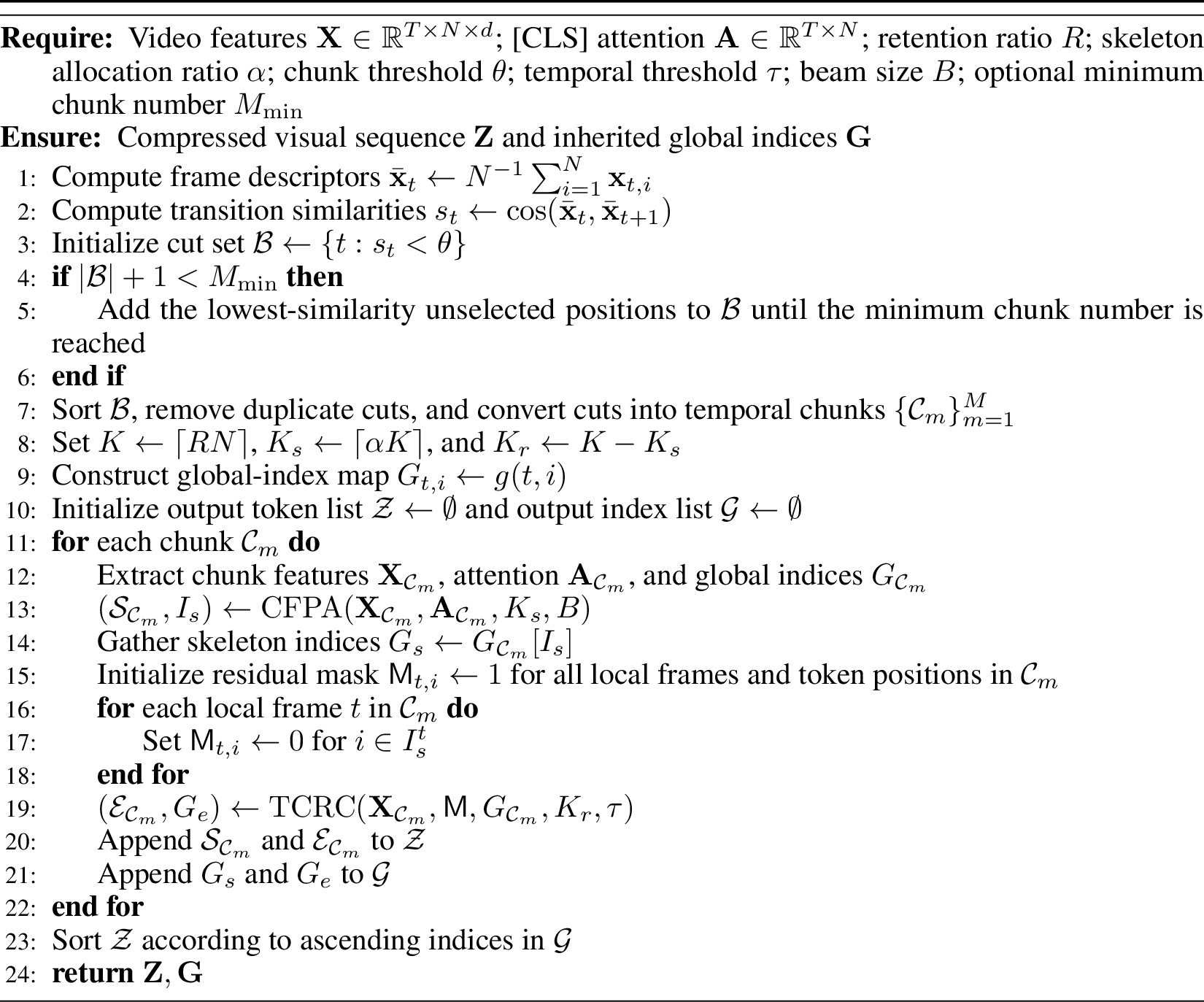
For each chunk, GeoTrace returns exact skeleton tokens from CFPA and condensed residual event tokens from TCRC, each paired with an inherited global index. We concatenate outputs from all chunks and sort them by these indices before LLM prefill. This preserves the original video order while shortening the visual sequence. The complete procedure of GeoTrace is summarized in Appendix 8.1. Complexity details are provided in Appendix 11.
4 Experiments↩︎
3.2pt
lcccccccccc & & & & & &
(lr)3-6(lr)10-11 & & Short & Medium & Long & Overall & & & & Score &
Vanilla & 100% & 69.9 & 56.7 & 48.9 & 58.5 & 60.3 & 56.6 & 58.3 & 58.4 & 100.0
FastV & & 68.1 & 54.7 & 46.8 & 56.5 & 57.8 & 55.4 & 56.4 & 56.5 & 96.7
VisionZip & & 68.8 & 57.3 & 48.2 & 58.1 & 60.4 & 56.4 & 57.8 & 58.2 & 99.7
PruneVID & & 67.3 & 54.8 & 47.2 & 56.4 & 58.1 & 55.4 & 56.8 & 56.7 & 97.1
FastVID & & 69.9 & 56.3 & 47.4 & 57.9 & 59.5 & 55.9 & 58.1 & 57.8 & 99.0
AOT & & – & – & – & 56.9 & 61.0 & 56.0 & 58.5 & 58.1 & 99.5
GeoTrace & & 70.9 & 55.8 & 49.8 & 58.8 & 60.4 & 57.1 & 58.3 & 58.7 & 100.5
FastV & & 66.3 & 53.9 & 46.9 & 55.7 & 57.6 & 56.0 & 56.0 & 56.3 & 96.4
VisionZip & & 68.6 & 57.0 & 48.3 & 58.0 & 60.0 & 55.4 & 57.6 & 57.7 & 98.8
PruneVID & & 67.2 & 53.9 & 48.2 & 56.4 & 60.2 & 55.2 & 56.2 & 57.0 & 97.6
FastVID & & 69.9 & 56.3 & 47.4 & 57.9 & 59.5 & 55.9 & 58.1 & 57.9 & 99.1
AOT & & – & – & – & 56.8 & 61.4 & 56.1 & 58.3 & 58.2 & 99.7
GeoTrace & & 70.2 & 56.7 & 47.3 & 58.1 & 60.0 & 56.3 & 58.6 & 58.3 & 99.8
FastV & & 64.6 & 54.0 & 45.3 & 54.6 & 56.6 & 54.8 & 55.0 & 55.2 & 94.5
VisionZip & & 63.8 & 54.6 & 48.3 & 55.6 & 60.0 & 54.1 & 53.5 & 55.8 & 95.5
PruneVID & & 67.2 & 52.8 & 46.7 & 56.1 & 57.7 & 54.5 & 55.1 & 55.7 & 95.4
FastVID & & 69.7 & 55.8 & 47.7 & 57.7 & 58.9 & 56.7 & 58.2 & 57.9 & 99.1
AOT & & – & – & – & 56.1 & 61.3 & 55.1 & 57.7 & 57.6 & 98.6
GeoTrace & & 68.8 & 56.2 & 47.7 & 57.6 & 59.6 & 56.8 & 57.5 & 57.9 & 99.1
FastV & & 60.9 & 52.2 & 44.9 & 52.7 & 56.0 & 52.4 & 53.4 & 53.6 & 91.8
VisionZip & & 60.3 & 52.9 & 46.7 & 53.3 & 58.5 & 49.4 & 54.8 & 54.0 & 92.5
PruneVID & & 65.9 & 52.8 & 45.6 & 54.7 & 57.2 & 54.0 & 53.7 & 54.9 & 94.0
FastVID & & 68.1 & 55.7 & 47.8 & 57.2 & 58.7 & 55.7 & 57.0 & 57.1 & 97.8
AOT & & – & – & – & 56.6 & 60.3 & 53.8 & 57.2 & 57.0 & 97.6
GeoTrace & & 67.8 & 55.4 & 48.1 & 57.1 & 60.2 & 56.6 & 57.5 & 57.9 & 99.1
Vanilla & 100% & 77.0 & 62.1 & 53.3 & 64.2 & 57.3 & 59.5 & 61.9 & 60.7 & 100.0
FastV & & 69.3 & 58.3 & 49.9 & 59.2 & 54.1 & 56.0 & 58.4 & 56.9 & 93.7
VisionZip & & 72.3 & 59.6 & 53.3 & 61.7 & 56.4 & 58.0 & 59.8 & 59.0 & 97.2
FastVID & & 74.6 & 60.8 & 52.3 & 62.6 & 55.0 & 57.1 & 60.2 & 58.7 & 96.7
ST-SimDiff & & 73.7 & 60.8 & 52.1 & 62.2 & 55.5 & 57.3 & 59.3 & 58.6 & 96.5
GeoTrace & & 73.8 & 59.7 & 51.8 & 61.7 & 56.5 & 59.0 & 60.0 & 59.3 & 97.7
FastV & & 64.3 & 53.8 & 49.2 & 55.8 & 51.1 & 53.6 & 56.2 & 54.2 & 89.3
VisionZip & & 69.4 & 57.9 & 51.2 & 59.5 & 53.9 & 54.5 & 58.5 & 56.6 & 93.2
FastVID & & 71.8 & 57.3 & 50.2 & 59.8 & 52.4 & 56.9 & 59.3 & 57.1 & 94.1
ST-SimDiff & & 71.7 & 58.7 & 50.4 & 60.5 & 54.6 & 56.8 & 58.9 & 57.7 & 95.1
GeoTrace & & 72.0 & 58.9 & 51.6 & 60.8 & 54.9 & 57.9 & 59.7 & 58.3
& 96.0
3.2pt
lcccccccccc & & & & & &
(lr)3-6(lr)10-11 & & Short & Medium & Long & Overall & & & & Score &
Vanilla & 100% & 72.6 & 61.4 & 49.9 & 61.3 & 58.3 & 58.9 & 68.0 & 61.6 & 100.0
FastV & & 69.4 & 57.0 & 51.2 & 59.2 & 57.1 & 54.2 & 66.8 & 59.3 & 96.3
VisionZip & & 69.6 & 57.2 & 50.2 & 59.0 & 56.6 & 56.3 & 66.4 & 59.6 & 96.8
FastVID & & 69.9 & 56.3 & 49.7 & 58.6 & 56.4 & 57.8 & 64.7 & 59.4 & 96.4
GeoTrace & & 69.1 & 57.1 & 48.4 & 58.2 & 57.0 & 58.6 & 67.0 & 60.2 & 97.7
FastV & & 63.7 & 54.7 & 49.3 & 55.9 & 54.9 & 51.1 & 63.6 & 57.3 & 91.6
VisionZip & & 67.0 & 54.7 & 47.6 & 56.4 & 55.5 & 54.5 & 64.3 & 57.7 & 93.7
FastVID & & 66.3 & 53.6 & 49.0 & 56.3 & 55.6 & 55.4 & 62.3 & 57.4 & 93.2
GeoTrace & & 65.4 & 55.9 & 47.3 & 56.2 & 55.4 & 57.5 & 65.5 & 58.7 & 95.3
Vanilla & 100% & 75.8 & 60.3 & 56.7 & 64.3 & 68.8 & 60.3 & 68.5 & 65.5 & 100.0
FastVID & & 69.1 & 57.0 & 53.4 & 59.9 & 66.1 & 59.8 & 63.0 & 62.2 & 95.0
AOT & & 69.3 & 56.6 & 53.9 & 59.8 & 66.1 & 58.6 & 67.0 & 62.9 & 96.0
GeoTrace & & 72.2 & 57.1 & 53.9 & 61.1 & 66.3 & 59.8 & 67.2 & 63.6
& 97.1
FastVID & & 63.7 & 60.1 & 58.6 & 60.8 & 64.0 & 58.0 & 58.6 & 60.4 & 92.2
AOT & & 62.3 & 54.8 & 55.2 & 57.8 & 63.9 & 57.1 & 62.3 & 60.3 & 92.1
GeoTrace & & 69.3 & 55.0 & 52.6 & 59.0 & 65.2 & 58.4 & 66.0 & 62.2 & 95.0
| Setting | |||||||
| Frames | |||||||
| Ratio \(R\) | VideoMME | EgoSchema | |||||
| Bench | MVBench | ||||||
| Score | |||||||
| Qwen3-VL Vanilla | 16 | 100% | 60.5 | 66.7 | 57.2 | 66.9 | 62.8 |
| Qwen3-VL + GeoTrace | 80 | 20% | 63.6 | 68.1 | 59.8 | 67.2 | 64.7 |
| Qwen3-VL + GeoTrace | 160 | 10% | 63.5 | 67.5 | 62.3 | 68.3 | 65.4 |
5.2pt
4.1 Experimental Settings↩︎
4.1.0.1 Benchmarks.
We evaluate GeoTrace on four widely used video understanding benchmarks: MVBench [20], [47], LongVideoBench [19], EgoSchema [21], and VideoMME [18]. VideoMME further reports results on its official short, medium, and long splits. Together, these benchmarks cover diverse video durations and scenarios, allowing us to assess both effectiveness and generalization.
4.1.0.2 Compared baselines.
We compare GeoTrace with six representative training-free visual token compression baselines. FastV [9] and VisionZip [10] are image-oriented methods that reduce visual tokens through attention-based pruning or encoder-side redundancy removal. PruneVid [15], FastVID [16], AOT [44], and ST-SimDiff [17] are video-oriented methods that exploit spatiotemporal redundancy through dynamic/static token selection, density-based pruning, local-global anchoring, or spatiotemporal token graphs.
4.1.0.3 Implementation details.
We evaluate GeoTrace on four Video LLMs: LLaVA-OneVision [1], LLaVA-Video [2], Qwen2.5-VL [4], and Qwen3-VL [5], covering different model architectures. Following official settings, LLaVA-OneVision and LLaVA-Video uniformly sample 32 and 64 frames, producing \(32\times196\) and \(64\times169\) visual tokens, respectively. For Qwen2.5-VL and Qwen3-VL, we uniformly sample 32 frames and keep official video-processor settings unchanged, so their visual-token counts are determined by the dynamic-resolution processor and generated video grid. For fair comparison with baselines, we match the average number of visual tokens processed per Transformer layer across methods. This layer-wise token count serves as a proxy for comparable computational cost in Video LLMs. Default hyperparameters and the detailed budget-alignment formulation are provided in Appendix 8 and 10. We conduct all evaluations using LMMs-Eval [48] on A100 GPUs.
4.2 Main Results↩︎
We evaluate GeoTrace under different retention ratios \(R\). The main paper reports all results for LLaVA-OneVision at the \(10\%\), \(15\%\), \(20\%\), and \(25\%\) retention settings, as well as the representative \(20\%\)/\(10\%\) settings for the other Video LLMs in ¿tbl:tab:llava95ov95video95results? ¿tbl:tab:qwen2595qwen395results?. Results for the other Video LLMs and compared baselines at the remaining \(25\%\) and \(15\%\) settings are provided in Appendix 6.
4.2.0.1 Results on LLaVA-OneVision.
¿tbl:tab:llava95ov95video95results? shows that GeoTrace achieves the best performance across all retention ratios \(R\). It retains \(99.1\%\) of vanilla accuracy at \(R=10\%\), while surpassing the vanilla model at \(R=25\%\). Compared with baselines, GeoTrace degrades more gracefully as the token budget shrinks. This pattern suggests that preserving skeleton evidence and compacting residual temporal evidence can remove redundant video tokens with only mild performance degradation.
4.2.0.2 Results on LLaVA-Video.
¿tbl:tab:llava95ov95video95results? further shows that GeoTrace achieves the best average score on LLaVA-Video at both \(20\%\) and \(10\%\) retention. Since LLaVA-Video samples more frames than LLaVA-OneVision, the visual sequence contains denser cross-frame redundancy and finer temporal evidence. GeoTrace is strongest at \(R=10\%\), where it outperforms all baselines on every metric. This suggests that TCRC is useful when dense video-frame sequences are compressed aggressively.
4.2.0.3 Results on Qwen2.5-VL.
¿tbl:tab:qwen2595qwen395results? shows that GeoTrace achieves the best average score and accuracy on Qwen2.5-VL at both \(20\%\) and \(10\%\). Although it is not always the best on VideoMME, it improves LongVideoBench and MVBench, which involve broader temporal and task diversity. This indicates that GeoTrace is not tied to fixed-grid LLaVA architecture. Its chunk-level skeleton selection and residual condensation remain effective under dynamic-resolution visual layouts.
4.2.0.4 Results on Qwen3-VL.
¿tbl:tab:qwen2595qwen395results? also confirms the benefit of GeoTrace on the stronger Qwen3-VL backbone. GeoTrace achieves the best average score at both \(20\%\) and \(10\%\), improving relative accuracy to \(97.1\%\) and \(95.0\%\), respectively. While FastVID remains competitive on some VideoMME scores, GeoTrace is more balanced across EgoSchema, LongVideoBench, and MVBench. These gains show that the proposed GeoTrace remains useful even with a stronger underlying VLLM.
4.2.0.5 Using GeoTrace to increase temporal coverage.
GeoTrace can also trade redundant per-frame tokens for broader temporal coverage under a matched visual-token budget. On Qwen3-VL, increasing sampled frames from 16 to 80 and 160 improves the average score from \(62.8\) to \(64.7\) and \(65.4\), respectively. The 160-frame setting is especially beneficial on LongVideoBench, where longer temporal evidence can matter. This suggests that compression is useful not only for acceleration but also for exposing the LLM to a longer temporal context.
4.3 Ablation Study↩︎
4.3.0.1 Overview.
We ablate the main design choices of GeoTrace on LLaVA-OneVision. The study examines the effectiveness of the CFPA skeleton branch and the TCRC residual branch, analyzes the skeleton allocation ratio \(\alpha\), and reports efficiency under different retention ratios.
4.3.0.2 Ablation study on CFPA module.
We ablate CFPA at \(R=10\%\) on LLaVA-OneVision. In ¿tbl:tab:cfpa95ablation?, Sal., Cons., and Cov. denote saliency-only, context-consistency-only, and coverage-only selection. The two removal variants test whether context consistency and saliency are both needed in the full CFPA score. This isolates how each component contributes to stable skeleton preservation.
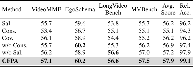
The full CFPA achieves the best average score and relative accuracy, improving the average score over Sal./Cov. by \(1.7\) and over Cons. by \(2.8\). Removing either context consistency or saliency also reduces the average score, showing that neither term is redundant. These results show that saliency, context consistency, and coverage play complementary roles: saliency identifies important evidence, context filters frame-local noise, and coverage avoids redundant local regions.
4.3.0.3 Ablation study on TCRC module.
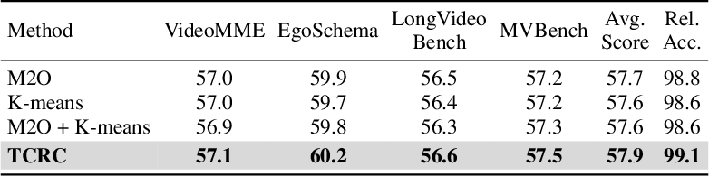
We ablate TCRC at \(R=10\%\) on LLaVA-OneVision in [tbl:tab:tcrc95ablation]. M2O replaces one-to-one temporal matching with many-to-one matching, while K-means replaces ET condensation. Both variants reduce the average score, and their combination does not recover the loss. This supports the two-part TCRC design: one-to-one temporal trajectory construction keeps residual evidence traceable, while ET condensation provides a more stable spatial summary.
4.3.0.4 Ablation study on skeleton allocation ratio \(\alpha\).
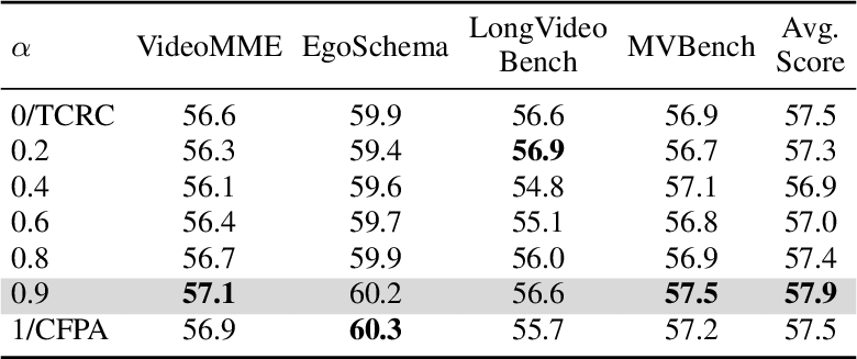
We use \(\alpha\) to allocate the retained token budget between CFPA skeleton tokens and TCRC event tokens. ¿tbl:tab:alpha95ablation? evaluates different \(\alpha\) values at \(R=10\%\) on LLaVA-OneVision. The best average score is obtained at \(\alpha=0.9\), where most of the budget preserves exact skeleton evidence while a small portion remains for residual temporal evidence. Both endpoints, \(0/\mathrm{TCRC}\) and \(1/\mathrm{CFPA}\), underperform in this mixed setting, indicating that CFPA and TCRC provide complementary benefits.
4.3.0.5 Efficiency under different retention ratios.
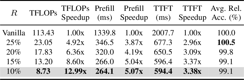
We measure efficiency on LLaVA-OneVision using VideoMME, with latency measured on an A100 GPU, as shown in [tbl:tab:efficiency95ablation]. At \(R=10\%\), GeoTrace reduces computation from \(113.43\) to \(8.73\) TFLOPs and improves TTFT from \(2007.7\) ms to \(594.4\) ms. The TTFT speedup is smaller than the TFLOPs reduction because it includes non-prefill overheads, but the end-to-end gain is still substantial. Since this setting retains \(99.1\%\) relative accuracy, the efficiency gains translate into practical acceleration rather than merely stronger pruning.
5 Conclusion↩︎
We introduced GeoTrace, a training-free visual-token compression framework for Video LLMs. GeoTrace separates video evidence into exact skeleton tokens selected by CFPA and traceable event tokens condensed by TCRC, preserving core visual structure while compacting redundant residual temporal evidence without weakening semantic discriminability. Across multiple Video LLM backbones and video understanding benchmarks, GeoTrace maintains strong accuracy under aggressive retention ratios and delivers substantial prefill and TTFT speedups. These results highlight the value of geometry-aware skeleton preservation and trajectory-constrained residual condensation for efficient video-language understanding. Future work may extend GeoTrace toward adaptive token budgeting, streaming video inference, and broader model-specific deployment settings.
Appendix
Additional VLLM Results to 0.65em.
Additional Ablation Results to 0.65em.
Supplementary Method Details to 0.65em.
GeoTrace Pipeline and Bookkeeping to 0.65em.
Contextual Farthest-Point Anchoring Details to 0.65em.
Trajectory-Constrained Residual Condensation Details to 0.65em.
Near-Manifold Preservation of TCRC to 0.65em.
Token Budget Alignment to 0.65em.
Complexity to 0.65em.
Qualitative Demonstrations to 0.65em.
Limitations to 0.65em.
6 Additional VLLM Results↩︎
3.2pt
lcccccccccc & & & & & &
(lr)3-6(lr)10-11 & & Short & Medium & Long & Overall & & & & Score &
Vanilla & 100% & 77.0 & 62.1 & 53.3 & 64.2 & 57.3 & 59.5 & 61.9 & 60.7 & 100.0
FastV & & 71.7 & 59.2 & 50.9 & 60.6 & 54.8 & 56.4 & 59.1 & 57.7 & 95.1
VisionZip & & 74.0 & 60.3 & 52.9 & 62.4 & 57.0 & 58.3 & 60.0 & 59.4 & 97.9
FastVID & & 74.7 & 60.1 & 53.6 & 62.8 & 55.4 & 58.2 & 60.5 & 59.2 & 97.5
ST-SimDiff & & 74.2 & 61.4 & 52.5 & 62.7 & 55.7 & 57.4 & 59.6 & 58.9 & 97.0
AOT & & – & – & – & 62.4 & 55.6 & 55.9 & 59.2 & 58.3 & 96.0
GeoTrace & & 74.6 & 60.0 & 51.2 & 61.9 & 56.4 & 59.5 & 59.8 & 59.4 & 97.9
FastV & & 67.9 & 56.9 & 50.8 & 58.5 & 53.1 & 54.5 & 57.5 & 55.9 & 92.1
VisionZip & & 72.9 & 58.1 & 51.9 & 61.0 & 55.7 & 57.2 & 59.6 & 58.4 & 96.2
FastVID & & 73.4 & 58.1 & 51.8 & 61.1 & 54.1 & 57.7 & 60.3 & 58.3 & 96.0
ST-SimDiff & & 73.2 & 60.1 & 51.4 & 61.5 & 55.1 & 56.9 & 59.2 & 58.2 & 95.9
AOT & & – & – & – & 61.9 & 54.8 & 54.6 & 57.7 & 57.3 & 94.4
GeoTrace & & 72.4 & 58.9 & 50.7 & 60.7 & 55.9 & 58.4 & 60.4 & 58.9 & 97.0
Vanilla & 100% & 72.6 & 61.4 & 49.9 & 61.3 & 58.3 & 58.9 & 68.0 & 61.6 & 100.0
FastV & & 71.2 & 57.8 & 51.6 & 60.2 & 57.2 & 54.6 & 67.4 & 59.8 & 97.1
VisionZip & & 70.7 & 57.9 & 51.2 & 59.9 & 57.0 & 57.1 & 67.3 & 60.3 & 97.9
FastVID & & 71.2 & 57.8 & 49.9 & 59.6 & 56.7 & 58.0 & 65.5 & 60.0 & 97.4
GeoTrace & & 71.2 & 57.9 & 49.2 & 59.4 & 57.1 & 58.7 & 67.1 & 60.6 & 98.4
FastV & & 67.4 & 55.2 & 51.1 & 57.9 & 56.5 & 52.2 & 65.9 & 58.1 & 94.3
VisionZip & & 68.8 & 56.7 & 49.1 & 58.2 & 55.7 & 56.3 & 66.0 & 59.0 & 95.8
FastVID & & 68.2 & 56.9 & 49.4 & 58.2 & 56.0 & 56.8 & 63.6 & 58.6 & 95.1
GeoTrace & & 68.6 & 55.7 & 47.8 & 57.3 & 56.3 & 57.6 & 66.3 & 59.4 & 96.4
Vanilla & 100% & 75.8 & 60.3 & 56.7 & 64.3 & 68.8 & 60.3 & 68.5 & 65.5 & 100.0
FastVID & & 71.4 & 57.9 & 53.7 & 60.3 & 64.0 & 59.6 & 64.8 & 62.2 & 95.0
AOT & & 70.8 & 57.1 & 53.7 & 60.9 & 65.8 & 59.0 & 66.8 & 63.1 & 96.3
GeoTrace & & 73.8 & 57.9 & 53.0 & 61.6 & 66.7 & 60.0 & 67.5 & 64.0 &
97.7
FastVID & & 65.0 & 56.0 & 55.3 & 59.1 & 65.0 & 58.5 & 62.1 & 61.2 & 93.4
AOT & & 64.9 & 55.6 & 56.6 & 59.0 & 65.4 & 57.9 & 64.4 & 61.7 & 94.2
GeoTrace & & 72.1 & 56.1 & 53.7 & 60.6 & 66.0 & 58.9 & 67.0 & 63.1 &
96.3
7 Additional Ablation Results↩︎
7.0.0.1 Ablation study on temporal threshold \(\tau\).
TCRC uses the temporal threshold \(\tau\) to decide whether a matched residual-token edge should be accepted into a one-to-one trajectory. A lower threshold preserves more temporal links but may admit ambiguous correspondences, while a higher threshold keeps only more confident matches but may break useful trajectories. ¿tbl:tab:tau95ablation? reports the sensitivity of GeoTrace to \(\tau\) at \(R=10\%\) on LLaVA-OneVision.

The results are stable across a broad range of thresholds, with \(\tau=0.7\) and \(\tau=0.8\) achieving the best average score. We use \(\tau=0.8\) by default because it matches the best average score while giving the strongest MVBench result and tied-best EgoSchema and LongVideoBench results. This suggests that TCRC benefits from relatively strict temporal matching, which filters weak correspondences without overly fragmenting residual trajectories.
7.0.0.2 Ablation study on CFPA beam size.
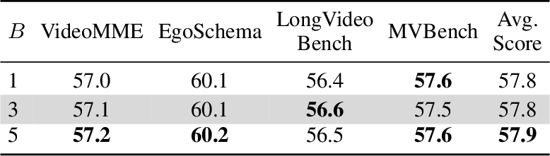
CFPA uses beam-style farthest-point search to avoid committing to a single greedy skeleton expansion at each step. [tbl:tab:beam95size95ablation] reports the effect of the beam size \(B\) at \(R=10\%\) on LLaVA-OneVision.
Increasing the beam size from \(1\) to \(3\) improves LongVideoBench and slightly improves VideoMME, showing that maintaining multiple candidate skeletons helps avoid locally suboptimal selections. A larger beam size \(B=5\) gives a marginally higher average score, but the gain over \(B=3\) is only \(0.1\) while requiring more beam expansions. We therefore use \(B=3\) as the default setting, which balances accuracy and efficiency.
8 Supplementary Method Details↩︎
This appendix provides implementation-level details omitted from the main Method section. 8.1 specifies the GeoTrace pipeline, including temporal chunk construction, budget bookkeeping, residual-mask construction, and final assembly. 8.2 gives the complete CFPA skeleton selection procedure. 8.3 describes TCRC residual condensation, with temporal trajectory construction in 8.3.1 and Sinkhorn barycenter condensation in 8.3.2.
8.0.0.1 Default hyperparameters.
Unless otherwise specified, GeoTrace uses beam size \(B=3\) for CFPA, temporal threshold \(\tau=0.8\) for TCRC, and skeleton allocation ratio \(\alpha=0.9\). These choices are supported by the ablations in ¿tbl:tab:tau95ablation? [tbl:tab:beam95size95ablation] ¿tbl:tab:alpha95ablation?: \(B=3\) provides nearly the same accuracy as a larger beam with fewer beam expansions, \(\tau=0.8\) gives the best average score while maintaining strict temporal matching, and \(\alpha=0.9\) preserves most of the budget as exact skeleton evidence while retaining a small residual-event channel. For temporal chunking, we set the minimum number of chunks to \(M_{\min}=8\), which avoids overly long chunks and keeps trajectory matching within locally coherent video intervals. For Sinkhorn barycenter condensation, we use entropy strength \(\varepsilon=0.05\) and \(L_{\mathrm{ot}}=3\) outer barycenter iterations. This small iteration count is sufficient because Sinkhorn condensation is only used after CFPA and temporal routing have already restricted the residual groups to local evidence.
Throughout this appendix, we use one-indexed notation for readability. The implementation may use zero-indexed tensors without changing the algorithm. For a token at frame \(t\) and spatial position \(i\), its global index is: \[g(t,i)=(t-1)N+i. \label{eq:app95global95index}\tag{11}\]
8.1 GeoTrace Pipeline and Bookkeeping↩︎
GeoTrace constructs temporal chunks from adjacent-frame similarities. Given visual features \(\mathbf{X}\in\mathbb{R}^{T\times N\times d}\), the frame descriptor and transition similarity are \[\bar{\mathbf{x}}_t = \frac{1}{N}\sum_{i=1}^{N}\mathbf{x}_{t,i}, \qquad s_t = \cos(\bar{\mathbf{x}}_t,\bar{\mathbf{x}}_{t+1}), \quad t=1,\ldots,T-1. \label{eq:app95transition95similarity}\tag{12}\] Positions with \(s_t<\theta\) are used as chunk boundaries. If fewer than the required number of chunks are produced, GeoTrace adds the lowest-similarity unselected transitions as complementary cuts. Zero-length chunks caused by duplicate cuts are removed.
Given retention ratio \(R\), skeleton allocation ratio \(\alpha\), and \(N\) visual tokens per frame, the per-frame budgets are \[K=\lceil RN\rceil,\qquad K_s=\lceil\alpha K\rceil,\qquad K_r=K-K_s. \label{eq:app95budget95split}\tag{13}\] For a chunk \(\mathcal{C}\), CFPA selects \(K_s\) skeleton tokens per frame. These selected positions are removed from the residual mask before TCRC is applied. 3 summarizes the complete GeoTrace pipeline.
8.2 Contextual Farthest-Point Anchoring Details↩︎
CFPA selects skeleton tokens using a candidate-weighted farthest-point objective. For a chunk with \(L\) frames, the chunk-context agreement of token \(\mathbf{x}_{t,j}\) is \[\rho_{t,j} = \frac{1}{L} \sum_{u=1}^{L} \left\langle \mathbf{x}_{t,j},\bar{\mathbf{x}}_u \right\rangle . \label{eq:app95context95agreement}\tag{14}\] Let \(a_{t,j}\) denote the [CLS] attention score of token \(j\) in frame \(t\). CFPA defines \[D^t_{ij} = 1-\cos(\mathbf{x}_{t,i},\mathbf{x}_{t,j}), \qquad \psi_t(i\rightarrow j) = D^t_{ij}\cdot a_{t,j}\cdot\rho_{t,j}. \label{eq:app95cfpa95score}\tag{15}\] In the implementation, attention scores are multiplied by a positive constant for numerical stability; this constant does not change the ranking induced by the score.
For a partial skeleton set \(S\), the farthest-point margin is: \[m_t(v\mid S) = \min_{u\in S}\psi_t(u\rightarrow v). \label{eq:app95cfpa95margin}\tag{16}\] The beam search approximates the context-aware max-min subset selection: \[I_s^t \approx \arg\max_{S\subseteq\{1,\ldots,N\},\,|S|=K_s} \min_{v\in S} \min_{u\in S\setminus\{v\}} \psi_t(u\rightarrow v). \label{eq:app95cfpa95objective}\tag{17}\] 4 gives the full selection procedure.

8.3 Trajectory-Constrained Residual Condensation Details↩︎
TCRC operates only on non-skeleton residual tokens indicated by the residual mask \(\mathsf{M}\). It first constructs high-confidence one-to-one trajectories across adjacent frames, then performs budget-balanced spatial condensation when the surviving residual roots exceed the residual-event budget.
8.3.1 Temporal Trajectory Construction↩︎
For adjacent frames \(t\) and \(t+1\), let \(I_t=\{i:\mathsf{M}_{t,i}=1\}\) and \(I_{t+1}=\{i:\mathsf{M}_{t+1,i}=1\}\). TCRC computes the residual similarity matrix \[S^{t+1}_{ab} = \cos\!\left( \mathbf{x}_{t+1,I_{t+1}[a]}, \mathbf{x}_{t,I_t[b]} \right), \label{eq:app95tcrc95similarity}\tag{18}\] and solves Hungarian matching on \(-S^{t+1}\). A matched current-frame residual token is routed to its predecessor only when the matched similarity exceeds an effective threshold \(\tau_{\mathrm{eff}}\).
The threshold starts from \(\tau\). If too many residual tokens are routed backward and the number of surviving residual roots falls below \(K_rL\), GeoTrace raises the threshold so that at most \[n_{\max} = \sum_{t,i}\mathsf{M}_{t,i} - K_rL \label{eq:app95route95bound}\tag{19}\] Residual tokens are routed. This prevents temporal condensation from exceeding the residual-event budget.
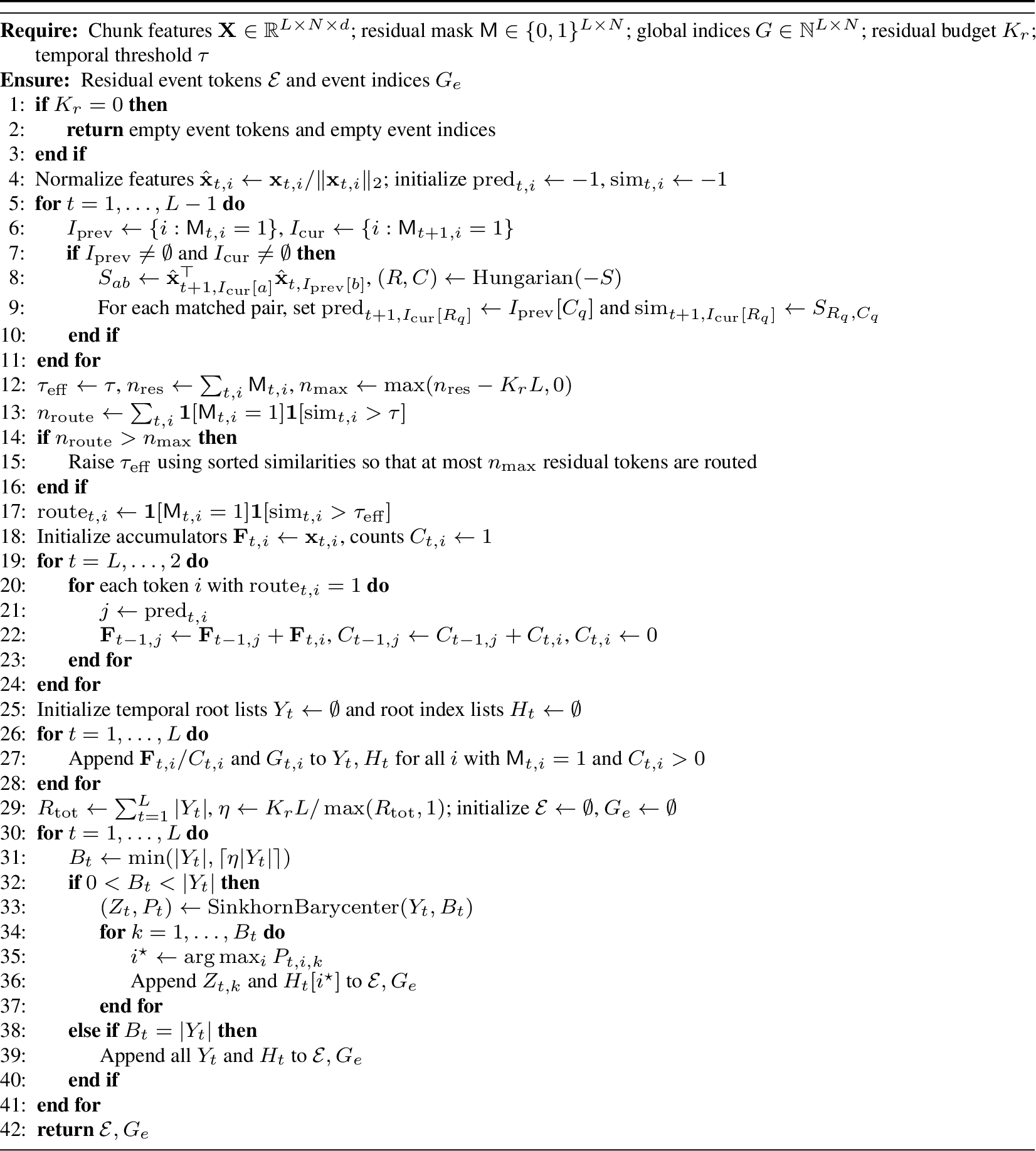
Let \(\operatorname{route}_{t,i}\) indicate whether the residual token \((t,i)\) is routed to a predecessor. Backward accumulation defines each surviving event root as \[\tilde{\mathbf{r}}_q = \frac{1}{|\mathcal{T}_q|} \sum_{\mathbf{r}\in\mathcal{T}_q}\mathbf{r}, \label{eq:app95trajectory95pooling}\tag{20}\] where \(\mathcal{T}_q\) is the residual trajectory ending at root \(q\). TCRC then allocates the residual-event budget across frames proportionally: \[B_t = \min\!\left( M_t,\, \left\lceil \frac{K_rL}{\sum_{u=1}^{L}M_u} M_t \right\rceil \right), \label{eq:app95residual95budget}\tag{21}\] where \(M_t\) is the number of surviving temporal roots in frame \(t\). Frames with \(M_t>B_t\) are further compressed by Sinkhorn barycenter condensation.
5 gives the full residual condensation procedure, including Hungarian matching, adaptive thresholding, backward accumulation, proportional budget allocation, and spatial condensation.
8.3.2 Sinkhorn Barycenter Condensation↩︎
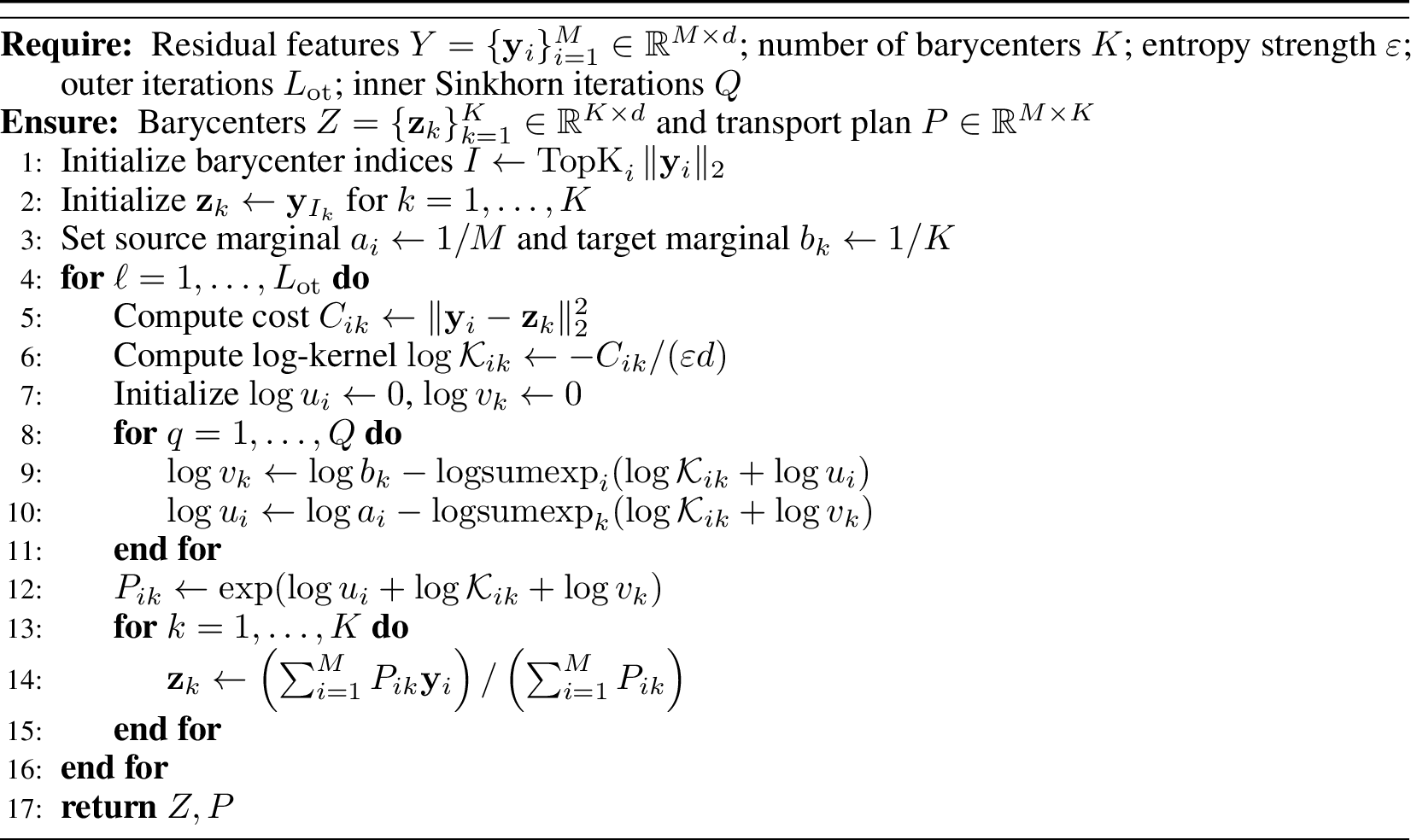
For a frame with \(M\) residual roots \(Y=\{\mathbf{y}_i\}_{i=1}^{M}\) and target budget \(K\), GeoTrace computes \(K\) barycenters \(Z=\{\mathbf{z}_k\}_{k=1}^{K}\) using entropy-regularized optimal transport. With uniform source and target marginals \(a_i=1/M\) and \(b_k=1/K\), the transport plan solves \[P^{\star} = \arg\min_{P\in\mathcal{U}(a,b)} \sum_{i,k}P_{ik}\|\mathbf{y}_i-\mathbf{z}_k\|_2^2 + \varepsilon\sum_{i,k}P_{ik}\log P_{ik}. \label{eq:app95sinkhorn95objective}\tag{22}\] The barycenters are updated by \[\mathbf{z}_k = \frac{\sum_{i=1}^{M}P^{\star}_{ik}\mathbf{y}_i}{\sum_{i=1}^{M}P^{\star}_{ik}}. \label{eq:app95barycenter95update}\tag{23}\] Each barycenter inherits the global index of the source residual root with the largest transport mass: \[g(\mathbf{z}_k) = g\!\left(\mathbf{y}_{\arg\max_i P^{\star}_{ik}}\right). \label{eq:app95barycenter95index}\tag{24}\] 6 provides the solver used in TCRC.
9 Near-Manifold Preservation of TCRC↩︎
This section formalizes the manifold-fidelity intuition behind TCRC. The result is stated as a near-manifold guarantee rather than an exact manifold-membership guarantee, since TCRC only assumes that matched trajectory features and transport-assigned source features lie within local neighborhoods where the visual feature manifold is approximately linear.
9.0.0.1 Notation.
For a closed set \(\mathcal{M}\subset\mathbb{R}^d\), let \[\operatorname{dist}(\mathbf{x},\mathcal{M}) = \inf_{\mathbf{p}\in\mathcal{M}} \|\mathbf{x}-\mathbf{p}\|_2 .\] When the nearest point is unique, we denote it by \(\pi_{\mathcal{M}}(\mathbf{x})\). For a finite set \(A\), let \[\operatorname{diam}(A) = \sup_{\mathbf{x},\mathbf{y}\in A}\|\mathbf{x}-\mathbf{y}\|_2 .\]
Assumption 1 (Local visual feature manifold). The clean residual-token features are supported on a compact \(m\)-dimensional \(C^2\) submanifold \(\mathcal{M}\subset\mathbb{R}^d\). The manifold has reached at least \(\rho_{\mathcal{M}}>0\). The observed raw residual tokens are near \(\mathcal{M}\): for every residual token \(\mathbf{r}\), \[\operatorname{dist}(\mathbf{r},\mathcal{M})\le \eta, \qquad \|\mathbf{r}\|_2\le R .\] We assume \(\eta<\rho_{\mathcal{M}}\), so the nearest-point projection is well-defined in the relevant tubular neighborhood.
Assumption 2 (Temporal locality of accepted trajectories). For every temporal trajectory \(\mathcal{T}_{\ell}\) induced by TCRC, the manifold projections of its raw residual tokens lie in a local chart of radius \(\delta_{\mathrm{temp}}\): \[\operatorname{diam} \left( \left\{ \pi_{\mathcal{M}}(\mathbf{r}):\mathbf{r}\in\mathcal{T}_{\ell} \right\} \right) \le \delta_{\mathrm{temp}}, \qquad \delta_{\mathrm{temp}}\le c\rho_{\mathcal{M}},\] where \(c>0\) is a sufficiently small universal constant.
Assumption 3 (Spatial locality of transport columns). Let \(Y_t=\{\mathbf{y}_{t,i}\}_{i=1}^{M_t}\) be the temporally surviving residual roots in frame \(t\). For the \(k\)-th Sinkhorn barycenter, define normalized column weights \[\lambda_{t,ik} = \frac{P^{\star}_{t,ik}}{\sum_j P^{\star}_{t,jk}}, \qquad \sum_i \lambda_{t,ik}=1 .\] For each column \(k\), there exists a local index set \(I_{t,k}\subseteq\{1,\ldots,M_t\}\) such that \[\sum_{i\in I_{t,k}}\lambda_{t,ik}\ge 1-\gamma_{t,k},\] and the projected local sources satisfy \[\operatorname{diam} \left( \left\{ \pi_{\mathcal{M}}(\mathbf{y}_{t,i}): i\in I_{t,k} \right\} \right) \le \delta_{\mathrm{sp}}, \qquad \delta_{\mathrm{sp}}\le c\rho_{\mathcal{M}} .\] We also assume the temporally surviving roots are bounded and lie in the projection neighborhood: \[\|\mathbf{y}_{t,i}\|_2\le R, \qquad \operatorname{dist}(\mathbf{y}_{t,i},\mathcal{M})<\rho_{\mathcal{M}} .\] When the transport column is entirely local, \(\gamma_{t,k}=0\).
Lemma 1 (Local Euclidean barycenters are near the manifold). Let \(\mathcal{M}\subset\mathbb{R}^d\) be a \(C^2\) submanifold with reach at least \(\rho_{\mathcal{M}}\). There exists a universal constant \(C_0>0\) such that the following holds. Suppose \(\mathbf{x}_1,\ldots,\mathbf{x}_n\in\mathbb{R}^d\) satisfy \[\operatorname{dist}(\mathbf{x}_i,\mathcal{M})\le \xi ,\] and their projections \(\mathbf{p}_i=\pi_{\mathcal{M}}(\mathbf{x}_i)\) lie in a common local chart with \[\operatorname{diam}\{\mathbf{p}_1,\ldots,\mathbf{p}_n\}\le \delta, \qquad \delta\le c\rho_{\mathcal{M}} .\] Then for any convex weights \(\lambda_i\ge 0\), \(\sum_i\lambda_i=1\), the Euclidean barycenter \[\bar{\mathbf{x}} = \sum_{i=1}^{n}\lambda_i\mathbf{x}_i\] satisfies \[\operatorname{dist}(\bar{\mathbf{x}},\mathcal{M}) \le \xi + C_0\frac{\delta^2}{\rho_{\mathcal{M}}}.\]
Proof. Write each point as \[\mathbf{x}_i=\mathbf{p}_i+\mathbf{e}_i, \qquad \mathbf{p}_i=\pi_{\mathcal{M}}(\mathbf{x}_i), \qquad \|\mathbf{e}_i\|_2\le \xi .\] Then \[\bar{\mathbf{x}} = \sum_i\lambda_i\mathbf{p}_i + \sum_i\lambda_i\mathbf{e}_i .\] Since the weights are convex, \[\left\|\sum_i\lambda_i\mathbf{e}_i\right\|_2 \le \sum_i\lambda_i\|\mathbf{e}_i\|_2 \le \xi .\] It remains to bound the distance from \(\sum_i\lambda_i\mathbf{p}_i\) to \(\mathcal{M}\).
Choose a reference point \(\mathbf{p}_0\in\mathcal{M}\) in the local neighborhood and let \(T_{\mathbf{p}_0}\mathcal{M}\) be the tangent space. Since \(\mathcal{M}\) has reached at least \(\rho_{\mathcal{M}}\), for \(\delta\le c\rho_{\mathcal{M}}\), the local patch of \(\mathcal{M}\) around \(\mathbf{p}_0\) can be represented as the graph of a \(C^2\) map \[h:T_{\mathbf{p}_0}\mathcal{M}\rightarrow T_{\mathbf{p}_0}\mathcal{M}^{\perp},\] with \[h(\mathbf{0})=\mathbf{0}, \qquad Dh(\mathbf{0})=\mathbf{0}, \qquad \|D^2 h\|\le \frac{C}{\rho_{\mathcal{M}}},\] for a universal constant \(C>0\). Thus, each projected point can be written as \[\mathbf{p}_i = \mathbf{p}_0+\mathbf{u}_i+h(\mathbf{u}_i),\] where \(\mathbf{u}_i\in T_{\mathbf{p}_0}\mathcal{M}\) and \(\|\mathbf{u}_i-\mathbf{u}_j\|_2=O(\delta)\).
Let \[\bar{\mathbf{u}} = \sum_i\lambda_i\mathbf{u}_i, \qquad \mathbf{q} = \mathbf{p}_0+\bar{\mathbf{u}}+h(\bar{\mathbf{u}})\in\mathcal{M}.\] Then \[\left\| \sum_i\lambda_i\mathbf{p}_i-\mathbf{q} \right\|_2 = \left\| \sum_i\lambda_i h(\mathbf{u}_i)-h(\bar{\mathbf{u}}) \right\|_2 .\] By Taylor’s theorem and the Hessian bound, \[\left\| \sum_i\lambda_i h(\mathbf{u}_i)-h(\bar{\mathbf{u}}) \right\|_2 \le \frac{C}{\rho_{\mathcal{M}}} \sum_i\lambda_i\|\mathbf{u}_i-\bar{\mathbf{u}}\|_2^2 \le C_0\frac{\delta^2}{\rho_{\mathcal{M}}}.\] Therefore, \[\operatorname{dist} \left( \sum_i\lambda_i\mathbf{p}_i,\mathcal{M} \right) \le C_0\frac{\delta^2}{\rho_{\mathcal{M}}}.\] Combining this with the noise bound gives the claim. ◻
Theorem 1 (Near-manifold preservation of TCRC event tokens). Under 1 2 3, every TCRC event token \(\mathbf{z}_{t,k}\) satisfies \[\operatorname{dist}(\mathbf{z}_{t,k},\mathcal{M}) \le \eta + C_0\frac{\delta_{\mathrm{temp}}^2+\delta_{\mathrm{sp}}^2}{\rho_{\mathcal{M}}} + 2R\gamma_{t,k}.\] In particular, when the transport column is entirely local, i.e., \(\gamma_{t,k}=0\), \[\operatorname{dist}(\mathbf{z}_{t,k},\mathcal{M}) \le \eta + C_0\frac{\delta_{\mathrm{temp}}^2+\delta_{\mathrm{sp}}^2}{\rho_{\mathcal{M}}}.\]
Proof. Consider a temporal trajectory \[\mathcal{T}_{\ell} = \{\mathbf{r}_{\ell,1},\ldots,\mathbf{r}_{\ell,n_{\ell}}\}.\] TCRC produces the temporal root \[\tilde{\mathbf{r}}_{\ell} = \frac{1}{n_{\ell}} \sum_{a=1}^{n_{\ell}}\mathbf{r}_{\ell,a}.\] By 1, each raw residual token satisfies \[\operatorname{dist}(\mathbf{r}_{\ell,a},\mathcal{M})\le \eta .\] By 2, the projected trajectory lies in a local chart of diameter at most \(\delta_{\mathrm{temp}}\). Applying 1 with uniform weights gives \[\operatorname{dist}(\tilde{\mathbf{r}}_{\ell},\mathcal{M}) \le \eta + C_0\frac{\delta_{\mathrm{temp}}^2}{\rho_{\mathcal{M}}}.\] Define \[\eta_{\mathrm{temp}} = \eta + C_0\frac{\delta_{\mathrm{temp}}^2}{\rho_{\mathcal{M}}}.\] Thus every temporally surviving residual root \(\mathbf{y}_{t,i}\) is within distance \(\eta_{\mathrm{temp}}\) of \(\mathcal{M}\).
For the \(k\)-th event token in frame \(t\), the Sinkhorn update uses normalized column weights \[\lambda_{t,ik} = \frac{P^{\star}_{t,ik}}{\sum_j P^{\star}_{t,jk}}, \qquad \sum_i\lambda_{t,ik}=1,\] and forms \[\mathbf{z}_{t,k} = \sum_i \lambda_{t,ik}\mathbf{y}_{t,i}.\] Let \(I_{t,k}\) be the local source set from 3, and define its total mass \[\beta_{t,k} = \sum_{i\in I_{t,k}}\lambda_{t,ik}.\] By assumption, \(\beta_{t,k}\ge 1-\gamma_{t,k}\). Define local normalized weights \[\bar{\lambda}_{t,ik} = \frac{\lambda_{t,ik}}{\beta_{t,k}}, \qquad i\in I_{t,k},\] and the purely local barycenter \[\mathbf{z}^{\mathrm{loc}}_{t,k} = \sum_{i\in I_{t,k}}\bar{\lambda}_{t,ik}\mathbf{y}_{t,i}.\] The sources in \(I_{t,k}\) have projected diameter at most \(\delta_{\mathrm{sp}}\), and each \(\mathbf{y}_{t,i}\) is within distance \(\eta_{\mathrm{temp}}\) of \(\mathcal{M}\). Applying 1 again gives \[\operatorname{dist} \left( \mathbf{z}^{\mathrm{loc}}_{t,k},\mathcal{M} \right) \le \eta_{\mathrm{temp}} + C_0\frac{\delta_{\mathrm{sp}}^2}{\rho_{\mathcal{M}}}.\]
Entropy-regularized transport can assign small positive mass to nonlocal sources, so we account for the tail explicitly. If \(\beta_{t,k}<1\), let \[\mathbf{z}^{\mathrm{tail}}_{t,k} = \frac{1}{1-\beta_{t,k}} \sum_{i\notin I_{t,k}}\lambda_{t,ik}\mathbf{y}_{t,i};\] Otherwise, this term is unused. Then \[\mathbf{z}_{t,k} = \beta_{t,k}\mathbf{z}^{\mathrm{loc}}_{t,k} + (1-\beta_{t,k})\mathbf{z}^{\mathrm{tail}}_{t,k}.\] Since both \(\mathbf{z}^{\mathrm{loc}}_{t,k}\) and \(\mathbf{z}^{\mathrm{tail}}_{t,k}\) are convex combinations of vectors with norm at most \(R\), \[\|\mathbf{z}^{\mathrm{loc}}_{t,k}\|_2\le R, \qquad \|\mathbf{z}^{\mathrm{tail}}_{t,k}\|_2\le R.\] Therefore, \[\|\mathbf{z}_{t,k}-\mathbf{z}^{\mathrm{loc}}_{t,k}\|_2 = (1-\beta_{t,k}) \| \mathbf{z}^{\mathrm{tail}}_{t,k} - \mathbf{z}^{\mathrm{loc}}_{t,k} \|_2 \le 2R(1-\beta_{t,k}) \le 2R\gamma_{t,k}.\] Using the triangle inequality, \[\operatorname{dist}(\mathbf{z}_{t,k},\mathcal{M}) \le \operatorname{dist} \left( \mathbf{z}^{\mathrm{loc}}_{t,k},\mathcal{M} \right) + \|\mathbf{z}_{t,k}-\mathbf{z}^{\mathrm{loc}}_{t,k}\|_2 .\] Substituting the previous bounds yields the theorem. ◻
Corollary 1 (Temporal threshold controls trajectory diameter). Assume residual features are \(\ell_2\)-normalized before temporal matching. If an accepted temporal edge satisfies \[\cos(\mathbf{r}_{t+1,i},\mathbf{r}_{t,j})\ge \tau_{\mathrm{eff}},\] then \[\|\mathbf{r}_{t+1,i}-\mathbf{r}_{t,j}\|_2 \le \sqrt{2(1-\tau_{\mathrm{eff}})} .\] Consequently, if an accepted trajectory has at most \(H\) temporal edges, then its raw Euclidean diameter is bounded by \[\operatorname{diam}(\mathcal{T}_{\ell}) \le H\sqrt{2(1-\tau_{\mathrm{eff}})} .\] Up to the near-manifold noise radius, the projected trajectory diameter \(\delta_{\mathrm{temp}}\) is therefore controlled by the temporal threshold and the maximum trajectory length.
Proof. For normalized vectors \(\mathbf{a}\) and \(\mathbf{b}\), \[\|\mathbf{a}-\mathbf{b}\|_2^2 = \|\mathbf{a}\|_2^2+\|\mathbf{b}\|_2^2-2\langle \mathbf{a},\mathbf{b}\rangle = 2(1-\cos(\mathbf{a},\mathbf{b})).\] Thus an accepted edge with cosine similarity at least \(\tau_{\mathrm{eff}}\) has Euclidean length at most \(\sqrt{2(1-\tau_{\mathrm{eff}})}\). The trajectory-diameter bound follows from the triangle inequality along a path with at most \(H\) edges. ◻
Corollary 2 (Why TCRC is more manifold-faithful than unconstrained fusion). Consider an unconstrained residual fusion rule that averages a group of residual tokens whose projected diameter is \(\Delta\). Under the same manifold assumptions, 1 gives the generic drift bound \[\operatorname{dist}(\bar{\mathbf{r}},\mathcal{M}) \le \eta + C_0\frac{\Delta^2}{\rho_{\mathcal{M}}}.\] TCRC replaces the unconstrained group diameter \(\Delta\) by the controlled temporal and spatial radii \(\delta_{\mathrm{temp}}\) and \(\delta_{\mathrm{sp}}\). Therefore, when \[\delta_{\mathrm{temp}}^2+\delta_{\mathrm{sp}}^2 \ll \Delta^2,\] TCRC has a strictly smaller near-manifold drift bound.
Proof. The unconstrained bound follows directly from 1 by setting the group diameter to \(\Delta\). The TCRC bound follows from 1. Thresholded one-to-one temporal routing prevents tree-like many-to-one collapse across frames, so each temporal event is a path of high-confidence local correspondences rather than an arbitrary mixture of residual tokens. The Sinkhorn step further penalizes long transport through the squared Euclidean cost, and 3 captures the resulting local transport-column concentration. Comparing the two bounds gives the claim. ◻
9.0.0.2 Traceability of inherited indices.
The dominant-source index assignment \[g(\mathbf{z}_{t,k}) = g\!\left( \mathbf{y}_{t,\arg\max_i P^{\star}_{t,ik}} \right)\] does not by itself imply manifold membership. Its role is provenance: every spatially condensed event token is associated with the source residual root that contributes the largest transport mass. Together with one-to-one temporal routing, this provides a traceable chain from each event token back to observed residual evidence.
9.0.0.3 Limitations.
The result is local. It does not prove that Euclidean averages lie exactly on \(\mathcal{M}\), nor does it guarantee a small drift when residual groups span distant semantic modes. The essential assumptions are: raw residual features are near a regular feature manifold, accepted temporal trajectories remain local, and each transport column has most of its mass on a local residual group. Entropic transport assigns positive mass broadly in principle, so 1 explicitly includes the tail term \(2R\gamma_{t,k}\). If \(\gamma_{t,k}\), \(\delta_{\mathrm{temp}}\), or \(\delta_{\mathrm{sp}}\) becomes large, the bound correspondingly weakens. This is why TCRC uses thresholded one-to-one matching and transport-based condensation rather than unconstrained residual fusion.
10 Token Budget Alignment↩︎
GeoTrace adopts an expansion-then-pruning protocol for fair token-budget alignment. It first retains a mildly expanded visual sequence before LLM prefill, and then applies inner-LLM pruning from layer \(\ell_p\) onward so that the average number of visual tokens processed by each Transformer layer matches the target budget. We use this average layer-wise token count as a proxy for comparable computational cost between prefill-stage compression and inner-LLM acceleration methods.
For the Video LLMs evaluated in this paper, the Transformer FLOPs can be approximated as \[\mathrm{FLOPs} = L \times \left( 2nd^2(1+g/h) +2n^2d +3ndm \right), \label{eq:app95transformer95flops}\tag{25}\] where \(L\) is the number of Transformer layers, \(n\) is the sequence length, \(d\) is the hidden dimension, \(m\) is the FFN intermediate dimension, \(g\) is the number of key/value heads, and \(h\) is the number of attention heads. Since visual tokens dominate the sequence length in our video setting, \(n\) is approximated by the number of visual tokens.
Let \(\bar N_{\mathrm{avg}}\) denote the target average number of visual tokens per Transformer layer, \(M\) the number of visual tokens entering LLM prefill after GeoTrace compression, \(\ell_p\) the first layer where inner-LLM pruning is applied, and \(N_{\mathrm{ret}}\) the number of visual tokens retained after pruning. The total layer-wise visual-token count satisfies \[\bar N_{\mathrm{avg}} L = M\ell_p + N_{\mathrm{ret}}(L-\ell_p). \label{eq:app95budget95alignment}\tag{26}\]
Under the expansion stage, the prefill-stage token count is parameterized as \[M=f_e\bar N_{\mathrm{avg}}, \label{eq:app95expansion95factor}\tag{27}\] where \(f_e\) is the expansion factor. Substituting 27 into 26 gives the number of visual tokens retained after inner-LLM pruning: \[N_{\mathrm{ret}} = \frac{\bar N_{\mathrm{avg}}(L-f_e\ell_p)}{L-\ell_p}. \label{eq:app95inner95retained95tokens}\tag{28}\]
The corresponding inner-LLM visual-token retention ratio is \[\rho_{\mathrm{LLM}} = \frac{N_{\mathrm{ret}}}{M} = \frac{L-f_e\ell_p}{f_e(L-\ell_p)}. \label{eq:app95inner95pruning95ratio}\tag{29}\]
This alignment allows GeoTrace to preserve a richer visual sequence before LLM prefilling, while subsequent layer-wise pruning restores the same average layer-wise visual-token budget used by competing acceleration methods.
In all main experiments, we instantiate this protocol with expansion factor \(f_e=1.25\), inner-LLM pruning layer \(\ell_p=20\), and inner-LLM visual-token retention ratio \(\rho_{\mathrm{LLM}}=0.3\). In other words, GeoTrace first keeps a mildly expanded visual sequence before the LLM, begins layer-wise visual-token pruning at the 20th Transformer layer, and keeps \(30\%\) of the expanded visual tokens after this pruning step. These three hyperparameters control only the budget-alignment protocol: they determine how the expanded GeoTrace output is reconciled with the target average layer-wise token budget, while CFPA and TCRC determine which visual evidence is preserved or condensed before LLM inference.
11 Complexity↩︎
Let \(L\) be the number of frames in a chunk, \(N\) the number of visual tokens per frame, \(d\) the feature dimension, \(B\) the CFPA beam size, and \(K_s\) the skeleton budget. CFPA computes pairwise cosine similarities within each frame and then runs beam expansion, giving the dominant cost \[O(LN^2d + LBK_sN). \label{eq:app95cfpa95complexity}\tag{30}\] TCRC computes adjacent-frame residual similarities and performs one-to-one matching. If \(R_t\) is the number of residual tokens in frame \(t\), the similarity computation costs \[O\!\left(\sum_{t=1}^{L-1}R_tR_{t+1}d\right), \label{eq:app95similarity95complexity}\tag{31}\] and Hungarian matching adds a cubic term in the smaller residual-set size for each adjacent frame. Sinkhorn barycenter condensation is applied only to frames whose temporal residual roots exceed their allocated budgets. For a frame with \(M_t\) temporal roots, target budget \(B_t\), \(L_{\mathrm{ot}}\) outer iterations, and \(Q\) Sinkhorn iterations, the dominant cost is \[O(L_{\mathrm{ot}}Q M_tB_t + L_{\mathrm{ot}}M_tB_td). \label{eq:app95sinkhorn95complexity}\tag{32}\] All operations are performed once before LLM prefill. The compressed visual sequence then reduces subsequent attention computation and KV-cache usage in the language model.
12 Qualitative Demonstrations↩︎
This section provides qualitative demonstrations of the two GeoTrace components. The visualizations are intended to make the behavior of CFPA and TCRC easier to inspect beyond aggregate benchmark numbers. CFPA is expected to preserve a compact set of exact skeleton tokens that jointly cover salient, context-consistent, and complementary evidence. TCRC is expected to compress the non-skeleton residual evidence through locally coherent temporal routes, so that the resulting event tokens remain traceable to concrete source regions rather than becoming unconstrained mixtures.
12.0.0.1 CFPA skeleton tokens.
7 visualizes CFPA selections on three video instances. Each row corresponds to one video, showing its original frames and the corresponding CFPA-selected skeleton tokens. The selected skeleton tokens cover salient foreground evidence such as faces, hands, and task-relevant objects, while also retaining complementary context tokens from the surrounding scene. This behavior is consistent with the CFPA objective: skeleton tokens are not selected only by saliency alone, but by the combination of saliency, contextual consistency, and feature-space coverage. Compared with a purely attention-based selector, this qualitative behavior is important because the visual budget should not collapse onto a small number of locally dominant regions. The preserved tokens instead form a sparse but spatially distributed scaffold for the video chunk, giving the downstream LLM access to exact visual features that summarize both the central object evidence and the surrounding layout needed for reasoning.
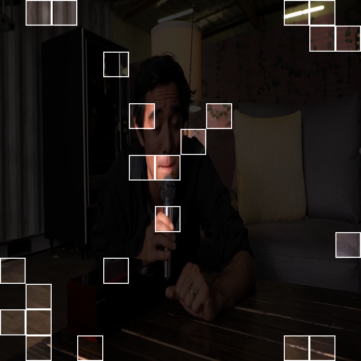
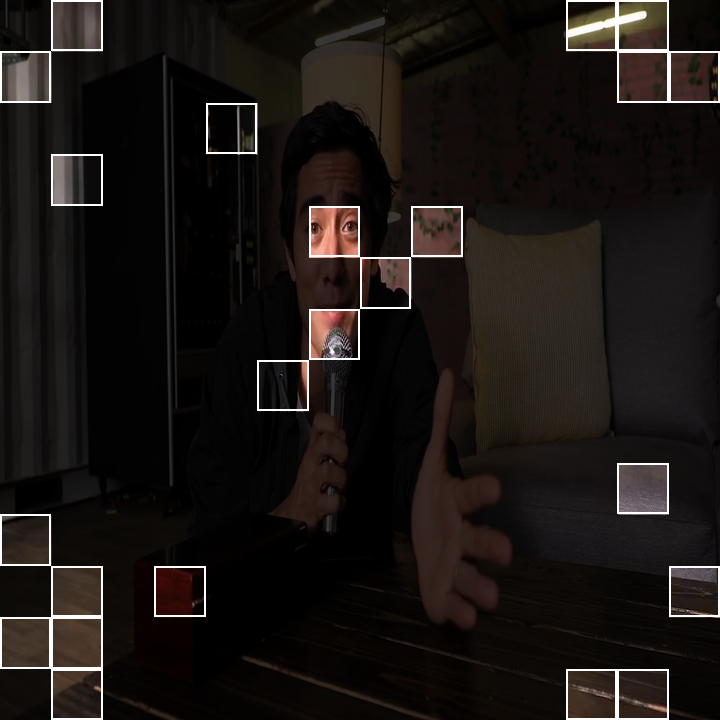
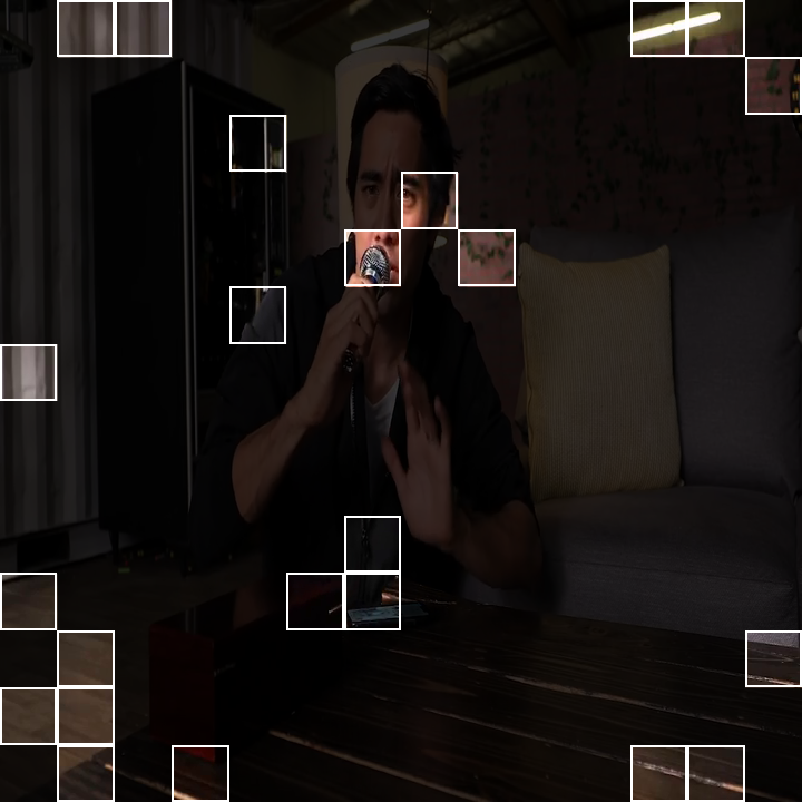
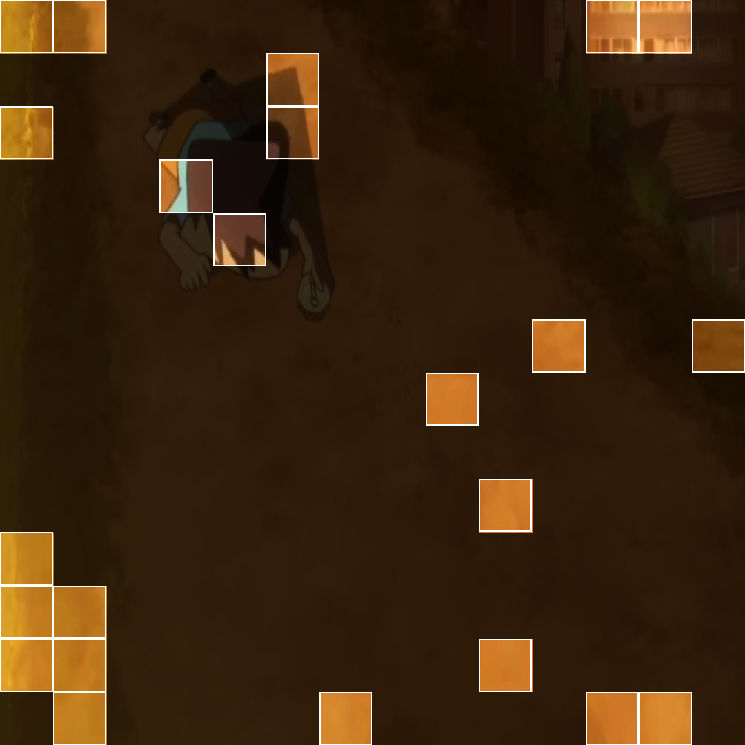





Figure 7: Qualitative CFPA demonstrations. Each row shows one video instance, with white boxes indicating selected skeleton tokens in three frames. CFPA preserves exact visual tokens that jointly cover salient entities and complementary scene context, rather than collapsing the budget onto only the most salient local region..
12.0.0.2 TCRC temporal routes.
8 shows successful TCRC routing examples. Colored boxes and lines indicate residual-token trajectories accepted by one-to-one temporal matching. In these cases, the routed tokens follow visually coherent evidence across adjacent frames, so temporal pooling condenses repeated residual information while preserving a traceable path back to observed video tokens. These examples illustrate the intended role of TCRC as a residual-event compressor rather than a generic token merger. By enforcing one-to-one matching before temporal pooling, TCRC avoids many-to-one collapse, where several visually distinct residual regions from the current frame are absorbed into the same predecessor. The accepted routes, therefore, behave like short local trajectories: they remove repeated evidence across nearby frames while keeping a clear provenance chain for each condensed event token.
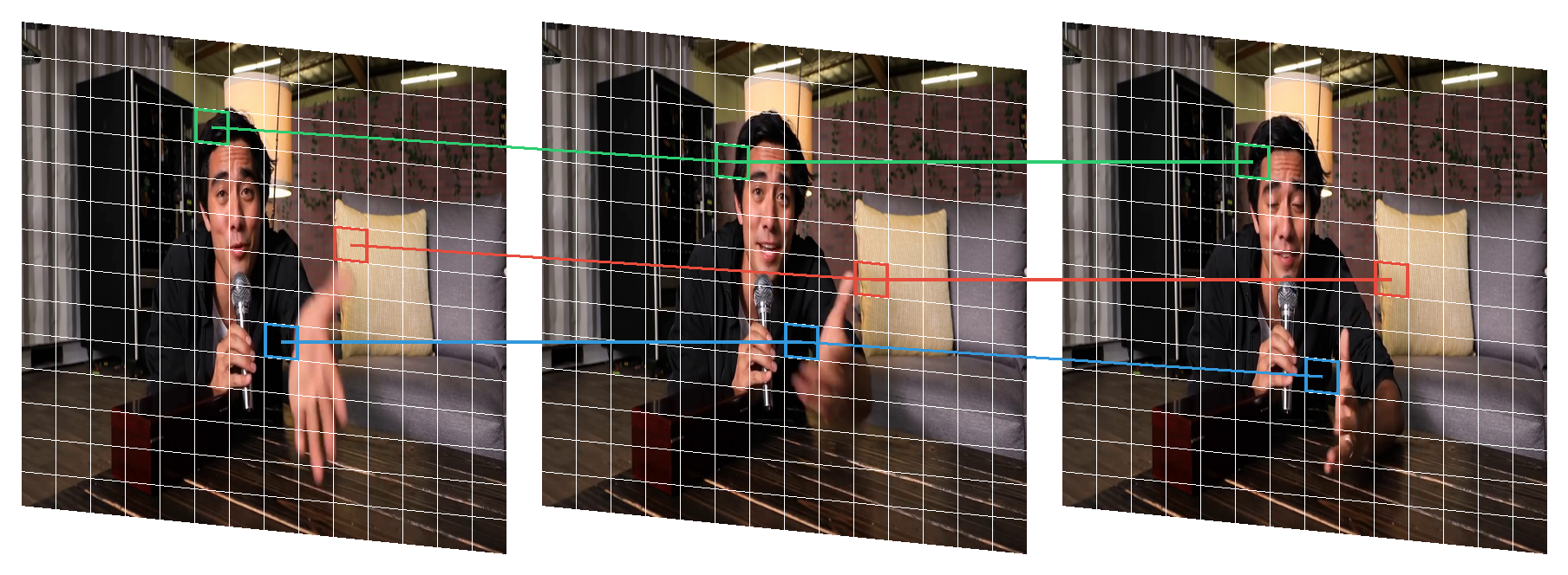
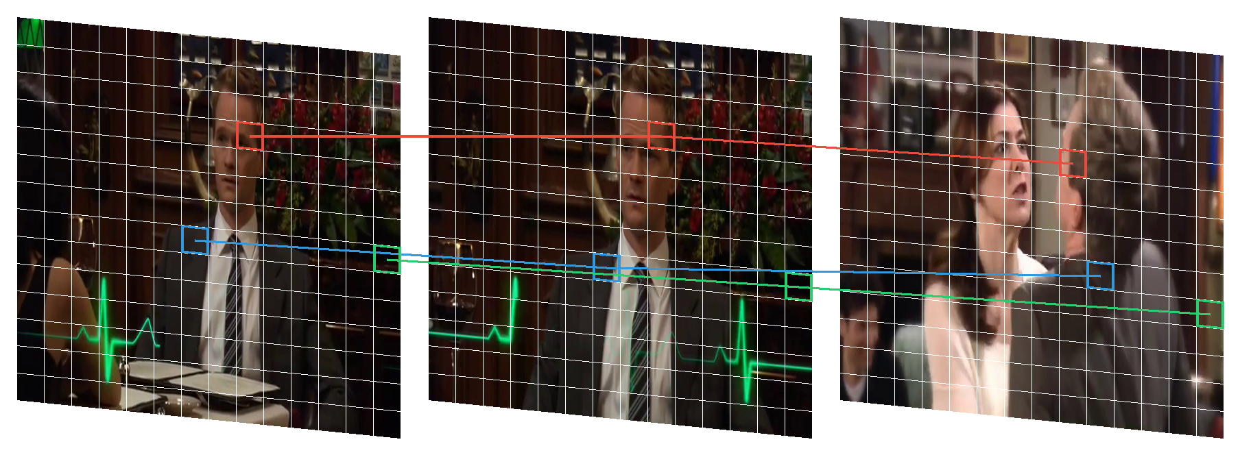
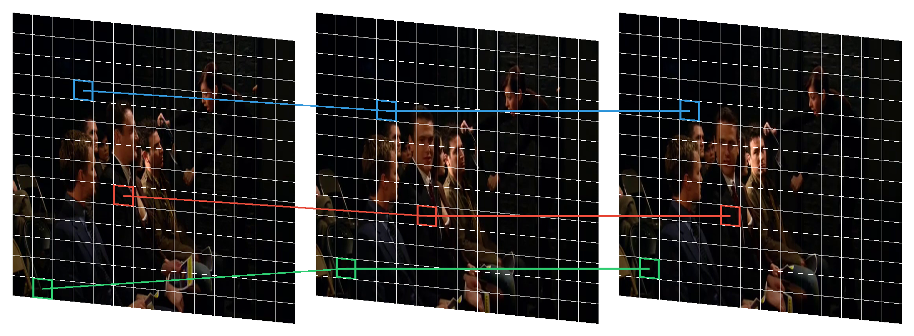
Figure 8: Successful TCRC trajectory demonstrations. Accepted residual-token routes connect high-confidence, one-to-one temporal correspondences across frames. The examples illustrate how TCRC compresses repeated residual evidence while keeping event tokens traceable to concrete source regions..
9 shows two challenging cases. These examples contain larger viewpoint changes, ambiguous local appearance, or semantic transitions that can make residual matching less reliable. Such cases motivate the use of an effective temporal threshold and one-to-one matching: weak or ambiguous correspondences should be filtered or fragmented rather than merged aggressively into a single residual event token. They also clarify why TCRC is paired with CFPA. Even when residual trajectories are incomplete, the exact skeleton tokens preserved by CFPA still provide stable visual anchors, while TCRC only condenses the residual evidence that satisfies the matching criterion. This design makes the failure mode more localized: uncertain residual evidence may lead to incomplete or fragmented event tokens, but it is less likely to overwrite the exact skeleton anchors preserved by CFPA or dominate the final visual representation.
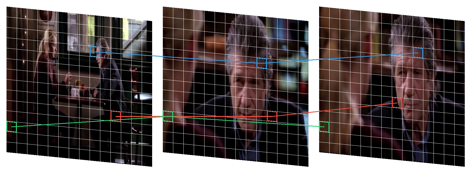
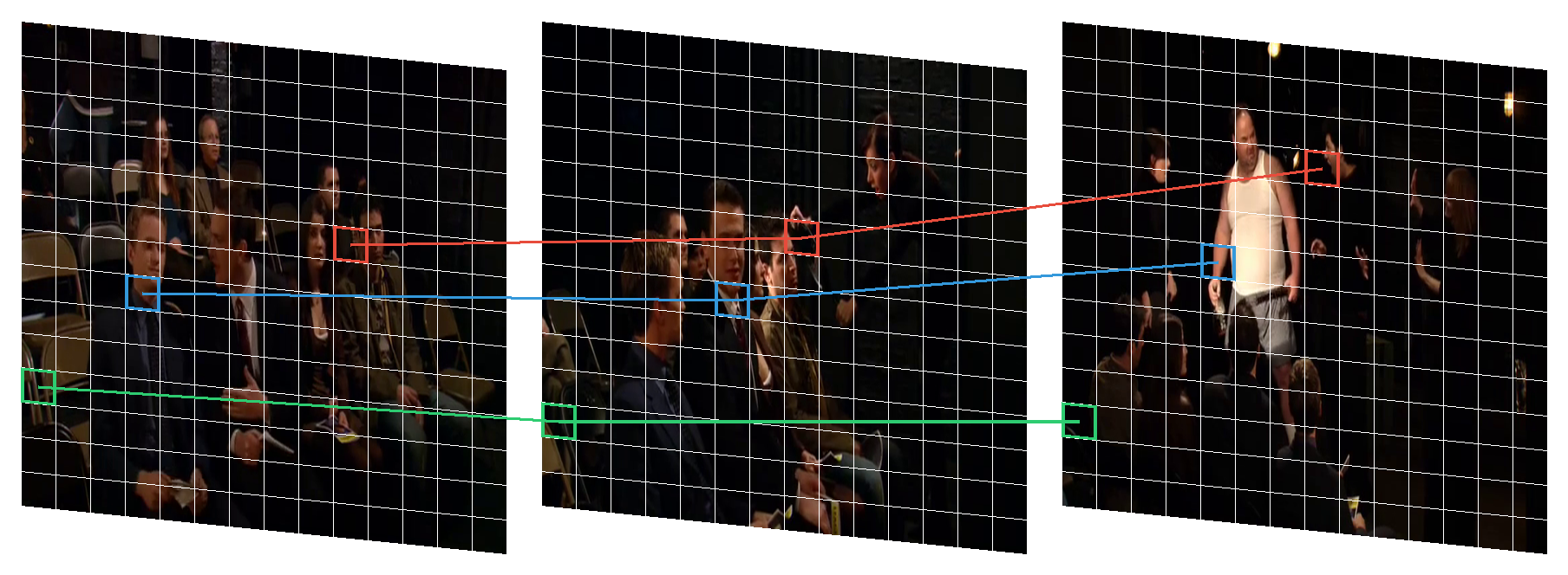
Figure 9: Challenging TCRC routing cases. Large appearance changes or ambiguous regions can make residual trajectories less reliable. These cases illustrate why TCRC uses thresholded one-to-one routing instead of unconstrained many-to-one fusion..
13 Limitations↩︎
GeoTrace is evaluated on four representative Video LLMs and four widely used video understanding benchmarks, covering both fixed-grid and dynamic-resolution visual processing settings. Due to computational constraints, we have not yet evaluated GeoTrace on substantially larger Video LLMs, larger-scale benchmark suites, or extremely long-context video settings. Extending the evaluation to larger models and more diverse deployment scenarios would further clarify how the proposed skeleton preservation and residual condensation mechanisms scale.
GeoTrace is designed as a training-free framework and therefore relies on the visual features provided by the frozen vision encoder. This design makes the method easy to deploy across different Video LLMs without additional training, but its behavior may still depend on the geometry and domain coverage of the underlying visual feature space. Future work may study feature-space diagnostics for token compression, such as estimating when saliency, context consistency, or trajectory matching is reliable, and using these signals to adapt the balance between skeleton preservation and residual condensation.
In the current implementation, GeoTrace uses fixed token allocation, temporal thresholding, and budget-alignment settings across videos. These fixed settings are chosen for simplicity and fair comparison, and they work well across the evaluated benchmarks. Nevertheless, videos can vary substantially in motion density, scene complexity, and temporal structure. Adaptive token budgeting or video-dependent compression policies may further improve the accuracy-efficiency trade-off.
Finally, our experiments focus on offline video understanding. Applying GeoTrace to streaming video inference, online token updating, and memory-constrained real-time deployment remains an interesting direction. These settings may require incremental trajectory construction and dynamic budget adjustment, which we leave for future work.