STEAM: Stable Self-Training with Elastic Matching and Adaptive Purification
July 10, 2026
Abstract
Cross-view geo-localization (CVGL) aims to achieve GPS-free localization by matching drone-view images with corresponding satellite-view images. Existing supervised methods rely on large-scale manually annotated cross-view image pairs, making them costly and difficult to scale. In contrast, existing unsupervised approaches typically depend on generative models or clustering-based stage-wise optimization, which are prone to distribution bias and the accumulation of noisy pseudo-labels. To address these limitations, we propose STEAM (Stable Self-Training with Elastic Matching and Adaptive Purification), an end-to-end unsupervised cross-view geo-localization framework that performs self-training directly on real drone and satellite images. Specifically, the proposed Stable Spatial-Aware Module enhances the stability of feature representations, Elastic Matching discovers high-quality cross-view pseudo-labels, and Adaptive Purification dynamically maintains a reliable pseudo-label repository throughout the self-training process. Extensive experiments on the University-1652 and SUES-200 benchmarks demonstrate that STEAM achieves state-of-the-art performance among all existing unsupervised methods and delivers performance comparable to supervised approaches, validating the effectiveness and superiority of the proposed framework. The source code is available at https://github.com/wsx-heu/STEAM.git.
1 Introduction↩︎
Cross-view geo-localization (CVGL) aims to achieve GPS-free localization by matching a query image (e.g., a drone-view image) with its corresponding gallery image (e.g., a satellite-view image) in a large-scale image database [1]. As a visual localization technique, CVGL has attracted increasing attention due to its broad applications in autonomous drone navigation, autonomous driving, disaster response, military reconnaissance, and smart cities [2]. However, the substantial viewpoint discrepancy, resolution inconsistency, and appearance variation between drone and satellite images make this task highly challenging [3], [4].
Recent advances in deep learning have significantly promoted the development of cross-view geo-localization. Numerous supervised methods have been proposed, which learn discriminative cross-view feature representations from manually annotated drone–satellite image pairs to achieve accurate localization [5], [6]. However, constructing large-scale paired datasets requires expensive sensing equipment and labor-intensive manual annotation, resulting in high data collection costs [7], [8]. Consequently, learning effective cross-view feature representations without relying on manually paired data has become an important research direction in cross-view geo-localization.
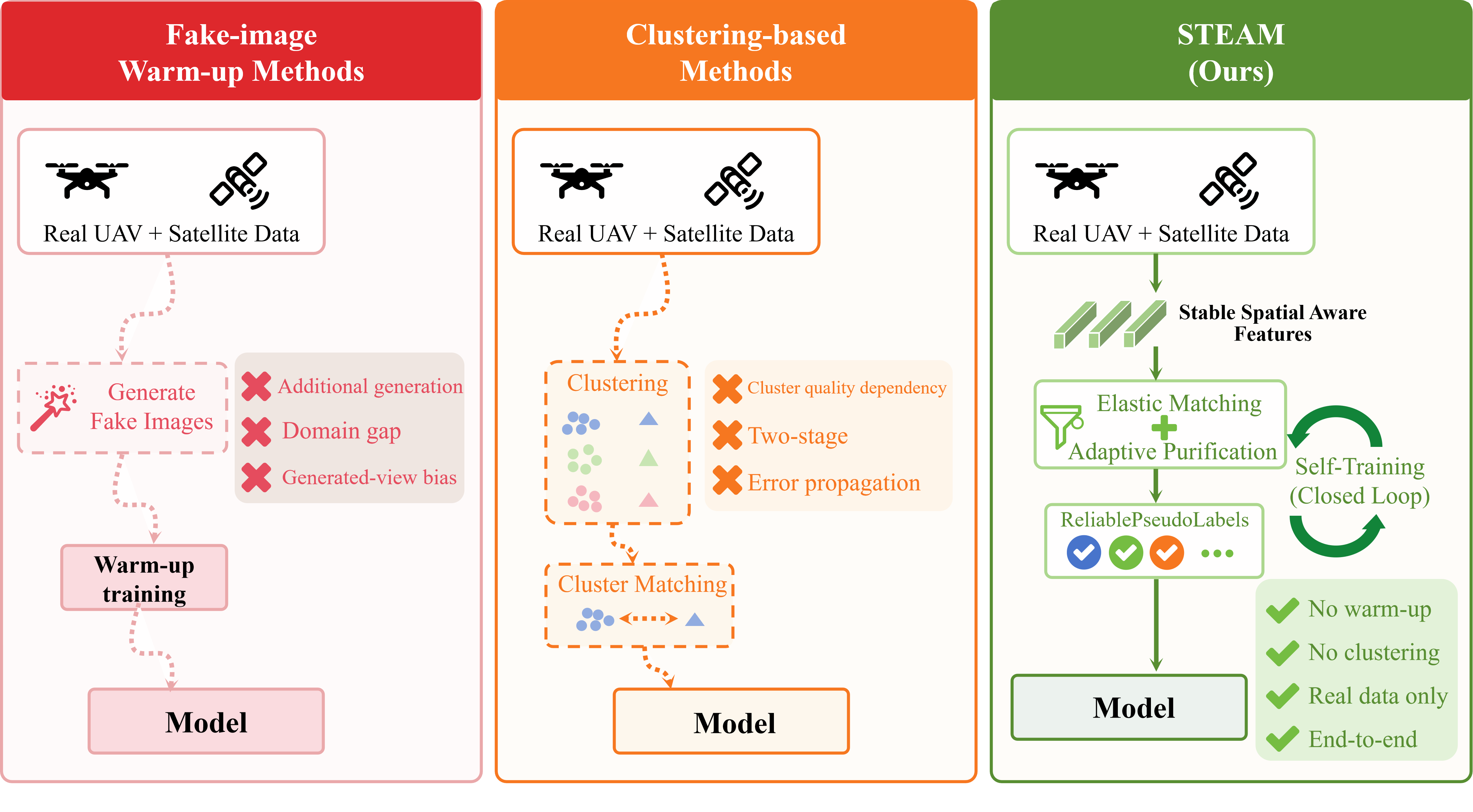
To eliminate the dependency on manual annotations, several unsupervised cross-view geo-localization (UCVGL) methods have recently been proposed, including fake-image warm-up methods [7] and clustering-based methods [9], [10]. Although these methods substantially alleviate the reliance on labeled data and achieve promising performance, they still suffer from notable limitations. As illustrated in Fig. 1, fake-image warm-up methods generally require additional image generation modules, resulting in domain gaps and the distribution bias introduced by generated views. In contrast, clustering-driven two-stage methods are sensitive to hyperparameter selection and depend on clustering quality. More importantly, noisy clusters generated during the early training stage tend to propagate and accumulate throughout subsequent cross-view representation learning, ultimately degrading localization performance.
To address these limitations, we propose an end-to-end UCVGL framework, termed STEAM (Stable Self-Training with Elastic Matching and Adaptive Purification). Unlike previous methods, STEAM performs self-training directly on real drone and satellite images without requiring fake-image generation, clustering initialization, or complicated stage-wise optimization. These three components work in concert: the Stable Spatial-Aware Module provides robust feature representations, Elastic Matching discovers high-quality cross-view pseudo-labels, and Adaptive Purification maintains a reliable repository of cross-view correspondences throughout self-training. The main contributions of this paper are summarized as follows:
We propose the Stable Spatial-Aware Module, which enhances the stability of feature representations via nonlinear multi-head spatial attention, providing robust representations for long-term self-training.
We propose an Elastic Matching mechanism that combines Bidirectional Top-\(K\) Soft Matching with Dynamic Threshold Filtering to discover high-quality cross-view pseudo-labels, improving pseudo-label coverage while maintaining label correctness.
We propose an Adaptive Purification mechanism that dynamically maintains a reliable pseudo-label repository through Confidence-aware Update, Age-aware Update, and Expired Label Removal, effectively suppressing the accumulation of erroneous supervision during self-training.
2 Related Work↩︎
2.1 Supervised Cross-View Geo-Localization↩︎
Supervised cross-view geo-localization has achieved remarkable progress by learning discriminative representations from manually annotated drone–satellite image pairs [11]–[14]. The release of the University-1652 [15] benchmark established the first large-scale evaluation platform and significantly accelerated the development of this field.
Early studies focused on reducing geometric discrepancies using deep neural networks [16]–[19]. Subsequent works attempted explicit viewpoint transformation and view synthesis [20]–[22], such as PCL [23] with perspective transformation, and later FSRA [24] with Vision Transformer for region-level alignment. More recent methods have shifted toward feature representation learning and optimization strategies, including multi-scale contextual modeling [25], symmetric contrastive learning with hard negative sampling [3], domain alignment and scene consistency [26], query-driven fine-tuning [27], and foundation model adaptation [28].
Despite their impressive accuracy [29], supervised methods rely heavily on manually annotated pairs, incurring substantial data collection costs [9], [30] and motivating increasing interest in UCVGL [15], [31], [32].
2.2 Unsupervised Cross-View Geo-Localization↩︎
To alleviate the dependence on manual annotations, numerous unsupervised methods have been proposed for cross-view geo-localization [33]–[36]. Existing approaches can be broadly categorized into two main streams.
Fake-image warm-up methods reduce viewpoint discrepancies through image synthesis [23], [37], [38]. For instance, Li et al. [7] construct pseudo pairs by transforming ground panoramas into bird’s-eye views and generating satellite-style images via CycleGAN. Clustering-based methods generate intra-view pseudo-labels and establish cross-view correspondences through association strategies [39], [40]. Representative frameworks include C2F [9], which progressively aligns features via intra-view clustering and inter-view matching, and UniABG [10], which introduces adversarial learning and heterogeneous graph filtering to enhance association reliability. More recently, training-free reconstruction approaches [8], [41] have emerged, such as a 3D Gaussian Splatting framework [8] that reconstructs scenes from drone images and renders satellite views for zero-shot matching.
Overall, although existing UCVGL methods have achieved remarkable progress, substantial differences still exist among various technical paradigms in terms of feature learning and cross-view association mechanisms. Developing a stable and efficient self-training framework without relying on additional generative models, clustering initialization, or complicated stage-wise optimization remains an important research direction for UCVGL.
3 Method↩︎
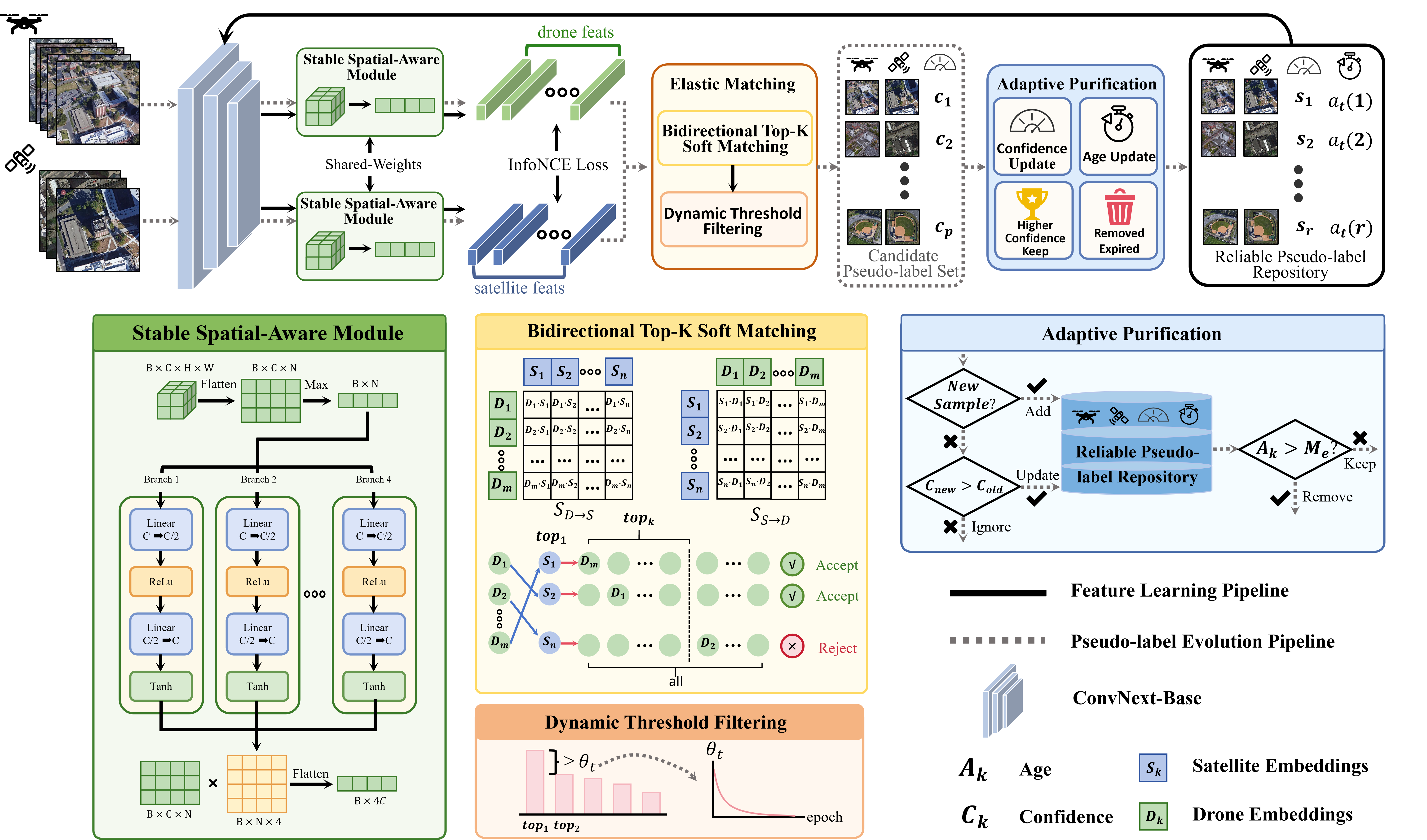
We propose STEAM (Stable Self-Training with Elastic Matching and Adaptive Purification), a self-training framework for UCVGL. STEAM performs end-to-end learning directly on unpaired drone and satellite images and progressively aligns the cross-view feature space through iterative pseudo-label generation and refinement. In the following, we first present the problem formulation and the overall pipeline, and then describe each component in detail.
Problem Formulation. Let \(X_d=\{x_i^d\}_{i=1}^{N_d}\) and \(X_s=\{x_j^s\}_{j=1}^{N_s}\) denote the sets of unlabeled drone images and unlabeled satellite images, respectively, where \(N_d\) and \(N_s\) represent the numbers of samples in each domain. No cross-view correspondence annotations are provided during training. Since multiple drone images captured from different viewpoints and flight heights may correspond to the same satellite image, UCVGL is naturally formulated as a many-to-one cross-view matching problem.
3.1 Overview of STEAM↩︎
As illustrated in Fig. 2, STEAM consists of three components: the Stable Spatial-Aware Module (SSA), Elastic Matching (ElMa), and Adaptive Purification (AdPu). By iteratively refining pseudo-labels and feature representations, STEAM progressively aligns the cross-view feature space in a closed-loop self-training manner. At iteration \(t\), the SSA first extracts feature representations from the drone and satellite images: \[(Z_t^d,Z_t^s)=f_{\mathrm{SSA}}(X^d,X^s),\] based on the current feature space, the Elastic Matching module generates a candidate pseudo-label set: \[P_t=f_{\mathrm{ElMa}}(Z_t^d,Z_t^s),\] where \(P_t\) denotes the candidate pseudo-label set. To improve pseudo-label stability, Adaptive Purification dynamically maintains the candidate pseudo-labels by incorporating historical information, yielding a reliable pseudo-label repository: \[R_t=f_{\mathrm{AdPu}}(P_t,R_{t-1}),\] where \(R_t\) denotes the reliable pseudo-label repository. Using the training pairs constructed from \(R_t\) and the InfoNCE loss, the model is then optimized.
3.2 Stable Spatial-Aware Module↩︎
To ensure feature stability under iteratively updated pseudo-labels, we propose SSA based on the simplified SAFA architecture [7]. By introducing nonlinear constraints on attention responses, SSA suppresses extreme or abnormal attention responses caused by noisy pseudo-labels, thereby enhancing feature stability.
Given an input image \(x\in\mathbb{R}^{H\times W\times3}\), a ConvNeXt-Base backbone is first employed to extract dense feature maps: \[x_{b}=f_{\mathrm{backbone}}(x)\in\mathbb{R}^{C\times H'\times W'},\] where \(C\) denotes the number of channels, and \(H'\) and \(W'\) are the spatial dimensions of the feature map. The feature map is then flattened along the spatial dimension to obtain \(x_{f}=f_{\mathrm{Flatten}}(x_{b})\in\mathbb{R}^{C\times N}\), where \(N=H'\times W'\) denotes the number of spatial locations. To obtain a global image descriptor, max pooling is first applied to aggregate spatial features: \[x_p=f_{\mathrm{pooling}}(x_{f})\in\mathbb{R}^{C}.\]
\(M\) independent attention heads are employed to generate spatial attention weights, \(m=1,\ldots,M,\) \[a_m=\tanh\left(W_2^m\cdot\mathrm{ReLU}\left(W_1^m x_p\right)\right)\in\mathbb{R}^{N},\] where \(W_1^m\) and \(W_2^m\) are learnable parameters. The outputs of all attention heads are concatenated to form the spatial attention matrix: \(A=[a_1,a_2,\ldots,a_M]\in\mathbb{R}^{N\times M}\). The attention matrix is then used to aggregate spatial features: \[x_h=x_{f}\times A\in\mathbb{R}^{C\times M}.\]
The resulting feature matrix is flattened to obtain the final global representation: \(z=f_{\mathrm{Flatten}}(x_h)\in\mathbb{R}^{C\times M}\). Accordingly, the drone and satellite branches produce feature sets: \(Z_d=\{z_i^d\},\quad Z_s=\{z_i^s\}\). SSA establishes a stable feature space for subsequent pseudo-label generation, providing reliable representations for cross-view self-training. The drone and satellite branches share the same SSA parameters to enforce cross-view feature consistency.
3.3 Elastic Matching↩︎
Due to the inherent many-to-one correspondence in cross-view geo-localization, conventional mutual nearest-neighbor matching tends to miss a large number of potential positive pairs, while relying solely on nearest neighbors may introduce noisy supervision. To address this issue, we propose an Elastic Matching (ElMa) strategy, which discovers high-quality pseudo-labels through Bidirectional Top-\(K\) Soft Matching and Dynamic Threshold Filtering.
Bidirectional Top-\(K\) Soft Matching. Before each training round, the current model is used to extract feature representations of all drone and satellite images, denoted by \(Z_d\) and \(Z_s\), respectively. The similarity matrices from drone to satellite and satellite to drone are computed as \(S_{d\rightarrow s} = Z_d Z_s^\top,\quad S_{s\rightarrow d} = Z_s Z_d^\top\). For a drone image \(i\), its nearest satellite image is determined by \(j_1 = \arg\max_j S_{d\rightarrow s}(i,j)\). Since a satellite image may correspond to multiple drone images captured from different viewpoints or altitudes, enforcing strict mutual nearest-neighbor matching would discard many valid correspondences. Therefore, instead of requiring a mutual nearest-neighbor relationship, we only require that drone image \(i\) appears in the Top-\(K\) most similar drone images of satellite image \(j_1\):
\[\mathrm{Match}(i) = \mathbb{I}\big[i \in \mathrm{TopK}(S_{s\rightarrow d}(j_1,:))\big],\] where \(K\) denotes the number of nearest neighbors. The influence of \(K\) is further analyzed in Fig 4.
Dynamic Threshold Filtering. Although Bidirectional Top-\(K\) Soft Matching improves pseudo-label coverage, incorrect matches may still exist. To further eliminate low-confidence samples, we adopt a dynamic threshold filtering strategy [7].
The margin score of a drone image \(i\) is defined as the difference between the highest and second-highest satellite similarities:
\[\delta_i = S_{d\rightarrow s}(i,j_1) - S_{d\rightarrow s}(i,j_2),\] where \(j_1\) and \(j_2\) denote the indices of the most similar and second most similar satellite images, respectively. A pseudo label is accepted only when
\[\mathrm{Confident}(i) = \mathbb{I}[\delta_i \ge \theta_t],\] the dynamic threshold \(\theta_t\) is updated using a cosine decay schedule:
\[\theta_t = \frac{\theta_0}{2}\left(1 + \cos\left(\frac{\pi t}{T}\right)\right), \quad \theta_0 = 0.05,\] where \(t\) and \(T\) denote the current and total training epochs, respectively.
Candidate Pseudo-label Construction. The drone images satisfying both the matching and confidence constraints are selected to form the candidate pseudo-label set:
\[P_t = \{(i,j,c_i)\mid \mathrm{Match}(i) \land \mathrm{Confident}(i)\},\] where \(c_i = S_{d\rightarrow s}(i,j)\) denotes the confidence score associated with the pseudo label.
3.4 Adaptive Purification↩︎
The candidate pseudo-label set \(P_t\) generated at each training round reflects only the current feature space and is therefore sensitive to training fluctuations. To improve temporal consistency, we propose an Adaptive Purification (AdPu) mechanism that dynamically maintains a reliable pseudo-label repository by exploiting historical predictions.
At iteration \(t\), Elastic Matching produces a candidate pseudo-label set \(P_t = \{(i,j,c)\}\), where \(i\), \(j\), and \(c\) denote the drone image index, the matched satellite image index, and the confidence score, respectively. We maintain a reliable pseudo-label repository \(R_t = \{(i,y_i,s_i,a_t(i))\}\), where \(y_i\) is the currently assigned satellite index (i.e., the pseudo label for drone \(i\)), \(s_i\) is its confidence score, and \(a_t(i)\) denotes the label age, i.e., the number of consecutive iterations during which the pseudo label has not been updated. The repository is initialized as empty.
At each iteration, we update \(R_t\) from \(R_{t-1}\) and \(P_t\) through three sequential steps:
Confidence-aware Update. For each candidate pair \((i, j, c) \in P_t\), we compare its confidence \(c\) with the confidence \(s_i\) in \(R_{t-1}\). If \(c > s_i\) or drone \(i\) does not yet exist in \(R_{t-1}\), we update the entry for \(i\) in \(R_t\) to \((y_i, s_i) = (j, c)\); otherwise, we retain the existing entry from \(R_{t-1}\) in \(R_t\). Formally, for each drone \(i\), \[(y_i,s_i) = \begin{cases} (j,c), & c > s_i \;\text{or } i \notin R_{t-1}, \\ (y_i,s_i), & \text{otherwise}. \end{cases}\]
| Method | |||||
|---|---|---|---|---|---|
| 3-4 (r)5-6 | R@1 | AP | R@1 | AP | |
| Supervised | Zhen et al. [15] | ||||
| PCL [23] | |||||
| FSRA [24] | |||||
| MCCG [25] | |||||
| Sample4Geo [3] | |||||
| DAC [26] | |||||
| QDFL [27] | |||||
| AGEN [28] | 95.43 | 96.18 | 96.72 | 95.52 | |
| Unsupervised | Li et al. [7] | ||||
| Wang et al. [9] | |||||
| UniABG [10] | |||||
| STEAM | 95.26 | 96.08 | 96.01 | 94.21 |
Age-aware Update. The age of each drone’s entry in \(R_t\) is updated according to whether \(i\) appears in the current candidate set \(P_t\): \[a_t(i) = \begin{cases} 0, & i \in P_t, \\ a_{t-1}(i)+1, & i \notin P_t. \end{cases}\] Thus, a match that is reconfirmed in the current round resets its age to zero in \(R_t\), while a stale entry accumulates age.
Expired Label Removal. Any entry whose age reaches or exceeds a predefined threshold \(M_e\) is considered expired and is removed from \(R_t\): \[a_t(i) \ge M_e,\] After updating and removing invalid entries, the repository is obtained as: \[R_t = \mathrm{AdPu}(P_t, R_{t-1}),\] by jointly modeling Confidence-aware Update, Age-aware Update, and Expired Label Removal, Adaptive Purification maintains a reliable pseudo-label repository and prevents error accumulation during iterative self-training.
3.5 Optimization Objective↩︎
With the reliable pseudo-label repository \(R_t\), we construct a mini-batch of \(B\) reliable cross-view pairs \(\{(x_i^d, x_{y_i}^s)\}_{i=1}^{B}\), ensuring that drone images sharing the same satellite label are not sampled together. The normalized feature matrices \(Z_d, Z_s \in \mathbb{R}^{B\times d}\) are used to compute the cross-view similarity \(S = Z_d Z_s^\top / \tau\). The model is optimized with the symmetric InfoNCE loss:
\[\mathcal{L} = -\frac{1}{2B}\sum_{i=1}^{B} \left[ \log \frac{\exp(S_{ii})}{\sum_{j=1}^{B}\exp(S_{ij})} + \log \frac{\exp(S_{ii})}{\sum_{j=1}^{B}\exp(S_{ji})} \right].\]
By optimizing this objective with pseudo-labels from Adaptive Purification, STEAM progressively improves cross-view feature alignment within a unified closed-loop self-training framework.
4 Experiments↩︎
4.1 Datasets and Experimental Settings↩︎
Datasets. We evaluate STEAM on two benchmarks: University-1652 [15] and SUES-200 [32]. University-1652 contains 1,652 buildings across 72 universities, with 701/951 buildings for training/testing. Each location has 54 synthesized drone images and one satellite image. SUES-200 comprises 200 scenes with drone images captured at four altitudes (150m, 200m, 250m, 300m), each containing 10,000 drone images and 200 satellite images; 60% of the data is used for training. Following standard protocols, we report Drone-to-Satellite (D2S) and Satellite-to-Drone (S2D) retrieval using Recall@1 (R@1) and Average Precision (AP).
Implementation Details. All experiments are implemented with PyTorch on an NVIDIA A100 GPU. Images are resized to \(384\times384\) and normalized with ImageNet statistics. We use ConvNeXt-Base as the shared-weight backbone, initialized with ImageNet pretrained weights, with random cropping and horizontal flipping for augmentation. The model is optimized by AdamW with an initial learning rate of \(1\times10^{-4}\) and cosine annealing for 100 epochs, with a batch size of 80 and automatic mixed precision. For Elastic Matching, \(K=50\) and the initial dynamic threshold is 0.05 with cosine decay. For Adaptive Purification, the maximum label age is \(M_e=1\).
4.2 Comparison with State-of-the-Art Methods↩︎
We compare STEAM with existing supervised and unsupervised methods on University-1652 and SUES-200. As shown in Tables 1 and 2, STEAM consistently outperforms all unsupervised competitors across both benchmarks.
| Drone \(\rightarrow\) Satellite | |||||||||
|---|---|---|---|---|---|---|---|---|---|
| Method | |||||||||
| 3-4 (r)5-6 (r)7-8 (r)9-10 | R@1 | AP | R@1 | AP | R@1 | AP | R@1 | AP | |
| Supervised | SUES-200 [32] | ||||||||
| FSRA [24] | |||||||||
| MCCG [25] | |||||||||
| DAC [26] | 96.80 | 97.54 | |||||||
| AGEN [28] | |||||||||
| QDFL [27] | 98.25 | 98.67 | 99.30 | 99.48 | 99.31 | 99.48 | |||
| Unsupervised | Wang et al. [9] | ||||||||
| UniABG [10] | |||||||||
| STEAM | |||||||||
| STEAM\(^*\) | 97.43 | 97.80 | 98.10 | 98.44 | 99.13 | 99.29 | 99.83 | 99.87 | |
| Method | |||||||||
| 3-4 (r)5-6 (r)7-8 (r)9-10 | R@1 | AP | R@1 | AP | R@1 | AP | R@1 | AP | |
| Supervised | SUES-200 [32] | ||||||||
| FSRA [24] | |||||||||
| MCCG [25] | |||||||||
| DAC [26] | |||||||||
| AGEN [28] | |||||||||
| QDFL [27] | 98.75 | 95.10 | 98.75 | 97.92 | 100.00 | 99.07 | 100.00 | 99.07 | |
| Unsupervised | Wang et al. [9] | ||||||||
| UniABG [10] | 98.32 | ||||||||
| STEAM | 100.00 | ||||||||
| STEAM\(^*\) | 98.75 | 95.61 | 100.00 | 97.77 | 100.00 | 99.32 | |||
On University-1652, STEAM achieves 95.26%/96.08% R@1/AP for Drone-to-Satellite and 96.01%/94.21% for Satellite-to-Drone, surpassing all existing unsupervised methods and performing on par with the best supervised approach AGEN (95.43%/96.18% for D2S and 96.72%/95.52% for S2D). On SUES-200, fully unsupervised STEAM already achieves competitive results across all four altitudes, e.g., 99.10% R@1 at 300 m for Drone-to-Satellite and 100% R@1 at 250 m for Satellite-to-Drone. By fine-tuning from University-1652 pretrained weights (STEAM\(^*\)), which are obtained using the same unsupervised self-training procedure, performance further improves and surpasses most supervised baselines across multiple settings, e.g., 99.83% R@1 at 300 m (D2S) and 100% R@1 at both 200 m and 300 m (S2D), while the best supervised results are 99.31% and 100%, respectively.
| Setting | Components | Drone \(\rightarrow\) Satellite | Satellite \(\rightarrow\) Drone | ||||||||
|---|---|---|---|---|---|---|---|---|---|---|---|
| 2-8 (lr)9-10 (lr)11-12 | Backbone | SAFA | SSA | SSA\(^{*}\) | BTSM | AdPu-U | AdPu-R | R@1 | AP | R@1 | AP |
| I | \(✔\) | ||||||||||
| II | \(✔\) | \(✔\) | |||||||||
| III | \(✔\) | \(✔\) | |||||||||
| IV | \(✔\) | \(✔\) | |||||||||
| V | \(✔\) | \(✔\) | \(✔\) | ||||||||
| VI | \(✔\) | \(✔\) | \(✔\) | \(✔\) | |||||||
| VII | \(✔\) | \(✔\) | \(✔\) | \(✔\) | \(✔\) | 95.26 | 96.08 | 96.01 | 94.21 | ||
4.3 Ablation Studies↩︎
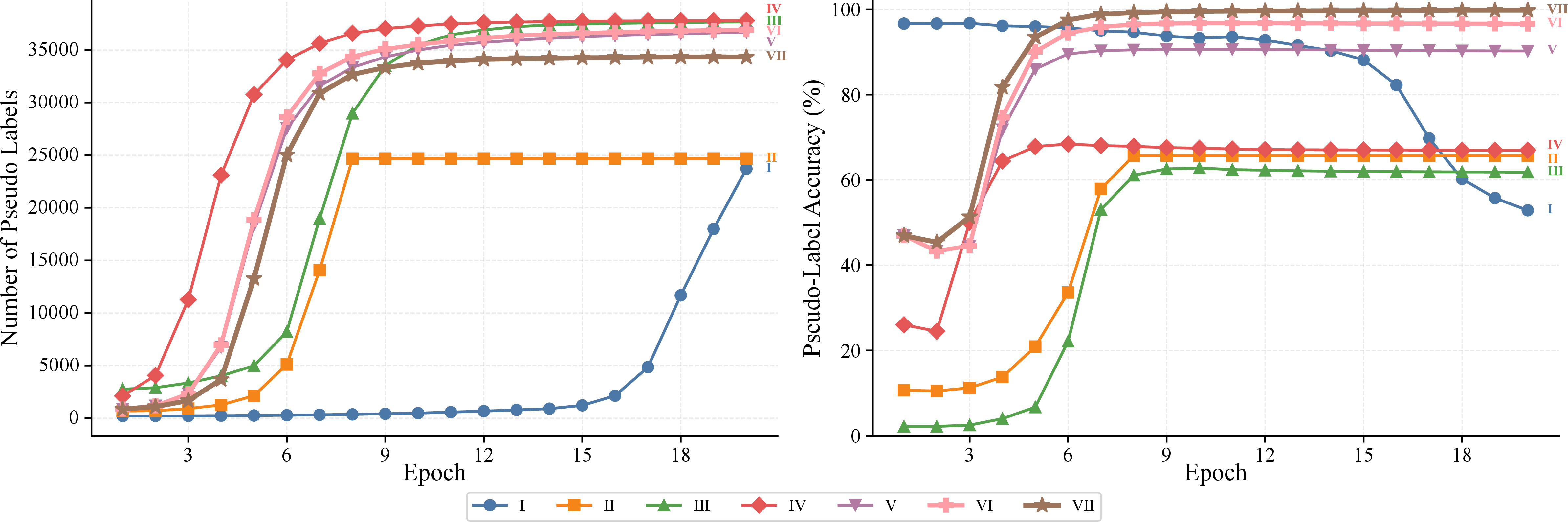
We conduct progressive ablation studies on the University-1652 dataset to evaluate the contribution of each component in STEAM. Table 3 reports the retrieval performance, while Fig. 3 illustrates the evolution of pseudo-label quantity and accuracy during training. SAFA denotes the spatial-aware feature aggregation module proposed in [7]; SSA is the proposed Stable Spatial-Aware Module, where SSA\(^*\) indicates parameter sharing between the two branches; BTSM denotes Bidirectional Top-\(K\) Soft Matching; and AdPu-U and AdPu-R denote Confidence-aware Update and Expired Label Removal, respectively.
Replacing SAFA with SSA (II\(\rightarrow\)III) substantially improves D2S R@1 from 56.46% to 74.93%. As shown in Fig. 3, SSA consistently produces more pseudo-labels with higher accuracy throughout training, indicating improved feature representation stability. Enabling parameter sharing (III\(\rightarrow\)IV) further enhances cross-view feature consistency, increasing D2S R@1 to 79.57%.
Introducing BTSM (IV\(\rightarrow\)V) yields the largest performance gain, boosting D2S R@1 by 10.98% (79.57%\(\rightarrow\)90.55%). Meanwhile, the number of pseudo-labels increases significantly while the pseudo-label accuracy remains around 90%, demonstrating that elastic matching effectively expands pseudo-label coverage without introducing excessive noise.
Applying AdPu-U (V\(\rightarrow\)VI) further improves pseudo-label quality by replacing historical labels with higher-confidence matches. Consequently, the pseudo-label accuracy increases from approximately 90% to over 96%, leading to a further improvement of D2S R@1 to 93.59%. Finally, AdPu-R (VI\(\rightarrow\)VII) removes outdated pseudo-labels that are no longer supported by the current feature space, maintaining the pseudo-label accuracy above 99% during the later training stage and achieving the best retrieval performance of 95.26% D2S R@1 and 96.01% S2D R@1.
In summary, SSA, BTSM, and AdPu are complementary: SSA provides stable feature representations, BTSM discovers high-quality pseudo-labels for cross-view matching, and AdPu maintains a reliable pseudo-label repository, together enabling effective end-to-end self-training.
4.4 Influence of \(K\) in Elastic Matching↩︎
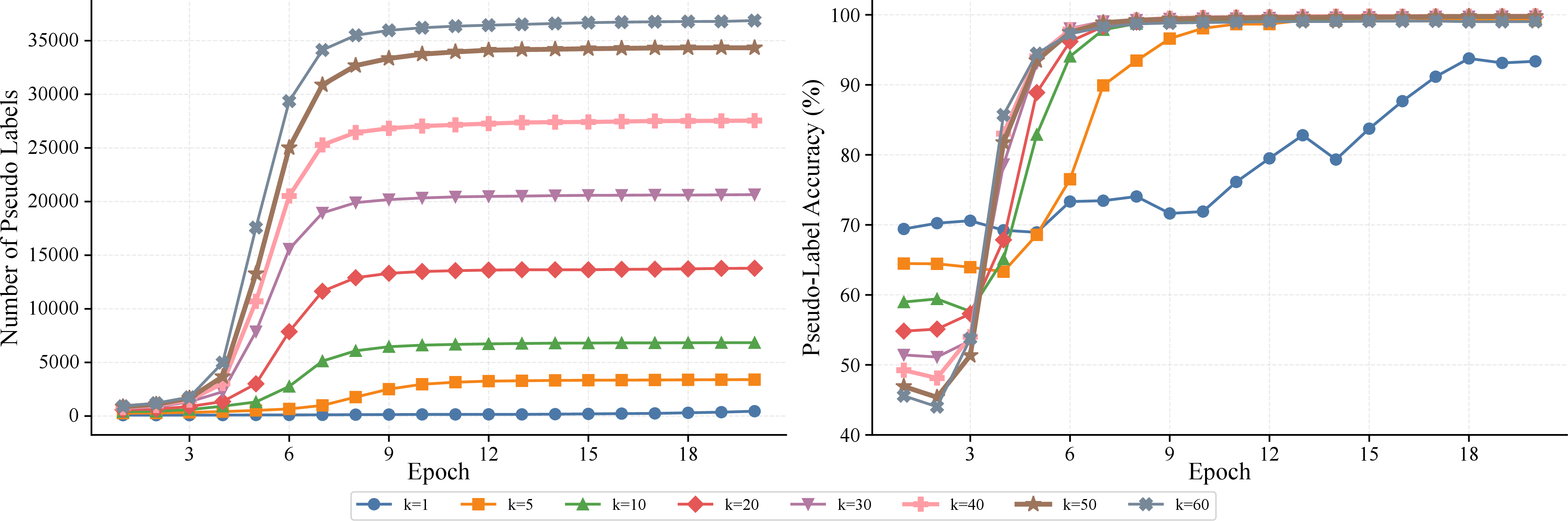
We evaluate \(K \in \{1,5,10,20,30,40,50,60\}\). Fig. 4 shows the evolution of the number of pseudo-labels and pseudo-label accuracy during training.
When \(K=1\), matching degenerates to strict mutual nearest-neighbor selection. The number of discovered pseudo-labels remains extremely low throughout training (fewer than 500 pairs after 20 epochs), while accuracy stays above 90%. As \(K\) increases, more candidate correspondences are included, leading to a substantial growth in pseudo-labels. At \(K=50\), the count reaches approximately 34,000 with accuracy as high as 99.8%, indicating that elastic matching effectively expands coverage without sacrificing label quality. Further increasing \(K\) to 60 introduces a slight drop in accuracy (around 99.0%) with only marginal growth in quantity.
In terms of retrieval performance, \(K=1\) suffers from insufficient coverage and achieves low recall, while \(K=50\) strikes the best balance between coverage and precision, yielding the highest D2S R@1. We therefore adopt \(K=50\) as the default.
4.5 Influence of \(M_e\) in Adaptive Purification↩︎
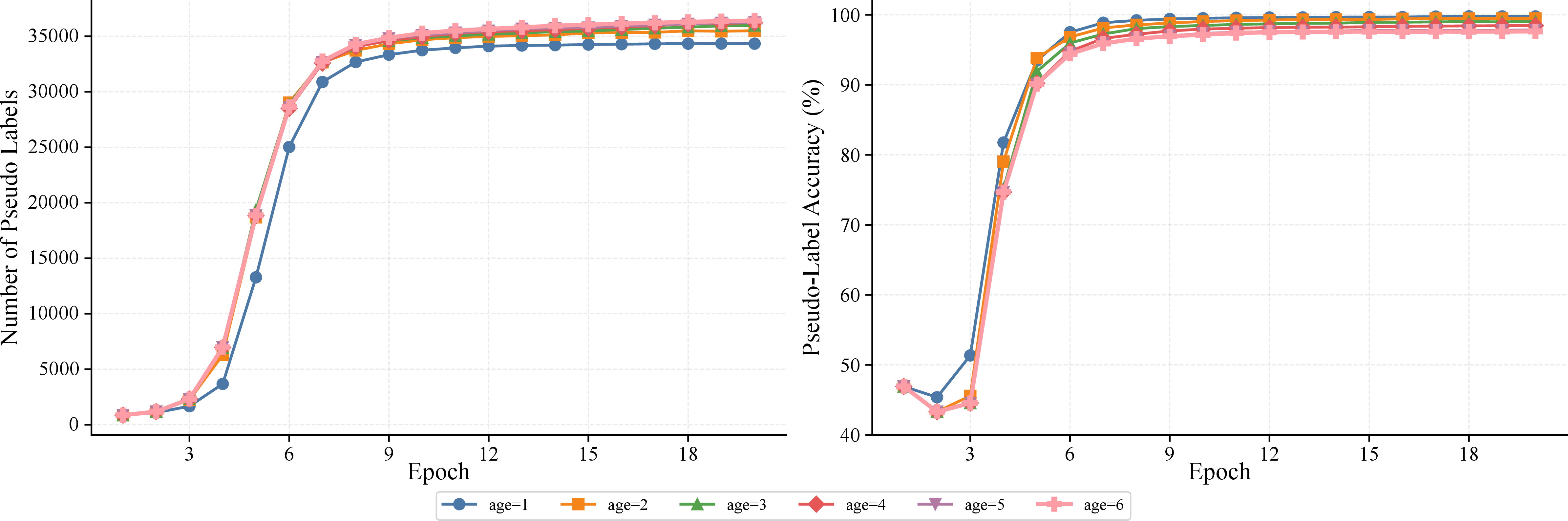
We evaluate maximum label age \(M_e \in \{1,2,3,4,5,6\}\). Fig. 5 plots the evolution of the number of pseudo-labels and pseudo-label accuracy under each setting.
With \(M_e=1\), an entry is removed immediately if not reconfirmed in the next epoch. This strategy maintains the highest pseudo-label accuracy (99.78%) with a stable count around 34,300 at epoch 20. Increasing \(M_e\) to 2 allows stale labels to persist longer: the final number of pseudo-labels rises slightly, but accuracy decreases to 99.5%, indicating that retained older labels are less reliable. For \(M_e \ge 3\), accuracy degrades more noticeably (e.g., dropping below 98.5% at \(M_e=4\)), while the quantity increase remains marginal.
These trends demonstrate that high‑quality pseudo-labels are consistently re‑discovered across consecutive epochs, while stale labels that are not reconfirmed contribute little to training and dilute the repository’s purity. Consistent with the ablation study, \(M_e=1\) achieves the best D2S R@1 by maintaining the cleanest pseudo-labels. We thus set \(M_e=1\) for all experiments.
5 Conclusion↩︎
In this paper, we propose STEAM, a unified framework for UCVGL. Unlike existing methods that rely on generative models, clustering-based initialization, or complex multi-stage optimization, STEAM enables end-to-end self-training directly on real drone and satellite images. By integrating a Stable Spatial-Aware Module, Elastic Matching, and Adaptive Purification, STEAM progressively builds reliable cross-view correspondences while effectively mitigating the accumulation and propagation of noisy pseudo-labels. Extensive experiments on two benchmark datasets demonstrate that STEAM achieves state-of-the-art performance among existing unsupervised methods, validating its effectiveness and robustness for cross-view representation learning.