1 Introduction↩︎

Discrepancy theory covers a wide array of problems and methods in combinatorics, geometry and analysis that involve approximation of a mathematical object by discrete elements [1], [2]. This field has been a long-standing focus of computer science and scientific computing, ranging from differential privacy and analog-to-digital conversion to causal inference and learning theory [3]–[8]. One of the main problems in combinatorial discrepancy is vector balancing: given vectors \(a_1,\ldots,a_k\) in a normed space, our objective is to choose signs \(\varepsilon_1,\ldots,\varepsilon_k \in \{-1,1\}\) in order to approximate the zero vector, i.e., minimize \[\begin{align} \| \varepsilon_1a_1+\ldots+\varepsilon_k a_k\|. \end{align}\] We will focus on a version of this problem posed as a zero-sum game between two players, Paul and Carol.¹ The game is played for \(T\) rounds where Paul reveals a set of \(k=n T\) vectors in \(\mathbb{R}^m\) for \(m \geq 2\) to Carol not all at once, but sequentially in \(T\) batches of size \(n\).

Since the case when \(T=1\) corresponds to the classic open problem known as the Komlós conjecture, we will refer to our game as the online Komlós game, formally defined as follows. At round \(t=0\), we initialize the vector \(y_t \in \mathbb{R}^m\) with \(y_0 = 0\). In each subsequent round from \(t= 1\) until the final round \(T\), Paul chooses \(n\) vectors \(a_{1,t},\ldots,a_{n,t} \in \mathbb{R}^m\), each with at most unit Euclidean length, and reveals them to Carol. Then Carol irrevocably chooses \(n\) signs \(\bar \varepsilon_t = (\varepsilon_{1,t},\ldots,\varepsilon_{n,t}) \in \{-1,1\}^n\), and we update \[\begin{align} y_{t} = y_{t-1}+(\varepsilon_{1,t}a_{1,t}+\ldots+ \varepsilon_{n,t}a_{n,t}). \end{align}\] We will write this update more compactly as \(y_{t} = y_{t-1} + A_t\bar \varepsilon_t\) where \(A_t\) denotes the \(m \times n\) matrix whose columns are given by the vectors \(a_{1,t},\ldots,a_{n,t}\). Paul’s objective is to make the norm \(\|y_T\|_\infty\) as large as possible, while Carol’s objective is to make it as small as possible.

Paul is referred to as an adaptive adversary because he can choose each \(A_t\) based on Carol’s choices of \(\bar \varepsilon_\tau\)’s at earlier times \(\tau <t\). Accordingly, the value \(K_{T}(m,n)\) of the online Komlós game is given by \[\begin{align} \label{e:online32Komlos} K_{T}(m,n) := \max_{A_1}\min_{\bar \varepsilon_1} \ldots \max_{A_T}\min_{\bar \varepsilon_T}\|A_1\bar \varepsilon_1+\ldots+A_T\bar \varepsilon_T\|_\infty \end{align}\tag{1}\] where the feasible set of each \(A_t\) is given by all \(m \times n\) matrices with columns of at most unit Euclidean length and each \(\bar \varepsilon_t \in \{\pm 1 \}^n\).

Kohn and Serfaty [9] established a connection between a version of this game and flow by mean curvature (see also [10]). Concretely, they found that their Paul and Carol game that is closest to ours (which they refer to as the time-dependent “inverse game"), is characterized in a continuum limit by the following nonlinear PDE \[\begin{align} \partial_tu + \max\big \{\Delta u-\big(D^2u \tfrac{\nabla u}{|\nabla u|},\tfrac{\nabla u}{|\nabla u|}\big),0\big \} = 0. \end{align}\] They also consider the continuum limit of several other games and arrive at various other PDE, such as \[\begin{align} \label{e:motion32by32mean32curvature} \partial_tu + \Delta u-\big(D^2u \tfrac{\nabla u}{|\nabla u|},\tfrac{\nabla u}{|\nabla u|}\big) = 0. \end{align}\tag{2}\] They obtain this last PDE using a game where Paul is restricted to choose batches forming orthonormal frames of \(m-1\) vectors. The equation 2 is known as the level set formulation for mean curvature flow (MCF), since the level sets of the solution \(u(\cdot,t)\) move with velocity equal to their mean curvature.

In this work we obtain a continuum limit for the online Komlós game, whose value is given by 1 . Namely, we show an analogue of the result of Kohn and Serfaty holds in our setting, when the only condition on the vectors \(a_{i,t}\) is that they all lie in the Euclidean unit ball. Accordingly, our first result shows that the leading order term of \(K_{T}(m,n)\) as \(T\to \infty\) is given in terms of the extinction time of the cube \([-1,1]^m\) under mean curvature flow. (In the interest of exposition we state here only special cases of the main theorems and defer the complete statements along with relevant definitions to Section 2.)

The complete result is recorded later in Theorem 3; it covers asymptotics for online vector balancing in any norm and batches of any size \(n\), including \(n=1\). This result opens the door to studying the asymptotics of the value function \(K_{T}(m,n)\) using tools from PDEs and geometry. Our second result characterizes how the long-time asymptotics in Theorem 1 grow with \(m\).

These estimates are based on a more general result covering centrally symmetric convex bodies, see Theorem 4 and Remark 5; they are obtained by means of comparison principle arguments, relating the solution of 2 to solutions of a linear heat equation. We believe our bounds are of interest independent of the online Komlós game. As we discuss in Section 1.3, smooth potentials, like the hyperbolic cosine and exponential weights, have been used extensively to prove upper bounds in offline and online vector balancing problems. On the other hand, our use of a potential (the heat equation solution) to establish a lower bound appears less common in this setting (one example is [11]). A similar approach has been used to establish lower bounds on regret in online learning, see for example [12]–[15].

1.1 The classic and online Komlós problems↩︎

As noted earlier, when \(T=1\), our game reduces to a classic problem, which is subject to a long-standing conjecture attributed to János Komlós [16]: \[\begin{align} \emph{The Koml\'os conjecture: } K_1(m,n) = O(1) \text{ as } m,n\to \infty. \end{align}\] Without loss of generality, it is sufficient to resolve this conjecture when \(n = m\) [17], [18]. In the 90’s, Banaszczyk established estimates for a broad class of vector balancing problems [19], [20], obtaining an \(O(\sqrt{\log m})\) upper bound for \(K_{1}(m,n)\) [20]. Paul can achieve the trivial lower bound of 1 on \(K_{1}(m,n)\) by choosing an arbitrary orthonormal set of \(m\) vectors in \(\mathbb{R}^m\), and Kunisky improved this lower bound to \(1 +\sqrt{2} -o(1)\) as \(m\) gets large [21]. In recent work, Bansal and Jiang improved on the state of the art by proving an \(\tilde{O}(\log ^{1/4} n)\) upper bound in the Komlós setting [22].²

The Komlós conjecture is a statement about the asymptotics for \(K_{T}(m,n)\) for \(T=1\) as the dimension \(m\) and number of vectors \(n\) become large, while our Theorems 1 and 2 cover the large \(T\) regime, and consider the large \(m\) and \(n\) limit only after passing to the limit in \(T\). It is an interesting possibility that the behavior of \(u(x,t)\) solving 2 with \(u(x,T) = \|x\|_\infty\) as \(t\to T\) might encode information about the offline Komlós problem. We have tried without success to find such a connection. There might be a connection, or it might be that information about \(K_{1}(m,n)\) is lost in the continuum limit.

Nonetheless, as random walk and potential-based iterative methods are used broadly in offline discrepancy problems, we hope our results will provide a helpful point of view for these methods. We also hope the PDE perspective proves helpful to other types of vector balancing problems, such as online problems with oblivious adversary or random vectors sampled from a fixed distribution. These problems are reviewed in Section 1.3.

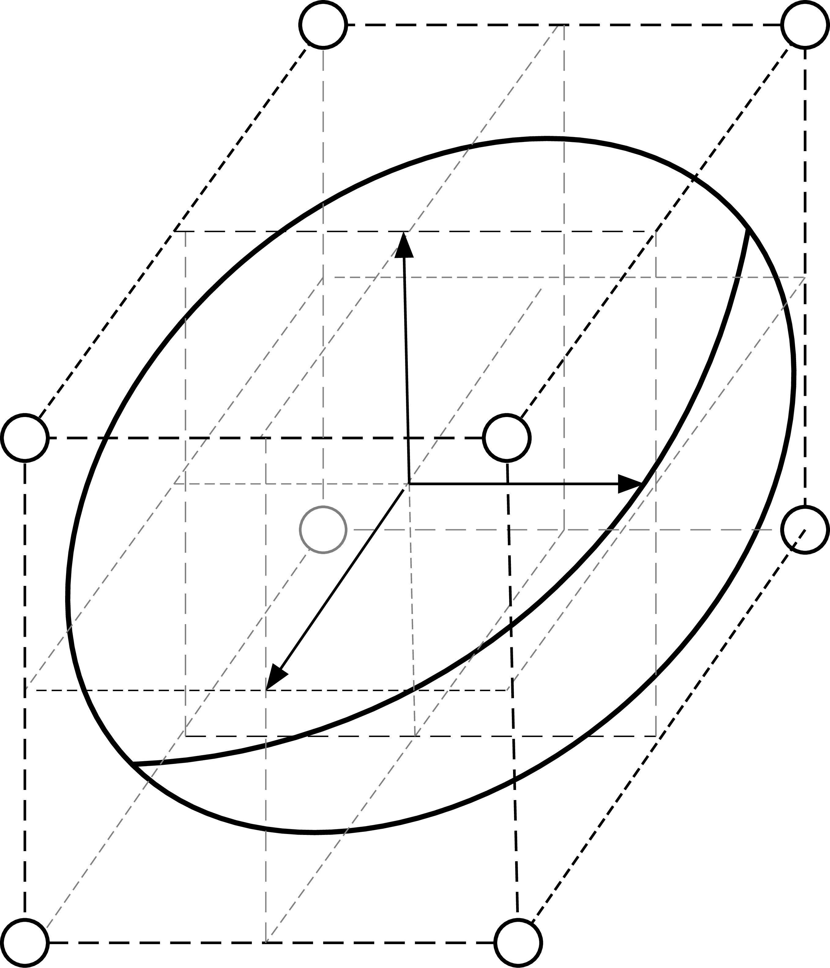
Determining the dimensional asymptotics of the “large \(T\) asymptotics” is a localization of the original Komlós conjecture, as we now explain. It will be convenient to consider the Komlós problem for a general norm \(\|\cdot\|_E\) \[\begin{align} \mathcal{K}_{n,1}(E) := \max_{A}\min_{\overline{\varepsilon}}\|A\overline{\varepsilon}\|_E, \end{align}\] where \(E\) stands for the unit ball for the norm (later, the case \(\|\cdot\|_\infty\) will be approximated by other norms). From Paul’s perspective, the classic Komlós problem consists (see Figure 1 above) in finding \(a_1,\ldots,a_n\) so that no matter what Carol chooses for \(\varepsilon_1,\ldots,\varepsilon_n\) Paul can reach, when starting from the origin, and in one step, as large as possible a multiple of \(\partial E\). As such, Paul must consider all of \(E\) in choosing \(a_1,\ldots,a_n\). Heuristically speaking, this is a global problem in \(E\).

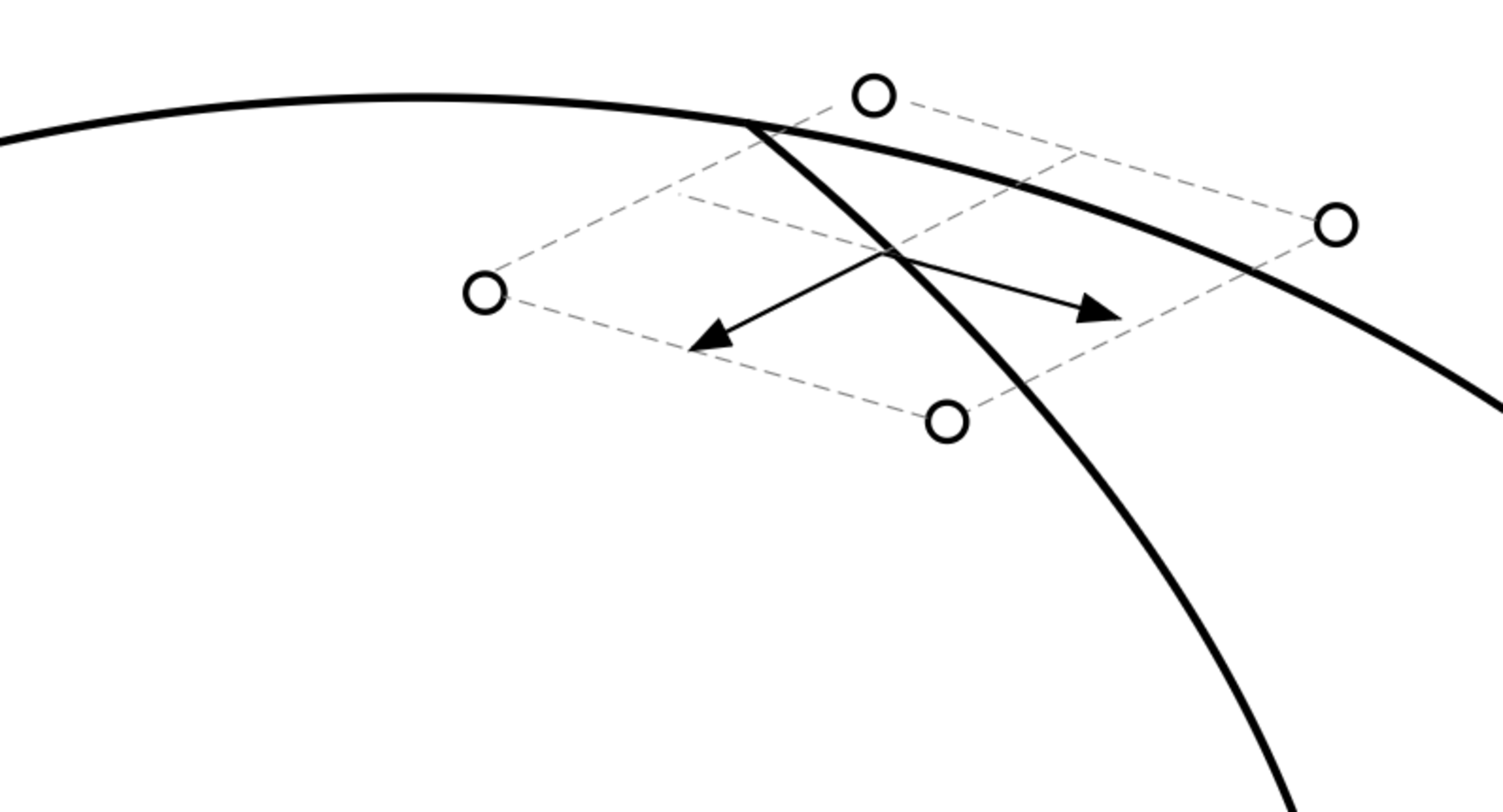
Contrast this with what happens in the online Komlós game with respect to \(\|\cdot\|_E\) after a large number of steps (see Figure 2), that is, when we are considering for a large \(T\), \[\begin{align} \mathcal{K}_{n,T}(E) := \max_{A_1}\min_{\overline{\varepsilon}_1}\ldots\max_{A_T}\min_{\overline{\varepsilon}_T}\|A_1\overline{\varepsilon}_1+\ldots+A_T\overline{\varepsilon}_T\|_E. \end{align}\] Consider a vector \(y_{T-1}\) with the property that \[\begin{align} \mathcal{K}_{n,T}(E) = \max_{A}\min_{\overline{\varepsilon}}\|y_{T-1}+A\overline{\varepsilon}\|_E, \end{align}\] in particular, we expect \(\lambda := \|y_{T-1}\|_E\) to be large when \(T\) is large (see 5 later on). In this case, Paul finds \(y_{T-1}\) placed on a large rescaling \(\lambda \partial E\) of \(\partial E\), and he is trying to reach a set \((\lambda+h) \partial E\) for as large a value of \(h>0\) as possible. However, since the columns of \(A\) have \(\ell_2\) norm at most \(1\), the available positions for Paul which are all of the form \(y_{T-1}+A\overline{\varepsilon}\) see only a relatively small region of \(\lambda \partial E\) – since we expect \(\lambda\) to be large when \(T\) is large.

Then, if \(\partial E\) is smooth, the region of \(\lambda \partial E\) immediately accessible to Paul from \(y_{T-1}\) (see Figure 2) will be approximately an ellipsoid (again, provided \(T\) and thus \(\lambda\) is large). This ellipsoid will be one passing through \(y_{T-1}\) and have the same curvature at \(y_{T-1}\) as \(\partial E\), indicating that in this regime (\(T\) large) the curvature of \(\partial E\) governs how \(\mathcal{K}_{n,T}(E)\) is changing with \(T\). This heuristic picture is discussed further in Section 3.

1.2 Notation↩︎

For a vector \(x\) in \(\mathbb{R}^n\), \(\|x \|_p\) denotes its \(\ell_p\) norm, and \(|x |:=\|x\|_2\) specifically denotes the Euclidean (\(\ell_2\)) norm. For vectors \(x\) and \(y\) in \(\mathbb{R}^m\), \((x, y)\) denotes their Euclidean inner product. The vector \(e_i\) represents the \(i\)-th canonical basis vector of \(\mathbb{R}^m\). Given a centrally symmetric body \(E \subset \mathbb{R}^m\), \(\|\cdot\|_E\) denotes the unique norm in \(\mathbb{R}^m\) whose unit ball is equal to \(E\). Its dual norm \(\| \cdot\|^*_E\) is given by \(\|z\|^*_E:= \sup_{\| y\|_E\leq 1} ( z, y )\). For a matrix \(M \in \mathbb{R}^{m \times m}\), its operator norm is denoted by \(\|M\|\). Finally, the discrepancy of a matrix \(A \in \mathbb{R}^{m \times n}\) is defined as \[\text{disc}(A) :=\min_{\bar \varepsilon\in \{ \pm 1\}^n } \|A \bar \varepsilon\|_ \infty.\]

1.3 Previous work on vector balancing↩︎

The taxonomy of vector balancing problems is based on two primary characteristics. The first one specifies how the vectors are chosen. When Paul chooses vectors adversarially, as in our game, this setting is called the worst-case discrepancy. On the other hand, the average case discrepancy refers to the setting when the vectors are sampled independently from a distribution known to Carol. The second primary characteristic specifies when the vectors are revealed to Carol: in the offline setting Paul reveals all of them before Carol chooses any signs, while in the online setting, Paul reveals the vectors one-by-one and Carol irrevocably chooses the sign of each vector revealed in a given period, before the next vector is revealed [23]. Our online Komlós game interpolates between the purely online setting when Paul reveals one vector at a time and is the strongest adversary (\(n=1\)), and the purely offline setting when Paul reveals all vectors at once and is the weakest adversary (\(T=1\)).

Offline and online vector balancing problems have been studied in large part using randomized and/or potential-based iterative methods. Since it is plausible that some of these problems may be analyzed using PDE-based methods, we will now review some of the previous work on vector balancing, highlighting connections to those iterative methods. Due to space limits, we could not survey all potentially relevant recent discrepancy problems, such as Gaussian discrepancy [24], online geometric and interval discrepancy [11], [25], bad science matrices [26]–[28], or matrix discrepancy [29]–[31]. We refer the reader to the ICM survey by Bansal for a more comprehensive and in-depth treatment of discrepancy theory and related algorithms [32].

Offline worst case. One of the classic discrepancy minimization problems entails coloring the elements of a set \(U\) of size \(n\) with binary colors \(\{\pm 1\}^n\) so that each member of a given collection of \(m\) subsets of \(U\) is colored in the most balanced way possible. This collection can be represented by the incidence matrix \(A \in \{0,1\}^{m\times n}\), and the balance of coloring is measured by \(\text{disc}(A)\). For a closely related class of matrices: \(A \in \mathbb{R}^{m \times n }\) and all \(|A_{ij}|\leq 1\) (we will refer to this setting as the set coloring), Spencer established that \[\text{disc (A)} =O \big(\sqrt {n \log( 2m /n) }\big)\]by a partial coloring method using the binary entropy potential [16]. This result was also obtained by Gluskin using a different method also based on partial coloring [33], and Giannopoulos provided a simplified version of Gluskin’s proof [34]. When \(n \geq m\), this upper bound can be taken to be \(5.32 \sqrt {m}\), which led to its memorable “six standard deviations suffice" characterization. (Pesenti and Vladu [35] improved the constant prefactor in the set discrepancy setting from 5.32 to 3.68.) A matching \(\Omega (\sqrt{m})\) lower bound in this setting is achieved by Hadamard matrices [3], [36].

Spencer also showed that if Carol can delete a constant fraction of vectors, i.e., set their colors to zero, then the Komlós conjecture holds for this modified problem[16]. Bandeira, Maillard and Zhivotovskiy [37] provided an alternative proof of this result based on the partial coloring theorem of Kashin [38], and yet another earlier proof of this result was given by Lonke [39]. On the other hand, Chasapis and Skarmogiannis showed that if Carol is prevented from using all possible colorings, specifically if the feasible set of \(\bar \varepsilon\) is \(S \subset \{\pm 1 \}^m\) has at most \(2^{\delta n}\) colorings for \(\delta \in (1/m, 1)\), then the discrepancy in this modified problem is lower bounded as \(\Omega \big(\sqrt{\log(e/\delta)}\big)\) [40], and Hajela established a similar result earlier [41]. Recently, Smirnov and Vershynin gave a Fisher information perspective on partial coloring based on the first Dirichlet eigenvalue of the hypercube [42].

Bansal developed the first polynomial-time algorithm for partial coloring that achieves Spencer’s upper bound using a random walk with covariance determined by semidefinite programming (SDP)[43]. Subsequently, Lovett and Meka developed a simpler algorithm that achieved the same upper bound using a random walk inside the unit hypercube in a polytope \(\mathbb{R}^m\) with certain discrepancy constraints [44]. Rothvoss, as well as Eldan and Singh, developed partial coloring algorithms that generalize to symmetric convex bodies beyond polytopes [45], [46]. Charikar, Newman, and Nikolov established that it is NP-hard to distinguish between set systems with discrepancy zero and \(\Omega(\sqrt {m})\); thus we do not expect to be able to efficiently find an optimal coloring for set systems with an \(o(\sqrt {m})\) discrepancy [47]. On the other hand, a closely related quantity called hereditary discrepancy of a matrix \(A\), or \(\text{heredisc}(A)\), that upper bounds \(\text{disc} (A)\), can be efficiently approximated [48].

Bansal, Dadush, and Garg developed the first efficient algorithm based on a random walk with covariance determined by an SDP solution that achieved Banaszczyk’s upper bound in the Komlós setting [49]. Levy, Ramadas and Rothvoss developed a deterministic algorithm based on the multiplicative weights potential that achieved this upper bound; this algorithm also achieves the \(O(\sqrt {m})\) bound in the set discrepancy setting [50]. Subsequently, Bansal, Dadush, Garg and Lovett developed an algorithm that achieves Banaszczyk’s bound for vector balancing in general convex bodies; their algorithm is based on a random walk that evolves in directions obtained by the Gram-Schmidt process [51]. Harshaw, Sävje, Spielman, and Zhang improved the variance bounds of the signed vectors sums obtained in this process [7], and Bednorz and Godlewski used this Gram-Schmidt walk to improve (i) the constant prefactor in Banaszczyk’s \(O(\sqrt {\log m})\) upper bound in the Komlós setting and (ii) the discrepancy bounds in the smoothed analysis of the Komlós conjecture with Gaussian noise (this setting is further discussed below)[52]. Lastly, Bansal, Laddha and Vempala gave a deterministic algorithm based on a time-dependent barrier function that achieves all the bounds described above – Spencer’s set coloring bound \(O \big(\sqrt {n \log( 2m /n) }\big)\), Banaszczyk’s upper bounds in the Komlós setting – as well as certain bounds in the spectral hypergraph and Gaussian random matrix settings [53].

Bansal, Jiang, Meka, Singla and Sinha applied the smoothed analysis of Spielman and Teng [54] to show that the Komlós conjecture holds asymptotically almost surely (a.a.s.) when \(n= \omega(m \log m)\) and \(A\) is perturbed by adding small Gaussian noise [55] (see also [56] for the smoothed analysis of the prefix discrepancy). Aigner-Horev, Hefetz and Trushkin established a similar result when \(A\) is perturbed by Rademacher noise [57].

Offline average case. While the Komlós conjecture remained unresolved, a substantial amount of work was dedicated to estimating discrepancy of special classes of random and pseudorandom matrices. For Gaussian matrices \(A \in \mathbb{R}^{m \times n}\) with each \(A_{ij} \sim N(0,1)\) independently, Costello established that \(\text{disc}(A) = \Theta (2^{-n/m}\sqrt{n})\) a.a.s. when \(m\) is fixed [58], and Turner, Meka and Rigollet established the same result when \(\omega(1) = m =o(n)\) [59].³ In the Gaussian matrix setting, Chandrasekaran and Vempala upper bounded discrepancy as \(O(\sqrt {n \log (m/n)})\), modulo a polylog term in \(m\) and \(n\), when \(2n \leq m \leq 2^n\) [60]. Pesenti and Vladu gave an algorithm based on the Stieltjes regularizer of the max function that was used to prove the Komlós conjecture for certain pseudorandom matrices, as well as for random orthogonal and random Gaussian matrices [35].

In the discrete random matrix setting, Ezra and Lovett showed that when the columns of \(A\in \mathbb{R}^{m \times n}\) are sampled from \(s\)-sparse vectors in \(\{0,1\}^m\) uniformly and \(m \geq n \geq s\), \(\text{heredisc}(A) = O(\sqrt {s \log s})\) and when \(n \gg m^s\), \(\text{heredisc}(A) = O(1)\) with high probability [61]. Hoberg and Rothvoss showed \(\text{disc}(A) \leq 1\) with high probability when \(A_{ij} \sim \text{Bernoulli}(p)\) independently provided that \(n = \Omega (m^2 \log m)\) and \(mp = \Omega (\log n)\) [62]. Franks and Saks showed that \(\text{disc}(A) \leq 2\) with high probability for a rather broad class of random \(s\)-sparse matrices when \(n = \Omega (m^3 \log^2 m)\) [63]. Altschuler and Niles-Weed showed \(\text{disc}(A) = O(1)\) with high probability when \(A_{ij} \sim \text{Bernoulli}(p)\) independently and \(n \geq C m \log m\) where \(p\) may be varying with \(n\); they also provided a discrepancy upper bound for a broad class of Poisson random matrices [64].

Online worst case with adaptive adversary. As noted earlier, in the context of online discrepancy, Paul is called an adaptive adversary whenever he is able to choose the vectors based on Carol’s choices of signs at earlier times. Spencer showed that in the online version of the set discrepancy problem, where Paul chooses \(a_t\) with \(\|a_t\|_\infty \leq 1\) adaptively, the discrepancy is \(\Theta (\sqrt {T \log T})\); the upper bound is established using the \(\cosh\) potential, while the lower bound is established by analyzing the distribution of certain hitting times of a one-dimensional random walk [18] (see also [65]). Haghtalab, Roughgarden and Shetty gave an algorithm that guarantees an \(\tilde{O}(\log^2(mT/\sigma))\) upper bound on discrepancy in a modified version of our online Komlós game with \(n=1\) where the adversary selects the vectors from an adaptive \(\sigma\)-smooth isotropic distribution where density is upper bounded pointwise by \(1/\sigma\) times the density of the uniform distribution. Their algorithm uses the \(\cosh\)-based potential introduced by Bansal, Jiang, Meka, Singla and Sinha in the online average case discussed below [66], [67]. Without smoothing our online Komlós game with \(n=1\) appears trivial: by equation 5 , \[1/\sqrt{2} \leq K_{t}(m,1)/\sqrt{t} \leq 1,\] uniformly in \(m\) (see also the discussion of Game 1 in [23]). Perhaps due to this, much of the recent online vector discrepancy literature focused on the average case discrepancy, as well as adversaries that are not adaptive, the so-called oblivious adversaries.

Online average case. When the vectors are sampled from the uniform distribution over \(\{\pm 1\}^m\) independently and revealed to Carol online, Bansal and Spencer gave a strategy based on an inverse polynomial potential that guarantees with high probability an \(O (\sqrt {m})\) discrepancy, as well as another strategy based on the \(\cosh\) potential that guarantees an \(O (\sqrt {m } \log m)\) prefix discrepancy [68] (the prefix discrepancy controls the \(\ell_\infty\) norm of the partial sums \(y_t\) uniformly across time, not just at the final time). When the vectors are sampled independently from an arbitrary distribution over \([-1,1]^m\) with potentially non-independent entries, Bansal, Jiang, Singla and Sinha gave an \(O(m^2( \log T + \log m))\) online prefix discrepancy bound using the \(\cosh\) potential [11]. Improving on this result, Bansal, Jiang, Meka, Singla and Sinha gave an \(O( \log^4 (mT))\) bound on online prefix discrepancy when vectors are sampled independently from an arbitrary distribution on the unit \(\ell_2\) ball in \(\mathbb{R}^m\) [67].

A special case of the Komlós conjecture is the Beck-Fiala conjecture: for any \(A \in \{0,1\}^{m\times n}\) with column sparsity of at most \(s\), \(\text{disc}(A) = O(\sqrt {s})\)[17]. In this setting, Altschuler and Tikhomirov established that there exists an asymptotic gap between the discrepancy in the online and offline vector balancing of independent uniformly random \(s\)-sparse vectors [69]. Finally, when the vectors are sampled independently from the standard \(m\)-dimensional Gaussian and revealed to Carol online, Fiedler, Jackson, Lacker and Niles-Weed established a \(\Theta (\sqrt {m})\) discrepancy estimate in expectation; their lower bound applies more generally to all random vectors with i.i.d. mean zero and variance 1 entries with finite fourth moments[70]. Although their methods are grounded in mean-field stochastic control, their use of a discrete value function defined by dynamic programming is similar to ours.

Online worst case with oblivious adversary. In the oblivious setting, Paul still reveals the vectors to Carol sequentially. However, he cannot use Carol’s earlier choices of signs when he selects a vector in a given round. Since every deterministic algorithm for choosing signs has the same worst case discrepancy against an oblivious adversary as against the corresponding adaptive adversary (whenever the oblivious adversary correctly guesses the worst case pattern of vectors in the adaptive case) Carol is permitted to use randomized policies, and the discrepancy is evaluated with high probability with respect to Carol’s randomization.

In the online Komlós setting with an oblivious adversary, Kulkarni, Reis and Rothvoss achieved the state-of-the-art \(O \big (\sqrt {\log (\min (m,T))}\big )\) discrepancy upper bound and \(\Theta \big (\sqrt {\log T})\) prefix discrepancy upper and lower bounds, modulo a term that depends on the probability of attaining this bound[71]. Their upper bound strategy depends on the entire series vectors \(a_1, \dots a_{t-1}\) (and therefore does not appear to be Markovian). Earlier, Alweiss, Liu and Sawhney achieved an \(O(\log mT)\) prefix discrepancy bound with high probability using a "self-balancing random walk" algorithm that is Markovian - it depends on the current time \(t\) and the inner product of the partial sum \(\sum_{\tau=1}^{t-1} \varepsilon_{\tau} a_{\tau}\) with the vector \(a_t\) revealed to Carol in the current period [72].

1.4 Mean curvature flow and the level set PDE↩︎

The nonlinear PDE 2 is known as the level set formulation of mean curvature flow, and it is one of several alternative descriptions of this geometric evolution. The mean curvature flow appears in many areas of pure and applied mathematics, receiving thorough and complementary treatments from the perspectives of geometric measure theory [73], [74], the theory of nonlinear parabolic equations [75]–[77], and geometric analysis [78], among others.

Brakke’s mean curvature flow. The mean curvature flow was introduced by Brakke in his doctoral dissertation [73], and accordingly sometimes it is known as Brakke’s mean curvature flow. Informally speaking, a time-evolving family of closed hypersurfaces \(S_t \subset \mathbb{R}^m\) (enclosing domains \(E_t\), so \(S_t = \partial E_t\)) is said to be evolving by mean curvature flow if the inner normal velocity of \(S_t\) at any point \(p\in S_t\) is equal to the sum of the principal curvatures of \(S_t\) at \(p\).

The informal description above masks a number of deep analytical and geometrical difficulties revolving around the right definition of such a flow, and the nature of the singularities that may form over time even if one starts the flow from a smooth hypersurface. Brakke’s original work [73] falls within the framework of geometric measure theory, working with varifolds to formulate a notion of solution for this flow. For a modern treatment of the mean curvature flow from this perspective, see Tonegawa’s monograph [74].

Huisken’s theorem and extinction times. A celebrated Theorem of Huisken [79] says that if the initial surface \(S_0\) is the boundary of a convex body \(E_0\), then the surface remains convex for the duration of the mean curvature flow. To be exact, Huisken showed there is a positive time \(\tau = \tau(E_0)\) and a mean curvature flow \(S_t\) defined for \(t\in [0,\tau)\) and starting from \(S_0\), and such that \(S_t\) is the boundary of a smooth convex set for every \(t\in (0,\tau)\), and that \(S_t\to \{x_*\}\) in the Hausdorff topology to some point \(x_* \in \mathbb{R}^m\).

In Huisken’s work the flow is represented via a map \(F:\mathbb{S}^{m-1}\times [0,\tau) \to \mathbb{R}^m\) such that \(F(\cdot,t)\) gives a parametrization of \(S_t\), the evolution of the map \(F(\cdot,t)\) with \(t\) is governed by a nonlinear parabolic equation for the map \(F\). As \(t\to \tau\), the map \(F(\cdot,\tau)\) converges to a constant (i.e. to the point to which the surfaces are shrinking to as \(t\to \tau\)). The time \(\tau\) is known as the extinction time of \(S_0\), or equivalently, of \(E_0\) (see also 4 ). It defines a functional over the set of convex bodies. In general, there is no explicit expression for the extinction time \(\tau(E)\) for a given convex body \(E\) (a notable exception is a ball). We note that work of Giga and Yama-uchi [80] provides an estimate for the extinction time in terms of the Cheeger constant of \(E\), which is a fundamental quantity in geometry related to the spectral gap of the Laplace-Beltrami operator [81].⁴

The level set formulation. Level set formulations are a way of describing hypersurfaces \(S\) of \(\mathbb{R}^m\) in terms of a scalar function \(u\), “the level set function”, such that \(S = \{u=0\}\). In this way, one can describe geometric quantities of \(S\) in terms of an expression involving \(u\). For instance, if \(x\in S\), then the normal vectors to \(S\) are given by \(\pm \nabla u / |\nabla u|\). Note also that a family of hypersurfaces \(S_t\) varying in time can be represented by a time-dependent level set function \(u(x,t)\). For a general introduction to the level set method, see the book by Giga [83] and the book by Fedkiw and Osher [84].

A standard computation shows that if \(u(x,t)\) is a smooth level set function and \(\nabla u \neq 0\), then for each \(\lambda\) the level set \(S_t(\lambda) = \{ x : u(x,t) = \lambda\} = \partial \{ x: u(x,t)<\lambda \}\) is evolving in time with an inner normal velocity \(V\) at \(x \in S_t(\lambda)\) given by \[\begin{align} \label{e:level32set32velocity} V = \frac{\partial_t u}{|\nabla u|}. \end{align}\tag{3}\] This brings us to level set equations which are also parabolic⁵ PDEs. These are equations of the form \[\begin{align} \partial_t u + |\nabla u|F(D^2u,\nabla u) = 0, \end{align}\] where \(F(D^2u,\nabla u)\) is a degenerate parabolic operator, meaning that for a fixed \(p\) we have \(F(M,p) \leq F(M',p)\) whenever \(M'-M\) is a positive semi-definite matrix. In light of the formula 3 , the significance of the parabolic PDE for \(u\) is that its level sets are moving with normal velocity equal to \(F(D^2u(x),\nabla u(x))\). The level set equation is in addition called geometric if \(F(M,p) = F(M+s p\otimes p,p)\) for every \(M\), \(p\neq 0\), and \(s\in\mathbb{R}\). This means that the value of \(F(D^2u(x),\nabla u(x))\) at some \(x=x_0\) is determined by the shape of the level set of \(\{ u = u(x_0)\}\).

As an important example, the operator \(F\) giving the level set formulation of mean curvature flow is \[\begin{align} F(D^2u,\nabla u) = \mathop{\mathrm{\mathrm\mathrm{tr}}}(\Pi(\nabla u)(D^2u)\Pi(\nabla u))/|\nabla u| = \mathop{\mathrm{div}}\big( \tfrac{\nabla u}{|\nabla u|}\big), \end{align}\] where for \(p\neq 0\), \(\Pi(p)\) denotes the \(m\times m\) matrix representing the orthogonal projection onto the hyperplane normal to \(p\). This matrix is given by \((\Pi(p))_{ij} = \delta_{ij}-|p|^{-2}p_ip_j\). Then, the level set PDE for mean curvature flow is \[\begin{align} \partial_t u + |\nabla u|\mathop{\mathrm{div}}\big(\tfrac{\nabla u}{|\nabla u|}\big) = 0. \end{align}\] These equations are fully nonlinear parabolic equations, and so they fall within the scope of the theory of viscosity solutions. The level set formulation was first studied by Evans and Spruck [75] and Chen, Giga, and Goto [76]. We also mention work of Giga, Goto, Ishii, and Sato [77] dealing with general flows and which will also be essential here. As discussed earlier, Kohn and Serfaty [9] found the level set PDE for mean curvature flow arises as a continuum limit in vector balancing games. Kohn and Serfaty subsequently extended the deterministic games framework to general fully nonlinear parabolic and elliptic equations [85], and Imbert and Serfaty extended it to include integral curvature flows [86]. Concurrently, work of Peres, Schramm, Sheffield, and Wilson [87] touched on parallel themes as they established a relationship between tug-of-war games and the infinity Laplacian. There is a \(1\)-parameter family of problems connecting the infinity Laplacian [87] and mean curvature flow [9]: they are two extremes in the class of evolution \(p\)-Laplacian equations (\(p\in [1,\infty]\)). We also mention works of Charro, García Azorero, and Rossi [88], as well of Gonzalvez, Miranda, Rossi, and Ruiz-Cases [89] involving two-player zero-sum probabilistic games.

More general flows. One may evolve \(S_t = \partial E_t\) according to some other function of the principal curvatures of \(S_t\), leading to parabolic level set PDEs as above, as well as to PDE’s for maps \(F:\mathbb{S}^{m-1}\to\mathbb{R}^m\) in the smooth setting. We mention in particular work of Andrews [90], which considered general geometric flows starting from convex initial data. An important result in [90] is the preservation of convexity under natural structural assumptions on the flow (i.e. structural assumptions on the function of principal curvatures used). This is important in defining extinction times for other flows besides mean curvature.

One possibility is the flow where the normal velocity equals the sum of the largest \(n\wedge (m-1)\) principal curvatures of \(S_t\). The resulting evolution also produces a family of convex bodies that shrink down to a point at some finite time \(\tau_{n}(K)\). When \(n\geq m-1\) this is the usual mean curvature flow, and when \(n<m-1\) we refer to this as flow by the largest \(n\) principal curvatures. Flows with \(n=1\) have been shown to arise in stochastic control problems [91] (see next paragraph).

Stochastic optimization interpretation. Prior to Kohn and Serfaty’s deterministic game setting, various works showed mean curvature flow captures the reachability set for certain stochastic control problems. We mention here the works of Soner and Touzi [92], [93], of Buckdahn, Cardaliaguet, and Quincampoix [94]. More recently, Larsson and Ruf [91] found that flow by the minimum curvature describes the largest (deterministic) amount of time that a certain martingale can be kept inside a given convex body.

Viscosity solutions and fully nonlinear equations. Viscosity solutions are a powerful tool when dealing with value functions for games or control problems involving in continuum settings. As we have known since works of Bellman[95] and Pontryagin [96], a sufficiently smooth value function will solve a PDE associated to the problem, the Hamilton-Jacobi-Bellman equation. However, value functions are typically not smooth everywhere, and one must deal with generalized solutions. Among several notions of “weak solutions” to such nonlinear equations, viscosity solutions stand out for producing a complete theory of existence and uniqueness, and for correctly characterizing the weak formulation of the PDE for non-smooth value functions. Just as important is the role of viscosity solutions in the context of continuous limits, where we have Barles and Souganidis [97] celebrated theorem on the convergence of finite difference schemes to the unique viscosity solution of a PDE.

Viscosity solutions are built around a natural monotonicity property of the nonlinear operator, and which is directly related to the maximum principle. This monotonicity, sometimes known as the Global Comparison Property (GCP), imposes severe restrictions on the class of operators. In particular, Courrège showed that a linear operator in \(\mathbb{R}^n\) satisfying the GCP is essentially the infinitesimal generator of a Markov process [98]. The corresponding result for nonlinear operators was obtained by Guillen and Schwab [99], [100], where they show that a nonlinear operator having the GCP can be expressed as a min-max of linear operators of the type obtained by Courrège.

For monographs on viscosity solutions we recommend the book of Fleming and Soner [101] and the book of Bardi and Capuzzo-Dolcetta [102], both of which also cover the perspective from optimal control. We also recommend the lecture notes by Silvestre [103] as well as lecture notes by Calder [104]. Last but not least we mention the forthcoming monograph by Giga and Liu [105], which covers geometric evolution equations arising from deterministic discrete two-person games.

2 Statement of the main results↩︎

In this section, we state the main results of this paper in full generality, containing each of the special theorems discussed in the Introduction (Section 1). For the rest of the paper \(E\) will denote a centrally symmetric convex body in \(\mathbb{R}^m\), \(m\geq 2\). This body defines a norm, which we denote by \(\|\cdot\|_E\). Now, for any \(T,n \in \mathbb{N}\) we define a functional over such convex bodies by \[\begin{align} \mathcal{K}_{n,T}(E) := \max_{A_1}\min_{\overline{\varepsilon}_1}\ldots \max_{A_T}\min_{\overline{\varepsilon}_T}\|A_1\overline{\varepsilon}_1+\ldots+A_T\overline{\varepsilon}_T\|_E, \end{align}\] where for each \(t=1\ldots,T\), the minimum is taken over all \(\overline{\varepsilon}_s \in \{-1,1\}^n\) and the maximum is taken over all \(m\times n\) matrices \(A\) whose columns have at most unit Euclidean length each.

As discussed in the introduction, given \(E\) and \(n\geq 1\), there is well defined flow \(E_t\) at least for small positive times, \(E_0 = E\) and \(\partial E_t\) moves with normal velocity equal to the sum of the largest \(n\wedge (m-1)\) principal curvatures of \(\partial E_t\). The sets \(E_t\) are all centrally symmetric convex bodies and the flow is defined up until some maximum interval of existence. Then, we define the extinction time for \(E\) with respect to the flow by \[\begin{align} \label{e:extinction32time32functional} \tau_n(E) := \sup\, \Big\{ t \Bigm| \begin{tabular}{l} There exists a flow starting from E with normal velocity equal to the sum of \\ the largest n\wedge (m-1) principal curvatures, and it is non-vanishing in (0,t). \end{tabular} \Big \}. \end{align}\tag{4}\] For such a time, it is known that \(E_t \to \{0\}\) in the Hausdorff distance as \(t\to \tau_n(E)\).

The foregoing theorems are proved in Sections 6 and 7. The next section provides heuristics and overview of the proofs, while Sections 4 and 5 as well as the Appendices set forth definition and results used in the proof of Theorem 3 in Section 6.

3 Heuristics and overview of the proofs↩︎

The connection between Spencer’s pusher-chooser game and mean curvature flow was first made clear in Kohn and Serfaty’s work [9]. In their setting, Paul chooses an orthonormal frame of \(m-1\) vectors. This already produces mean curvature flow in the limit. Here we show for the same continuum limit holds when the constraint is that the vectors lie in the Euclidean unit ball (and in particular one can take any \(n\geq m\) vectors). Ultimately, this is made possible by an estimate of Banaszczyk for discrepancy with respect to the \(\ell^2\) norm [110].

Elementary strategies. To explain in rough terms the appearance of mean curvature, it helps to discuss some elementary strategies for Paul and Carol, which guarantee the following bounds at all \(T\): \[\begin{align} \label{e:intro32value32function32bound} \sqrt{ c(m,n) T} \leq K_{T}(m,n) \leq \sqrt {\min(n,m)\, T} \end{align}\tag{5}\] where \(c(m,n) := \min(n,m-1)/(\min(n,m-1)+1)\).

A possible strategy for Paul is to choose the columns of \(a_{t,1},\dots, a_{t,n^*}\) to be \(n^*:=\min(n,m-1)\) orthonormal vectors that are orthogonal to \(y_{t-1}\) in a \(n^*+1\) coordinate subspace of \(\mathbb{R}^m\) that stays fixed during the game, e.g., \(\text{span} \{e_1,\dots, e_{n^*+1}\}\), and set any remaining vectors to zero. This choice means that regardless of Carol’s choice of signs, \[\begin{align} |\varepsilon_{t,1}a_{t,1}+\ldots+\varepsilon_{t,n}a_{t,n}|^2 = |\varepsilon_{t,1}a_{t,1}|^2+\ldots+|\varepsilon_{t,n}a_{t,n}|^2 = n^*. \end{align}\] (As a reminder, in our notation, \(|\cdot |\) refers to the \(\ell_2\) norm.) Therefore, Paul can make sure that \(|y_t|^2 = |y_{t-1}|^2 + n^*\) at every step \(t\), and thus \[\begin{align} |y_t|^2 = t \, n^*,\;\forall\;t. \end{align}\] Since \(|y_t| \leq \sqrt{n^*+1}\,\|y_t\|_\infty\), one concludes that \[\begin{align} \|y_t\|_\infty \geq \sqrt{c(m,n)t}, \;\forall\;t,\;c(m,n) = n^*/(n^*+1). \end{align}\] Thanks to Banaszczyk’s theorem (see Theorem 11), whatever Paul chooses for the vectors \(a_{t,1},\ldots,a_{t,n}\), there exists a choice of signs \(\varepsilon_t\) for Carol such that \[\begin{align} |\varepsilon_{t,1}a_{t,1}+\ldots\varepsilon_{t,n}a_{t,n}|^2 \leq m. \end{align}\] On the other hand, when the signs \(\varepsilon_{i,t}\) are independently sampled uniformly at random, the expected value \(\mathbb{E}| y_t |^2 \leq n t\), and by the monotonicity of the \(\ell_p\) norm, \(\mathbb{E}\| y_t \|_\infty \leq \sqrt {n t}\). Therefore, by a probabilistic argument, there exists a deterministic policy of choosing \(\varepsilon_t\) so that \[\begin{align} |y_{t}|^2 \leq |y_{t-1}|^2 + \min(m,n), \Rightarrow \|y_t\|_\infty \leq \sqrt{t\min(m,n)}. \end{align}\] These strategies guarantee the bounds in 5 .

Appearance of the mean curvature. There is a sort of generalization of the above argument for a non Euclidean norm, and it serves to illustrate the emergence of the mean curvature in the vector balancing context. Instead of the norm \(\|\cdot\|_\infty\) let us consider a general norm \(\|\cdot\|\) whose unit ball \(E\) is assumed to be smooth.

Observe that \(y \mapsto \|y\|^2\) is a \(2\)-homogeneous function, which is smooth away from \(0\), and in particular, the second derivatives of \(\|\cdot\|\) are \(0\)-homogeneous and their third derivatives are negatively homogeneous. This means that if \(y_{t-1}\) is very large we expect \(\|\cdot\|^2\) to be close to its second Taylor expansion in say, a ball of radius \(1\) centered at \(y_{t-1}\).

Then let us assume \(\|y_{t-1}\|\) is large (as will be the case when \(t\) is large), and consider the unit vector \(\hat{y}_{t-1} :=y_{t-1} /\|y_{t-1}\|\) as well as the outer normal vector \(n (\hat{y}_{t-1})\) at \(\hat{y}_{t-1}\), which lies on \(\partial E\) with unit dual norm \(\|n (\hat{y}_{t-1})\|^* =1\). Using Euler’s identity for 1-homogeneous functions, one can check that \[\begin{align} \nabla \|\cdot\|^2 (y_{t-1}) = 2\|y_{t-1}\|n(\hat{y}_{t-1}),\;D^2 \|\cdot\|^2 (y_{t-1}) = 2\text{II}_{\partial E}(\hat{y}_{t-1})+2n(\hat{y}_{t-1})\otimes n(\hat{y}_{t-1}), \end{align}\] where \(\text{II}_{\partial E}(y)\) denotes the second fundamental form of \(\partial E\) at a point \(y\in \partial E\). Then, we can use the second order Taylor expansion for \(\|\cdot\|^2\) near \(y_{t-1}\) to estimate \(\|y_{t-1}+A\overline{\varepsilon}\|^2\), \[\begin{align} \|y_t\|^2 & = \|y_{t-1}+A\overline{\varepsilon}\|^2 \\ & = \|y_{t-1}\|^2 + 2\|y_{t-1}\|(n(\hat{y}_{t-1}),A\overline{\varepsilon}) + ( \text{II}_{\partial E}(\hat{y}_{t-1}) A\overline{\varepsilon},A\overline{\varepsilon}) +(A\overline{\varepsilon},n(\hat{y}_{t-1}))^2 + \textrm{O}(\|y_{t-1}\|^{-1}). \end{align}\] Paul can always make sure the gradient term vanishes regardless of Carol’s choice. Paul simply needs to choose all the columns of \(A\) to be orthogonal to \(n(\hat{y}_{t-1})\). In this case we do not see the components of \(D^2\|\cdot\|^2(y_{t-1})\) in the directions parallel to \(n(\hat{y}_{t-1})\), and we get \[\begin{align} \|y_t\|^2 = \|y_{t-1}\|^2 + ( \text{II}_{\partial E}(\hat{y}_{t-1}) A\overline{\varepsilon},A\overline{\varepsilon}) + \textrm{O}(\|y_{t-1}\|^{-1}). \end{align}\] Now, thanks to Banaszczyk’s theorem the second term in the right hand side can be understood and even written in simple terms (this is explained later in Remark 12). In particular, if \(n \geq m-1\) it can be shown that \[\begin{align} \max_{A_t} \min_{\varepsilon_t} \|y_{t-1}+A_t\bar \varepsilon_t\|^2 = \|y_{t-1}\|^2 + H(\hat{y}_{t-1}) + \textrm{O}(\|y_{t-1}\|^{-1}), \end{align}\] where \(H(y)\) denotes the mean curvature of \(\partial E\) at \(y\in\partial E\). This computation suggests that for large values of \(t\) the evolution of \(\|y_t\|^2\) is dominated by the values of the mean curvature of \(\partial E\), and that, accordingly, the large \(t\) asymptotics for \(\|y_t\|\) might be governed by the mean curvature of \(\partial E\).

3.1 Overview of the proofs↩︎

We will now give an overview of the proofs of Theorem 3 (which contains Theorem 1 as a special case) and of Theorem 4 (which contains Theorem 2 as a special case).
Overview of Theorem 3 on large \(T\) asymptotics for \(\mathcal{K}_{n,T}(E)\). This is the more general counterpart to Theorem 1. The proof centers on a value function \(v(y,s)\) that encodes \(\mathcal{K}_{n,T}(E)\) for a general centrally symmetric convex body \(E\). To facilitate the PDE analysis, we denote the steps \(s\) by negative integers with the starting time \(-T\) and the final time \(0\). At the start, it will be convenient to consider the case where \(E\) has a smooth (\(C^2\)) boundary, with the general case handled via a stability and approximation argument at the very end of the proof. As in Kohn and Serfaty [9], we will show that this value function, properly rescaled, solves what amounts to a finite difference scheme for a nonlinear parabolic PDE.

Observe that \(\mathcal{K}_{n,T}(E) = v(0,-T)\). Accordingly, what we are after is the limit \(v(0,-T)/\sqrt{T}\) as \(T\to \infty\). We will compute this limit by showing there is a continuum limit for a family of rescalings of \(v\). For \(\delta>0\), we define \(w_\delta:\mathbb{R}^m\times (\delta^2\mathbb{Z}_-)\to\mathbb{R}\) by \[\begin{align} w_\delta(x,t) = \delta v(x/\delta,t/\delta^2). \end{align}\] Choosing \(\delta = 1/\sqrt{T}\), we have \[\begin{align} \lim_{T\to \infty} \frac{v(0,-T)}{\sqrt{T}} = \lim\limits_{T\to\infty} w_{\frac{1}{\sqrt{T}}}(0,-1). \end{align}\] We will show that \(w_\delta\) is a solution to the (nonlinear) finite difference scheme \[\begin{align} \label{e:intro32finite32difference32scheme} \tfrac{1}{\delta^2}(w_\delta(x,t)-w_\delta(x,t-\delta^2))+\max_A\min_{\overline{\varepsilon}}\left \{ \delta^{-2}(w_\delta(x+\delta A\overline{\varepsilon},t)-w_\delta(x,t)) \right \} = 0. \end{align}\tag{6}\] Thus, determining the large \(T\) asymptotics for \(\mathcal{K}_{n,T}(E)\) is reduced to determining whether the above finite difference scheme approximates a PDE in the \(\delta \to 0\) limit. In other words, we must determine whether \(w_\delta\) converges to the solution of a PDE as \(\delta \to 0\). This entails, on one hand, obtaining estimates for \(w_\delta(x,t)\) that are uniform in \(\delta\), and, on the other hand, identifying the limiting PDE itself. The estimates are obtained first for \(v\) (Section 4) by taking advantage of the smoothness of \(E\) and the dynamic programming principle, and then transferred to \(w_\delta\) by rescaling.

We identify the limiting PDE in Section 5. First, we show that as \(\delta \to 0\) the finite difference scheme captures only derivatives of order at most \(2\), that is, for any fixed \(C^2\) function \(\phi\) we have \[\begin{align} \max_A\min_{\overline{\varepsilon}}\left \{\delta^{-2}(\phi(x+\delta A\overline{\varepsilon})-\phi(x)) \right \} = \tfrac{1}{2}H_{\delta,n}(D^2\phi(x),D\phi(x))+o(1), \end{align}\] as \(\delta \to 0\). Here, \(H_{\delta,n}\) is given by \[\begin{align} H_{\delta,n}(M,p) = \max_{A}\min_{\overline{\varepsilon}}\left \{ 2\delta^{-1}(A\overline{\varepsilon},p)+(MA\overline{\varepsilon},A\overline{\varepsilon}) \right \}, \end{align}\] the maximum being over \(m\times n\) matrices \(A\) whose columns all have \(\ell^2\) norm at most \(1\), and the minimum is over \(\overline{\varepsilon} \in \{-1,1\}^n\). In Lemma 2, we describe the behavior of \(H_{\delta,n}(M,p)\) as \(\delta \to 0\) using the language of half-relaxed limits. We show that when \(p\neq 0\) \[\begin{align} \lim \limits_{\delta \to 0}H_{\delta,n}(M,p) = \max_{A}\min_{\overline{\varepsilon}}\left \{(\Pi(p)M\Pi(p)A\overline{\varepsilon},A\overline{\varepsilon}) \right \}, \end{align}\] where \(\Pi(p)\) is the \(m\times m\) matrix representing the orthogonal projection onto the hyperplane orthogonal to \(p\). (We leave the discussion of the case when \(p=0\) to Section 5.) This is where the convergence proof departs most from [9], and this is due to the different set of admissible matrices \(A\). We take advantage of Banaszczyk’s theorem (Theorem 11) to characterize this last maxmin, obtaining (see Lemma 3) that (still for \(p\neq 0\)) \[\begin{align} \max_{A}\min_{\overline{\varepsilon}}\left \{(\Pi(p)M\Pi(p)A\overline{\varepsilon},A\overline{\varepsilon}) \right \} = \sum \limits_{i=0}^{k-1}\sigma_{m-i}((\Pi(p)M\Pi(p))_+) =: H_n(M,p), \end{align}\] where \(k = \min(n,m-1)\) and for a given symmetric matrix \(M\) we use \(M_+\) to denote the positive semi-definite part of \(M\), and \(\sigma_1(M),\ldots,\sigma_m(M)\) to denote the eigenvalues of \(M\) ordered from smallest to largest (counting multiplicities).

This argument enables one to identify what the limiting PDE should be, it is akin to checking the consistency of a numerical scheme, except here we are finding the PDE itself as we pass to the limit. In concrete terms, the above shows that if \(\phi=\phi(x,t)\) is a smooth function (say twice differentiable in \(x\), differentiable in \(t\)) then the limit \[\begin{align} \lim \limits_{\delta\to 0}\left \{ \tfrac{1}{\delta^2}(\phi(x,t)-\phi(x,t-\delta^2))+\max_A\min_{\overline{\varepsilon}}\left \{ \delta^{-2}(\phi(x+\delta A\overline{\varepsilon},t)-\phi(x,t)) \right \} \right \}, \end{align}\] exists and is equal to (provided \(\nabla \phi(x,t)\neq 0\)) \[\begin{align} \partial_t \phi(x,t) + \tfrac{1}{2}H_n(D^2\phi,\nabla \phi)(x,t). \end{align}\] The finite difference operator in the equation solved by \(w_\delta\) converges to the above operator as \(\delta \to 0\). As explained at the end of Section 5 this corresponds to the level set PDE for a curvature flow (and, in particular, to the mean curvature flow if \(n\geq m-1\)).

Here is where the theory of viscosity solutions comes in (see Appendix 9 for definitions). This theory is used in Section 6 where the proof of convergence for the value function is finalized for \(E\) is smooth (Theorem 15). Viscosity solutions are based on the comparison principle and the monotonicity of the differential operators involved; it is for this reason this notion of solution enjoys strong stability properties. In fact, the stability is strong enough to preserve being a solution to the finite difference equation 6 in the \(\delta \to 0\) limit without requiring any a priori compactness of the \(w_\delta\) (beyond boundedness). Loosely speaking, this is achieved by showing that every potential limit point of the sequence \(w_\delta(x,t)\) lies above a viscosity supersolution and below a viscosity subsolution to the limiting PDE described earlier (see Lemma 4). The comparison principle says that the subsolution must lie below the supersolution, and therefore they must be one and the same function, guaranteeing the whole sequence \(w_\delta\) converges to a limit (see Remark 17).

The proof of Theorem 3 is completed in the last part of Section 6 by first using Theorem 15 to verify the convergence of \(\mathcal{K}_T(E)\) for smooth \(E\). This requires relating the value of \(w(0,-1)\) (for \(w\) solving the limiting PDE) to the extinction time for the corresponding curvature flow starting from \(E\). The general case is done via an approximation, making use of the fact that given a non-smooth \(E\) we can find for any given \(\epsilon>0\) a centrally symmetric smooth convex body \(E_\epsilon\) such that \[\begin{align} (1-\epsilon) E_\epsilon \subset E \subset (1+\epsilon)E_\epsilon. \end{align}\] From here, we are able to estimate \(\mathcal{K}_T(E)\) in terms of \(\mathcal{K}_T(E_\epsilon)\) in a uniform way in \(T\), which allow us to conclude the proof for a general (centrally symmetric, convex) \(E\), including most importantly, \(E=[-1,1]^m\).
Overview of Theorem 4 on estimates for the extinction time. This is the more general counterpart to Theorem 2. In the discussion on Theorem 3, we saw the relationship between \(\tau_n(E)\) and \(w(0,-1)\), so the two-sided bound for \(\tau_n(E)\) are obtained by obtaining a respective two-sided bound for \(w(0,-1)\). As \(w\) solves a parabolic PDE, one may use the comparison principle (see Theorem 27) together with adequately built barriers to estimate \(w\) from above or below. For simplicity of exposition, we will only discuss here the plan of the proof for \(E=[-1,1]^m\).

Let us review how the comparison principle is used. As we know, \(w\) solves (in the viscosity sense) \[\begin{align} \partial_t w + \tfrac{1}{2}H_n(D^2w,\nabla w) = 0,\; \text{ in } \mathbb{R}^m\times \mathbb{R}_-. \end{align}\] If a continuous function \(\psi\) is such that \(\psi(x,0)\leq w(x,0)\) and satisfies the differential inequality \[\begin{align} \partial_t \psi + \tfrac{1}{2}H_n(D^2\psi,\nabla \psi) \geq 0,\; \text{ in } \mathbb{R}^m\times \mathbb{R}_-, \end{align}\] then for all \(x\) and \(t\) we have \(\psi(x,t)\leq w(x,t)\). The same statement holds if we reverse the inequalities, i.e. if we have a continuous function \(\overline{\psi}\) such that \(\overline{\psi}(x,0) \geq w(x,0)\) and \[\begin{align} \partial_t \overline{\psi} + \tfrac{1}{2}H_n(D^2\overline{\psi},\nabla \overline{\psi}) \leq 0,\; \text{ in } \mathbb{R}^m\times \mathbb{R}_-. \end{align}\] Then it follows that \(\overline{\psi}(x,t)\geq w(x,t)\) for all \(x,t\). In the PDE nomenclature one says \(\psi\) is a subsolution and \(\overline{\psi}\) is a supersolution (see Appendix 9 for exact definitions). An auxiliary (often explicit) function that is used as a subsolution or a supersolution via the comparison principle is colloquially known as a barrier.

In the proof of Theorem 4, we proceed by constructing functions \(\psi,\overline{\psi}\) which are respectively a subsolution and a supersolution to the PDE solved by \(w\). Then, we apply the comparison principle twice to conclude that \(\psi\leq w\leq \overline{\psi}\) everywhere. This yields a two sided estimate for \(w(0,-1)\) \[\begin{align} \psi(0,-1) \leq w(0,-1) \leq \overline{\psi}(0,-1). \end{align}\] The functions \(\psi, \overline{\psi}\) we use turn out to be solutions to the heat equation (with different diffusivity constants, and different terminal values). In particular, the values \(\psi(0,-1)\) and \(\overline{\psi}(0,-1)\) correspond to, respectively, the expected largest component and the \(\ell_\infty\) norm of Gaussians (of different variance), yielding the bounds in the statement of the Theorem.

It remains to explain how the heat equation is used to produce a subsolution \(\psi\) and a supersolution \(\overline{\psi}\) for the nonlinear PDE for \(w\). First, as we intend \(\psi\) to bound \(w\) from below, we choose as its terminal value the function \(x\mapsto \max_i x_i\) which lies below \(\|x\|_\infty\). So, we define \(\psi\) as the unique solution to \[\begin{align} \partial_t \psi + \tfrac{1}{4} \Delta \psi = 0 \text{ for } t<0, \;\psi(x,0) = \max_i x_i. \end{align}\] The second derivatives of the function \(\psi\) satisfy the following for \(t<0\), \[\begin{align} \partial_{ij}\psi \leq 0 \text{ whenever } i\neq j,\; ~\text{and}~\sum_{j=1}^m \partial_{ij}\psi = 0 \text{ for every } i. \end{align}\] This means that \(-D^2\psi\) is a Laplacian matrix.⁶ With this, it is possible to show the function \(\psi\) satisfies the bound (see Lemma 6) \[\begin{align} \partial_t \psi + \tfrac{1}{2}H_n(D^2\psi,\nabla \psi) \geq 0. \end{align}\] We see that \(\psi\) is a subsolution, as we wanted.

Now, we define \(\overline{\psi}\) as the solution of (note the different diffusivity constant) \[\begin{align} \partial_t \overline{\psi} + \tfrac{1}{2}\Delta \overline{\psi} = 0\text{ for } t<0,\; \psi(x,0) = \|x\|_\infty. \end{align}\] Observe \(\psi(x,0)\) is convex in \(x\), thus a standard computation with the heat kernel shows that \(D^2\overline{\psi} \geq 0\) for all \(t<0\). In particular, whenever \(\nabla \overline{\psi} \neq 0\) we have \[\begin{align} H_n(D^2\overline{\psi},\nabla \overline{\psi}) = \mathop{\mathrm{\mathrm\mathrm{tr}}}(\Pi(\nabla \overline{\psi})D^2\overline{\psi}) \leq \mathop{\mathrm{\mathrm\mathrm{tr}}}(D^2\overline{\psi}) = \Delta \overline{\psi}, \end{align}\] (recall we are in the case where \(n\geq m-1\)), and so \[\begin{align} \partial_t \overline{\psi}+\tfrac{1}{2}H_n(D^2\overline{\psi},\nabla \overline{\psi}) \leq \partial_t \overline{\psi} + \frac{1}{2}\Delta \overline{\psi} = 0, \end{align}\] and we see \(\overline{\psi}\) is a supersolution for the PDE solved by \(w\), as we wanted.

4 The value function↩︎

In all that follows, we fix a dimension \(m \geq 2\) and a batch size \(n \geq 1\). Then, for any centrally symmetric convex body \(E\) the iterative maxmin formulation the value function \(v\) given by Definition 6 allows us to characterize it by a dynamic program: \[\begin{align} \label{e:value32function32two32player32game} \left \{ \begin{array}{rl} v(y,s-1) = & \max \limits_{A} \min \limits_{\bar \varepsilon} v(y+A\bar \varepsilon ,s) \;\;\;\text{ for } s\leq 0,\\ v(y,0) = & \|y\|_E. \end{array} \right. \end{align}\tag{7}\] The maximum is over the set \(\mathcal{A}\) of all \(m\times n\) matrices whose \(n\) columns \(a_1,\ldots,a_n\) are all such that \(|a_i|\leq 1\), and the minimum is over \(\bar \varepsilon \in \{-1,1\}^n\).

To start our analysis, we gather some basic properties of \(v\).

The following pointwise bound for \(v(y,s)\) will be important, it follows via a comparison argument.

5 Banaszczyk’s theorem and the limiting Bellman operator↩︎

We introduce a scaling parameter and proceed towards a continuum limit, following Kohn and Serfaty [9]. Working with a parabolic scaling with spatial scale \(\delta\) we define for \(x \in \mathbb{R}^m\) and \(t \in \delta^2\mathbb{Z}_-\) \[\begin{align} w_\delta(x,t) := \delta v(\delta^{-1}x,\delta^{-2}t). \end{align}\] The value function \(v(y,s)\) solves 7 , so \(w_\delta\) will solve a rescaled version. Observe that \[\begin{align} w_\delta(x,t-\delta^2) & = \delta v(\delta^{-1}x,\delta^{-2}(t-\delta^2))\\ & = \max \limits_A \min \limits_{\bar \varepsilon} \delta v(\delta^{-1}x+A\bar\varepsilon,\delta^{-2}(t-\delta^2)+1) \\ & = \max \limits_A \min \limits_{\bar \varepsilon} \delta v(\delta^{-1}(x+\delta A\overline{\varepsilon}),\delta^{-2}t). \end{align}\] Moreover, for every \(x\) we have \(w_\delta(x,0) = \delta \|x/\delta\|_E = \|x\|_E\). The above shows that \(w_\delta\) solves \[\begin{align} w_\delta(x,t-\delta^2) = & \max \limits_A \min \limits_{\bar \varepsilon} w_\delta(x+\delta A\bar \varepsilon,t)\;\;\;\text{ for } t \in \delta^2\mathbb{Z}_-, \tag{8}\\ w_\delta(x,0) = & \|x\|_E. \tag{9} \end{align}\] The following theorem of Banaszczyk [110] will be key for this section; it allows us to characterize the Bellman equation that arises in the limit \(\delta \to 0\).

In the following remark we rephrase this theorem in equivalent terms that will make its connection to the Bellman equation more apparent.

To see why this remark holds, consider an admissible matrix \(A\) whose columns are denoted \(a_1,\ldots,a_n\) and write \(z_i = M^{1/2}a_i\) for each \(i\). Then we observe that \[\begin{align} (MA\overline{\varepsilon},A\overline{\varepsilon}) = (M(\varepsilon a_1+\ldots +\varepsilon_n a_n),\varepsilon a_1+\ldots +\varepsilon_n a_n) = |\varepsilon_1 z_1+\ldots+\varepsilon_n z_n|^2. \end{align}\] If the \(a_i\)’s lie in some \(k\)-dimensional subspace \(V\), and \(Ma_i\neq0\) for every \(i\), then the \(z_i\) will all lie in an ellipsoid with squares of principal semi axes adding up to no more than the partial trace \(\mathop{\mathrm{\mathrm\mathrm{tr}}}_V(M)\). Then, Theorem 11 guarantees that \[\begin{align} \min_{\overline{\varepsilon}} (MA\overline{\varepsilon}, A\overline{\varepsilon}) \leq \mathop{\mathrm{\mathrm\mathrm{tr}}}_V(M). \end{align}\] We may now optimize over all such subspaces \(k\), and conclude that \[\begin{align} \max_{A} \min_{\overline{\varepsilon}} (MA\overline{\varepsilon}, A\overline{\varepsilon}) \leq \max_{\dim(V)=k}\mathop{\mathrm{\mathrm\mathrm{tr}}}_V(M). \end{align}\] For a symmetric matrix \(M\) the maximum value of \(\mathop{\mathrm{\mathrm\mathrm{tr}}}_V(M)\) over all \(k\)-dimensional subspaces is the same as the sum of the largest \(k\) eigenvalues of \(M\) (each again value counted according to its multiplicity), so \[\begin{align} \max_A \min_{\overline{\varepsilon}} (MA\overline{\varepsilon},A\overline{\varepsilon}) \leq \sum\limits_{j=0}^{k-1} \sigma_{m-j}(M). \end{align}\] On the other hand, if \(A_0\) is chosen with columns given by an eigen-basis for \(M\) for the largest \(k\) eigenvalues of \(M\) (and zero for the remaining columns if \(n>k\)), we see that \[\begin{align} (MA_0\overline{\varepsilon},A_0\overline{\varepsilon}) = \sum\limits_{j=0}^{k-1} \sigma_{m-j}(M),\;\forall\;\overline{\varepsilon} \in \{-1,1\}^n, \end{align}\] and the identity in ?? now follows.

5.1 The difference operators↩︎

Subtracting \(w_\delta(x,t)\) from both sides of 8 gives us \[\begin{align} w_\delta(x,t)-w_\delta(x,t-\delta^2) + \max \limits_A \min \limits_{\bar \varepsilon} \{ w_\delta(x+\delta A\bar \varepsilon,t)-w_\delta(x,t) \} = 0, \end{align}\] for every \(x\in\mathbb{R}^m,\;t\in \delta^2\mathbb{Z}_-\). We shall rewrite this equation in terms of the following finite difference operators, which act on functions \(\phi(x,t)\) defined in \(\mathbb{R}^m\times \delta^2\mathbb{Z}_-\). They are \[\begin{align} \partial^{-\delta^2}_t \phi(x,t) & := \frac{1}{\delta^2}(\phi(x,t)-\phi(x,t-\delta^2)) \\ \mathcal{H}_{\delta,n}(\phi)(x,t) & := \max \limits_A \min \limits_{\bar \varepsilon} \tfrac{2}{\delta^2}(\phi(x+\delta A\bar \varepsilon,t)-\phi(x,t) ) \end{align}\] In terms of these operators, the equation for \(w_\delta\) can be written more compactly, \[\begin{align} \label{e:rescaled32value32function32terminal32value32problem} \left \{ \begin{array}{rl} \partial^{-\delta^2}_t w_\delta(x,t)+ \tfrac{1}{2}\mathcal{H}_{\delta,n}(w_\delta)(x,t) & = 0 \textrm{ in } \mathbb{R}^m \times \delta^2 \mathbb{Z}_-,\\ w_\delta(x,0) & = \|x\|_E \text{ in } \mathbb{R}^m.\end{array}\right. \end{align}\tag{10}\] Evidently, as \(\delta \to 0\) one expects the linear difference operator \(\partial^{-\delta^2}_t\) to converge to the \(\partial_t\) operator. Similarly, we expect the nonlinear operator \(\mathcal{H}_{\delta,n}\) to converge to a nonlinear elliptic operator. For a matrix \(M\in\mathbb{R}^{m\times m}\) and \(p\in\mathbb{R}^m\) we define \(H_{\delta,n}(M,p)\) as follows: \[\begin{align} \label{e:definition32of32the32auxiliary32operator32H32delta32n} H_{\delta,n}(M,p) := \max_A\min_{\overline{\varepsilon}}\left \{ 2\delta^{-1}(p,A\overline{\varepsilon}) + (M A\overline{\varepsilon},A\overline{\varepsilon}) \right \}. \end{align}\tag{11}\]

The proof of this proposition is standard and it can be found in Appendix 8. The operator \(H_{\delta,n}(M,p)\) captures how \(\mathcal{H}_{\delta,n}\) is converging from a discrete (and thus, nonlocal) operator to a differential (local) operator as \(\delta \to 0\). While Proposition 13 deals with a fixed function \(\phi\) (namely, independent of \(\delta\)) and not with the sequence \(w_\delta\), we will be able to relate (in a weak sense) the limiting behavior of the two sequences \[\begin{align} \left \{\mathcal{H}_{\delta}(w_\delta)(x,t)\right \}_{\delta>0} \text{ and } \{ H_{\delta,n}(D^2w_\delta,\nabla w_\delta)(x,t) \}_{\delta>0}. \end{align}\] In this way, the sequence \(H_{\delta,n}\) captures all of the relevant information of the operator \(\mathcal{H}_{\delta,n}\) as \(\delta \to 0\). The fact that \(H_{\delta,n}\) is a sequence of real valued functions in a finite dimensional space (that is the Cartesian product of the space of symmetric \(m\times m\) matrices and \(\mathbb{R}^m\)) reflects the emergence of a nonlinear local operator of the form \(\phi \mapsto H(D^2\phi,\nabla u)\) in the \(\delta \to 0\) limit.

To describe the limit of \(H_{\delta,n}\) it will be useful to define a subset of our family of admissible matrices for each given \(p\in\mathbb{R}^m\): \[\begin{align} \label{e:definition32of32the32set32A32of32p} \mathcal{A}(p) := \{ A = (a_1 \;\ldots\;a_n) : |a_i|\leq 1 \textrm{ and } (a_i,p)=0 \textrm{ for all } i\} = \{ A \in \mathcal{A}\;:\; A^\top p = 0\}. \end{align}\tag{12}\] We then define \(H_n:\text{Sym}(m)\times \mathbb{R}^m\to \mathbb{R}\) by \[\begin{align} \label{e:definition32of32the32operator32Hn} H_n(M,p) & = \max_{A \in \mathcal{A}(p)} \min_{\overline{\varepsilon} \in \{\pm 1\}^n} (MA\overline{\varepsilon},A\overline{\varepsilon}) \end{align}\tag{13}\] The function \(H_n(M,p)\) is finite and well-defined for every \(M\) and \(p\) since the expression inside the \(A\mapsto M(A\overline{\varepsilon},A\overline{\varepsilon})\) is continuous with respect to \(A\) and \(\mathcal{A}(p)\) is always a compact set. Moreover, \(H_n(M,p)\) is continuous in the set \(\{ (M,p): p \neq 0\}\).

On the other hand, \(H_n\) cannot be extended to a continuous function for all \((M,p)\), i.e. there are discontinuities at some \((M,p)\)’s with \(p=0\). This is to be expected, as for \(p\neq 0\) the function \(p\mapsto H_n(M,p)\) depends on \(p\) only on the direction of \(p\). If the eigenvalues of \(M\) are all different, a sequence \(p_k\) with \(p_k\to 0\) along several directions will produce values \(H_n(M,p_k)\) that oscillate indefinitely between different values.

However, we can and must work with the upper and lower semi-continuous envelopes of \(H_n\) given by \[\begin{align} (H_n)^*(M,p) := \limsup \limits_{M' \to M,p' \to p} H_n(M',p'),\\ (H_n)_*(M,p) := \liminf \limits_{M' \to M,p'\to p} H_n(M',p'). \end{align}\] These envelopes will be needed to define the notion of weak solution for the limiting PDE. This is a well known practice in the viscosity solutions literature, in particular works on mean curvature flows [75], [76].

We already noted that \(H_n\) is continuous when \(p\neq 0\), in this case \(H_n^*(M,p) = H_{n,*}(M,p)\) for \(p\neq 0\). One can show that \[\begin{align} (H_n)^*(M,0) & = \max_A \min_{\overline{\varepsilon}}(MA\overline{\varepsilon},A\overline{\varepsilon}),\\ (H_n)_*(M,0)& = \min_{\sigma \in \mathbb{S}^{m-1}} H_n(M,\sigma). \end{align}\] We recall the maximum in the first line is over all \(A\)’s whose columns have \(\ell^2\) norm at most \(1\), or in the notation just introduced, \(A \in \mathcal{A}(0)\). In particular, this shows that \((H_n)^*(M,0) = H_n(M,0)\) so while \(H_n\) is not continuous for all \(M,p\) it is always upper semi-continuous. We will establish this in the following proposition, where we do something stronger: we characterize the half-relaxed limits of \(H_\delta(M,p)\) as \(\delta \to 0\) (see Remark 14 below for further details).

We close this section with a more direct description of \(H_n(M,p)\) when \(p\neq 0\). We will use the decomposition of a given symmetric matrix \(M\) as \(M = M_+-M_-\) where \(M_+\) and \(M_-\) are each positive semi-definite matrices with \(M_+M_-=M_-M_+ = 0\). As before, for \(p \neq 0\) we use \(\Pi(p)\) to denote the orthogonal projection \(I- |p|^{-2}p\otimes p\).

In the case when \(n\geq m-1\) we have that \(k= m-1\), and in this case ?? says that when \(p\neq 0\) \[\begin{align} H_n(M,p) = \mathop{\mathrm{\mathrm\mathrm{tr}}}((\Pi(p)M\Pi(p))_+). \end{align}\] For a given smooth function \(\phi\), the quantity \(|\nabla \phi|^{-1}H_n(D^2\phi(x),\nabla \phi(x))\) is the sum of the non-negative principal curvatures of the level set of \(\phi\) passing through \(x\) (this at least when \(|\nabla \phi(x)|\neq 0\)). If the sublevel sets of \(\phi\) are convex, we have their mean curvature, \[\begin{align} H_n(D^2\phi,\nabla \phi) = |\nabla \phi| \mathop{\mathrm{\mathrm{div}}}\left (\frac{\nabla \phi}{|\nabla \phi|}\right ). \end{align}\]

5.2 Flow by principal curvatures and flow by positive principal curvatures↩︎

The last above point is important for us and is worth dwelling upon. Things are different if \(u(\cdot,t)\) has sublevel sets which fail to be convex. To make this situation clear we consider another operator, defined for every \(n\) by \[\begin{align} \overline{H}_n(M,p) = \sum\limits_{j=0}^{k-1}\sigma_{m-j}(\Pi(p)M\Pi(p)), \end{align}\] with \(k = \min\{n,m-1\}\) just as before (note the difference is we are no longer taking the positive part of \(\Pi(p)M\Pi(p)\)). We also consider the associated level set PDE, \[\begin{align} \label{e:standard32curvature32flow} \partial_t \overline{w} + \tfrac{1}{2}\overline{H}_n(D^2\overline{w},\nabla \overline{w}) = 0. \end{align}\tag{17}\] This PDE is the level set formulation for flow by the sum of the largest \(k\) curvatures – in contrast to the flow by the sum of the largest k non-negative curvatures. We note that if \(\overline{w}\) is a solution of 17 such that \(\overline{w}(\cdot,t)\) has convex sublevel sets for every \(t\), then \(\overline{w}\) will also solve \[\begin{align} \partial_t \overline{w} + \tfrac{1}{2} H_n(D^2\overline{w},\nabla \overline{w}) = 0, \end{align}\] (the difference is we have the operator \(H_n\) instead of \(\overline{H}_n\)). Later at the end of Section 6 we review how when the terminal data is given by \(\|\cdot\|_E\) the solution to 17 in fact has this property – in fact, for \(n\geq m-1\) and smooth solutions this follows from a celebrated theorem by Huisken [79]. The corresponding extension of Huisken’s theorem for viscosity solutions was obtained by Evans and Spruck [75], see also discussion at the end of Appendix 9.

6 Proof of Theorem 3↩︎

Now we shall show the convergence of the rescaled value functions, \(w_\delta:\mathbb{R}^m\times (\delta^2 \mathbb{Z}_-)\to\mathbb{R}\), as \(\delta\to 0\). As we will see, they converge to a continuous function \(w(x,t)\) defined in \(\mathbb{R}^m\times (-\infty,0]\), and \(w(x,t)\) is the unique viscosity solution to the terminal value problem \[\begin{align} \left \{ \begin{array}{rl} \partial_t w +\tfrac{1}{2}H_n(D^2w,\nabla w) & = 0 \textrm{ in } \mathbb{R}^m\times (-\infty,0),\\ w(x,0) & = \|x\|_E \textrm{ in } \mathbb{R}^m. \end{array} \right.\label{e:curvature32flow32initial32data32level32set32formulation} \end{align}\tag{18}\] In Appendix 9 we review the basic definitions and some essential results from the theory of viscosity solutions needed in this section.

The convergence happens in a locally uniform way (restricted to the domain of definition of \(w_\delta\)), as detailed below. We record this as a theorem, the proof of which will be the main focus of this section.

6.1 Setting up the proof of convergence↩︎

The very first step towards showing the convergence is to bound the values \(\{w_\delta(x,t)\}_\delta\) uniformly in \(\delta\) at least in compact subsets of \((x,t)\)’s.

In light of the bound in Proposition 16 the convergence of the sequence \(\{w_\delta\}_\delta\) would fail only if (informally speaking) the “limsup” and “liminf” of the sequence take different (but in any event finite) values. To investigate this, we must work with the half-relaxed limits of \(\{w_\delta\}_\delta\), these are defined by \[\begin{align} w^*(x,t) & := \limsup_{\delta \to 0^+,\;x'\to x,\;t'\to t}w_\delta(x',t'),\\ w_*(x,t) & := \liminf_{\delta \to 0^+,\;x'\to x,\;t'\to t}w_\delta(x',t'), \end{align}\] where the convergence is understood to be along arbitrary sequences \(\{\delta_k\}_k,\{x_k'\}_k,\{t'_k\}_k\) such that \[\begin{align} \delta_k>0,\; t'_k \in \delta_k^2 \mathbb{Z}_- \text{ for all } k. \end{align}\] The functions \(w^*\) and \(w_*\) are locally bounded functions in \(\mathbb{R}^m\times (-\infty,0]\). From their definition and from Proposition 16 it is clear that \[\begin{align} \|x\|_E \leq w_*(x,t) \leq w^*(x,t) \leq \sqrt{\|x\|_E^2-Ct}. \end{align}\] For a generic family of functions \(w_\delta\) we cannot expect more than the above, and so \(w_* \not\equiv w^*\) in general. Now we work \(w\) to rule out this last scenario, and here is where we use discrete equation solved by \(w_\delta\). Concretely, we will show \(w_*\) and \(w^*\) are respectively a viscosity supersolution and viscosity subsolution for the problem 18 (see Appendix 9 for a review of basic notions and results). From here, the comparison principle for viscosity sub/supersolutions says that \[\begin{align} w^*(x,t) \leq w_*(x,t) \text{ for all } x,t, \end{align}\] from where \(w_* = w^* = w\) will follow. The agreement between the half-relaxed limits guarantees the locally uniform convergence stated in Theorem 15, as we explain in the following remark.

6.2 Establishing the half-relaxed limits are a sub/super solution↩︎

We now proceed to show the subsolution and supersolution property for \(w^*\) and \(w_*\) respectively. First, we show both \(w^*\) and \(w_*\) have the right terminal values at \(t=0\) (in particular, the functions agree at \(t=0\)).

We note that in the present setting the argument for Lemma 4 relies crucially on the relationship between \(\mathcal{H}_{\delta,n}\), \(H_{\delta,n}\), and \(H_n\) as established in Lemma 2 and Proposition 13, from these the rest of the proof follows common arguments in the literature.

6.3 Proof of the main theorem↩︎

We recall the functional \(\mathcal{K}_{n,T}(E)\), which we defined by \[\begin{align} \mathcal{K}_{n,T}(E) = \max_{A_1}\min_{\overline{\varepsilon}_1}\ldots\max_{A_T}\min_{\overline{\varepsilon}_T}\|A_1\overline{\varepsilon}_1+\ldots+A_T\overline{\varepsilon}_T\|_E. \end{align}\]

At first sight it is not obvious the limit might exist. This convergence and identification of the limit will be established first when \(E\) has a smooth boundary (by means of Theorem 15). For a non smooth \(E\) we will use an approximation argument exploiting the monotonicity and homogeneity properties of the functionals \(\mathcal{K}_{n,T}\) and \(\tau_n\). First, the monotonicity: if \(E,E'\) are centrally symmetric convex bodies and \(E \subset E'\), then \[\begin{align} \mathcal{K}_{n,T}(E') \leq \mathcal{K}_{n,T}(E),\; \tau_n(E) \leq \tau_n(E'). \end{align}\] Second, the homogeneity: if \(E\) is a centrally symmetric convex body and \(\lambda>0\) we have \[\begin{align} \mathcal{K}_{n,T}(\lambda E) = \lambda^{-1} \mathcal{K}_{n,T}(E),\; \tau_n(\lambda E) = \lambda^2 \tau_n(E). \end{align}\] These properties imply the following approximation lemma.

7 Proof of Theorem 4↩︎

We now establish lower and upper bounds on the extinction time for \(E\) under mean curvature flow, in particular, \(n\geq m-1\) throughout this section. To obtain the bounds, we will construct adequate subsolutions and supersolutions for the PDE solved by \(w\), and then apply the comparison principle in the viscosity framework [75]. Then, the bound for the extinction times follows from 19 . As noted previously, the definitions of viscosity solutions and the comparison principle are reviewed in Appendix 9.

Throughout this section we will study the specific terminal value problem \[\begin{align} \label{e:terminal32value32problem32cube32sec327} \left \{ \begin{array}{rl}\partial_t w + \tfrac{1}{2}|\nabla w|\mathop{\mathrm{div}}\left ( \frac{\nabla w}{|\nabla w|}\right ) & = 0 \text{ in } \mathbb{R}^m\times (-\infty,0)\\ w(x,0) & = \|x\|_E \text{ in } \mathbb{R}^m \end{array}\right. \end{align}\tag{20}\] The upper bound will be the simpler of the two estimates, so we discuss the lower bound first.

7.1 The lower bound↩︎

For the lower bound we will show that a solution to the heat equation with a properly chosen diffusivity and terminal data will produce a subsolution to 20 . Therefore, we define \(\psi(x,t)\) as the solution to the terminal value problem, \[\begin{align} \label{e:heat32equation32factor321474} \left \{ \begin{array}{rl} \partial_t \psi + \tfrac{1}{4} \Delta \psi & =0 \text{ in } \mathbb{R}^m\times (-\infty,0),\\ \psi(x,0) & = C(E) \max_i x_i, \end{array}\right. \end{align}\tag{21}\] where \(C(E)\) is the constant defined by \[\begin{align} C(E) := 1/\max_i \| e_i\|^*_E. \end{align}\]

The initial data \(g(x) := C(E) \max_i x_i\) has a few properties that will be useful going forward. First, \(g(x)\) is convex and monotone increasing in each variable \(x_i\), this means that if \(p\) is any element of its sub-differential, then the components of \(p\) are all non-negative.

Next, \(g(x)\) is a submodular function, which means that if \(e_1,\ldots,e_m\) denotes the canonical basis, then for any \(h>0\) and indices \(i\neq j\) we have that \[\begin{align} g(x+he_i+he_j)+g(x)-g(x+he_i)-g(x+he_j) \leq 0 \;\forall \;x \in \mathbb{R}^m. \end{align}\] Observe that a twice differentiable function is submodular if and only if the mixed second derivatives are all non-positive. We also observe \(g(x)\) is linear along the direction of the diagonal. In other words, if \(\mathbf{1} := (1,\ldots,1) \in\mathbb{R}^m\), then for every \(x \in \mathbb{R}^m\) and \(s\in \mathbb{R}\) we have \[\begin{align} g(x+s\mathbf{1}) = g(x) + C(E) s. \end{align}\] These are all properties preserved by translations and convex combinations, and thus they are preserved by convolution against a non-negative smooth kernel. Since \(\psi(x,t)\) is obtained by convolution of \(g(x)\) against the heat kernel, the above applies to \(\psi(x,t)\) for \(t<0\). These properties of \(\psi(x,t)\) for \(t<0\) say that \(-D^2\psi(x,t)\) is what is known as a Laplacian matrix.

This property yields a useful pointwise bound for \((D^2\psi \nabla \psi,\nabla \psi)\).

7.2 The upper bound↩︎

As we mentioned earlier in the section, the corresponding upper bound for \(w\) is more straightforward than the lower bound. In this case, we simply make use of the fact that \(\overline{\psi}(x,t)\) solving the backwards heat equation with terminal data \(\|x\|_E\) serves as a supersolution to 20 . The value of \(\overline{\psi}(x,t)\) is then the expected norm of a Gaussian vector.

We start with the supersolution property for \(\overline{\psi}\). For \(t>0\) and \(x\in\mathbb{R}^m\) we define \(\overline{\psi}\) by \[\begin{align} \overline{\psi}(x,-t) := \mathbb{E}[\|x+X_t\|_E], \end{align}\] where \(X_t\) is the standard \(m\)-dimensional Brownian motion starting from \(X_0 = 0\). In particular, \(\overline{\psi}\) solves \[\begin{align} \partial_t \overline{\psi} + \tfrac{1}{2}\Delta \overline{\psi} & = 0 \text{ in } \mathbb{R}^m\times (-\infty,0),\\ \overline{\psi}(x,0) & = \|x\|_E. \end{align}\]

Thus, Proposition 23 provides the desired upper bound, the expected norm of an \(m\)-dimensional normal random variable is well understood: \[\begin{align} w(0,-T) \leq \overline{\psi}(0, -T) = \mathbb{E}\|X_t\|_E = \sqrt {T}\, \mathbb{E}\|G\|_E \end{align}\] where \(G\) denotes an \(m\)-dimensional standard Gaussian random vector with mean \(0\) and identity covariance.

Acknowledgements↩︎

We honor the memory of Robert Kohn whose constant encouragement and generous sharing of ideas made this project possible. V.A.K. expresses his profound appreciation to Afonso Bandeira for the introduction to the Komlós conjecture, which was the initial spark for this project. V.A.K. is immensely grateful to his postdoctoral mentor, Maria Han Veiga, for her guidance and collaboration throughout his time at The Ohio State University. N.G. is indebted to Deane Yang and Shay Sadovsky for many helpful and interesting discussions. N.G. would like to acknowledge the generous support of the National Science Foundation through grant DMS-214423.

8 Proofs of some standard propositions↩︎

In this Appendix, we record the proofs of several propositions used in the paper. These propositions are relatively standard and might distract from the main ideas in the paper, so their proofs have been relegated here. In what follows, we review the proofs of Proposition 13, Lemma 4, and also state and prove Proposition 24.

The following proposition is a straightforward argument in real analysis, and it is a modification of a basic argument seen often in the viscosity solutions literature. It is used in Section 6 to show the viscosity subsolution/supersolution property for the half-relaxed limits of \(w_\delta\).

9 Basics of viscosity solutions↩︎

In this Appendix, we recall some fundamental definitions and results from the viscosity solution theory for the equation \[\begin{align} \label{e:appendix32PDE} \partial_t w + \tfrac{1}{2}H_n(D^2w,\nabla w) = 0 \text{ in } \mathbb{R}^m\times (-T,0), \end{align}\tag{25}\] posed for some \(T>0\).

The strength of the viscosity solutions theory resides in the comparison principle. Roughly speaking, if \(u,v\) are two viscosity solutions and \(u\leq v\) at \(t=0\), then \(u\leq v\) for all times. This comparison property holds if \(u,v\) do not satisfy the PDE but rather satisfy respective partial differential inequalities – this is what brings us to the notion of subsolution and supersolution. Moreover, viscosity solutions deal with operators satisfying a monotonicity property (recall the “Global Comparison Property” discussed towards the end of Section 1.4), and it is this monotonicity that permits this notion of solution where one checks the PDE by “testing” against smooth functions that “touch” the subsolution/supersolution at a point.

In what follows, we will say \(\phi\) is a test function if \(\phi(x,t)\) is defined in some open set of \(\mathbb{R}^m\) and the derivatives \(\partial_t\phi\), \(\nabla\phi(x,t)\), and \(D^2\phi(x,t)\) are well defined and continuous in the domain of definition of \(\phi\).

We state the comparison principle for viscosity solutions of the equation. The proof follows largely along the lines for what is typically done in the literature, for instance the comparison principle in the first of the papers by Evans and Spruck, see [75] and the more general comparison result in the work of Giga, Goto, Ishii, and Sato [77]. The theorem in [75] provides a comparison principle for the mean curvature flow equation, which corresponds to \(n\geq m-1\) here. Strictly speaking, the comparison principle in [75] does not apply as stated to 25 when \(n<m-1\). Here we rely on the more general comparison result in [77] which deals with a general geometric flow and allows us for terminal data that might grow at infinity (a must have if we are to work with a Banach space norms as terminal data). We state a special case of the comparison principle in [77] and briefly discuss how the assumptions are satisfied in the case of 25 .

As it is standard, the comparison principle immediately implies the uniqueness of viscosity solutions. It is also possible to use it to prove existence of such a solution via the Perron method (see, for instance [111]). However, as solutions are built here from the continuum limit of the discrete game we will not discuss this method.

The comparison principle in Theorem 27 is a key component in the proof of Theorem 15. These two theorems guarantee the existence and uniqueness of a viscosity solution to the terminal value problem 18 . We also prove this unique solution is self-similar and has convex sublevel sets in space for each fixed time. The first of these results is made possible by the uniqueness of the solution to 18 (which follows from Theorem 27) and the fact that the terminal data \(x\mapsto \|x\|_E\) is a homogeneous function.

To finish this appendix, we discuss the convexity of the level sets of \(u\). For this, it will be convenient (as discussed in Section 5.2) to consider the terminal value problem \[\begin{align} \label{e:appendix32terminal32value32standard32curvature32flow} \left \{ \begin{array}{rl} \partial_t \overline{w} + \tfrac{1}{2}\overline{H}_n(D^2\overline{w},\nabla \overline{w}) & = 0 \text{ in } \mathbb{R}^m\times \mathbb{R}_-,\\ \overline{w}(x,0) & = \|x\|_E \text{ in } \mathbb{R}^m.\end{array} \right. \end{align}\tag{26}\] The PDE of direct interest to us is 25 , that of flow by the sum of principal positive curvatures. However, the PDE in 26 which is flow by the sum of principal curvatures (positive or not) is more standard and vastly studied in the literature. For solutions whose level sets are convex the two equations agree, so one can drop the distinction of “positive” in the principal curvatures. For this reason it is an important fact that solutions to 26 always have convex sublevel sets in space for each time. We record this as a theorem, which we invoke in the proof of the main theorem at the end of Section 6.

We state this theorem without proof, and refer the reader to the relevant literature. First, we note that for \(n\geq m-1\) (so, the case of the standard mean curvature flow) this result is contained in Evans Spruck [75], where they obtain the earlier landmark result of Huisken [79] but in the non-smooth viscosity solution setting (they do this by reducing the problem to one for an elliptic equation, from where the result for the level set function follows). For the other values of \(n\) (so, \(n\leq m-2\)) the preservation of convexity result follows first by considering the work of Andrews [90] who considers more general functions of the principal curvatures in the smooth setting and shows the propagation of convexity, and then applying an approximation argument to pass his result to the flow by the sum of the largest \(k\) principal curvatures. Last but not least, it is worth mentioning a result of Qing, Schikorra, and Zhou [112] for the case \(m=2\) and \(n=1,2\) notable in that they obtain a new proof of the preservation of convexity of sublevel sets for the mean curvature flow using not PDE but game theoretic tools, making use of the work of Kohn and Serfaty [9] (they also obtain analogous results for other flows using a game theoretic perspective).

References↩︎

---

1. These names are mnemonics for pusher of vectors and chooser of signs, respectively, in the games introduced by Spencer.↩︎

2. The prefactor inside \(\tilde{O}(\cdot)\) is polynomial in \(\log\log n\), specifically \((\log\log n)^c\) for some fixed exponent \(c>0\) uniformly in \(m\).↩︎

3. Thus, \(\text{disc}(A) = O(1)\) a.a.s. as long as \(n \geq c\, m \log m\) for a some uniform constant \(c\). By standard Gaussian properties, each column \(A_{:i}\) has unit \(\ell_2\) norm a.a.s., and by the union bound \(A/\sqrt {m}\) satisfies the hypothesis of the Komlós conjecture a.a.s.↩︎

4. For purposes of the Giga and Yama-uchi estimate, we include the portion of the perimeter on the hypercube boundary in the definition of the Cheeger constant,(i.e., the ambient set is \(\mathbb{R}^m\)). Therefore, the estimates of the Cheeger constant when the hypercube boundary is excluded from the perimeter are not applicable in the Giga and Yama-uchi setting (i.e., when the ambient set is the hypercube itself; cf. Section 5.5 in [82]).↩︎

5. For brevity, throughout this paper we use “parabolic” to refer to “backward parabolic equations”, as we will only be working with backward parabolic equations, in accordance to the structure of the online Komlós game.↩︎

6. We are using here the convention that a Laplacian matrix is negative semi-definite for consistency with the standard Laplacian operator in \(\mathbb{R}^m\). However, in parts of the literature the sign convention in the definition of the Laplacian matrix is the opposite to ours, making it a positive semi-definite matrix. ↩︎

7. As a reminder in our sign convention Laplacian is negative definite matrix. See footnote 6 in Section 3 regarding this convention.↩︎

8. There are only finitely many possible values of \(t\) in this set, so one only need to take the largest maximum value among the finitely many time slices.↩︎