SafeExplorer: An Unbiased Policy Gradient for Reinforcement Learning with Recovery Interventions
July 09, 2026
Abstract
Training reinforcement-learning agents directly on physical robots makes every fall costly, since a fall can damage the platform and cannot be undone like a simulator reset; the goal is therefore to minimize falls during training rather than trade them off against return, as constrained MDP formulations do. A standard mitigation hands control to a separate recovery policy whenever the agent leaves a designer-specified safe region (a subset of state space it should stay within), but the resulting mixed-policy rollouts silently bias every on-policy update, and the importance-sampling correction that would remove this bias is ill-defined whenever the recovery policy is deterministic. We address this bias with a drop-in modification of PPO. Its core is an unbiased policy-gradient estimator that uses the score function only at safe timesteps and never evaluates the recovery policy’s density, so it stays valid even when the recovery policy is deterministic, exactly where importance sampling breaks, and it empirically dominates importance sampling even when the recovery policy is stochastic. Because the recovery policy still makes credit assignment slow near the safe-region boundary, two further components accelerate learning: a closed-form value for recovery-triggering states when dynamics and recovery are deterministic, and an imitation loss that copies recovery actions only when recovery succeeds. On a three-environment, five-seed benchmark, the resulting algorithm reduces training-time falls by factors of \(233\times\), \(48\times\), and \(26\times\) on HalfCheetah, Ant, and Unitree Go1 over standard PPO, while matching or exceeding PPO’s final reward, and on Ant, where the recovery policy is unreliable, it is the only method that reaches \(80\%\) of the best final reward.
1 Introduction↩︎
RL policies often perform best when trained directly on the task they will be deployed on, but moving that training onto a physical robot is hard for a reason unrelated to asymptotic performance: learning requires failures, and on real hardware every failure has a price. A fall, a loss of balance that ends the episode, can damage the platform and cannot be undone the way a simulator reset can. Recent methods learn capable controllers by collecting hundreds of thousands of episodes in massively parallel simulation [1]–[3], where these failures are free, but on a real robot they are not [4], [5]. What gates real-world training is therefore not the final reward but the number of falls spent reaching it, and the goal of SafeExplorer is to keep that number small.
The common way to keep learning on real hardware is to pair the agent with a separate recovery policy, a controller that takes over whenever the agent leaves a designer-specified safe region and steers the system back toward a nominal state. Because the safe region is set conservatively, the agent leaves it routinely, so the recovery policy fires far more often than a fall would occur, converting most would-be falls into cheap, reversible interventions. The controller is easy to assemble from off-the-shelf parts, an MPC solver [6], a SAC expert [7], or a hand-coded routine [8]. But it carries a hidden cost: the data the agent collects is no longer produced by the agent alone, but by a mixed policy, the main policy inside the safe region and the recovery outside it, so each rollout is a blend of two controllers rather than a sample from the one being improved.
This blend breaks the on-policy assumption. PPO [9] and related methods estimate the gradient of the policy that produced the rollout, so they are valid only when the rollout distribution matches the policy being updated. The moment the recovery policy intervenes, every update is biased toward the recovery policy’s behavior. Most safe-RL work leaves this mismatch unaddressed, updating as if all data came from the main policy [10]–[12], or sidesteps it by shaping the reward to discourage entering recovery [13], [14]. The standard remedy, an importance-sampling correction [15], does not solve the problem either: a deterministic recovery (an MPC solver or a greedy SAC actor) produces a single action rather than a distribution, so the importance ratio has no density in its denominator and is undefined precisely where it is needed, the same obstruction that motivates deterministic policy gradients [16]. The mechanism that makes real-world training feasible is thus the one that corrupts the learning signal, and a correct gradient must factor the recovery policy out rather than reweight through it.
Contributions. We close this gap with SafeExplorer, a practical algorithm built on a theoretical foundation for safe RL with a recovery policy. We make four contributions. First, we prove an unbiased policy-gradient theorem (1) for any mixed policy that hands control to an external recovery policy on a subset of states. The gradient uses the main-policy score function only where the main policy acts and never evaluates the recovery policy’s action density, so it applies unchanged to deterministic and stochastic recoveries, and empirically matches or outperforms IS corrections in every measured regime, with orders-of-magnitude lower gradient variance where importance ratios explode (1). The theorem is general: safe-region intervention is the instance we develop (1), and Jump-Start RL [17] (4) and state-triggered shielded RL (5) follow as corollaries of the same factorization. Second, we bound the gap between the mixed-policy return we optimize and the main-policy return we deploy (2); this gap shrinks as the safe region grows and vanishes in the idealized limit where the region covers all reachable states. Third, when dynamics and recovery are deterministic, the value of a recovery-triggering state admits a closed-form expression (3); used as the critic’s target there, it provides dense, accurate supervision at the safe-region boundary where on-policy signal is otherwise scarce. Fourth, we add an outcome-gated compatibility regularizer (1) that pulls the main policy toward actions from successful recovery segments only, a warm start from behavior the recovery policy has shown to work; without the gate it reduces to a DAgger-style behavioral-cloning loss [18] (4).
Together these four pieces turn the recovery policy from a source of bias into a source of signal. On a three-environment, five-seed benchmark, they reduce training-time falls by \(233\times\), \(48\times\), and \(26\times\) on HalfCheetah, Ant, and Go1 over standard PPO, while matching or exceeding PPO’s final reward. On Ant, where the recovery policy is unreliable, SafeExplorer is the only method that reaches the success threshold of \(80\%\) of the best reward.
2 Related Work↩︎
The setup we study, an agent paired with an external recovery policy that takes over outside a safe region, makes training rollouts follow a mixed policy that biases every on-policy update. We evaluate on legged locomotion, where end-to-end RL has advanced rapidly [1]–[3], [19]–[25] and real-world fine-tuning is now routine [5], [26]–[28]. These methods secure safety through reward design and sim-to-real robustness, but none confronts the bias a recovery policy injects into the on-policy gradient. Because that bias comes from the mixed rollout rather than any property of legged robots, our correction plugs into a locomotion pipeline without being tied to locomotion or any one robot.
Off-policy RL Correcting that bias looks like a standard off-policy problem, but off-policy policy-gradient and evaluation methods [15], [29], [30] rely on the importance ratio that 1 showed a deterministic recovery leaves undefined. Truncated-IS schemes such as V-trace [31] and Retrace [32] cannot help, because the singularity sits upstream of the truncation. Our 1 factors the recovery measure out instead of reweighting, so it applies uniformly to deterministic and stochastic recoveries, MPC controllers [33] included.
Mixed-policy and intervention data If reweighting is not the route, the alternative is to ask how prior work uses the same mixed-policy data, and rollouts in which a second policy intervenes are in fact common: they appear in DAgger [18], [34], in human-in-the-loop RL [35], [36], and in JSRL [17]. These either imitate the intervening policy or discard its transitions, so none extract a bias-corrected on-policy gradient from that data. Our masked gradient (1) recovers that gradient directly, and our compatibility regularizer (4.4) reduces in the JSRL setting to a state-dependent imitation loss with an outcome-based gate (4).
Constraints and safety filters Delegating safety to an external recovery policy is itself the minority choice: the dominant lines of safe RL [37] build safety into the policy rather than handing it to a separate controller. CMDPs encode safety as constraints on long-run cost [38], optimized via primal-dual schemes such as CPO [39], reward-constrained policy optimization [13], and PID-Lagrangian variants [14]. Because they trade cost against return, they suit soft-constraint settings where some failures are tolerable, whereas we treat falls as something to minimize rather than to budget against return. Closer to a hard guarantee, CBF approaches [40] and shields [10], [41]–[45] project unsafe actions at execution time; this is exactly the case of our mechanism in which the intervention is a single-step projection, so our setup subsumes it as one instance. Closely related are the state-wise constrained MDP family [46] and almost-surely safe RL [47]. 3 places all four formalisms in the constraint-formulation taxonomy of [48].
RL with a recovery policy The work closest to ours commits fully to that delegation: it uses an explicit recovery policy as an alternative to CMDP costs and pointwise filters, facing the same mixed-policy bias extended from the single-step projections of our shielded-RL corollary to multi-step recovery segments. [11] train a safety critic and switch to the recovery policy when constraint risk crosses a threshold; they deliberately relabel recovery transitions with the task policy’s proposed action, coherent for their off-policy Q-learning objective (12.7) but the source of the bias we correct once carried into an on-policy update. [12] apply a similar template to legged locomotion with reward shaping, and [8] train a model-free quadruped recovery controller, an example of the external recovery policy our masked gradient handles directly. Closest, [49] intervene on an advantage criterion and prove the intervened process safe, but still optimize the policy on the mixed rollouts without correcting the bias we address. Reverse-curriculum methods [50] grow the region of starting states, and teacher-scheduled interventions [51] induce a safety curriculum, whereas safe-region curricula like ours grow the region the agent is permitted to enter. None of these treat the resulting distributional bias on the on-policy gradient, which our masked-gradient theorem (1) addresses without requiring the recovery policy to have a density.
3 Problem Setting and Notation↩︎
We study RL in the hard-safety regime of the constraint-formulation taxonomy of [48]. On a real robot a fall can break hardware, damage property, or injure a bystander, so the goal is to keep falls as rare as possible rather than to budget them against return.
The strictest formalism related to this regime is the state-wise constrained MDP family [46], which demands constraint satisfaction at every step. We relax that requirement to violation-minimization, the model-free goal the survey identifies: without prior knowledge of the dynamics, hard state-wise safety cannot be guaranteed during training, so the target is to incur as few constraint violations (falls) as possible.
Among the ways to enforce safety in this regime (2), ours is an external multi-step recovery policy that takes over whenever the state leaves a designer-specified safe region and returns the agent toward a nominal configuration, unlike single-step action filters such as control-barrier projections and shields. We call this the safe-region intervention mechanism.
We instantiate the mechanism with a discounted MDP \((\mathcal{S}, \mathcal{A}, P, r, \gamma, T)\) with continuous state space \(\mathcal{S}\) and action space \(\mathcal{A}\), transition kernel \(P\), reward \(r \in [-r_{\max}, r_{\max}]\), discount \(\gamma \in (0,1)\), and episode horizon \(T\). The analysis uses the infinite-horizon discounted convention (absorption at failure states); experiments truncate at \(T = 1000\) steps. Let \(\pi_\theta(a\mid s)\) be the main policy, stochastic and \(\theta\)-parameterized. The recovery policy \(\pi^{\mathrm{rec}}(a\mid s)\) is an arbitrary state-conditioned measure that may be deterministic (MPC, greedy SAC) or stochastic, with no \(\theta\)-dependence (its own fixed parameters, SAC weights or an MPC cost, are never optimized, so we suppress them). The safe region is the sublevel set \(\mathcal{R}(d) := \{s : \mathcal{D}(s) \le d\}\) of a task-space distance \(\mathcal{D}\) to a nominal configuration, with \(d \in [0, d_{\max}]\) grown over training by a curriculum schedule \(d_{\mathrm{iter}}(\cdot)\) (\(d_{\max}\) a per-environment hyperparameter, 5). The mixed policy \(\pi^{\mathrm{mix}}_\theta\) follows \(\pi_\theta\) inside \(\mathcal{R}(d)\) and \(\pi^{\mathrm{rec}}\) outside it. We give its general form and an unbiased gradient in 4.1. The trajectory distributions under \(\pi_\theta\) alone and under \(\pi^{\mathrm{mix}}_\theta\) are \(p_\theta(\tau)= p(s_1) \prod_t \pi_\theta(a_t\mid s_t) P(s_{t+1}\mid s_t, a_t)\) and \(p^{\mathrm{mix}}_\theta(\tau)= p(s_1) \prod_t \pi^{\mathrm{mix}}_\theta(a_t\mid s_t) P(s_{t+1}\mid s_t, a_t)\). The main-policy return is \(J(\theta) = \mathbb{E}_{\tau \sim p_\theta(\tau)}[r(\tau)]\) with \(r(\tau) := \sum_t \gamma^t r_t\). It is not directly observable during training, since rollouts are drawn from \(p^{\mathrm{mix}}_\theta(\tau)\), not \(p_\theta(\tau)\). The mixed-policy return, the quantity training rollouts actually realize, is \(J^{\mathrm{mix}}(\theta) = \mathbb{E}_{\tau \sim p^{\mathrm{mix}}_\theta(\tau)}[r(\tau)]\). Its state-conditional form, the mixed-policy value \(V^{\pi^{\mathrm{mix}}_\theta}(s) := \mathbb{E}_{\tau \sim p^{\mathrm{mix}}_\theta(\tau)}[r(\tau) \mid s_1 = s]\), is what PPO’s learned critic \(V_\theta\) estimates. Discounted state-visitations under \(\pi_\theta\) and \(\pi^{\mathrm{mix}}_\theta\) are \(\nu^{\pi_\theta}\) and \(\nu^{\pi^{\mathrm{mix}}_\theta}\), respectively. We use two rates, distinguished by their sampling distribution. The recovery rate \(\alpha(\theta, d):= \Pr_{s \sim \nu^{\pi^{\mathrm{mix}}_\theta}}[s \notin \mathcal{R}(d)]\) is sampled under the mixed distribution that training rollouts produce, hence observable as the fraction of rollout steps on which the recovery policy fired. The out-of-region rate \(\beta(\theta, d):= \Pr_{s \sim \nu^{\pi_\theta}}[s \notin \mathcal{R}(d)]\) is sampled under the main-only distribution never deployed during training, hence not directly observable, yet it is the quantity that controls the gap in 2. A consolidated notation table is in 12.2.
Together, these objects give the setup four operational features: binary set-membership safety, a possibly-deterministic recovery policy, multi-step recovery (a genuine mixed-policy distribution), and the unmodified main-policy objective, each addressed by one method component in 4 (12.3).
4 Method↩︎
SafeExplorer builds on PPO with four pieces, each removing a failure mode of recovery-using RL: (i) a masked policy gradient (4.1) that removes the bias from treating recovery transitions as main-policy transitions; (ii) an objective-gap bound (4.2) relating the training (mixed-policy) return to the deployment (main-policy) return and showing a safe-region curriculum closes the gap; (iii) an analytic recovery value (4.3) that replaces the learned critic at recovery-triggering states with a closed form under deterministic dynamics; and (iv) an outcome-gated compatibility regularizer (4.4) that imitates recovery only after successful segments. We develop each in turn.
4.1 Unbiased policy gradient via partition masking↩︎
To make the most of training data, we want every rollout to contribute to the task gradient, even those where the recovery policy took over for long stretches. The obstacle is that treating recovery transitions as if the main policy generated them biases the on-policy update, and the IS fix breaks down whenever the recovery policy is deterministic. \(\pi_\theta\), a Gaussian in our PPO implementation, has a differentiable log-density, whereas a deterministic \(\pi^{\mathrm{rec}}\) is a Dirac measure with no density. Because this obstacle arises whenever an external, \(\theta\)-independent policy takes over on a subset of states, not only in safety, we solve it in full generality first and then specialize to safe-region intervention.
Setup. We generalize the mixed policy of 3. Let \(\mathcal{M} \subseteq \mathcal{S}\) be a designer-specified main-policy set (where \(\pi_\theta\) acts), and let \(\mu(\cdot\mid s)\) be any state-conditioned action measure that is independent of \(\theta\) (it may be deterministic or stochastic). The resulting partition policy is \[\label{eq:partition-policy} \pi_\theta^{\mathrm{mix}}(a\mid s) = \begin{cases} \pi_\theta(a\mid s) & s \in \mathcal{M}, \\ \mu(a\mid s) & s \notin \mathcal{M}, \end{cases}\tag{1}\] and the trajectory return \(J^{\mathrm{mix}}(\theta) = \mathbb{E}_{\tau \sim p_\theta^{\mathrm{mix}}}[r(\tau)]\).
Assumption 1 (Regularity). (R1) For every \((s,a)\) on the support of \(p_\theta^{\mathrm{mix}}\) with \(s \in \mathcal{M}\), \(\pi_\theta(a\mid s) > 0\) and \(\theta \mapsto \log \pi_\theta(a\mid s)\) is differentiable. (R2) \(T < \infty\), or \(|r_t| \le r_{\max}\) uniformly. (R3) Differentiation and integration commute in 2 .
For diagonal-Gaussian \(\pi_\theta\) with bounded mean and log-std, and bounded reward, (R1) to (R3) all hold.
Theorem 1 (Unbiased partition-policy gradient). Under 1, \[\label{eq:correct-gradient} \nabla_\theta J^{\mathrm{mix}}(\theta) = \mathbb{E}_{\tau \sim p_\theta^{\mathrm{mix}}}\!\left[ \left(\sum_{t=1}^T \mathbb{1}[s_t \in \mathcal{M}]\,\nabla_\theta \log \pi_\theta(a_t \mid s_t)\right)\, r(\tau) \right].\tag{2}\] Here \(\mathbb{1}[\cdot]\) is the indicator function, so the sum runs only over timesteps with \(s_t \in \mathcal{M}\).
We prove this in 11.1: because \(\mu\) is \(\theta\)-independent, its factor in the trajectory density vanishes under differentiation, so the masked gradient never evaluates \(\mu\)’s density and holds for any \(\mu\). This is exactly the case the intra-option policy-gradient results [52], [53] assume away, extending the factorization to the density-free external controllers they exclude, and it is why we never need the IS correction.
Remark 1 (Masking dominates IS). For stochastic \(\mu\) the per-step IS estimator decomposes into the masked estimator plus a term carried by the weights \(\pi_\theta/\mu\) at recovery steps; that term has a generically nonzero mean under a genuine advantage, so per-step IS is in general biased for \(\nabla_\theta J^{\mathrm{mix}}\), whereas the masked estimator is exactly unbiased (1; decomposition in 11 , 15.13). The weights also degenerate, since recovery acts unlike the main policy by design: the measured IS gradient variance exceeds the masked variance by up to 13 orders of magnitude (an empirical measurement, not a theorem), and truncated IS loses \(40\%\) reward on Ant, while masking is identical or better in every regime we test. Masking, not IS, is the estimator SafeExplorer optimizes (2).
Specializations. Different choices of \((\mathcal{M}, \mu)\) specialize 1 to concrete settings.
Corollary 1 (Safe-region intervention). Take \(\mathcal{M} = \mathcal{R}\) (the safe region) and \(\mu = \pi^{\mathrm{rec}}\) (the recovery policy, \(\theta\)-independent by setup), recovering the mixed policy \(\pi^{\mathrm{mix}}_\theta\) of 3 with return \(J^{\mathrm{mix}}(\theta)\). Then 1 gives \(\nabla_\theta J^{\mathrm{mix}}(\theta) = \mathbb{E}_{\tau \sim p^{\mathrm{mix}}_\theta(\tau)}\!\left[ \left(\sum_{t} \mathbb{1}[s_t \in \mathcal{R}]\,\nabla_\theta \log \pi_\theta(a_t \mid s_t)\right) r(\tau) \right].\)
The same factorization yields Jump-Start RL [17] and state-triggered shielded RL as corollaries ([cor:jsrl-gradient,cor:shielded-gradient], 11.1). The rest of the paper develops safe-region intervention (1).
Corollary 2 (PPO surrogate with safe-step masking). Specializing 1 to the clipped PPO surrogate, the empirical masked-gradient estimator is \[\label{eq:ppo-safe} \widehat{\nabla J^{\mathrm{mix}}}(\theta) = \frac{1}{|T_{\mathcal{R}}|} \sum_{t : s_t \in \mathcal{R}} \nabla_\theta \log \pi_\theta(a_t\mid s_t)\, \hat{A}_t^{\mathrm{full}},\tag{3}\] where \(\hat{A}_t^{\mathrm{full}}\) is the GAE [54] advantage over the full mixed-policy trajectory (recovery segments enter through the return exactly as in 1, while the mask restricts only the score function) and \(|T_{\mathcal{R}}|=|\{t:s_t \in\mathcal{R}\}|\). The clipped PPO surrogate is \[L^{\mathrm{PPO}}_{\mathrm{safe}}(\theta) = -\frac{1}{|T_{\mathcal{R}}|} \sum_{t : s_t \in \mathcal{R}} \min\!\left( \rho_t(\theta)\, \hat{A}_t^{\mathrm{full}},\; \mathrm{clip}(\rho_t(\theta), 1\!-\!\epsilon, 1\!+\!\epsilon)\, \hat{A}_t^{\mathrm{full}} \right),\] with \(\rho_t(\theta) = \pi_\theta(a_t\mid s_t) / \pi_{\theta_{\mathrm{old}}}(a_t\mid s_t)\), well-defined since both are the main policy.
The masked score-function term is exactly unbiased for \(\nabla_\theta J^{\mathrm{mix}}\) (1). Relative to the standard clipped-PPO surrogate over the same rollouts, 3 changes only two things: the sums run over safe steps, and the normalizer is \(|T_{\mathcal{R}}|\), the number of such steps in a rollout and hence random, which the curriculum on \(d\) keeps large in practice (5, 12.5). GAE, the clipping, and thus PPO’s stability heuristics are otherwise unchanged.
4.2 Bounding the gap between mixed-policy and main-policy returns↩︎
1’s gradient targets the mixed-policy return \(J^{\mathrm{mix}}(\theta)\), the quantity training rollouts realize, but the deployment-relevant quantity is the main-policy return \(J(\theta)\), what \(\pi_\theta\) earns alone, which training never samples directly. Optimizing one while caring about the other is only safe if the two cannot drift far apart, so this section bounds \(|J^{\mathrm{mix}} - J|\) and shows it is exactly zero under reading (R-A) below.
The two returns differ only on the steps where \(\pi_\theta\) acts but \(\pi^{\mathrm{mix}}_\theta\) would have called the recovery policy, that is, the steps where \(\pi_\theta\) alone leaves the safe region. The gap is therefore controlled by how reliably \(\pi_\theta\) keeps itself inside \(\mathcal{R}\), which we make precise with a one-step invariance property.
Assumption 2 (Approximate \(\pi_\theta\)-invariance of \(\mathcal{R}\)). There exists \(\eta \ge 0\) such that, starting from any reachable \(s \in \mathcal{R}\), \(\pi_\theta\) stays in \(\mathcal{R}\) at the next step with probability at least \(1-\eta\) uniformly over time.
This one-step set-invariance property holds with \(\eta = 0\) exactly in the idealized limit (R-A) below and approximately in our setting (R-B).
Summed over a discounted trajectory, this one-step slack \(\eta\) controls the out-of-region rate \(\beta(\theta, d)\) (3), which inherits a bound \(\beta(\theta, d)\le \eta\gamma/(1-\gamma) \le \eta/(1-\gamma)\) whenever episodes start inside the region, as ours do (11.2).
Theorem 2 (Objective-gap bound). Under 1, \[\label{eq:convergence} |J(\theta) - J^{\mathrm{mix}}(\theta)| \le \frac{2\,r_{\max}}{(1-\gamma)^2}\, \beta(\theta, d).\tag{4}\]
The proof (11.2) applies the Performance Difference Lemma [55]. The advantage of \(\pi_\theta\) against \(\pi^{\mathrm{mix}}_\theta\) vanishes inside \(\mathcal{R}\), where the two policies agree, and is bounded by \(2r_{\max}/(1-\gamma)\) outside it, so the gap scales with the main-policy out-of-region rate \(\beta(\theta, d)\). The bound is non-vacuous only for \(\beta(\theta, d)< 1-\gamma\) (\(\eta_\star < (1-\gamma)^2\) in 3); we read it structurally (15.12).
How far 4 can be pushed as the curriculum radius \(d_{\mathrm{iter}}\) grows to \(d_{\max}\) depends on the largest safe region it reaches, \(\mathcal{R}(d_{\max})\), which admits two readings.
Corollary 3 (Conditional fixed-point). (Exact, R-A.) If \(\mathcal{R}(d_{\max})\) covers the reachable state space, then at \(d_{\mathrm{iter}}= d_{\max}\), \(\pi_\theta\equiv \pi^{\mathrm{mix}}_\theta\) on the reachable support of \(p_\theta(\tau)\), \(\beta(\theta,d_{\max})=0\), and \(J^{\mathrm{mix}}(\theta) = J(\theta)\) exactly. (Approximate, R-B.) Otherwise \(|J(\theta)-J^{\mathrm{mix}}(\theta)| \le 2r_{\max}\eta_\star / (1-\gamma)^3\), where \(\eta_\star = \eta(\theta,d_{\max}) \ge 0\) is the env-dependent invariance slack that (R-B) does not force to zero.
The proof specializes 2 to the two readings of \(\mathcal{R}(d_{\max})\) (11.3). Our setting is (R-B): \(\mathcal{R}(d_{\max})\) is a tuned hyperparameter strictly inside the reachable set, so the bound is approximate, the theory no longer forcing \(\eta = 0\), though the curriculum can still drive it low in practice. 2 then says any reduction in \(\beta(\theta, d)\) tightens the gap proportionally, which the linear schedule \(d_{\mathrm{iter}}\!:\!d_0 \to d_{\max}\) achieves, with the observable \(\alpha(\theta, d)\) as its diagnostic (15.12). Falls are orthogonal to \(d\), and those still possible under (R-B) are what the compatibility regularizer (4.4) targets. 11.7 sketches why \(\beta(\theta, d)\) is hard to bound from observable quantities in continuous-action settings.
4.3 Analytic recovery value↩︎
The masked gradient fixes the policy gradient, but it leaves a second error untouched: the critic. A learned critic trained over the recovery segments bootstraps its value targets through them, so even with a corrected gradient the value-target error persists; empirically, the learned-\(V\) variant under-performs every other variant on HalfCheetah. Replacing the learned critic at recovery-triggering states with the analytic value derived below removes this error, and is the largest single-ingredient reward gain on HalfCheetah at no cost in falls (on Ant and Go1 the outcome gate contributes more; quantified in 8).
When dynamics and recovery are both deterministic, the practically common case (MPC, greedy SAC), the value at a recovery-triggering state has a closed form: the recovery segment unrolls along a single fixed path, so its contribution is the return along that path rather than something the critic must learn.
Proposition 3 (Analytic recovery value). Suppose dynamics \(P\) and recovery \(\pi^{\mathrm{rec}}\) are both deterministic. Let \(s_t\) be a recovery-triggering state, \(k \ge 1\) the number of recovery steps until either re-entry into \(\mathcal{R}\) at \(t+k\) (success) or termination at \(t+k\) (failure), and \(G_{t,k} = \sum_{j=0}^{k-1} \gamma^j r_{t+j}\) the realized segment return. Then \[\label{eq:analytic-V} V^{\pi^{\mathrm{mix}}_\theta}(s_t) = \begin{cases} G_{t,k} + \gamma^k\, V^{\pi^{\mathrm{mix}}_\theta}(s_{t+k}) & \text{success}, \\ G_{t,k} & \text{failure}. \end{cases}\qquad{(1)}\] Under our convention that recovery accrues zero per-step task reward and failure incurs a one-time terminal failure reward \(r_{\mathrm{term}}\), the segment return \(G_{t,k}\) is \(0\) on success and \(\gamma^{k-1} r_{\mathrm{term}}\) on failure. In practice we bootstrap the re-entry value with the learned critic \(V_\theta\), writing \(\gamma^k V_\theta(s_{t+k})\) into the buffer on success (2). This carries no Monte-Carlo variance under deterministic \(P\) and \(\pi^{\mathrm{rec}}\).
The proof is direct (11.4): under deterministic dynamics and recovery, the post-trigger trajectory is a single deterministic path of length \(k\), so its return is the realized return.1
In practice we write ?? into the rollout buffer before GAE, which then proceeds normally and feeds the masked gradient (2) only at safe steps ([app:algorithm,app:value-loss-target]).
4.4 The compatibility regularizer↩︎
The masked gradient and analytic value together define a provably unbiased on-policy update for \(J^{\mathrm{mix}}(\theta)\), but unbiasedness alone does not make the agent self-sufficient: neither component pulls \(\pi_\theta\) toward behaving like recovery at unsafe states. This matters precisely when recovery is unreliable (7.2): an unbiased update over repeated failed recoveries teaches the policy nothing about avoiding those states unaided. We close this gap with a lightweight imitation-from-recovery loss with an outcome-conditioned weight. As an imitation signal rather than an importance correction, it needs no recovery density and covers deterministic controllers. The closest methods, DAgger [18] and JSRL [17], do not gate the imitation signal by segment outcome, and self-imitation learning [56], which does, imitates the agent’s own past actions rather than an external recovery policy, the distinction we now make precise.
Definition 1 (Compatibility regularizer). Let \(a_t^{\mathrm{rec}} = \pi^{\mathrm{rec}}(s_t)\) be the recovery action executed at unsafe step \(t\). The trajectory-level compatibility score is \[\label{eq:Ctheta} C_\theta(\tau)= \prod_{t : s_t \notin \mathcal{R}} \pi_\theta(a^{\mathrm{rec}}_t \mid s_t), \quad \log C_\theta(\tau)= \sum_{t : s_t \notin \mathcal{R}} \log \pi_\theta(a^{\mathrm{rec}}_t \mid s_t).\tag{5}\]
A high \(C_\theta(\tau)\) measures exactly the agreement we want, \(\pi_\theta\) assigning high likelihood to the recovery actions at the states where it intervened. Raising it indiscriminately is harmful: a failed recovery (segment ends in termination) is exactly what \(\pi_\theta\) should not imitate. We therefore gate the imitation signal by the realized outcome of each segment. Let \(\sigma_k \in \{0,1\}\) indicate success of recovery segment \(k\) (re-entry into \(\mathcal{R}\)), and \(\operatorname{seg}(t)\) the segment containing step \(t\). Reading success off the realized rollout keeps the gate applicable whether recovery is deterministic or stochastic. The hard outcome gate is \[\label{eq:hard-gate} w_t^{\mathrm{hard}} = \sigma_{\operatorname{seg}(t)}, \quad t : s_t \notin \mathcal{R}.\tag{6}\] Two boundary cases follow the same reading: a segment cut off by rollout truncation counts as a tentative success with a bootstrapped value, and an immediate re-exit opens a new segment. A signed soft variant based on per-step value change is ablated in 12.4; the hard gate dominates empirically, so \(w_t = w_t^{\mathrm{hard}}\) throughout unless noted.
Putting the score and its gate together, the regularizer is the outcome-gated form of \(-\log C_\theta(\tau)\) from 5 , added to the PPO loss with coefficient \(\lambda_{\mathrm{compat}}\): \[\label{eq:compat-loss} L^{\mathrm{compat}}(\theta) = -\, \frac{\lambda_{\mathrm{compat}}}{N_{\mathrm{rec}}} \sum_{t : s_t \notin \mathcal{R}} w_t \, \log \pi_\theta(a^{\mathrm{rec}}_t \mid s_t), \quad L(\theta) = L^{\mathrm{PPO}}_{\mathrm{safe}} + c_v\, L^{V}+ L^{\mathrm{compat}}.\tag{7}\] Here \(N_{\mathrm{rec}}\) counts the recovery-controlled minibatch steps (12.2; per-segment normalization ablated in 15.9), and \(L^{V}\) is the standard PPO critic loss with coefficient \(c_v\) (entropy bonus retained, \(c_e = 0\) by default; 12).
\(L^{\mathrm{compat}}\) is a supervised auxiliary term, deliberately outside the unbiased \(J^{\mathrm{mix}}\) gradient: it trades a tunable amount of bias, scaled by \(\lambda_{\mathrm{compat}}\), for a signal the unbiased components cannot supply, pulling \(\pi_\theta\) toward the actions of successful recovery segments. That trade pays off exactly where it should: the term costs a little reward on HalfCheetah but adds substantially on Go1 and Ant(\(+1121\) and \(+2683\) reward over the gate-free variant, 8).
The gate is all that separates this term from standard imitation: always on (\(\sigma_k \equiv 1\)), \(L^{\mathrm{compat}}\) reduces to DAgger-style [18] cloning on the recovery-controlled states, \(\pi^{\mathrm{rec}}\) as teacher (4, 11.6); the gate echoes the Q-filter of [57], reading a realized segment outcome instead of a learned value estimate.
5 Algorithm↩︎
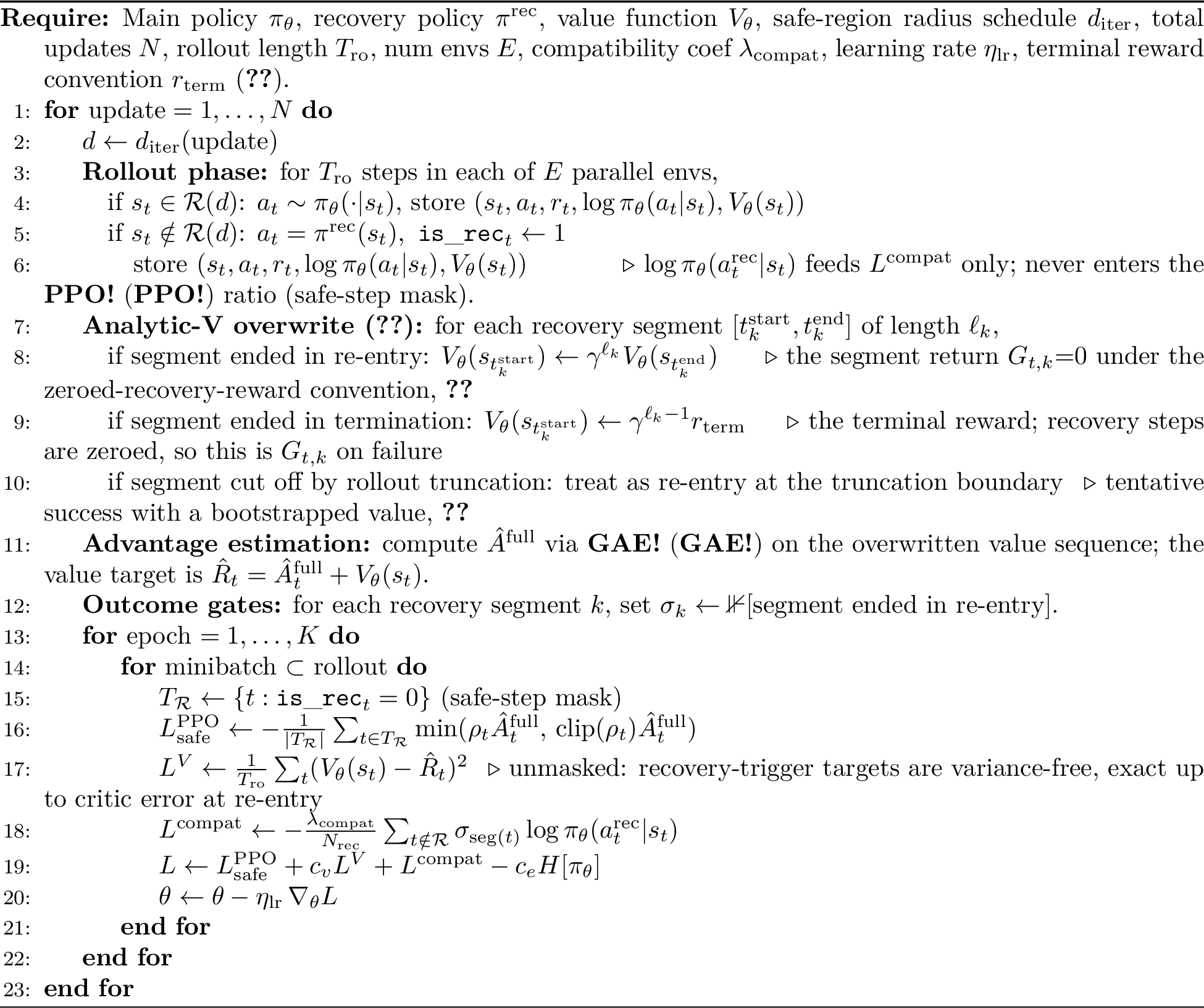
SafeExplorer assembles the three algorithmic pieces developed in the previous sections, the masked policy gradient (1, 2), the analytic recovery value (3), and the hard outcome-gated compatibility regularizer (4.4), into a single PPO update (2); the fourth piece, the objective-gap bound (2), needs no implementation beyond the curriculum below. Because each piece intervenes only where the recovery policy acts, the resulting algorithm is a small edit to a standard PPO implementation: the changes touch only the rollout’s recovery branch and the loss, everything else is unchanged. That locality keeps the method cheap: the added cost is one recovery-policy forward pass per triggered step plus segment bookkeeping (runtimes in 13).
This leaves one moving part, the safe-region radius that decides when recovery is triggered, which we anneal over training with a linear curriculum [58], [59]: \(d_{\mathrm{iter}}(u) = d_0 + \frac{u-1}{N}\,d_{\max}\), growing the region from a tight \(d_0\) to the per-environment \(d_{\max}\) over the \(N\) updates (\(d_0\), \(d_{\max}\), \(N\) in 13). 15.7 ablates logarithmic, step, and constant schedules on Ant, our least reliable recovery policy, where the linear schedule attains the highest reward. This annealing is the practical mechanism by which the recovery rate \(\alpha(\theta, d)\) falls over training (15.12), an empirical diagnostic for the gap-tightening predicted by 2.
6 Experimental Setup↩︎
Our experiments evaluate three claims. The first is the safety-reward trade-off of SafeExplorer against standard PPO, recovery-using baselines, and CMDP baselines, judged on both falls and reward. The second is the unreliable-recovery regime that most motivates the method, where the recovery policy itself often fails and the trade-off is hardest to win. The third asks which ingredient drives the gains: the unbiased masked gradient (1), the analytic recovery value (3), or the outcome-gated regularizer (1). A single metric adjudicates all three: the number of training falls a method incurs before first reaching task success, where success is \(80\%\) of the best final reward attained by any method in that environment. On Ant and Go1 that best method is SafeExplorer, so the reward winner partly sets its own bar; 1 therefore reports the underlying rewards and fall counts separately.
Environments. We evaluate on three continuous-control locomotion environments: HalfCheetah and Ant(custom MuJoCo [60]/Gymnasium [61] variants with a configurable safe-region
indicator; full specification in 14), and Go1, a Unitree Go1 quadruped built on the mujoco_menagerie model [62] with a velocity-tracking reward adapted from legged_gym [2]. The mechanism is identical across all three: the distance \(\mathcal{D}\) defining \(\mathcal{R}(d)\) is a \((z,
\mathrm{tilt})\) task-space distance to the nominal upright pose (exact formulas in 14.2), and each environment keeps its standard locomotion reward, zeroed only during recovery (4.3). The environments differ in how hard they make safety: HalfCheetah(planar, strong recovery) sets the baseline, Ant(3D, weaker recovery) tests whether the
compatibility regularizer compensates for an unreliable fall-back, and Go1(12-DoF quadruped) scales the claim to a higher-dimensional, multi-contact
platform.
Recovery policies. Each environment uses a separately pre-trained SAC [7] actor as \(\pi^{\mathrm{rec}}\): a stand-and-stabilize objective on its own environment, task terms disabled, no demonstrations, aggressively randomized resets (recipes in 14.3). At rollout time it takes the SAC mean action, deterministic, so it exercises the no-density case the masked gradient is built for (1). The Ant recovery policy is meaningfully weaker than the others, the most informative axis of variation: its strong control-magnitude penalty caps how aggressively it can correct, and the harder 3D stabilization needs those corrections (14).
The remaining choice is the radius \(d_{\max}\), the one quantity a skeptic might suspect was tuned. Unbiasedness holds for any \(d_{\max}\) (1), so no radius can manufacture statistical validity, though it still shapes results through the gap bound (2) and the curriculum. We set each \(d_{\max}\) (13) by a qualitative criterion, that the curriculum lowers the observable intervention rate (15.12), without a quantitative search. The fixed-\(d\) sweep (10) shows sensitivity to a constant radius that the curriculum mostly recovers (15.7); no systematic sweep varies \(d_{\max}\) under the curriculum, a limitation (15).
Variants compared. SafeExplorer (2) is compared against three external baselines spanning the established alternatives identified in 2. Standard PPO is the no-recovery extreme. Recovery RL [11] and Safe Legged [12] are on-policy ports of the two published recovery-using alternatives: both run inside the same PPO loop, sharing SafeExplorer’s safe-region trigger and frozen SAC recovery policy, and each isolates its published method’s data-handling rule at recovery steps, action relabeling for Recovery RL versus relabeling plus a fixed reward penalty of \(1\) for Safe Legged (exact rules and deviations in 12.7). A controlled ablation isolating each ingredient of SafeExplorer is reported in 8; additional soft-gate variants are in 15.4.
CMDP baselines. To position SafeExplorer against the standard no-recovery alternative, we compare to two CMDP solvers, CPO [39] and PPO-Lagrangian [14], [63], which act with a single policy and encode safety as a constraint on an indicator cost (1 per fall). We run both via OmniSafe [64] at settings matched to SafeExplorer, except the solvers’ default observation and reward normalization, which SafeExplorer does not use, favoring the baselines (15.14). 7.3 analyzes their constraint feasibility.
Training and evaluation. We train each variant for \(8\)M environment steps on HalfCheetah and Ant and \(16\)M on Go1(its higher-dimensional action space needs a longer horizon), with five random seeds. Final reward is the per-episode mean of the last \(10\%\) of training, computed from the unmodified task reward, not the recovery-zeroed learning signal; falls are the cumulative count over the full training run, a fall being a per-environment unhealthy termination (6), never a time-limit truncation. Tables report mean \(\pm\) standard deviation over seeds; the headline and ablation plots aggregate with interquartile means and \(95\%\) stratified-bootstrap confidence intervals [65]. A method’s falls-to-success is the cumulative falls before its trailing-mean reward first crosses the success bar; a method that never crosses it is counted as not reaching success, and falls-to-success aggregates use the succeeding seeds only (the \(k/n\) labels in 1). Shared PPO hyperparameters follow CleanRL’s defaults [66] and are listed in 4.
7 Main Results↩︎
7.1 SafeExplorer reaches task success with the fewest falls↩︎
Addressing our first claim, we compare all methods on the three environments: 1 reports falls-to-success with the per-method solve counts \(k/n\), 1 the separate final-reward and total-training-fall figures (different quantities, since total falls span the whole run, not just the climb to success), and 3 the per-metric rliable interquartile-mean view. SafeExplorer reaches success with the fewest training falls in every environment, an interquartile mean of \(12\) falls on HalfCheetah, \(17\) on Ant, and \(118\) on Go1. The advantage is most stark on Ant, where it is the only method to reach success at all, on all five seeds, while every baseline fails to cross the bar on any seed (quantified in 7.2). The separation also widens with the difficulty of staying safe: on Go1 the next-cheapest method after SafeExplorer to reach success at all is Recovery RL on a single seed (\(309\) falls), with PPO-Lagrangian and PPO at \(9{,}658\) and \(15{,}320\). The same lead shows up in the table’s lifetime view: measured as total training falls (1), SafeExplorer reduces falls over PPO by \(\mathbf{233\times}\) on HalfCheetah, \(\mathbf{48\times}\) on Ant, and \(\mathbf{26\times}\) on Go1 while matching or beating PPO’s final reward.
| 2-3(lr)4-5(lr)6-7 Method | Reward \(\uparrow\) | Falls \(\downarrow\) | Reward \(\uparrow\) | Falls \(\downarrow\) | Reward \(\uparrow\) | Falls \(\downarrow\) |
| PPO (no recovery) | \(3246\pm521\) | \(3311\pm940\) | \(308\pm165\) | \(36467\pm14598\) | \(3347\pm215\) | \(18683\pm1403\) |
| Recovery RL | \(1951\pm1423\) | \(947\pm1831\) | \(76\pm25\) | \(53535\pm7611\) | \(3136\pm511\) | \(1689\pm1379\) |
| Safe Legged | \(\mathbf{4054\pm604}\) | \(1552\pm1084\) | \(83\pm20\) | \(53548\pm11682\) | \(2347\pm353\) | \(3022\pm1225\) |
| CPO | \(2835\pm403\) | \(23\pm30\) | \(1047\pm106\) | \(899\pm117\) | \(359\pm48\) | \(39613\pm2498\) |
| PPO-Lagrangian | \(2939\pm414\) | \(18\pm19\) | \(1339\pm402\) | \(5094\pm2774\) | \(3915\pm953\) | \(12572\pm1636\) |
| (ours) | \(3581\pm971\) | \(\mathbf{14\pm8}\) | \(\mathbf{2857\pm129}\) | \(\mathbf{754\pm463}\) | \(\mathbf{5594\pm177}\) | \(\mathbf{731\pm177}\) |
4pt
![Figure 1: Training falls to reach task success (success =80\% of the best final reward in each environment), interquartile mean with 95\% bootstrap confidence intervals [65]; log axis, fewer falls is better. Labels show the seeds reaching success (k/n); never-reachers are marked at right. Baselines are gray, SafeExplorer ablation variants (8) blue, and SafeExplorer the red star, which reaches success with the fewest falls in every environment and is the only method to reach it on Ant.](/article/2607.08925/figures/falls_to_success_80pct.png "fig:")
Reading the environments one at a time, the same ranking holds but the reason shifts with how hard safety is. On HalfCheetah, where the recovery policy is reliable, PPO is competitive on reward but pays for it in falls, while SafeExplorer matches that reward at a fraction of the falls. On Go1, the larger action space and longer horizon make PPO highly unsafe, while Recovery RL and Safe Legged control falls only at substantial reward cost and SafeExplorer attains both the highest reward and the lowest fall count. Ant is the informative exception: the ranking still favors SafeExplorer, but it behaves differently because the recovery policy itself is unreliable, the case we isolate next in 7.2.
This dependence on recovery is exactly what 2 predicts: 15.12 confirms on body-matched 5-seed runs that the gap \(J^{\mathrm{mix}}(\theta_k) - J(\theta_k)\) tracks the recovery rate \(\alpha(\theta, d)\), closing to seed noise on HalfCheetah and Ant, where the policy becomes self-stable, and settling at a proportional residual on Go1, where it does not.
Per-environment learning curves are deferred to 4 in 15.
7.2 The unreliable-recovery regime: Ant↩︎
This subsection addresses our second claim, the unreliable-recovery regime: 7.1 cannot show why SafeExplorer remains effective where the recovery policy itself fails, so we isolate the one environment where that happens, Ant, whose SAC recovery is markedly less reliable. Replaying the recovery from the states a trained policy actually drives it into, it completes the segment only \(70\) to \(91\%\) of the time on Ant, against \(97\) to \(100\%\) on HalfCheetah and Go1(one representative run per environment; 7). The recovery-based baselines reveal the latter: PPO, Recovery RL, and Safe Legged all fail catastrophically (\(36\)k to \(54\)k falls, reward \(\le 308\)). The mechanism is a feedback cycle, because when the recovery policy is unreliable, any method that relies on it reactively keeps re-entering unsafe states, recovery keeps failing, and the agent never learns to avoid them unaided. SafeExplorer breaks that cycle and alone reaches the \(2286\) success bar, at \(2857\) reward and \(754\) falls, an order of magnitude fewer falls than any other recovery-using method; the strongest baselines, PPO-Lagrangian and CPO, reach \(1339\) and \(1047\). The ablations pinpoint why: every variant that drops the hard outcome gate, including the soft-gate variants, also fails on Ant(8); the gate, not the masked gradient or the analytic value, supplies the fallback skill when recovery is unreliable.
7.3 Comparison to CMDP baselines↩︎
This subsection completes our first claim by comparing SafeExplorer against the CMDP alternative to a recovery policy, which casts safety as a constraint and solves the resulting CMDP rather than intervening on the trajectory. CPO and PPO-Lagrangian, the trust-region and Lagrangian solvers, appear in 1 and 1 with a cost of \(1\) per fall, at settings identical to SafeExplorer. SafeExplorer attains the highest reward of the three in every environment and the fewest total training falls on Ant and Go1, with all three methods low and within seed noise on HalfCheetah(1). The more revealing comparison is constraint feasibility: whether each solver keeps the falls it promised to.
The constrained solvers’ poor safety on the hard environments is not under-tuning. Each CMDP solver is configured with a cost limit on falls, as its formulation requires, and meets it on HalfCheetah where staying safe is easy, but violates its own limit on Ant and Go1 by up to \(19\times\): CPO converges to an episodic cost of \(0.96\) on Go1 against the \(0.05\) budget it was set, and even incurs more Go1 falls than unconstrained PPO at a tenth of the reward (15.14). Constraint satisfaction thus holds where safety is easy and fails exactly where the safe-region intervention is needed. The difference is one of mechanism: the CMDP baselines act alone and only penalize the violation after the fact, whereas SafeExplorer acts on the safe region directly, which is why it keeps falls low where the constrained solvers cannot.
8 Ablation Analysis↩︎
This section addresses our third claim, which ingredient drives SafeExplorer’s gains over prior recovery-using methods. We isolate each of its three new ingredients with a ladder of controlled variants that share the recovery policy and curriculum and differ only at recovery steps. The ladder starts from the biased update those methods use, which keeps recovery transitions as if the main policy had generated them (a learned-critic on-policy gradient), and turns on one ingredient at a time: Unmasked PG is that biased baseline; masked, learned \(V\) switches to the unbiased masked policy gradient (1); masked, analytic \(V\) adds the analytic recovery value (3); and SafeExplorer adds the hard outcome gate (6 ), with PPO (no recovery) anchoring the no-intervention end. 1 ranks these variants by falls-to-success and 5 (15.3) gives the complementary reward-vs-falls view. Each ingredient contributes a distinct improvement, attributed rung by rung below.
The first rung, the masked policy gradient (1), is the foundation. Its biased alternative, Unmasked PG, reaches competitive or higher reward on HalfCheetah and Go1, but pays \(14\times\), \(7\times\), and \(4\times\) more falls than SafeExplorer on HalfCheetah, Ant, and Go1(8), and is ill-posed for deterministic recovery. Masking removes that bias, the prerequisite for the next two ingredients.
Removing the bias exposes a second problem: the unbiased gradient is sparse at the safe-region boundary, so the masked, learned-\(V\) variant alone regresses to \(1982\) reward on HalfCheetah, the lowest of any rung (8). The analytic recovery value (3) supplies dense, correct targets exactly there, lifting HalfCheetah reward to \(3870\), the largest single-ingredient gain on that environment (\(+1888\)).
The top rung adds the hard outcome gate (SafeExplorer), which dominates on safety in every environment and supplies the largest single-ingredient reward gains on Go1 and Ant(\(+1121\) and \(+2683\); 8), where the analytic value alone leaves reward flat; it is the only variant to reach the Ant success bar (\(2286\); next best \(1253\)), the strongest evidence for the imitation reading of \(C_\theta(\tau)\) (4.4).
In the \(\lambda_{\mathrm{compat}}\) sweep (9; HalfCheetah and Ant only, the default transferred to Go1 untested), HalfCheetah reward stays at \(4768\) to \(5783\) across \([10^{-3}, 1]\), peaking at \(10^{-2}\), but falls are minimized at the \(10^{-3}\) default (\(47\)) and rise \(8\times\) within a decade (\(374\) at \(10^{-2}\)); we choose the default on falls, not reward. 15 reports the rest: robustness to hyperparameters and noise ([app:lambda-sensitivity,app:fixed-d,app:curr-shape,app:compat-norm,app:action-noise]), the soft-gate variants (15.4), compute-scaling (15.8), the full ladder (15.3), and a failure-mode catalog (15.11).
9 Discussion and Limitations↩︎
When the method helps, and when it does not. SafeExplorer’s advantage is smallest when PPO is already safe and recovery is reliable, and largest in the opposite regimes: weak recovery (Ant), dangerous unaided PPO (Go1). The hard outcome gate makes this work: a soft gate imitates failed recovery actions and degrades both metrics (15.4). We treat the recovery policy as a permanent fallback, not temporary scaffolding: on Go1 it stays mildly engaged (\(\alpha(\theta, d)\approx 0.05\)) even at \(16\)M steps, and keeping it available is what bounds falls there (15.12); our claim is reduced training falls, not their elimination.
Assumptions behind the guarantees. The analytic value (3) is exact only under deterministic dynamics and recovery. Under noise it becomes a single-sample estimate, unbiased up to critic error at re-entry, favorable in practice since \(\pi^{\mathrm{rec}}\) is near-deterministic; a multi-sample extension is in 11.5. The objective-gap bound (2) is controlled by the unobservable out-of-region rate \(\beta(\theta, d)\), tracked via the observable \(\alpha(\theta, d)\) as a diagnostic (15.12). A certified observable bound remains open (a deterministic recovery makes the natural simulation-lemma bound vacuous; routes in 11.7).
Generality of the compatibility regularizer. The gate is also what makes the regularizer general: without it \(L^{\mathrm{compat}}\) is DAgger-style imitation (4), so outcome-gated imitation should transfer to other teacher-intervention settings, human-in-the-loop RL [35] or JSRL [17].
Beyond locomotion. That transfer argument is theoretical; our evaluation is locomotion-only, though the correction applies wherever a fixed recovery policy takes over at unsafe states (a scripted reset in manipulation, an emergency-stop in driving); validating these is future work. The method also presupposes a pre-trained recovery policy and a hand-designed distance \(\mathcal{D}\), whose acquisition cost is excluded from the reported budgets ([app:hyperparams,app:env]).
10 Conclusion↩︎
We built SafeExplorer, an on-policy RL algorithm for safety-critical control that, as a single PPO update, reduces training-time falls by \(26\times\) to \(233\times\) across three locomotion environments while matching or beating standard PPO on reward.
These gains rest on a theoretical foundation for RL with an external recovery policy: a masked policy-gradient theorem unbiased for the mixed-policy return under any recovery, an objective-gap bound with an exact fixed point, an analytic recovery value, and an outcome-gated compatibility regularizer, all instantiated for safe-region intervention to minimize training falls.
11 Full Proofs↩︎
11.1 Proof of 1 (unbiased gradient of \(J^{\mathrm{mix}}(\theta)\))↩︎
Proof. Starting from the definition, \(J^{\mathrm{mix}}(\theta) = \int p_\theta^{\mathrm{mix}}\, r(\tau)\, d\tau.\) Under 1, differentiation and integration commute: \(\nabla_\theta J^{\mathrm{mix}}(\theta) = \int \nabla_\theta p_\theta^{\mathrm{mix}}\, r(\tau)\, d\tau.\) Factor \(p_\theta^{\mathrm{mix}}\) explicitly by partition membership of the visited states: \[\label{eq:thm1-factored} p_\theta^{\mathrm{mix}} = \underbrace{p(s_1)}_{\text{no }\theta} \cdot \underbrace{\prod_{t : s_t \in \mathcal{M}} \pi_\theta(a_t \mid s_t)}_{\text{only \theta-dependent factor}} \cdot \underbrace{\prod_{t : s_t \notin \mathcal{M}} \mu(a_t \mid s_t)}_{\text{no }\theta} \cdot \underbrace{\prod_{t=1}^T P(s_{t+1} \mid s_t, a_t)}_{\text{no }\theta},\tag{8}\] where \(\mu(\cdot|s)\) denotes the (possibly Dirac) \(\theta\)-independent action measure at \(s \notin \mathcal{M}\). Equation 8 is an equality of measures on trajectory space and does not require \(\mu\) to have a Lebesgue density. Deterministic, stochastic, point-mass at a hand-coded action, and pre-trained-policy measures are all covered. Only the \(\mathcal{M}\)-step factor depends on \(\theta\). By the product rule and the score-function identity applied factor-wise, \[\nabla_\theta p_\theta^{\mathrm{mix}} = p_\theta^{\mathrm{mix}}\, \sum_{t : s_t \in \mathcal{M}} \nabla_\theta \log \pi_\theta(a_t \mid s_t).\] No gradient of \(\mu\) appears, because \(\mu\) carries no \(\theta\)-dependence; at no point do we evaluate \(\log\) of a Dirac measure. Substituting back, \[\nabla_\theta J^{\mathrm{mix}}(\theta) = \mathbb{E}_{\tau \sim p_\theta^{\mathrm{mix}}}\!\left[ \Big(\sum_{t : s_t \in \mathcal{M}} \nabla_\theta \log \pi_\theta(a_t\mid s_t)\Big)\, r(\tau) \right]. \qedhere\] ◻
Corollaries ([cor:safe-region-gradient,cor:jsrl-gradient,cor:shielded-gradient]). The proof never used the specific form of \(\mu\), only that \(\mu\) carries no \(\theta\)-dependence, so each corollary follows by simply instantiating the pair \((\mathcal{M}, \mu)\). The safe-region intervention case (\(\mathcal{M} = \mathcal{R}\), \(\mu = \pi^{\mathrm{rec}}\)) is the body of this paper. The Jump-Start RL case (\(\mathcal{M} = \{(s,t) : t \ge h\}\) for a per-trajectory handoff step \(h\), \(\mu = \pi^{\mathrm{teach}}\) for a fixed teacher) inherits the same factorization: the teacher is \(\theta\)-independent, the handoff step is data-dependent but not \(\theta\)-dependent, and the score function evaluates only on the student-controlled tail of each trajectory. The state-triggered shielded RL case (\(\mathcal{M} = \{s : \Sigma \text{ does not engage at } s\}\), \(\mu(a\mid s) = \delta(a - \sigma(s))\) for the shield’s corrective action \(\sigma\)) inherits the same factorization with \(\mu\) a Dirac measure that the proof’s factor-level differentiation handles directly. The common payoff is the same in all three: the IS fix is ill-defined when \(\mu\) has no density at the relevant states, whereas the factor-level proof never forms the ratio and so bypasses the need for a density on \(\mu\). We state the two non-safe-region specializations formally for reference.
Corollary 4 (Jump-Start RL [17]). Let \(\pi^{\mathrm{teach}}\) be a fixed teacher policy and \(h\) a per-trajectory handoff step. Take \(\mathcal{M} = \{(s, t) : t \ge h\}\) (states reached after handoff; the timestep \(t\) is absorbed into the state, standard for finite-horizon MDPs, so \(\mathcal{M}\) is a subset of the augmented state space) and \(\mu = \pi^{\mathrm{teach}}\). Then 1 gives an unbiased gradient of the student’s contribution to the mixed return, where the score function is evaluated only on the student-controlled tail of each trajectory.
Corollary 5 (State-triggered shielded RL). Let \(\Sigma\) be a state-triggered shield, whose engagement is decided by the state alone and which, at unsafe states, replaces the proposed action with a \(\theta\)-independent corrective action \(\sigma(s)\). Take \(\mathcal{M} = \{s : \Sigma\text{ does not engage at }s\}\) and \(\mu(a\mid s) = \delta(a - \sigma(s))\). Then 1 gives an unbiased gradient evaluated only at unshielded states, with no density required on the shield’s correction.
Action-triggered shields, as in [42], decide the override from the proposed action \(a \sim \pi_\theta(\cdot \mid s)\): at states where only some actions are unsafe, the executed-action distribution mixes \(\pi_\theta\) restricted to safe actions with the correction weighted by the \(\theta\)-dependent probability of proposing an unsafe action, so it depends on \(\theta\) and falls outside 1’s hypothesis of a \(\theta\)-independent \(\mu\).
Truncated importance sampling. One might hope that the singularity is only a problem for the naive IS estimator and that a more careful clipped estimator escapes it. It does not. Truncated-IS estimators such as V-trace [31] and Retrace [32] reach the mixed-policy gradient by clipping the importance ratio \(p_\theta/p_\theta^{\mathrm{mix}}\), but that ratio is still undefined at the deterministic-recovery steps where \(\mu\) is a point mass. Clipping bounds variance downstream of the singularity rather than removing it. The factor-level proof above avoids the ratio entirely, which is exactly why it extends to the deterministic recovery policy our method uses.
11.2 Proof of 2 (objective-gap bound)↩︎
This subsection and the remainder of the appendix work in the infinite-horizon discounted convention fixed in 3, under which \(V^{\pi^{\mathrm{mix}}_\theta}\), \(Q^{\pi^{\mathrm{mix}}_\theta}\), \(A^{\pi^{\mathrm{mix}}_\theta}\), and the normalized discounted visitations \(\nu^{\pi_\theta}\), \(\nu^{\pi^{\mathrm{mix}}_\theta}\) are stationary.
Proof. 1 shows we optimize \(J^{\mathrm{mix}}\) rather than the deployment objective \(J\), so the question is how far apart the two can be. We bound the gap by routing it through the states where the two policies actually differ. By the Performance Difference Lemma [55], \[\label{eq:pdl} J(\theta) - J^{\mathrm{mix}}(\theta) = \frac{1}{1-\gamma}\, \mathbb{E}_{s \sim \nu^{\pi_\theta},\, a \sim \pi_\theta(\cdot|s)}\!\left[ A^{\pi^{\mathrm{mix}}_\theta}(s, a) \right],\tag{9}\] where \(A^{\pi^{\mathrm{mix}}_\theta}(s,a) = Q^{\pi^{\mathrm{mix}}_\theta}(s,a) - V^{\pi^{\mathrm{mix}}_\theta}(s)\). Split the expectation by the safe region: \[J(\theta) - J^{\mathrm{mix}}(\theta) = \frac{1}{1-\gamma}\!\left( \underbrace{\mathbb{E}_{s \in \mathcal{R}}[\cdot]}_{=\,0} + \mathbb{E}_{s \notin \mathcal{R}}[\cdot] \right).\] On \(s \in \mathcal{R}\), both \(\pi_\theta\) and \(\pi^{\mathrm{mix}}_\theta\) sample from \(\pi_\theta\), so the inner expectation \(\mathbb{E}_{a \sim \pi_\theta(\cdot|s)}[A^{\pi^{\mathrm{mix}}_\theta}(s,a)] = 0\) by definition of \(V^{\pi^{\mathrm{mix}}_\theta}\). On \(s \notin \mathcal{R}\), \(|A^{\pi^{\mathrm{mix}}_\theta}(s,a)| \le |Q^{\pi^{\mathrm{mix}}_\theta}(s,a)| + |V^{\pi^{\mathrm{mix}}_\theta}(s)| \le 2r_{\max}/(1-\gamma)\) since both \(|Q|\) and \(|V|\) are bounded by \(r_{\max}/(1-\gamma)\). Therefore \[|J(\theta) - J^{\mathrm{mix}}(\theta)| \le \frac{1}{1-\gamma} \cdot \frac{2r_{\max}}{1-\gamma} \cdot \Pr_{s \sim \nu^{\pi_\theta}}[s \notin \mathcal{R}] = \frac{2r_{\max}}{(1-\gamma)^2}\, \beta(\theta, d). \qedhere\] ◻
Bound on the out-of-region rate \(\beta(\theta, d)\) (4.2). The gap above scales with \(\beta(\theta, d)\), so the bound is only useful once \(\beta(\theta, d)\) itself is controlled. 4.2 uses \(\beta(\theta, d)\le \eta\gamma/(1-\gamma) \le \eta/(1-\gamma)\), which we now derive from the per-step invariance slack, under the additional hypothesis that episodes start inside the safe region, \(\operatorname{supp}\, p(s_1) \subseteq \mathcal{R}(d)\) (otherwise the initial step alone contributes \((1-\gamma)\Pr[s_1 \notin \mathcal{R}]\) to \(\beta(\theta, d)\) even with \(\eta = 0\)). All three of our environments satisfy the hypothesis: episodes reset to an upright pose inside the region. Starting from a reachable initial state \(s_0 \in \mathcal{R}\) (this derivation counts steps from zero, so \(s_0\) here is the \(s_1\) of the trajectory notation), 2 gives \(\Pr[s_0, \dots, s_t \in \mathcal{R}] \ge (1-\eta)^t\). Since \(\{s_t \in \mathcal{R}\} \supseteq \{s_0, \dots, s_t \in \mathcal{R}\}\), the marginal in-region probability dominates the all-stay probability, \(\Pr[s_t \in \mathcal{R}] \ge (1-\eta)^t\), hence \(\Pr[s_t \notin \mathcal{R}] \le 1 - (1-\eta)^t\). With the discounted state-visitation \(\beta(\theta, d)= (1-\gamma)\sum_{t\ge 0} \gamma^t \Pr[s_t \notin \mathcal{R}]\), \[\beta(\theta, d)\le (1-\gamma)\sum_{t\ge 0} \gamma^t \big(1 - (1-\eta)^t\big) = \frac{\eta\gamma}{1 - \gamma(1-\eta)} \le \frac{\eta\gamma}{1-\gamma} \le \frac{\eta}{1-\gamma},\] the last step using \(1-\gamma(1-\eta) \ge 1-\gamma\) and \(\gamma \le 1\).
Train-to-deploy reward gap (footnote in 4.3). The training-signal convention of 3 (zero per-step reward during recovery, one-time terminal reward \(r_{\mathrm{term}}\)) and the unmodified task reward differ only at states outside \(\mathcal{R}\) (and through the one-time \(r_{\mathrm{term}}\)). Bounding the per-step discrepancy by \(r_{\max}+ |r_{\mathrm{term}}|\) on those steps and summing the discounted visitation under \(\pi_\theta\), the returns the two conventions induce under \(\pi_\theta\) differ by at most \((r_{\max}+ |r_{\mathrm{term}}|)\,\beta(\theta, d)/(1-\gamma)\), so the train-to-deploy chain is controlled by the same \(\beta(\theta, d)\) as 2.
11.3 Proof of 3 (conditional fixed point)↩︎
Proof. The gap bound of 2 leaves \(\beta(\theta, d)\) free, so the natural endpoint of the analysis is the case that drives \(\beta(\theta, d)\) to zero. The corollary splits into two readings of when that happens.
Reading (R-A): If \(\mathcal{R}(d_{\max})\) covers the reachable state space, then \(\Pr[s \notin \mathcal{R}(d_{\max})] = 0\) under any action distribution, including \(\pi_\theta\) alone. Hence \(\beta(\theta, d_{\max}) = 0\), and 4 gives \(J^{\mathrm{mix}}(\theta) = J(\theta)\) exactly. Furthermore, \(\pi^{\mathrm{mix}}_\theta\) is identical to \(\pi_\theta\) on the reachable support of \(p_\theta(\tau)\) (recovery is never engaged).
Reading (R-B): If \(\mathcal{R}(d_{\max})\) is strictly contained in the reachable state space, the theory no longer forces \(\pi_\theta\) to remain in \(\mathcal{R}\), so its invariance slack \(\eta_\star := \eta(\theta,d_{\max}) \ge 0\) (2) need not be zero. Substituting \(\beta \le \eta_\star/(1-\gamma)\) (derived above under the initial-state hypothesis \(\operatorname{supp}\, p(s_1) \subseteq \mathcal{R}\)) into 4 gives the upper bound \(|J(\theta)-J^{\mathrm{mix}}(\theta)| \le 2r_{\max}\eta_\star / (1-\gamma)^3\), which, unlike (R-A), is not pinned to zero. Whether \(\eta_\star\) (and hence the gap) is small is environment-dependent: 15.12 finds \(\eta_\star \to 0\) on HalfCheetah and Ant, where the gap closes to seed noise, and \(\eta_\star > 0\) on Go1, where a proportional residual remains. ◻
11.4 Proof of 3 (analytic recovery value)↩︎
Proof. The gradient and gap results above treat \(V^{\pi^{\mathrm{mix}}_\theta}\) as given; what remains is to compute it cheaply on the recovery segments themselves, where the trajectory is no longer under the agent’s control. By the definition of \(V^{\pi^{\mathrm{mix}}_\theta}\), \(V^{\pi^{\mathrm{mix}}_\theta}(s_t) = \mathbb{E}_{\tau \sim p^{\mathrm{mix}}_\theta(\tau)| s_t}\!\left[ \sum_{j=0}^{\infty} \gamma^j r_{t+j} \right].\) Under deterministic dynamics and deterministic recovery, the trajectory starting from a recovery-triggering state \(s_t\) is fully determined for the duration of the recovery segment \([t, t+k]\). The expectation collapses. Two cases:
- Recovery success
-
(\(s_{t+k} \in \mathcal{R}\)): the realized return over the segment is \(G_{t,k} = \sum_{j=0}^{k-1}\gamma^j r_{t+j}\). From \(s_{t+k}\) the agent resumes under \(\pi^{\mathrm{mix}}_\theta\) with value \(V^{\pi^{\mathrm{mix}}_\theta}(s_{t+k})\). Hence \(V^{\pi^{\mathrm{mix}}_\theta}(s_t) = G_{t,k} + \gamma^k V^{\pi^{\mathrm{mix}}_\theta}(s_{t+k})\).
- Recovery failure
-
(terminal): the realized return is \(G_{t,k}\) over the \(k\) deterministic steps, the episode ends, no further reward accrues. Hence \(V^{\pi^{\mathrm{mix}}_\theta}(s_t) = G_{t,k}\).
Combining gives ?? . Our implementation instantiates this general statement under a chosen reward: zero per-step reward during recovery and a one-time terminal reward \(r_{\mathrm{term}}\) accrued at the final segment step (\(t{+}k{-}1\)) on failure. The terminal penalty is thus the only nonzero contribution to the segment return \(G_{t,k} = \sum_{j=0}^{k-1}\gamma^j r_{t+j}\), which is therefore \(0\) on success and \(\gamma^{k-1} r_{\mathrm{term}}\) on failure, matching ?? . ◻
11.5 Analytic value under stochastic dynamics↩︎
The closed form just derived rests on the determinism assumption, so it is worth asking what survives when that assumption is relaxed. 3 assumes deterministic \(P\) and \(\pi^{\mathrm{rec}}\). Under process noise or stochastic recovery, the realized \(\gamma^k V_\theta(s_{t+k})\) is no longer equal to \(V^{\pi^{\mathrm{mix}}_\theta}(s_t)\). It becomes a single Monte-Carlo realization drawn from the distribution over post-trigger trajectories, whose variance grows with the noise of \(P\) and \(\pi^{\mathrm{rec}}\) accumulated over the segment. Two natural extensions preserve the spirit of bypassing critic bootstrapping across recovery. (i) A multi-sample MC target: re-roll the recovery \(M\) times from \(s_t\) (where the simulator supports state-resets) and average \(G_{t,k_m} + \gamma^{k_m} V_\theta(s_{t+k_m})\) across the \(M\) realizations. This is an unbiased estimator of \(V^{\pi^{\mathrm{mix}}_\theta}(s_t)\) whose variance falls as \(1/M\). (ii) The single-sample plug-in we already use is an unbiased one-sample MC estimate of \(V^{\pi^{\mathrm{mix}}_\theta}(s_t)\). Its bias is zero in expectation, but its single-realization noise reaches downstream GAE. The bias-variance trade-off is favorable in our setting because \(\pi^{\mathrm{rec}}\) is approximately deterministic in practice (MPC, greedy SAC), so the per-segment variance is small. A formal analysis under controlled stochasticity, and the regime where (i) is worth the extra simulator calls, is left to follow-up.
11.6 Proof of 4↩︎
The recovery segments that supplied the analytic value also supply state-action pairs for the compatibility regularizer, and identifying its limiting cases shows that this loss is not an ad-hoc addition but a familiar imitation objective in disguise.
Proposition 4 (Special cases of the compatibility regularizer). Let \(\pi^{\mathrm{rec}}\) be deterministic, so \(a_t^{\mathrm{rec}} = \pi^{\mathrm{rec}}(s_t)\) at recovery-controlled states, and consider the gate-set choice \(\sigma_k \equiv 1\) for all segments.
Behavioral cloning on the recovery dataset. Under \(\sigma_k \equiv 1\), \[\label{eq:compat-bc-limit} L^{\mathrm{compat}}_{\sigma \equiv 1}(\theta) = -\frac{\lambda_{\mathrm{compat}}}{N_{\mathrm{rec}}} \sum_{t : s_t \notin \mathcal{R}} \log \pi_\theta\!\left(\pi^{\mathrm{rec}}(s_t) \mid s_t\right),\qquad{(2)}\] the (scaled) negative log-likelihood of \(\pi_\theta\) on the dataset \(\mathcal{B} = \{(s_t, \pi^{\mathrm{rec}}(s_t)) : s_t \notin \mathcal{R}\}\) of recovery-controlled state-action pairs collected from rollouts of \(\pi^{\mathrm{mix}}_\theta\). Equivalently, \(L^{\mathrm{compat}}_{\sigma \equiv 1}\) is the per-step behavioral-cloning objective applied to \(\pi^{\mathrm{rec}}\)’s actions at the states \(\pi^{\mathrm{mix}}_\theta\) visits during recovery.
A region-restricted DAgger aggregation step. The dataset \(\mathcal{B}\) is collected as in one iteration of DAgger [18] with the teacher queried only on the intervention set: states are visited under the mixed roll-out policy \(\pi^{\mathrm{mix}}_\theta\) (predominantly student-induced up to the safe-region boundary), and labels are the controller \(\pi^{\mathrm{rec}}\)’s actions at the recovery-controlled states only, whereas DAgger labels every visited state. Minimizing \(L^{\mathrm{compat}}_{\sigma \equiv 1}\) as the per-iteration training step then reproduces a region-restricted analogue of DAgger’s update with \(\pi^{\mathrm{rec}}\) in the teacher role and \(\pi_\theta\) as the student.
Outcome gate as a designer filter. The general gate \(\sigma_k \in \{0, 1\}\) restricts \(\mathcal{B}\) to recovery segments that re-entered \(\mathcal{R}\), discarding the rest. JSRL-style mixed-policy data collection [17] produces the same mixed-policy roll-out distribution but does not include an imitation loss. \(L^{\mathrm{compat}}\) with \(\sigma_k \equiv 1\) supplies the analogous student-imitation step that the JSRL algorithm itself omits. What is new in the case \(\sigma_k \not\equiv 1\) is gating imitation of an external recovery controller* by the realized success of its multi-step segment, as opposed to gating by value estimates of one’s own past actions [56] or of demonstrations [57].*
Proof. (a) From 7 with \(w_t = \sigma_{\operatorname{seg}(t)}\), where \(\operatorname{seg}(t)\) is the index of the recovery segment containing \(t\) (4.4), and the assumption \(\sigma_k \equiv 1\), \[L^{\mathrm{compat}}_{\sigma \equiv 1}(\theta) = -\frac{\lambda_{\mathrm{compat}}}{N_{\mathrm{rec}}} \sum_{t : s_t \notin \mathcal{R}} 1 \cdot \log \pi_\theta(a^{\mathrm{rec}}_t \mid s_t) = -\frac{\lambda_{\mathrm{compat}}}{N_{\mathrm{rec}}} \sum_{t : s_t \notin \mathcal{R}} \log \pi_\theta\!\left(\pi^{\mathrm{rec}}(s_t) \mid s_t\right),\] using \(a_t^{\mathrm{rec}} = \pi^{\mathrm{rec}}(s_t)\) for deterministic \(\pi^{\mathrm{rec}}\). This is, up to the constant scale \(\lambda_{\mathrm{compat}}/ N_{\mathrm{rec}}\), the empirical negative log-likelihood of \(\pi_\theta\) on the dataset \(\mathcal{B} = \{(s_t, \pi^{\mathrm{rec}}(s_t)) : s_t \notin \mathcal{R}\}\), the (population-level) maximum-likelihood / behavioral-cloning objective for \(\pi_\theta\) on \(\mathcal{B}\).
(b) The dataset \(\mathcal{B}\) is collected by rolling out \(\pi^{\mathrm{mix}}_\theta\), retaining the state-action pairs at the unsafe-region timesteps. Under \(\pi^{\mathrm{mix}}_\theta\), \(\pi_\theta\) controls the rollout up to the first exit from \(\mathcal{R}\) (so the visited boundary state \(s_t\) has \(\pi_\theta\)-induced distribution), and \(\pi^{\mathrm{rec}}\) provides actions thereafter. This matches the data-collection rule of a single DAgger iteration with \(\pi^{\mathrm{rec}}\) as the teacher and \(\pi_\theta\) as the student, states visited under the mixed roll-out policy and labels from the teacher, except that the teacher is queried only at the recovery-controlled states rather than at every visited state as in [18]. Minimizing \(L^{\mathrm{compat}}_{\sigma \equiv 1}\) as the per-iteration update therefore reproduces a region-restricted analogue of the DAgger aggregation step.
(c) For general \(\sigma_k \in \{0, 1\}\), the regularizer is \[L^{\mathrm{compat}}(\theta) = -\frac{\lambda_{\mathrm{compat}}}{N_{\mathrm{rec}}} \sum_{k} \sigma_k \sum_{t : s_t \notin \mathcal{R},\, \operatorname{seg}(t) = k} \log \pi_\theta\!\left(\pi^{\mathrm{rec}}(s_t) \mid s_t\right),\] i.e.the behavioral-cloning objective restricted to the sub-dataset \(\mathcal{B}_{\mathrm{succ}} = \{(s_t, \pi^{\mathrm{rec}}(s_t)) : s_t \notin \mathcal{R},\, \sigma_{\operatorname{seg}(t)} = 1\}\) collected from segments that re-entered \(\mathcal{R}\). JSRL [17] likewise rolls out a mixed teacher-then-student policy but trains the student only by reinforcement on the student-controlled tail. It does not include a teacher-imitation step. The \(\sigma_k \equiv 1\) specialization of \(L^{\mathrm{compat}}\) is the analogous imitation loss JSRL omits. In the \(\sigma_k \not\equiv 1\) case, the new element is the gating criterion and target: imitation of an external recovery controller gated by the realized success of its multi-step segment, rather than by value estimates of the agent’s own past actions [56] or of demonstrations [57]. ◻
11.7 Sketch: why an observable upper bound on \(\beta\) is hard in continuous actions↩︎
The bound on \(\beta(\theta, d)\) above is stated in terms of the per-step invariance slack \(\eta\), which is not directly measurable; a bound in terms of an observable quantity would be far more useful, and we close by explaining why that is hard. A natural attempt is to bound \(\beta\) by the observable recovery rate \(\alpha\) via a simulation-lemma argument: \(\beta = \Pr_{\nu^{\pi_\theta}}[s\notin\mathcal{R}] \le \alpha + \mathrm{TV}(\nu^{\pi_\theta}, \nu^{\pi^{\mathrm{mix}}_\theta}).\) Here \(\mathrm{TV}(\cdot,\cdot)\) denotes total variation (TV) distance. The TV term can in turn be bounded by the expected per-step TV between \(\pi_\theta\) and \(\pi^{\mathrm{mix}}_\theta\) via the standard simulation lemma [67]. But on unsafe states \(\pi^{\mathrm{mix}}_\theta\) collapses to a Dirac (deterministic recovery) while \(\pi_\theta\) remains absolutely continuous. The per-step TV at unsafe states is \(1\) pointwise, so the simulation-lemma term contributes a full \(1/(1-\gamma) > 1\), and the bound \(\beta \le \alpha + 1/(1-\gamma)\) exceeds \(1\) and is therefore vacuous (since \(\beta \le 1\) trivially). Routes that may produce a non-vacuous bound include (i) replacing the deterministic recovery with a smoothed (LSE / Gaussian-mixture) variant whose TV with \(\pi_\theta\) is finite, (ii) Wasserstein-action-gap bounds under known dynamics Lipschitz constants, and (iii) periodic offline evaluation of \(\pi_\theta\) alone. We sketch (i) below and leave a complete treatment to follow-up work.
Sketch via smoothed recovery. Replace \(\pi^{\mathrm{rec}}(\cdot|s) = \delta(a - \bar a(s))\) with \(\tilde{\pi}_\mathrm{rec}(\cdot|s) = \mathcal{N}(\bar a(s), \sigma_\mathrm{rec}^2 I)\) for small \(\sigma_\mathrm{rec}\). Then both \(\pi_\theta(\cdot|s)\) and \(\tilde{\pi}_\mathrm{rec}(\cdot|s)\) are absolutely continuous and, when the scales are matched (\(\sigma_\mathrm{rec} \approx \sigma_\theta(s)\), with \(\sigma_\theta\) the main policy’s standard deviation), the Gaussian TV bound gives \(\mathrm{TV}(\pi_\theta, \tilde{\pi}_\mathrm{rec}) \le \mathrm{const}\cdot \|\mu_\theta(s) - \bar a(s)\| / \sigma_\mathrm{rec}\) at unsafe states up to a scale-mismatch term (with mismatched covariances the TV is bounded away from zero even at equal means), so the per-step TV is integrable under these stated conditions. The constant, however, grows with the action dimension, so even this smoothed bound loosens in high dimensions, the same mechanism by which the importance weights collapse on the 12-dimensional Go1 action space (15.13). Moreover, the TV to a fixed-scale \(\pi_\theta\) approaches one as \(\sigma_\mathrm{rec} \to 0\), so the smoothing scale trades fidelity to the deployed deterministic recovery against tightness of the bound; the sketch therefore yields an observable upper-bound proxy for \(\beta\) only under the matched-scale conditions above, not a general bound.
12 Algorithm Details↩︎
12.1 Full pseudocode↩︎
2 gives the complete SafeExplorer update. The per-environment curriculum grows the safe-region radius linearly, \(d_{\mathrm{iter}}(u) = d_0 + \frac{u-1}{N}\,d_{\max}\) at update \(u\) of \(N\), with \(d_0 = 0.01\) on HalfCheetah and Ant and \(d_0 = 0.05\) on Go1, up to the per-environment \(d_{\max}\) values in 4 (13).
12.2 Notation↩︎
2 collects the symbols used in 2 and the design rationale below.
| \(\piMain(a\mid s)\) | main policy, stochastic, \(\theta\)-parameterized |
| \(\piRec(a\mid s)\) | recovery policy; no \(\theta\)-dependence; arbitrary form |
| \(\piMixed\) | mixed policy ([sec:sec:background]) |
| \(\safeR\), \(d\), \(\dmax\) | safe region, current boundary, per-environment safe-region maximum (tuned hyperparameter) |
| \(\pTraj, \pTrajMixed\) | trajectory distributions under \(\piMain\) alone and the mixed policy |
| \(J(\theta), J^{\mathrm{mix}}(\theta)\) | main-policy return (unobservable during training) and mixed-policy return |
| \(\alphaRate\) | recovery rate (observable) |
| \(\betaRate\) | main-policy out-of-region rate (unobservable during training) |
| \(\Ctheta\) | compatibility score \(\prod_{t \notin \safeR} \piMain(a^\mathrm{rec}_t \mid s_t)\) |
| \(\Vmix, \Qmix, \Amix\) | value, \(Q\), advantage under the mixed policy |
| \(\ell_k\) | length of recovery segment \(k\) |
| \(\seg(t)\) | index of the recovery segment containing step \(t\) |
| \(\sigma_k\) | outcome gate of segment \(k\) (\(1\) iff it ends with re-entry into \(\safeR\)) |
| \(N_\mathrm{rec}\) | number of recovery-controlled steps in the current minibatch (normalizer of \(\compatLoss\)) |
| \(r_{\mathrm{term}}\) | environment reward on the terminal step of a failed recovery segment; per-environment values in [sec:app:rterm] |
4pt
12.3 Operational features of the safe-region intervention setup↩︎
The safe-region intervention mechanism produces a training-time setup with four operational features that simultaneously place it outside CMDP and pointwise-filter approaches: (i) the safety predicate is binary set membership \(s \in \mathcal{R}\) rather than a scalar cost, so there is no Lagrangian dual to optimize; (ii) \(\pi^{\mathrm{rec}}\) may be deterministic (MPC, greedy SAC), in which case it has no Lebesgue density and the IS correction is ill-defined; (iii) recovery takes control for multi-step segments rather than at a single step, so training rollouts follow a genuine mixed-policy distribution rather than a one-step perturbation; (iv) the objective is the original main-policy return \(J(\theta)\), not a constrained surrogate, so safety is enforced operationally rather than penalized in the reward. Each of the four method components in 4 responds to a specific feature in this list.
12.4 Soft outcome gate↩︎
In addition to the hard outcome gate of 4.4, we considered a signed, per-step preference based on whether the post-segment state was higher- or lower-value than the pre-segment state, with \(k(t)\) the length of the segment containing \(t\): \[\label{eq:soft-gate} w_t^{\mathrm{soft}} = \gamma^{k(t)} V_\theta(s_{t+k(t)}) - V_\theta(s_t), \quad \text{normalized to zero mean per minibatch}.\tag{10}\] Empirically, the soft variant is unstable on HalfCheetah and Go1(the soft-gate variants in 15.4) because the regularizer fits failed-recovery actions, so we drop it from the headline comparison.
12.5 Random-denominator and value-loss target choices↩︎
Two further choices in 2 warrant explanation: the denominator of the masked policy gradient and the set of timesteps the critic regresses on. The masked PG estimator divides by \(|T_{\mathcal{R}}|\), a random variable that depends on the rollout. Early in training, when \(\alpha(\theta, d)\) is high, \(|T_{\mathcal{R}}|\) can be small: with \(m = |T_{\mathcal{R}}|\) safe steps the masked mean has variance on the order of \(\sigma^2 / m\), so a small \(m\) inflates the per-update gradient variance, and the random denominator additionally introduces a small ratio bias, one of the standard departures noted after 2. We do not apply variance-control heuristics. The curriculum schedule (6) keeps \(|T_{\mathcal{R}}|\) above a working threshold within the first few updates on every environment we evaluate.
The value-loss default also depends on whether the analytic recovery value (3) is in use:
Analytic V on: train the critic on all timesteps. Recovery-state targets under 3 carry no Monte-Carlo variance and are exact over the segment; the only residual error is the critic’s own error at the single re-entry state (failure-segment targets are exact), so unmasked is principled and gives the critic dense supervision.
Analytic V off: prefer the masked value loss \(L^{V}(\theta) = |T_{\mathcal{R}}|^{-1}\sum_{t : s_t \in \mathcal{R}} (V_\theta(s_t) - \hat{R}_t)^2\). Otherwise the critic regresses against bootstrapped values that themselves depend on the critic at unsafe states, creating a self-consistency loop.
Our experiments use the analytic-V variant by default. 8 ablates this choice.
12.6 Where the changes land in the rollout/update loop↩︎
The choices above touch a standard PPO loop at a few points; the list below states where each is implemented.
Rollout, recovery branch: when \(s_t \notin \mathcal{R}\), the recovery action is queried, the action is stored in the buffer, \(\log\pi_\theta(a_t\mid s_t)\) is computed at the recovery action, and the step is flagged as recovery-controlled.
Analytic-V overwrite: for each recovery segment, the segment endpoint is identified and the value at the triggering state is overwritten with \(\gamma^{\ell} V_\theta(s_{t+\ell})\) on success or \(\gamma^{\ell-1} r_{\mathrm{term}}\) on failure, where \(\ell\) is the segment length. This happens in the rollout-buffer pass, before GAE.
GAE (standard, no modification): operates on the overwritten value sequence.
Compatibility loss: computes \(\log\pi_\theta(a_t^{\mathrm{rec}}\mid s_t)\) at unsafe steps and applies the chosen gate (\(\sigma_k\) for the hard gate, the signed advantage \(w_t^{\mathrm{soft}}\) for the soft variant). The resulting loss is added to the PPO surrogate before backpropagation.
Masked PG and value loss: the safe-step indicator masks both the policy-gradient term and (in the learned-critic variant, without the analytic value) the value loss.
12.7 Baseline ports↩︎
The two recovery-based baselines in 1 are ports into the same on-policy loop as SafeExplorer: both run inside the identical PPO update, share the identical safe-region trigger \(s \notin \mathcal{R}(d)\) with the same curriculum on \(d\), and query the identical frozen SAC recovery policy. They differ from SafeExplorer only in how recovery-controlled transitions enter the rollout buffer.
Recovery RL port [11]: at recovery steps the buffer keeps the task policy’s action, value, and log-probability, the action-relabeling data-handling rule of the original method; recovery-step rewards are zeroed in the learning signal, as for SafeExplorer. The original method treats the recovery as part of the environment dynamics, which is coherent for its off-policy Q-learning objective; the bias corrected in this paper arises only when that relabeling is carried into an on-policy policy-gradient update.
Safe Legged port [12]: the same relabeling, plus a reward of \(r_t - 1\) stored at recovery-triggered steps, the recovery-penalty shaping component of the published method.
What is deliberately not ported: Recovery RL’s learned safety critic and off-policy training, and the model-based switching criterion of [12]. Replacing both with the shared distance trigger isolates each method’s data-handling rule under a matched on-policy setup with an identical trigger and identical recovery controller, which is what makes the comparison interpretable. No baseline-specific tuning was performed beyond the shared PPO configuration of 13.
12.8 Pseudocode parameters↩︎
3 gives the default values that instantiate 2 as run in our experiments.
| Symbol in [alg:safeexplorer] | Default value |
|---|---|
| \(N\) (total updates) | \(\mathrm{total\_timesteps}/(\mathrm{num\_envs} \times \mathrm{num\_steps})\) |
| \(E\) (parallel envs) | 4 |
| \(T_{\mathrm{ro}}\) (rollout length) | 2048 |
| \(K\) (PPO epochs) | 10 |
| \(c_v\) (value coef) | 0.5 |
| \(c_e\) (entropy coef) | 0 |
| \(\lambdaCompat\) (compat coef) | \(10^{-3}\) |
| \(\epsilon\) (PPO clip) | 0.2 |
| \(\gamma, \mathrm{GAE}\,\lambda\) | 0.99, 0.95 |
| \(r_{\mathrm{term}}\) (terminal reward) | environment terminal-step reward ([sec:app:rterm]) |
13 Hyperparameters↩︎
13.1 Training hyperparameters (shared across all variants)↩︎
Every method in 1 except the two CMDP baselines is trained with the single PPO configuration of 4, so that any difference among them reflects the method rather than per-variant tuning. CPO and PPO-Lagrangian additionally carry the constraint hyperparameters their objective requires (13.3). The compatibility regularizer \(\lambda_{\mathrm{compat}}\) is the only entry active for SafeExplorer alone. All remaining hyperparameters are shared. The per-environment \(d_{\max}\) values were set by a qualitative criterion, large enough that the recovery policy stops triggering under normal task operation as \(d\) approaches \(d_{\max}\); no systematic search over \(d_{\max}\) was run.
| Parameter | Value |
|---|---|
| Optimizer | Adam (\(\mathrm{eps}=10^{-5}\)) |
| Learning rate | \(3 \times 10^{-4}\) |
| Anneal LR linearly to 0 | yes |
| Number of parallel envs | 4 |
| Rollout length per env | 2048 |
| Batch size (\(\mathrm{num\_envs}\times\mathrm{num\_steps}\)) | 8192 |
| Mini-batch size | batch size \(/\) 32 |
| GAE \(\lambda\) | 0.95 |
| Discount factor \(\gamma\) | 0.99 |
| PPO ratio clipping \(\epsilon\) | 0.2 |
| Update epochs per batch | 10 |
| Value loss coefficient \(c_v\) | 0.5 |
| Max gradient norm | 0.5 |
| Entropy coefficient \(c_e\) | 0 |
| Compatibility regularizer \(\lambdaCompat\) ( only) | \(10^{-3}\) (see [sec:app:lambda-sensitivity] for sweep) |
| Initial safe-region radius \(d_0\) | 0.01 (: 0.05) |
| Per-env \(\dmax\) | : 2.0; : 0.4; : 0.15 |
| Per-step recovery reward in the learning signal | \(0\) (zeroed; [sec:sec:value]) |
| Terminal-step reward \(r_{\mathrm{term}}\) | environment terminal reward ([sec:app:rterm]) |
13.2 Terminal-step reward \(r_{\mathrm{term}}\)↩︎
Intermediate recovery-step rewards are zeroed in the learning signal (4.3), but the terminal-step reward that the analytic-\(V\) failure branch propagates as \(r_{\mathrm{term}}\) (2) is the environment’s own reward on the terminating step, preserved in the buffer. Concretely: on HalfCheetah the terminal step includes an explicit \(-1\) penalty; on Go1 the per-step reward is floored at zero and the healthy bonus vanishes on an unhealthy step, so \(r_{\mathrm{term}} = 0\) (a configurable termination-penalty flag exists but is \(0\) in all main-table runs); on Ant the constant healthy bonus of \(1.0\) is paid even on the terminal step, so its terminal reward is that bonus minus the step’s control and contact costs.
13.3 CMDP baseline hyperparameters↩︎
Both CMDP baselines run on OmniSafe 0.5.x. The constraint cost is \(1\) on each unhealthy termination and \(0\) otherwise; time-limit truncations incur no cost, matching the fall-counting convention of 14. The cost limit is \(0.05\). Shared solver settings: steps per epoch \(2048\), \(10\) update iterations, minibatch size \(64\), target KL \(0.02\), \(\gamma = \gamma_{\mathrm{cost}} = 0.99\), GAE \(\lambda = \lambda_{\mathrm{cost}} = 0.95\), actor and critic MLPs of two hidden layers of size 64 with \(\tanh\) activation, learning rate \(3\times10^{-4}\) for both with linear decay, observation normalization on, reward normalization on, cost normalization off. PPO-Lagrangian additionally uses ratio clip \(0.2\), Lagrange multiplier initialized at \(0.001\), and multiplier learning rate \(0.035\). CPO uses the OmniSafe defaults for its trust-region settings plus the cost limit above. No baseline-specific tuning was performed beyond these settings.
13.4 Per-environment training budget↩︎
| Environment | Total env steps | Wall-clock (4 CPU cores) |
|---|---|---|
| \(8\times 10^6\) | \(\sim\)3.5 h | |
| \(8\times 10^6\) | \(\sim\)5 h | |
| \(16\times 10^6\) | \(\sim\)12 h |
r0.55
4pt
The one quantity that does vary across environments is the training budget, which we fix before any rollout begins and report in 5. The larger budget on Go1 reflects its 12-DoF action space and longer main-task time-to-converge; the frozen SAC recovery policy (14.3) does not enter this budget. Matching all environments at \(16\)M, or repeating Go1 at \(8\)M for a fully matched comparison, is left to follow-up work.
13.5 Network architecture↩︎
Within each run, the network that PPO optimizes is the standard CleanRL actor/critic: the actor and critic are independent MLPs with two hidden layers of size 64 and \(\tanh\) activation. The actor outputs a mean vector and a learnable global \(\log\sigma\) for a diagonal-Gaussian policy. Layer weights are initialized orthogonally. The critic’s output layer uses gain 1.0 and the actor’s mean output uses gain 0.01.
13.6 Curriculum schedule↩︎
The remaining quantity that changes during a run is the safe-region radius, which is not held fixed but annealed along the linear schedule of 5, interpolating \(d_0 \to d_{\max}\) over the \(N = \mathrm{total\_timesteps}/(\mathrm{num\_envs}\times\mathrm{num\_steps})\) training updates. 15.7 ablates the schedule shape (linear / log / step / constant) on Ant; the headline results all use the linear schedule.
14 Environment and Recovery-Policy Details↩︎
14.1 Environment summary↩︎
We evaluate on three MuJoCo locomotion environments that differ in dimensionality and in how the safe region is sensed. 6 lists, for each one, the degrees of freedom, the observation and action dimensions, the indicator that the recovery policy uses to decide whether the agent has left the safe region \(\mathcal{R}\), and the termination predicate that defines a fall. The indicator is a function of torso or base height together with tilt to the nominal pose, the signal the recovery policy is trained to restore.
| Environment | DoF | Obs dim | Action dim | Safe-region indicator | Fall (termination) iff |
|---|---|---|---|---|---|
| 6 | 17 | 6 | torso height \(z\) + tilt to nominal | \(z \notin[-0.5, 0.5]\) or \(|\theta_{\mathrm{pitch}}| > 1.57\) | |
| 8 | 27 | 8 | torso height \(z\) + tilt to nominal | \(z \notin (0.3, 1.5)\) or non-finite state | |
| 12 | 49 | 12 | base \(z\) + base tilt (roll, pitch) to nominal | \(z \notin (0.22, 0.65)\) or \(|\mathrm{roll}|\) or \(|\mathrm{pitch}| > 60^{\circ}\) |
4pt
Termination, horizon, and fall counting. The HalfCheetah termination predicate is a custom addition; the stock Gymnasium HalfCheetah never terminates, which is why our fall counts on HalfCheetah are nonzero. All three environments run under a \(1000\)-step episode time limit. The control timestep is \(0.05\) s on HalfCheetah and Ant(frame skip \(5\) at a \(0.01\) s simulation step) and \(0.01\) s on Go1(frame skip \(5\) at a \(0.002\) s simulation step), so the horizons are \(50\) s and \(10\) s of simulated time respectively. A fall is an unhealthy termination as defined in 6; time-limit truncations are never counted as falls, in training and evaluation alike.
14.2 Safe-region distance and curriculum↩︎
The membership test is \(s \in \mathcal{R}(d)\) iff \(D(s) \le d\), with an environment-specific distance \(D\) computed from the base height and orientation:
HalfCheetah: \(D(s) = \|(z, \theta_{\mathrm{pitch}})\|_2\) against the nominal \((0, 0)\), with \(z\) in meters and pitch in radians, unweighted.
Ant: \(D(s) = \|(z - 0.75, \mathrm{tilt})\|_2\), where \(\mathrm{tilt} = \frac{\pi}{180} \arccos(\mathrm{axis}_z) \cdot \phi/\pi\) with \(\phi = 2\arccos(q_w)\), a rescaled axis-angle deviation from upright (\(q_w\) is the scalar quaternion component and \(\mathrm{axis}_z\) the vertical component of the rotation axis). This scaling strongly downweights orientation relative to height on Ant; it is an implementation choice that we state plainly and keep for fidelity with the trained runs.
Go1: \(D(s) = \|(z - 0.3, \mathrm{roll}, \mathrm{pitch})\|_2\), with \(z\) in meters and roll and pitch in radians.
Because each \(D\) mixes meters and (rescaled) radians in a single Euclidean norm, \(d\) and \(d_{\max}\) carry the same mixed units and are therefore not comparable across environments, the reason 4 reports them as env-specific values. During training, \(d\) follows the linear curriculum \(d = d_0 + \frac{u-1}{N}\,d_{\max}\) at update \(u\) of \(N\) updates (2), with the per-environment \((d_0, d_{\max})\) of 4.
14.3 Recovery-policy training↩︎
For each environment, the recovery policy \(\pi^{\mathrm{rec}}\) is a separately pre-trained SAC actor, trained on the same MuJoCo dynamics in a recovery-flavored configuration: the forward and velocity-tracking task terms of the environment reward are zeroed, so the remaining reward favors surviving and staying near the nominal pose. The shared recipe is CleanRL SAC with twin \(256\)-\(256\) \(Q\) networks, a \(256\)-\(256\) tanh-squashed Gaussian actor, replay buffer of \(10^6\) transitions, \(\gamma = 0.99\), batch size \(256\), and an auto-tuned entropy coefficient; recovery-training episodes are capped at \(250\) steps, and at deployment we use the actor’s deterministic tanh-mean action. Recovery training is not reset-free. At every episode reset, the initial state is aggressively randomized to mimic the failure modes a learning task policy will produce.
Initial-state randomization (per env reset):
Joint positions: sampled uniformly over the full mechanical joint range (or a large subset). For Ant, each joint has env-specific bounds (e.g., \(\pm 0.52\) to \(\pm 1.23\) rad from nominal). For Go1, all 12 joint positions are drawn from the full actuator range.
Base height (and optionally \(x, y\)): base \(z\) is randomized over a range that includes low and near-fall configurations (e.g., \(z \in [0.22, 0.45]\) for Go1).
Base orientation: the base quaternion is randomized to produce varied roll, pitch, and yaw. For Ant, a random quaternion is generated and constrained so the forward vector has non-negative \(z\) (“face up”). For Go1, roll and pitch are drawn in \(\pm \pi/10\) and yaw in \([0, 2\pi]\), again with a face-up constraint.
Velocities: initialized with small noise around zero.
Per-environment training and cost. On HalfCheetah the recovery policy was trained on the stock environment with the forward reward disabled, for \(5\)M environment steps; the deployed checkpoint is the \(4\)M-step snapshot. This policy was trained with an earlier revision of the trainer, so we report its checkpoint provenance rather than a reconstructed reward. On Ant it was trained for \(3\)M steps (\(2\)M-step snapshot deployed; policy learning rate \(10^{-4}\), \(Q\) learning rate \(3\times10^{-4}\), target-smoothing \(\tau = 0.002\)) on the recovery-flavored environment, whose effective reward is the healthy bonus minus control-magnitude and contact costs, so the Ant recovery is torque-limited. On Go1 it was trained for \(10\)M steps (\(5\)M-step snapshot deployed; \(\tau = 0.005\), \(Q\) learning rate \(10^{-3}\), policy learning rate \(3\times10^{-4}\)) with the velocity-tracking terms zeroed; the effective reward is the healthy indicator minus quadratic pose, height, and joint-deviation costs, floored at zero. Recovery pre-training therefore costs \(5\)M (HalfCheetah), \(3\)M (Ant), and \(10\)M (Go1) environment steps. These steps are not included in the training budgets of 5, and the falls incurred during recovery pre-training are not tracked. The cost is nonetheless bounded: at most \(62.5\%\) of a single \(8\)M-step HalfCheetah or Ant training run (\(5\)M of \(8\)M) and \(62.5\%\) of the \(16\)M-step Go1 budget (\(10\)M of \(16\)M), which bounds the sense in which the recovery policy is cheap to obtain.
Per-environment recovery quality. How well this training regime works depends on the environment. Empirically, the HalfCheetah and Go1 recoveries succeed at stabilization with high probability across the randomized initial states. The Ant recovery policy does not, producing the unreliable-recovery regime that is the most informative axis of variation in our results (see 7). We attribute this to the recovery policy’s reward design rather than to undertraining: the control-magnitude penalty (\(0.5\|a\|^2\) in the Ant reward) caps how much torque the policy can apply, and the harder 3D Ant stabilization needs exactly those aggressive corrections. Relaxing that penalty or adopting a stronger recovery class for Ant, and confirming the attribution with a longer-training control, is left to follow-up work.
Recovery quality on the operational distribution. The randomized-reset measurement above grades the recovery on states the designer samples, not on the states the learning policy actually drives it into (which, unlike the face-up-constrained reset distribution, can include face-down configurations), so the operational grade is, if anything, the harder of the two. To measure the latter, during a trained run we log every first exit from \(\mathcal{R}\) (the state at which recovery is triggered), then replay the SAC recovery from each logged state and record the fraction that survive, meaning the recovery completes the segment without an episode termination. We do this for SafeExplorer and for the masked, analytic-\(V\) ablation rung of 8, which shares the recovery policy and the curriculum with SafeExplorer and differs from it only by the hard outcome gate \(C_\theta(\tau)\) (6 ). 7 aggregates all logged triggers of one representative run per cell. Two effects stand out. First, SafeExplorer leaves \(\mathcal{R}\) between \(2.1\times\) and \(4.2\times\) less often, so it calls on the recovery far less. Second, on Ant, where the recovery policy is unreliable, the exits SafeExplorer produces survive \(91.3\%\) of the time against \(70.4\%\) for the ungated rung, a gap of \(20.9\) points. On HalfCheetah and Go1, where the recovery policy is reliable, both variants survive at essentially the same rate (about \(100\%\) and \(97\%\)). The Ant gap offers an operational reading of the \(+2683\) reward the hard gate adds on Ant in 8. The gate biases the main policy toward the part of state space where the weak Ant recovery policy actually succeeds. The trigger counts in 7 place the binomial \(95\%\) confidence interval on each survival rate within \(\pm 0.5\) points. These intervals reflect sampling over triggers within one run, not variation across training seeds, which we do not characterize here; the table is therefore a single-run illustration rather than a multi-seed estimate.
| Exits (triggers) | Survived (%) | |||
|---|---|---|---|---|
| 2-3(lr)4-5 Environment | ungated | ungated | ||
| 80,546 | 338,671 | 99.8 | 100.0 | |
| 16,366 | 35,150 | 91.3 | 70.4 | |
| 94,212 | 255,881 | 97.0 | 97.4 | |
14.4 Go1 environment specification↩︎
The Go1 observation is \(49\)-dimensional, in order: base linear velocity scaled by \(2.0\) (\(3\)), base angular velocity scaled by \(0.25\) (\(3\)), base height \(z\) (\(1\)), roll, pitch, yaw (\(3\)), commanded velocity scaled by \(2.0\) (\(3\)), joint positions minus their defaults (\(12\)), joint velocities scaled by \(0.05\) (\(12\)), and the previous action (\(12\)); the vector is clipped to \(\pm 100\). The action is \(12\) absolute joint-position targets driving MuJoCo position servos with proportional gain \(k_p = 20\), joint damping \(1.0\), and an actuator force range of \(\pm 23.7\) N m (\(\pm 35.55\) N m at the knees). The commanded velocity \((v_x, v_y, \omega_z)\) is resampled once per episode, each component uniform in \([-0.5, 0.5]\). The reward is \(4.0\,\exp(-\|v^{\mathrm{cmd}}_{xy} - v_{xy}\|^2/0.25) + 2.0\,\exp(-(\omega^{\mathrm{cmd}}_z - \omega_z)^2/0.25)\), plus a healthy bonus of \(1.0\) and a feet-air-time term of weight \(1.0\), minus costs with weights: torque \(2\times10^{-4}\), vertical velocity \(2.0\), \(xy\) angular velocity \(0.05\), action rate \(0.001\), joint-limit violation \(0.01\), joint acceleration \(1.25\times10^{-9}\), orientation \(0.4\), height \(4.0\,|z - 0.3|\), and joint deviation \(0.1\); the total is floored at \(0\).
14.5 Custom XML modifications↩︎
Supporting the recovery training and value conventions above requires three changes to the environment definitions. Our custom MuJoCo XMLs extend the standard Gymnasium MuJoCo environments with: (i) explicit joint-range attributes used by the recovery
policy’s randomized-reset training (14.3), (ii) a configurable flag that zeros the training reward outside \(\mathcal{R}\) (the learning-signal convention of 4.3; reported returns are unmodified), and (iii) for Go1, the mujoco_menagerie Unitree Go1 model [62] with a custom 12-DoF position-actuator configuration and a velocity-tracking reward adapted from
legged_gym [2].
15 Additional Results↩︎
Run-batch provenance. The sensitivity studies in this appendix come from dedicated sweep batches run independently of the 1 runs; each caption states its batch, operating point, and seed count (first \(5\) of \(10\) seeds, i.e.seeds \(1\) to \(5\), unless noted otherwise). Cumulative falls are heavy-tailed across seeds, so independent \(5\)-seed batches at identical settings can differ noticeably in absolute falls while preserving the orderings the text relies on. Where a table’s operating point differs from the body protocol of 6, specifically the wider radii \(d_{\max}= 3.2\) on HalfCheetah and \(0.56\) on Ant used by the v10 sweep family, the caption says so; within-table comparisons remain matched.
15.1 Headline comparison: rliable interquartile-mean intervals↩︎
This appendix supplies the evidence behind every claim made in the body, ordered as a descent from the headline numbers to the design choices that produce them, the robustness checks that stress them, and the theory and baselines that justify them. We begin with the headline. 3 gives the per-metric reward and total-falls intervals for the six comparison-set methods, complementing the falls-to-success headline (1). It shows rliable interquartile means with \(95\%\) stratified-bootstrap confidence intervals [65], drawn as ranked intervals so the falls and reward orderings read directly.
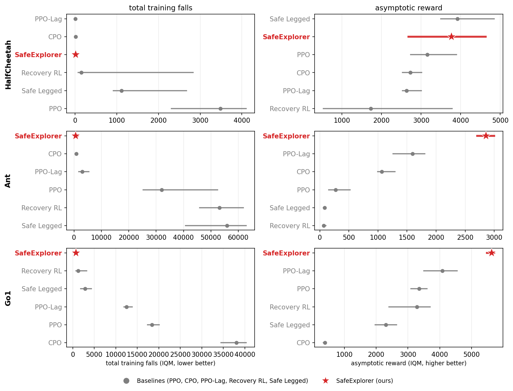
15.2 Per-environment learning curves↩︎
The interval plot summarizes the endpoints; the learning curves show how each method gets there. 4 traces reward and cumulative falls across the full training run, the trajectory view of the headline endpoints just reported.
![Figure 4: Per-environment learning curves: rows are episodic reward and cumulative training-time falls; columns are HalfCheetah, Ant, Go1. Solid = mean across seeds, shaded = [min, max] envelope; curves smoothed with a moving average for display. Recovery-rate curves are deferred to 15.12.](/article/2607.08925/figures/learning_curves_grid.png "fig:")
15.3 Additional ablations↩︎
Having established what the headline shows, we now ask which design choices produce it, starting from the component ablation. 8 analyzes that ablation in the body. 5 gives its reward-vs-falls view, the trade-off complement to the falls-to-success ranking of 1; here we also report the remaining variants. The two threads opened here are picked up in turn below: the soft-gate variants (15.4) help marginally on Ant and hurt on HalfCheetah, and the \(\lambda_{\mathrm{compat}}\) sweep is in 15.5.
![Figure 5: Ablation ladder on the reward-vs-falls plane: PPO and the four rungs, Unmasked PG \to masked learned-V \to masked analytic-V \to SafeExplorer. Markers are rliable interquartile means with 95\% stratified-bootstrap confidence intervals [65]; total training falls on a log axis, upper-left is better (fewer falls, higher reward). The reward-vs-falls view of the variants 1 ranks by falls-to-success; SafeExplorer (red star) is on the Pareto front in every environment.](/article/2607.08925/figures/ladder_pareto.png "fig:")
15.4 Soft compatibility-gate variants↩︎
The body ablation (8, 1) analyzes the clean ablation ladder Unmasked PG \(\to\) masked learned \(V\) \(\to\) analytic \(V\) \(\to\) hard \(C_\theta(\tau)\) (SafeExplorer); 8 tabulates its full numbers. The two soft-gate variants, a soft re-entry-advantage gate \(w_t^{\mathrm{soft}}\) (10 ) applied on the analytic-\(V\) model, and the same soft gate applied on a decomposed value, are negative results. They help marginally on Ant and hurt on HalfCheetah, and never approach SafeExplorer’s safety. We report their full numbers here and omit them from the body ablation to keep it focused on variants that isolate a single design choice. 8 places them alongside the ladder rungs so the off \(\to\) soft \(\to\) hard progression is visible (same five-seed protocol as 1).
| 2-3(lr)4-5(lr)6-7 Method | Reward | Falls | Reward | Falls | Reward | Falls |
| Unmasked PG | \(\mathbf{4922\pm243}\) | \(194\pm40\) | \(1253\pm427\) | \(5177\pm1399\) | \(\mathbf{5788\pm425}\) | \(2936\pm629\) |
| Masked, learned \(V\) | \(1982\pm1058\) | \(306\pm360\) | \(222\pm275\) | \(50011\pm30828\) | \(4374\pm758\) | \(972\pm206\) |
| Analytic \(V\) (no gate) | \(3870\pm447\) | \(73\pm19\) | \(174\pm150\) | \(35481\pm21851\) | \(4473\pm628\) | \(926\pm259\) |
| Soft \(\Ctheta\) gate | \(2645\pm829\) | \(1215\pm1843\) | \(663\pm323\) | \(11745\pm18434\) | \(4142\pm1471\) | \(2044\pm2647\) |
| Soft \(\Ctheta\), decomposed \(V\) | \(3569\pm1074\) | \(721\pm985\) | \(505\pm319\) | \(8183\pm8064\) | \(4374\pm1191\) | \(1242\pm472\) |
| (hard \(\Ctheta\)) | \(3581\pm971\) | \(\mathbf{14\pm8}\) | \(\mathbf{2857\pm129}\) | \(\mathbf{754\pm463}\) | \(5594\pm177\) | \(\mathbf{731\pm177}\) |
4pt
The mechanism behind the soft gate’s failure is given in 4.4: on a failed recovery segment the soft gate still emits a negative-signed imitation pressure, teaching \(\pi_\theta\) to unlearn the recovery action at those states, a noisy signal that the hard gate removes by zeroing the term on failures.
15.5 \(\lambda_{\mathrm{compat}}\) sensitivity (SafeExplorer)↩︎
With the gate fixed, the remaining knob on the regularizer is its weight. We sweep \(\lambda_{\mathrm{compat}}\in \{10^{-4},10^{-3},10^{-2},10^{-1},1.0\}\) on HalfCheetah and Ant.
| \(\lambdaCompat\) | reward | falls | reward | falls |
|---|---|---|---|---|
| \(10^{-4}\) | \(2654\pm1833\) | \(211\pm266\) | \(1803\pm1176\) | \(3557\pm3795\) |
| \(10^{-3}\) | \(4768\pm583\) | \(\mathbf{47\pm41}\) | \(2908\pm157\) | \(428\pm454\) |
| \(10^{-2}\) | \(\mathbf{5783\pm481}\) | \(374\pm548\) | \(\mathbf{3124\pm355}\) | \(639\pm517\) |
| \(10^{-1}\) | \(5288\pm667\) | \(64\pm57\) | \(2281\pm894\) | \(\mathbf{149\pm140}\) |
| \(1.0\) | \(5536\pm333\) | \(137\pm151\) | \(1352\pm1036\) | \(2798\pm5658\) |
3pt
The \(\lambda_{\mathrm{compat}}= 10^{-3}\) row is an independent replication of 1’s configuration: it lands at HalfCheetah \(4768\pm583\) / \(47\pm41\) against 1’s \(3581\pm971\) / \(14\pm8\), consistent within seed noise for a heavy-tailed falls count. The same runs also back 15 (HalfCheetah/Ant).
The optimum is environment-specific. On HalfCheetah the reward peaks sharply at \(\lambda_{\mathrm{compat}}= 10^{-2}\) (\(5783\)). On Ant the reward is within seed noise from \(\lambda_{\mathrm{compat}}= 10^{-3}\) to \(10^{-2}\), with \(10^{-3}\) the safer choice. Both environments are robust within a \(\sim 10\times\) band around the optimum.
The main results use a single \(\lambda_{\mathrm{compat}}= 10^{-3}\). SafeExplorer in 1 and 4 fixes \(\lambda_{\mathrm{compat}}= 10^{-3}\) across all three environments rather than a per-environment optimum. We make this choice on safety grounds. In the sweep above, \(\lambda_{\mathrm{compat}}= 10^{-3}\) attains the lowest HalfCheetah training-fall count (\(47\), against \(374\) at \(10^{-2}\)) and a near-lowest count on Ant. A larger \(\lambda_{\mathrm{compat}}= 10^{-2}\) would raise HalfCheetah reward substantially (\(5783\) vs \(4768\)) and is marginally better on Ant, but it does so at roughly \(8\times\) the HalfCheetah falls. We therefore keep the uniform \(10^{-3}\) default so that the headline fall reductions are not traded away for extra falls, and we note \(10^{-2}\) as the reward-optimal setting for HalfCheetah for practitioners who can tolerate the higher fall count.
15.6 Fixed-\(d\) ablation: the safe-region schedule vs.a constant \(d\)↩︎
With the gate and its weight fixed, the last training-time design choice is the safe-region radius, which SafeExplorer anneals on a curriculum. A natural counterfactual is to pick a smaller \(d_{\max}\) and hold \(d\) constant there. 10 sweeps fixed \(d \in \{0.25, 0.5, 0.75, 1.0\}\cdot d_{\max}\) on each of the three environments, with otherwise-identical SafeExplorer.
| \(d/\dmax\) | |||
|---|---|---|---|
| \(25\%\) | \(3344\pm1642 / 1189\pm1274\) | \(990\pm2 / \mathbf{5\pm4}\) | \(2898\pm147 / 1895\pm409\) |
| \(50\%\) | \(2476\pm668 / 2623\pm664\) | \(1602\pm463 / 5522\pm1505\) | \(5423\pm119 / \mathbf{397\pm33}\) |
| \(75\%\) | \(\mathbf{3629\pm582} / 3489\pm889\) | \(555\pm178 / 19941\pm4063\) | \(5572\pm179 / 888\pm372\) |
| \(100\%\) | \(3535\pm1053 / 3632\pm641\) | \(565\pm301 / 21837\pm8376\) | \(\mathbf{5752\pm158} / 1662\pm272\) |
| (, ref.) | \(\dmax{=}2.0\):\(3581\pm971 / \mathbf{14\pm8}\) | \(\dmax{=}0.4\):\(\mathbf{2857\pm129} / 754\pm463\) | \(\dmax{=}0.15\):\(5594\pm177 / 731\pm177\) |
4pt
HalfCheetah. Every fixed-\(d\) cell pays \(\sim 1{,}200\) to \(3{,}600\) training falls and tops out near \(2{,}500\) to \(3{,}600\) reward, while the linear-curriculum reference reaches \(3{,}581\) reward at only \(14\) falls (an \(85\times\) to \(260\times\) falls advantage). No constant \(d\) matches the curriculum’s reward-at-low-falls. The small-\(d\) cells stay safer but low-reward and the large-\(d\) cells climb in falls without gaining reward.
Ant. The smallest fixed-\(d\) (p25, \(d=0.1\)) is very safe (\(5\) falls) but useless (\(990\) reward). Larger constant \(d\) accumulates \(5{,}500\) to \(21{,}800\) falls without reaching the curriculum’s reward. The linear curriculum gets \(2857\) reward at \(754\) falls, which no constant \(d\) matches.
Go1. On Go1 the comparison is closer, and the curriculum does not strictly dominate. A tuned constant \(d\) is competitive. Fixed-\(d\)-p50 (\(5423 / 397\)) attains essentially the curriculum’s reward (\(5594\)) at fewer falls (\(397\) vs \(731\)), and p75 and p100 trade modest extra falls for similar reward. The curriculum’s value on Go1 is therefore robustness to the choice of \(d\), it reaches high reward at low falls without a per-environment \(d\) search, rather than a strict win over the best constant \(d\).
Summary. On HalfCheetah and Ant no constant \(d\) matches the schedule’s high reward at comparable safety. On Go1 a tuned fixed-\(d\) (p50) is competitive on both axes, so there the schedule’s contribution is sparing the practitioner a per-environment \(d\) search rather than a strict dominance. The safe-region schedule is a supporting mechanism for the objective-gap bound (2). The method’s correctness rests on the unbiased masked gradient (1), not on the schedule.
15.7 Curriculum-schedule sensitivity (SafeExplorer on Ant)↩︎
| Schedule | Reward | Falls |
|---|---|---|
| Linear | \(\mathbf{2888\pm351}\) | \(\mathbf{952\pm1121}\) |
| Log | \(\mathbf{2906\pm374}\) | \(1086\pm438\) |
| Step (4 jumps) | \(1537\pm549\) | \(5998\pm2788\) |
| Constant (\(d=\dmax\)) | \(294\pm74\) | \(29855\pm4747\) |
Granting that some schedule beats a constant \(d\), the next question is which one. 11 reports three alternatives against the linear default. Linear and log are tied within seed noise on every metric. The step schedule is worse on both, with lower reward and \(6\times\) more falls. Constant-\(d\) (no curriculum) collapses, accumulating \(31\times\) the falls of the linear curriculum at a tenth of its reward. This is consistent with the fixed-\(d\) ablation above (15.6), whose constant \(d{=}d_{\max}\) cell shows the same qualitative collapse (at the body radius rather than this table’s wider one), and with the prediction of 2 that the gap closes as \(\beta\) shrinks, which the curriculum drives.
15.8 Compute-scaling: \(2\times\) matched-budget on HalfCheetah and Ant↩︎
| Method | Main (\(8\)M) | \(2\times\) (\(16\)M) | |
|---|---|---|---|
| PPO | \(3163\pm966 / 5266\pm2539\) | \(3590\pm1969 / 15112\pm8500\) | |
| \(\mathbf{4027\pm1239 / 248\pm281}\) | \(\mathbf{5912\pm881 / 217\pm340}\) | ||
| PPO | \(296\pm35 / 32369\pm5625\) | \(197\pm92 / 88900\pm35552\) | |
| \(\mathbf{2888\pm351 / 952\pm1121}\) | \(\mathbf{2950\pm419 / 3332\pm2620}\) |
r0.62 3pt
With the design choices settled, we turn to whether the chosen configuration holds up under conditions the body did not exercise, starting with more compute. We re-run PPO and SafeExplorer at \(2\times\) the main budget (\(8\mathrm{M}\to16\mathrm{M}\)) on HalfCheetah and Ant(12; wider radii than the body protocol, see the caption). SafeExplorer’s reward improves or holds with \(2\times\) compute (HalfCheetah\(4027\to5912\), Ant\(2888\to2950\)) while its falls stay low. PPO’s falls instead grow sharply (HalfCheetah\(\sim 2.9\times\), Ant\(\sim 2.7\times\)), so the safety gap widens with budget rather than closing. Re-tuning \(d_{\max}\) for longer horizons or a multi-stage curriculum is left to follow-up work.
15.9 Compatibility-regularizer normalization (global vs.per-segment)↩︎
| Env | global (default) | per-segment |
|---|---|---|
| \(4027\pm1239 / 248\pm281\) | \(\mathbf{5030\pm664 / 48\pm36}\) | |
| \(\mathbf{2888\pm351 / 952\pm1121}\) | \(2474\pm489 / 2625\pm1583\) |
The \(C_\theta(\tau)\) loss in 7 averages across all recovery-active timesteps in the current minibatch (“global”). An alternative “per-segment” normalization averages within each
contiguous safe\(\to\)unsafe\(\to\)safe segment, then over segments, which prevents long unsafe excursions from dominating the loss. 13 reports both on
HalfCheetah and Ant. Per-segment helps on HalfCheetah(higher reward, fewer falls) but hurts on Ant(lower reward, more falls). With
no consistent winner across environments and the means within roughly one standard deviation, we keep global as the simpler default.
15.10 Action-noise robustness (HalfCheetah SafeExplorer)↩︎
| \(\sigma_a\) | Reward | Falls |
|---|---|---|
| \(0.00\) | \(4027\pm1239\) | \(248\pm281\) |
| \(0.05\) | \(4482\pm419\) | \(108\pm73\) |
| \(0.10\) | \(2346\pm964\) | \(546\pm395\) |
A second stress axis perturbs the actions themselves. We re-train SafeExplorer on HalfCheetah with Gaussian action noise of standard deviation \(\sigma_a \in \{0.0, 0.05, 0.10\}\) added to every action (recovery and main) at the \(\lambda_{\mathrm{compat}}= 10^{-3}\) default (14). Reward and falls stay within seed noise up to \(\sigma_a = 0.05\), then degrade at \(\sigma_a = 0.10\) (\(-42\%\) reward, more than double the falls). An action-noise sweep at the HC-tuned \(\lambda_{\mathrm{compat}}= 10^{-2}\) is left to follow-up work. We also ran \(\sigma_a = 0.20\) as a stress test. SafeExplorer collapses (\(1863\pm542\) reward, \(1659\pm1807\) falls) when the injected noise is comparable in scale to the recovery’s action magnitude, and we omit it from the table as a known out-of-regime failure mode.
15.11 Failure-mode catalog↩︎
The stress tests above probe how the chosen configuration degrades; this catalog records the qualitative failure each rejected variant exhibits, so the quantitative gaps in the ablations have a concrete behavioral reading.
PPO on Go1: agent falls within first 200 steps; recovery is unavailable; episode terminates.
Analytic-\(V\) variant on Ant: agent learns to balance briefly but never escapes the recovery policy’s basin; \(\alpha\) stays near 1 for the full training run.
Soft-gate variant on HalfCheetah: regularizer fits failed-recovery actions; reward oscillates; final policy is unreliable.
SafeExplorer on Ant: clean separation, \(\alpha\) drops to near zero around update 1000, reward climbs steadily thereafter, falls plateau.
15.12 Empirical check of 2↩︎
We now turn from the method’s empirical robustness to its theory, checking each of the paper’s two theorems against the runs, starting with the objective-gap bound. 2 bounds the deployment gap \(|J^{\mathrm{mix}}(\theta_k) - J(\theta_k)|\), between the during-training mixed-policy return and the return of \(\pi_\theta\) deployed alone, by the main-policy out-of-region rate \(\beta(\theta, d)\). The bound is a proportionality, not a vanishing guarantee. It predicts a small gap exactly when \(\beta(\theta, d)\) is small, and 3 sharpens this to an exact fixed point only in the idealized \(\beta(\theta, d)\to 0\) limit. We test that prediction directly. Every 4 PPO updates we run a recovery-disabled evaluation pass, averaging \(5\) episodes per pass, that samples from the same stochastic policy \(\pi_\theta(\cdot|s) = \mathcal{N}(\mu_\theta(s), \sigma_\theta^2)\) used in training, the operative \(J(\theta_k)\), and compare it to the mixed-policy rollout return \(J^{\mathrm{mix}}(\theta_k)\). Because \(\beta(\theta, d)\) is an out-of-region rate under \(\pi_\theta\) alone and is not directly observable, we report alongside it the observable recovery rate \(\alpha\), which 4.2 identifies as a diagnostic for \(\beta(\theta, d)\) rather than a certified upper bound. A deterministic pass using \(\mu_\theta(s)\) alone is also logged as a noise-reduced deployment diagnostic but is not the quantity the theorem concerns.
| Env | \(J^{\mathrm{mix}}\) | \(J\) | \(J^{\mathrm{mix}} - J\) | \(\alpha\) | Falls (train) | Falls (eval/ep) |
|---|---|---|---|---|---|---|
| \(4677 \pm 542\) | \(4676 \pm 552\) | \(0 \pm 12\) | \(0.000\) | \(47 \pm 41\) | \(0.00\) | |
| \(2904 \pm 145\) | \(2921 \pm 151\) | \(-17 \pm 25\) | \(0.000\) | \(428 \pm 454\) | \(0.12\) | |
| \(5576 \pm 213\) | \(5112 \pm 340\) | \(463 \pm 150\) | \(0.044 \pm 0.005\) | \(768 \pm 241\) | \(0.36\) |
4pt
The result follows the bound’s structure precisely, and the key observation is that the gap tracks \(\beta(\theta, d)\). On HalfCheetah and Ant the recovery rate falls to essentially zero (\(\alpha = 0.000\) on both at end-of-training), and the gap closes to within seed noise of zero (\(0 \pm 12\) and \(-17 \pm 25\)). These are the self-stable environments. Here \(\pi_\theta\) holds the safe region unaided, so \(\pi^{\mathrm{mix}}_\theta\equiv \pi_\theta\) along the trajectory, \(\beta(\theta, d)\to 0\), and the fixed point of 3 is reached up to the invariance-slack residual \(\eta_\star\) the corollary anticipates (the residuals here are statistically indistinguishable from zero; empirically it is the stochastic policy’s entropy floor that keeps \(\eta_\star\) from being exactly zero). On Go1 the policy does not become fully self-stable, because the quadruped’s gait cannot stay inside the tight \(\mathcal{R}(d_{\max})\) tube. The recovery rate therefore settles at a small positive floor (\(\alpha = 0.044 \pm 0.005\)) rather than at zero, and the gap settles at a correspondingly positive residual (\(463 \pm 150\), about \(8\%\) of \(J^{\mathrm{mix}}\)) rather than vanishing. After the early-curriculum transient the gap collapses from its peak on HalfCheetah, stays within seed noise of zero on Ant in the final average despite a late upward drift in the plotted per-seed magnitude, and declines but stays positive on Go1(6). On Go1 it falls from \(\sim 1950\) when the safe region is small to a small positive residual at \(16\)M env-steps. The end-of-training gap and recovery rate in 15 make the proportionality explicit. The gap is near zero exactly where \(\alpha\) is, and the only environment with a residual gap is the only one with a residual \(\alpha\).
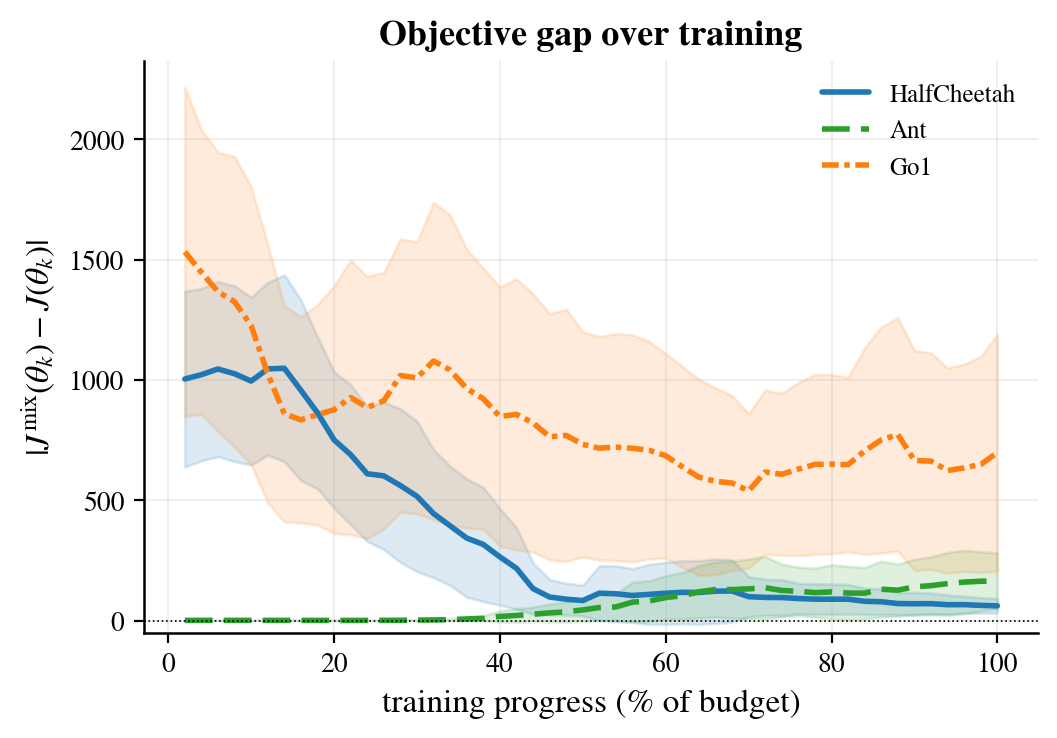
This two-regime behavior is a stronger test of 2 than a uniform collapse to zero would be. The bound does not assert that the gap vanishes; it asserts that the gap is governed by \(\beta(\theta, d)\). HalfCheetah and Ant realize the vanishing regime (\(\beta(\theta, d)\to 0\)), and Go1 realizes the residual regime (\(\beta(\theta, d)\) bounded away from zero because 2 holds only approximately for a quadruped confined to a tight tube), with the observable \(\alpha\) moving in lockstep with the gap in both. The sign of the gap is itself interpretable. On Go1, \(J^{\mathrm{mix}} - J > 0\) means that deploying \(\pi_\theta\) alone forfeits the return that the recovery policy would otherwise secure, so the gap measures the policy’s residual reliance on the recovery policy, which HalfCheetah and Ant drive to zero and Go1 reduces to about \(8\%\).
The absolute prefactor of 2 (\(2r_{\max}/(1-\gamma)^2 \approx 2 \times 10^5\) for \(r_{\max}= 10\), \(\gamma = 0.99\)) is loose, as is standard for performance-difference-lemma bounds, so we do not read the inequality quantitatively. Its operative content is the structural claim that any mechanism reducing \(\beta(\theta, d)\), here the radius curriculum together with the compatibility regularizer, tightens the gap. 6 confirms that claim across the full range of \(\beta(\theta, d)\) our three environments realize. Eval-time falls under \(\pi_\theta\) alone (recovery disabled) corroborate the reading. They are \(0.00\), \(0.12\), and \(0.36\) per episode on HalfCheetah, Ant, and Go1, ordered exactly as the gaps and the recovery rates are. 7 plots the full recovery-rate trajectories that this diagnostic summarizes.
![Figure 7: Recovery rate \alpha (fraction of rollout steps on which recovery fired) over training, per environment, for the recovery-using methods (the CMDP solvers act with a single policy and never invoke recovery, so they have no \alpha). Solid = mean across seeds, shaded = [min, max] envelope.](/article/2607.08925/figures/alpha_curves_appendix.png "fig:")
15.13 Masked gradient versus IS under a stochastic recovery↩︎
With the objective-gap bound checked, we turn to the gradient estimator: 1 makes the masked estimator exactly unbiased at recovery steps, while per-step IS, where it applies at all, is biased in general (1); what remains empirical is how the two compare in practice. 1 holds for any \(\theta\)-independent recovery; for a deterministic one, not even IS applies (4.1). Here we ask what happens when the recovery is stochastic, so IS becomes an option. Writing \(w_t = \pi_\theta(a_t \mid s_t) / \pi^{\mathrm{rec}}(a_t \mid s_t)\) for the importance weight at a recovery step, the IS estimator of \(\nabla_\theta J^{\mathrm{mix}}(\theta)\) (1) decomposes as \[\hat{g}_{\mathrm{IS}} = \underbrace{\sum_{t :\, s_t \in \mathcal{R}} \nabla_\theta \log \pi_\theta(a_t\mid s_t)\, A_t}_{\hat{g}_{\mathrm{masked}}} \;+\; \sum_{t :\, s_t \notin \mathcal{R}} w_t\, \nabla_\theta \log \pi_\theta(a_t\mid s_t)\, A_t, \label{eq:is-decomp}\tag{11}\] with \(A_t\) the PPO advantage estimate. The second sum would be mean zero by the score-function identity only if \(A_t\) were replaced by an action-independent baseline \(b(s_t)\); with the actual advantage, which depends on \(a_t\) through the reward and the successor state, its conditional mean is the off-policy policy-gradient contribution at the unsafe states, which is generically nonzero. The per-step IS estimator is therefore biased for \(\nabla_\theta J^{\mathrm{mix}}\), and masking removes a bias-carrying term, not merely a noisy one. A recovery policy differs sharply from the main policy by design, so the term’s weights are heavy-tailed; truncating them [31], [32] trades variance for further bias. The measurement below therefore compares two estimators that do not share a mean: the recorded explosion of the IS weights is evidence about the conditioning of the added term, not a like-for-like variance comparison between unbiased estimators.
Concretely, we rerun SafeExplorer on all three environments (settings of 6) with the recovery action sampled from the SAC recovery rather than taken greedily at its mean, and shadow-compute, per rollout, the weights’ effective sample size and each estimator’s gradient variance. Training itself always uses the masked gradient.
8 shows that the three regimes expose complementary failure modes. On HalfCheetah the strong recovery makes the weights degenerate from the first update. The effective sample size never exceeds \(0.5\%\) of the recovery steps, and the IS gradient variance exceeds the masked variance by a factor of up to \(8\times10^{12}\). On Ant the weak recovery initially overlaps the main policy and IS stays formally usable for longer, but the variance ratio holds near \(10^{13}\) for the first \(1.2\)M steps. Go1 completes the spectrum. Over its 12-dimensional action space the recovery’s actions are so unlikely under the main policy that the weights die at once (effective sample size always below \(3\%\), reaching \(7\times10^{-5}\)), so the added term vanishes before its variance can build, and the ratio never rises above \(\sim\!40\) and sits at one for the full \(16\)M steps, over which the quadruped’s recovery rate never reaches zero (15.12). Once the main policy separates from the recovery the weights vanish and the ratio returns to one. IS proves either catastrophically noisy or identical to the masked estimator, never better in any regime we measure.
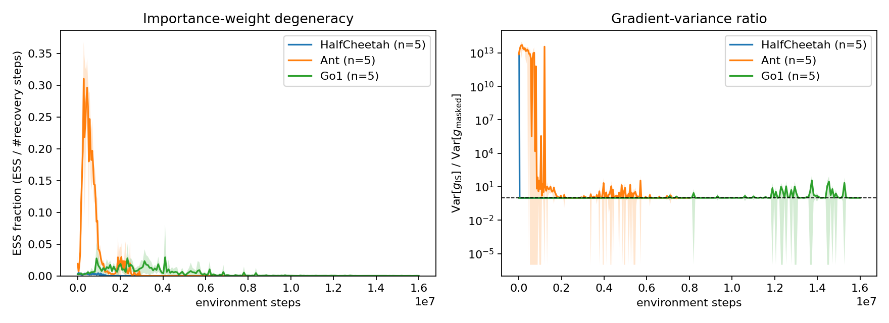
Training with the truncated-IS gradient (\(w_t\) clipped at \(c = 10\)) confirms the cost (9). These runs use the sampled-recovery setup of this appendix, so their absolute rewards are not comparable to 1’s greedy-recovery numbers; only the within-setup masked-vs-IS differences are meaningful. On HalfCheetah the weights die immediately and the two variants are statistically indistinguishable (reward \(4675 \pm 642\) versus \(4421 \pm 647\)). On Ant the million-step degeneracy window is expensive: \(793 \pm 214\) reward against \(1325 \pm 289\) for the masked gradient, a \(40\%\) drop, and its lower fall count (\(2066 \pm 1582\) versus \(4682 \pm 1047\)) reflects the weaker policy rather than safer behavior. On Go1 the truncated-IS variant again trails the masked gradient (\(4884 \pm 241\) versus \(5243 \pm 219\) reward, a \(7\%\) drop) at statistically indistinguishable falls (\(3293 \pm 589\) versus \(3401 \pm 351\)).
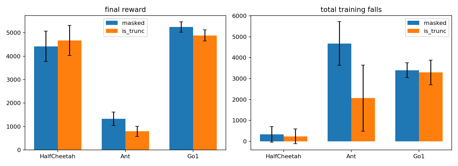
15.14 CMDP baselines: constraint feasibility↩︎
Having checked the method’s own theory, we finally audit the baselines it is compared against, asking whether the CMDP solvers even satisfy the constraint they are given. This
appendix supports the CMDP comparison of 7.3. For the comparison to be fair, both solvers use the OmniSafe implementation [64] and run on the identical environments, reward functions, network architecture, optimizer, and step budget as the variants in 1. We use the direct cost encoding, a cost of \(1\) on a fall (a termination), the actual safety signal the constraint should bound. The only incidental differences from SafeExplorer are
observation and reward normalization, applied to the CMDP baselines and not to SafeExplorer, so they favor the baselines. Reported rewards for both solvers are the raw episode return
(EpRet in OmniSafe), un-normalized and therefore on the same task-reward scale as the other methods. The normalization affects only the solvers’ internal optimization, not the reported numbers.
On this matched footing, 16 reports the final episodic cost each solver converges to, against the cost budget of \(0.05\) it was given (a per-episode fall rate), averaged over the same seeds. The pattern is clean. Both solvers reach feasibility on HalfCheetah, where staying safe is easy, and both fail to reach feasibility on Ant and Go1, where the converged cost exceeds the budget by up to \(19\times\). The poor safety of the CMDP baselines is therefore not a tuning artifact. The constrained optimization does not find a feasible policy at all in the regimes where the safe-region intervention is needed.
| Method | |||
|---|---|---|---|
| CPO | \(0.007\pm0.011\) | \(0.103\pm0.029\) | \(0.956\pm0.025\) |
| PPO-Lagrangian | \(0.001\pm0.001\) | \(0.326\pm0.177\) | \(0.377\pm0.126\) |
A safe-region indicator cost (cost \(1\) at every step outside \(\mathcal{R}(d_{\max})\)) is a second natural encoding, but it is comparable to the recovery-using methods only when the recovery policy is active, since that is the setting in which an out-of-region penalty reduces to recovery-active reward shaping. We therefore report the direct termination encoding in the main comparison and leave the recovery-active safe-region variant to future work.
16 Broader Impact↩︎
The goal of this work is to make reinforcement learning on physical robots safer to train. Achieving that goal would reduce hardware damage during training, lower the experimental cost borne by robot-learning research groups, and provide a foundation for on-robot continual learning that does not depend on extensive pre-training in simulation.
Set against that intent, the dual-use surface of the technique is narrow. It is dual-use only in the trivial sense that any improvement in robotic control technology is so, because the method does not change the capabilities a deployed policy can express, only the training-time safety profile of how that policy is reached. For this reason we do not foresee specific misuse pathways introduced by this work that are not already present in the underlying PPO + SAC + MuJoCo / Go1 stack.
The experiments themselves are deliberately scoped to limit any training-time harm. We do not collect or release human-subject data and do not perform experiments that could affect bystanders during training. All experiments are in simulation (MuJoCo and the Go1 model), so the training-time falls we reduce are simulated rather than physical; carrying that reduction onto hardware is future work (9).
Because the contribution is methodological, its value depends on being reproducible and affordable, and we account for both: the full algorithm, hyperparameter, and environment specifications needed to rerun the experiments are given in [app:algorithm,app:hyperparams,app:env]. We report negative results alongside the positive ones, the soft-gate variants, the fixed-\(d\) concessions, and the action-noise stress failures ([app:soft-variants,app:fixed-d,app:failure-modes]), so that future work can avoid repeating them. The compute budget for the component ablation (\(9\) variants \(\times\) \(3\) environments \(\times\) \(5\) seeds, 4 cores each, weighted by per-environment wall-clock) is approximately \(3{,}700\) CPU-core-hours, modest relative to contemporary safe-RL benchmarks; the additional sensitivity sweeps in 15 add further compute.
References↩︎
[thm:gradient,thm:convergence] hold for any bounded reward, covering this training-signal convention; the induced train-to-deploy return gap is controlled by the same \(\beta(\theta, d)\) (11). Reported returns always use the unmodified task reward (6).↩︎