LieBN: Batch Normalization over Lie Groups
June 13, 2026
1 Introduction↩︎
![Figure 1: Illustration of LieBN on the SPD, rotation, and correlation Lie groups. The 2 \times 2 SPD, 3 \times 3 rotation, and 3 \times 3 correlation manifolds can be embedded into \mathbb{R}^3 as an open cone [1], a closed ball with antipodal points identified [2], and an open elliptope [3], respectively. LieBN is illustrated by (1) the left-invariant AIM and the proposed right-invariant CRIM geometry on the SPD manifold, (2) left or right translation under a bi-invariant metric on the rotation manifold, and (3) the bi-invariant ECM and LSM geometry on the correlation manifold. On the SPD and correlation manifolds, the batch mean and variance of the same input samples differ under different geometries. In all sub-figures, the black, blue, green, and red dots denote the boundary of the space, the input Lie group samples, the normalized samples, and the batch mean, respectively. As illustrated, our LieBN effectively normalizes the Lie group distribution.](/article/2607.08783/Figs/LieBN_illustration.png "fig:")
Over the past decade or so, Deep Neural Networks (DNNs) have achieved significant progress across various scientific fields [4]–[7]. Traditionally, DNNs have been developed under the assumption that the latent space of the input data is Euclidean. However, many applications involve non-Euclidean structures, such as manifolds [8]. To address this challenge, researchers have extended various types of DNNs to manifolds, based on the theories of Riemannian geometry [9]–[27].
Motivated by the great success of normalization techniques [28]–[31], researchers have sought to devise normalization layers tailored for manifold-valued data. Brooks et al[32] introduced Riemannian Batch Normalization (RBN) designed specifically for the Symmetric Positive Definite (SPD) manifold, with the ability to normalize the Riemannian mean. Kobler et al[33] extended this approach to further control the Riemannian variance. However, the above methods are constrained within the Affine-Invariant Metric (AIM) on the SPD manifold, limiting their applicability. On the other hand, Chakraborty [34] proposed two distinct Riemannian normalization frameworks: one for Riemannian homogeneous spaces [34] and another for matrix Lie groups [34]. Nonetheless, the normalization designed for Riemannian homogeneous spaces cannot normalize mean nor variance, while the one for matrix Lie groups is confined to a specific type of distance [34]. Meanwhile, Luo [35] proposed an RBN layer for general geometries. However, similar to [34], it lacks theoretical guarantees for normalizing sample statistics. Therefore, a principled Riemannian normalization framework capable of controlling both Riemannian mean and variance remains unexplored.
Given that Batch Normalization (BN) [28] serves as the foundational prototype for various types of normalization, our paper focuses on RBN, with the potential to be extended to other normalization variants. Since several manifold-valued measurements form Lie groups, such as Symmetric Positive Definite (SPD) manifolds [3], [36], [37], special orthogonal groups \(\mathrm{SO}(n)\) [38], and full-rank correlation matrices [3], [39], we further direct our attention to Lie groups. As each Lie group naturally admits left- and right-invariant metrics [40], we propose a principled framework for RBN over Lie groups under invariant metrics, referred to as LieBN. Compared to previous work, our framework provides a theoretical guarantee for normalizing the Riemannian sample mean and variance across general Lie groups.
Empirically, we focus on the SPD, special orthogonal, and full-rank correlation manifolds. On SPD manifolds, we generalize three existing Lie group structures into parameterized ones by matrix power deformation. Additionally, we propose a novel right-invariant metric, which, to the best of our knowledge, is the first non-trivial right-invariant SPD metric1, referred to as Cholesky Right Invariant Metric (CRIM). We then instantiate our LieBN framework on SPD manifolds under these four Lie group structures. For rotation matrices, we adopt the popular bi-invariant metric [38], which will induce two types of LieBN: one w.r.t. left-invariance and another w.r.t. right-invariance. On the correlation manifold, we manifest our LieBN under four recently developed correlation geometries [3], [39]. Besides, we discuss the optimization of the involved correlation-valued parameters. To facilitate usage, we provide a LieBN toolbox compatible with PyTorch, which can be used as a drop-in module. 1 illustrates our LieBN on different geometries, while 2 illustrate a minimal demo. Extensive experiments on SPD, rotation, and correlation manifolds across three tasks—radar recognition, human action recognition, and electroencephalography (EEG) classification—demonstrate the effectiveness of our methods.
None
Figure 2: Minimal examples of applying LieBN..
We emphasize that our work is fundamentally distinct from [32], [33], [35] in theory and more general than [34]. Previous RBN methods are either designed for specific geometries [32]–[34] or fail to control both the mean and variance [35]. In contrast, our LieBN ensures the normalization of both the mean and variance across general Lie groups. In summary, our main contributions are:
A general Lie group batch normalization framework with controllable first- and second-order moments;
A novel right-invariant metric on the SPD manifold, which is the first non-trivial right-invariant SPD metric;
Concrete instantiations of our LieBN framework on different geometries: four on SPD manifolds, one on the rotation matrices, and four on the correlation manifold;
Validation of effectiveness of our LieBN framework by extensive experiments on different geometries.
This paper extends our previous conference paper [41] in both theory and implementation. Theoretically, the original LieBN framework was restricted to Lie groups under a left-invariant metric. However, Lie groups also naturally admit right-invariant metrics, which share many theoretical properties with left-invariant ones. Therefore, we generalize LieBN to all natural invariant metrics, including left-, right-, and bi-invariant metrics, providing a more comprehensive framework for RBN. Additionally, we propose a novel non-trivial right-invariant metric on the SPD manifold. In terms of implementation, beyond the original applications to SPD and rotation matrices, we further manifest LieBN on four correlation geometries. Besides, the previous LieBN on \(\mathrm{SO}(3)\) was based solely on left-invariance and validated on a small dataset. In contrast, this journal submission expands the implementation to both left- and right-invariance and conducts extensive experiments across multiple datasets.
2 Preliminaries↩︎
This section briefly reviews Lie groups, as well as the concrete Lie groups of SPD, rotation, and full-rank correlation matrices. For more in-depth discussions, we refer the reader to [42] for smooth manifolds, [40], [43] for Riemannian manifolds, and [44] for Lie groups.
2.1 Lie Groups↩︎
Definition 1 (Lie Groups [42]). A manifold \(\mathcal{M}\) is a Lie group, if it forms a group with a group operation \(\odot\) such that \(m(\cdot,\cdot): \mathcal{M}\times \mathcal{M}\ni (x,y) \to x \odot y \in \mathcal{M}\) and the group inverse \(i(\cdot): \mathcal{M}\ni x \to x_{\odot}^{-1} \in \mathcal{M}\) are both smooth.
Definition 2 (Invariance [40]). A Riemannian metric \(g^{\mathrm{L}}\) over a Lie group \(\{\mathcal{M}, \odot\}\) is left-invariant, if for any \(x,y \in \mathcal{M}\) and \(V_1,V_2 \in T_x\mathcal{M}\), it satisfies \(g^{\mathrm{L}}_y(V_1,V_2) = g^{\mathrm{L}}_{\operatorname{L}_x(y)} \left(\operatorname{L}_{x*,y}(V_1), \operatorname{L}_{x*,y}(V_2) \right)\), with \(\operatorname{L}_x(y) = x \odot y\) as the left translation by \(x\), and \(\operatorname{L}_{x*,y}\) as the differential map of \(\operatorname{L}_x\) at \(y\). Similarly, a right-invariant metric \(g^{\mathrm{R}}\) satisfies \(g^{\mathrm{R}}_y(V_1,V_2) = g^{\mathrm{R}}_{\operatorname{R}_x(y)} \left(\operatorname{R}_{x*,y}(V_1), \operatorname{R}_{x*,y}(V_2) \right)\), with \(\operatorname{R}_x(y) = y \odot x\) as the right translation by \(x\), and \(\operatorname{R}_{x*,y}\) as the differential at \(y\).
A Lie group is both a group and a manifold. The most natural Riemannian metric on a Lie group is the left- or right-invariant metric2. A bi-invariant metric has both left- and right-invariance. In this paper, \(\{\mathcal{M}, \odot, g\}\), abbreviated as \(\mathcal{M}\), always denotes a Lie group with an invariant metric.
The idea of pullback is ubiquitous in differential geometry and can be viewed as a natural counterpart of the bijection.
Definition 3 (Pullback Metrics [43]). Suppose \(\mathcal{M}_1,\mathcal{M}_2\) are smooth manifolds, \(g\) is a Riemannian metric on \(\mathcal{M}_2\), and \(f:\mathcal{M}_1 \rightarrow \mathcal{M}_2\) is a diffeomorphism. The pullback of \(g\) by \(f\) is defined point-wisely as \((f^*g)_p(V,W) = g_{f(p)}(f_{*,p}(V),f_{*,p}(W))\), where \(f_{*,p}(\cdot)\) is the differential map of \(f\) at \(p \in \mathcal{M}_1\), and \(V,W \in T_p\mathcal{M}_1\). \(f^*g\) is a Riemannian metric on \(\mathcal{M}_1\), called the pullback metric of \(g\) by \(f\).
Although pullback metrics can also be defined by smooth map [43], we focus on the diffeomorphism. Additionally, if \(\{\mathcal{M}_2, \odot_2 \}\) forms a Lie group, the diffeomorphism \(f\) can pull back the group operation \(\odot_2\) to \(\odot_1\) on \(\mathcal{M}_1\): \[\label{eq:group95iso} P \odot_1 Q = f^{-1}(f(P) \odot_2 f(Q)), \forall P, Q \in \mathcal{M}_1.\tag{1}\]
Definition 4 (Weighted Fréchet Mean & Variance [45]). Let \(\{w_{1 \ldots N}\}\) be weights satisfying a convexity constraint, i.e., \(\forall i, w_i>0\) and \(\sum_i w_i=1\). The weighted Fréchet mean (WFM) of a set of manifold-valued points \(\{ P_{i \ldots N} \in \mathcal{M} \}\) is defined as \[\label{eq:wfm95spd} \operatorname{WFM}\left( \{w_i\}, \{P_{i} \} \right) = \underset{M \in \mathcal{M}}{\operatorname{argmin}} \sum\nolimits_{i=1}^N w_i\operatorname{d}^2\left(P_i, M \right),\tag{2}\] where \(\operatorname{d}(\cdot,\cdot)\) denotes the geodesic distance. When \(w_i=\frac{1}{N}\) for all \(i\), 2 is reduced to the Fréchet mean, denoted as \(\operatorname{FM}(\{P_{i} \})\). The Fréchet variance \(v^2\) is the attained value at the minimizer of the Fréchet mean.
On Riemannian manifolds, WFM uniquely exists when samples are locally distributed [46], which are detailed in 9.1 for completeness. In this paper, we always assume the Fréchet batch mean exists. As we focus on Riemannian manifolds, we will use the terms "Riemannian mean" and "Fréchet mean" interchangeably, as well as "Riemannian variance" and "Fréchet variance."
Basic notations. For Euclidean spaces, we denote \(\left\langle \cdot, \cdot\right \rangle\) as the canonical inner product over \(\mathbb{R}^{n \times n}\), with \(\left\|{\cdot} \right\|_\mathrm{F}\) as the induced norms, i.e., \(F\)-norm for matrices. For manifold \(\mathcal{M}\), we denote \(\operatorname{Log}_P\), \(\operatorname{Exp}_P\), and \(\left\langle \cdot, \cdot\right \rangle_{P}=g_P(\cdot,\cdot)\) as the Riemannian logarithm, exponentiation, and metric at \(P \in \mathcal{M}\), respectively. Besides, \(\gamma_{(P,Q)}(t)\) is the geodesic connecting \(P\) and \(Q\) with geodesic distance as \(\operatorname{d}(\cdot,\cdot)\). We provide a complete table of notations in 8.
2.2 SPD Lie Groups↩︎
The SPD manifold has shown great success in diverse applications [9], [14], [33], [47]–[49]. We denote \(n \times n\) SPD matrices as \(\mathcal{S}^{n}_{++}\) and \(n \times n\) real symmetric matrices as \(\mathcal{S}^{n}\). As shown by Arsigny et al [36], \(\mathcal{S}^{n}_{++}\) forms an open submanifold of the Euclidean space \(\mathcal{S}^{n}\), known as the SPD manifold. SPD manifolds exhibit three Lie group structures, each associated with an invariant metric. These metrics include the Log-Euclidean Metric (LEM) [36], Affine-Invariant Metric (AIM) [50], and Log-Cholesky Metric (LCM) [37]. We denote LEM and AIM as \((\alpha,\beta)\text{-LEM}\) and \((\alpha,\beta)\text{-AIM}\), as they are induced by the following \(\mathrm{O}({n})\)-invariant inner product on the tangent space at the identity matrix [51]: \[\label{eq:oim95sym} \langle V,W \rangle^{(\alpha,\beta)}=\alpha \langle V,W \rangle + \beta \operatorname{tr}(V)\operatorname{tr}(W),\tag{3}\] where \(V,W \in T_I\mathcal{S}^{n}_{++} \cong \mathcal{S}^{n}\), and \((\alpha,\beta) \in \mathbf{ST}= \{(\alpha,\beta) \in \mathbb{R}^2 \mid \min (\alpha, \alpha+n \beta)>0\}\). 1 summarizes the Lie structures on SPD manifolds with the following notations. Let \(P, Q \in \mathcal{S}^{n}_{++}\) be SPD matrices. We denote the matrix logarithm, exponentiation, and Cholesky decomposition by \(\operatorname{log}(\cdot)\), \(\operatorname{exp}(\cdot)\), and \(\operatorname{Chol}(\cdot)\), respectively. The Cholesky factors of \(P\) and \(Q\) are \(L=\operatorname{Chol}(P)\) and \(K=\operatorname{Chol}(Q)\). \(\lfloor \cdot \rfloor\) returns the strictly lower triangular part of a square matrix. Other Riemannian operators are summarized in 9.3.
| Metric | \(Q \odot P\) | Invariance | |
|---|---|---|---|
| \(\biparamAIM\) | \(KPK^\top\) | Left-invariance | |
| \(\biparamLEM\) | \(\mexp(\mlog(P)+\mlog(Q))\) | Bi-invariance | |
| LCM | \(\chol^{-1}(\lfloor L + K \rfloor + \bbK \bbL)\) | Bi-invariance |
For \((\alpha,\beta)\text{-LEM}\) and LCM, the Fréchet mean admits a closed-form expression. Moreover, since \((\alpha,\beta)\text{-AIM}\) has non-positive sectional curvature [51], the WFM is a global operation [52] and can be computed by the Karcher flow algorithm [53].
2.3 Rotation Lie Groups↩︎
The set of \(n \times n\) rotation matrices form a Lie group, known as special orthogonal groups, dented as \(\mathrm{SO}(n)\) [42]. Its group operation is the matrix product, with the identity matrix as the neutral element. Any tangent vector \(A\) in \(T _R \mathrm{SO}(n)\) can be represented as \(A = RV\), with \(V \in \mathfrak{so}(n)\). Here, \(\mathfrak{so}(n)\) is the Lie algebra of \(\mathrm{SO}(n)\), which is the tangent space at the identity matrix, formed by the set of \(n \times n\) skew-symmetric matrices. The Fréchet mean can be obtained by Karcher flow [54]. Furthermore, if all the rotations lie in a closed ball of radius \(r< \frac{\pi}{2}\), then Karcher flow converges to the unique mean [54]. The associated Riemannian operators are summarized in 9.4.
2.4 Full-Rank Correlation Lie Groups↩︎
The correlation matrix of a covariance matrix \(\Sigma\) is defined as \(C = \operatorname{Cor}(\Sigma) = \mathbb{D}(\Sigma)^{-\frac{1}{2}} \Sigma \mathbb{D}(\Sigma)^{-\frac{1}{2}}\), where \(\mathbb{D}(\cdot)\) returns a diagonal matrix with diagonal elements of \(\Sigma\). The space of \(n \times n\) full-rank correlation matrices, denoted as \(\mathcal{C}^{n}_{++}\), forms a quotient manifold of the SPD manifold \(\mathcal{S}^{n}_{++}\) [55], referred to as the correlation manifold. This manifold can be interpreted as a compactly normalized SPD manifold that encodes scale-invariant information [3]. However, its Riemannian structure has been less studied than SPD matrices. Recently, Thanwerdas and Pennec [3] developed two convenient Riemannian metrics: the Euclidean-Cholesky Metric (ECM) and Log-Euclidean-Cholesky Metric (LECM). Thanwerdas [39] further proposed two permutation-invariant metrics, the Off-Log Metric (OLM) and Log-Scaled Metric (LSM). All four geometries above are pullback metrics from simpler Euclidean spaces. We first review the related prototype spaces, followed by an examination of the four Riemannian metrics.
Prototype spaces: \(\mathrm{LT}_1^{n}\) and \(\mathrm{LT}_0^{n}\) denote the Euclidean spaces of \(n \times n\) lower triangular matrices with unit and null diagonals, respectively. \(\mathrm{Hol}^{n}\) denotes the Euclidean space of \(n \times n\) symmetric matrices with null diagonals. The tangent space \(T_C \mathcal{C}^{n}_{++}\) at \(C \in \mathcal{C}^{n}_{++}\) can be identified with \(\mathrm{Hol}^{n}\). \(\mathrm{Row}_0^{n}\) denotes the Euclidean space of \(n \times n\) symmetric matrices with null row sum.
ECM is derived from \(\mathrm{LT}_1^{n}\) by \(\mathcal{C}^{n}_{++} \xrightleftharpoons[\Theta^{-1} = \operatorname{Cor}\circ \operatorname{Chol}^{-1}]{\Theta} \mathrm{LT}_1^{n}\), where \(\Theta(C) = \mathbb{D}(\operatorname{Chol}(C))^{-1} \operatorname{Chol}(C)\) for any \(C \in \mathcal{C}^{n}_{++}\).
LECM is defined by further pulling back ECM: \(\mathcal{C}^{n}_{++} \xrightleftharpoons[(\log \circ \Theta)^{-1} = \operatorname{Cor}\circ \operatorname{Chol}^{-1} \circ \exp]{\log \circ \Theta} \mathrm{LT}_0^{n}\). Due to the nilpotency of \(\mathrm{LT}_0^{n}\), the matrix logarithm \(\log(\cdot): \mathrm{LT}_1^{n} \rightarrow \mathrm{LT}_0^{n}\) and its inverse \(\exp(\cdot)\) over \(\mathrm{LT}_0^{n}\) are free from eigendecomposition.
OLM is derived from a permutation invariant inner product over \(\mathrm{Hol}^{n}\) by \(\mathcal{C}^{n}_{++} \xrightleftharpoons[\operatorname{Exp}^{\circ}]{\operatorname{Log}^{\circ}=\mathrm{Off}\circ \log} \mathrm{Hol}^{n}\). Here, \(\mathrm{Off}(\cdot)\) returns a matrix in \(\mathrm{Hol}^{n}\) consisting of off-diagonal elements. For any symmetric hollow matrix \(H \in \mathrm{Hol}^{n}\), there exists a unique diagonal matrix \(\mathcal{D}^+(H)\), such that \(\operatorname{Exp}^{\circ}(H) = \exp(\mathcal{D}^+(H) + H) \in \mathcal{C}^{n}_{++}\) is a diffeomorphism, where \(\mathcal{D}^+(H)\) can be computed by the following exponentially converged algorithm: \(D_{k+1}= D_k -\log (\mathbb{D}(\exp (D_k + H)))\) [56].
LSM is derived from a permutation invariant inner product over \(\mathrm{Row}_0^{n}\) by \(\mathcal{C}^{n}_{++} \xrightleftharpoons[\operatorname{Exp}^{\star}=\operatorname{Cor}\circ \exp]{\operatorname{Log}^{\star}} \mathrm{Row}_0^{n}\). For any correlation matrix \(C \in \mathcal{C}^{n}_{++}\), there exists a unique positive diagonal matrix \(\mathcal{D}^\star(C)\) such that \(\operatorname{Log}^{\star}(C) = \log ( \mathcal{D}^\star(C) C \mathcal{D}^\star(C)) \in \mathrm{Row}_0^{n}\) is a diffeomorphism, where \(\mathcal{D}^\star(C)\) could be solved by damped Newton’s method [39].
Four group operations are defined as 1 : \[P \odot Q = f^{-1}(f(P) + f(Q)), \forall P, Q \in \mathcal{C}^{n}_{++}.\] with \(f\) as \(\Theta\), \(\log \circ \Theta\), \(\operatorname{Log}^{\circ}\), and \(\operatorname{Log}^{\star}\) for ECM, LECM, OLM, and LSM, respectively. The following discusses the invariance and WFM. More details on Riemannian structures are presented in 9.5.
Proposition 1 (Invariance & WFM). ECM, LECM, OLM, and LSM are bi-invariant. Following the notations in 4, the WFM for a batch of samples \(\{ P_{i \ldots N} \in \mathcal{C}^{n}_{++} \}\) are \(f^{-1} \left( \sum_{i=1} ^N w_i f(P_i) \right)\), with \(f\) as \(\Theta\), \(\log \circ \Theta\), \(\operatorname{Log}^{\circ}\), and \(\operatorname{Log}^{\star}\) for ECM, LECM, OLM, and LSM, respectively.
Proof. The proof is presented in 15.1. ◻
3 Revisiting Normalization↩︎
| Methods | ||||
| Statistics | ||||
| Mean | ||||
| Variance | Geometries | |||
| SPDBN [32] | Mean | SPD manifolds under AIM | ||
| SPDBN [57] | Mean+Variance | SPD manifolds under AIM | ||
| SPDDSMBN [33] | Mean+Variance | SPD manifolds under AIM | ||
| ManifoldNorm [34] | Mean+Variance | Riemannian homogeneous space | ||
| ManifoldNorm [34] | Mean+Variance | A specific Lie group structure and distance | ||
| RBN [35] | Mean+Variance | Geodesically complete manifolds | ||
| LieBN (Ours) | Mean+Variance | General Lie groups |
3.1 Revisiting Euclidean Normalization↩︎
In Euclidean DNNs, normalization is a significant technique for accelerating network training by mitigating the issue of internal covariate shift [28]. While various normalization methods have been introduced [28]–[31], they all share a common purpose: the normalization of the first and second moments. This paper focuses on Batch Normalization (BN), the prototype of other normalization variants.
Given a batch of activations \(\{x_{i \ldots N } \}\), the core operations in the standard Euclidean BN can be expressed as: \[\label{eq:ebn} \forall i \leq N, x_i \gets \gamma \frac{x_i-\mu_{b}}{\sqrt{v^2_{b}+\epsilon}} + \beta\tag{4}\] where \(\mu_{b}\) is the batch mean, \(v^2_b\) is the batch variance, \(\gamma\) is the scaling parameter, \(\beta\) is the biasing parameter, and \(\epsilon\) is a small scalar for stability.
3.2 Revisiting Riemannian Batch Normalization↩︎
Although endeavors have been made to develop Riemannian normalization approaches tailored for manifolds, none of the existing methods effectively handle the first and second moments in a principled manner.
Brooks et al [32] introduced RBN over SPD manifolds under AIM. The core operations are defined as follows: \[\begin{align} \tag{5} \text{Centering from mean } M \in \mathcal{S}^{n}_{++}: \bar{P}_i \gets M^{-\frac{1}{2}} P_i M^{-\frac{1}{2}}, \\ \tag{6} \text{Biasing towards parameter } B \in \mathcal{S}^{n}_{++}: \hat{P}_i \gets B^{\frac{1}{2}} \bar{P}_i B^{\frac{1}{2}}, \end{align}\] where \(\{P_{i \ldots N}\}\) are SPD matrices, and \(M\) are their Fréchet mean under AIM. Let \(\Gamma_{P \rightarrow Q}(S)=\operatorname{Exp}_{Q} \left[\operatorname{PT}_{P \rightarrow Q} \left(\operatorname{Log}_P (S)\right)\right]\), where \(P, Q, S \in \mathcal{S}^{n}_{++}\). Under AIM, 5 6 can be more generally expressed as \[\label{eq:brooksbn95prototype} \Gamma_{I \rightarrow B} [\Gamma_{M \rightarrow I}(P_i)].\tag{7}\] However, 5 6 only consider the Riemannian mean3 and does not consider the Riemannian variance. To remedy this limitation, Kobler et al [33] further extended the RBN to involve the second-order statistics. The key operation is formulated as \[\label{eq:kobler95rbn} \forall i \leq N, \bar{P}_i \gets \Gamma_{I \rightarrow B}[(\Gamma_{M \rightarrow I}(P_i))^{\frac{s}{v}}],\tag{8}\] where \(v^2\) is the Fréchet variance, \(s \in \mathbb{R}\) is a scaling factor. However, this method is still limited to SPD manifolds under AIM. In parallel, Chakraborty [34] proposed a general framework for Riemannian homogeneous spaces based on 7 , which involves both first and second moments. However, 7 does not generally guarantee the control over Riemannian mean, resulting in agnostic Riemannian statistics [34]. To mitigate this limitation, Chakraborty [34] further proposed normalization over the matrix Lie group. However, the discussion is limited to a certain distance, limiting the applicability of their method. On the other hand, Lou et al [35] proposed an RBN based on a variance of 7 . Similarly, their approach suffers from the same problem of agnostic Riemannian statistics on general manifolds.
In summary, prevailing Riemannian normalization approaches lack a principled guarantee for controlling the first and second-order statistics. In contrast, our method can normalize first and second-order statistics over general Lie groups. We summarize the above RBN methods in 2.
4 Lie Group Batch Normalization↩︎
Since every Lie group naturally admits invariant metrics, we propose batch normalization over Lie groups based on invariant metrics, referred to as LieBN. We first introduce the core operations under left-invariant metrics and then extend them to right-invariant metrics. Finally, we present the theoretical LieBN framework. In the following, we denote the neutral element in the Lie group \(\mathcal{M}\) as \(E\)4.
4.1 Ingredients under Left-invariant Metrics↩︎
In this subsection, we always assume that the Lie group \(\mathcal{M}\) admits a left-invariant metric \(g^{\mathrm{L}}\). Recalling the standard Euclidean BN [28] in 4 , two key points are noteworthy: (a) the Euclidean BN implicitly assumes a Gaussian distribution and can effectively normalize the latent Gaussian distribution; (b) the centering and biasing operations control the mean, while the scaling controls the variance. Therefore, extending BN into Lie groups requires the counterparts of Gaussian distribution, centering, biasing, and scaling.
There are several notions of Gaussian distribution over manifolds [58]–[61]. We adopt the intrinsic definition from Chakraborty et al [60], which characterizes a Gaussian distribution on the Lie group \(\mathcal{M}\) with a mean parameter \(M \in \mathcal{M}\) and variance \(\sigma^2\). This distribution is denoted as \(\mathcal{N}(M,\sigma^2)\), and its Probability Density Function (P.D.F.) is \[\label{eq:lie95gaussian} p\left(X \mid M, \sigma^2\right)=k(\sigma) \exp \left(-\frac{\operatorname{d}(X, M)^2}{2 \sigma^2}\right),\tag{9}\] where \(k(\sigma)\) is the normalizing constant and \(\operatorname{d}(\cdot,\cdot)\) is the geodesic distance. When \(\mathcal{M}\) is \(\mathbb{R}\) with the standard Euclidean metric, 9 reduces to the Euclidean Gaussian.
On Lie groups, the natural counterparts of addition and subtraction in 4 are group operations. Therefore, centering and biasing on Lie groups can be defined by the left translation. Additionally, we define scaling via the tangent space. Specifically, for a batch of activations \(\{P_{i \ldots N} \in \mathcal{M}\}\), we define the key operations of LieBN as follows: \[\begin{align} \tag{10} \text{Centering from mean } M \in \mathcal{M}: \bar{P}_i \gets L_{M_{\odot}^{-1}}(P_i), \\ \tag{11} \text{Scaling: } \hat{P}_i \gets \operatorname{Exp}_{E} \left [ \frac{s}{\sqrt{v^2+\epsilon}} \operatorname{Log}_{E}(\bar{P}_i) \right], \\ \tag{12} \text{Biasing towards parameter } B \in \mathcal{M}: \tilde{P}_i \leftarrow L_B\left(\hat{P}_i\right), \end{align}\] where \(M\) is the Fréchet mean, \(v^2\) is the Fréchet variance, \(M_{\odot}^{-1} \in \mathcal{M}\) is the group inverse of \(M\), \(L_{M_{\odot}^{-1}}\) and \(L_{B}\) are left translations (\(L_{B}(P_i)= B \odot P_i\)), and \(s \in \mathbb{R}/ \{0\}\) is a scaling parameter. The following two propositions demonstrate the above operations in normalizing mean and variance: one related to population statistics and the other related to sample statistics.
Proposition 2 (Population). Given a random point \(X\) over \(\{ \mathcal{M}, g^{\mathrm{L}}\}\), and the Gaussian distribution \(\mathcal{N}(M,v^2)\) defined in 9 , we have the following for the population statistics:
(MLE of \(M\)) Given \(\{P_{i \ldots N} \in \mathcal{M}\}\) i.i.d. sampled from \(\mathcal{N}(M,v^2)\), the maximum likelihood estimator (MLE) of \(M\) is the sample Fréchet mean.
(Gaussian homogeneity) Given \(X \sim \mathcal{N}(M,v^2)\) and \(B \in \mathcal{M}\), \(\operatorname{L}_{B}(X) \sim \mathcal{N}(\operatorname{L}_B(M),v^2)\)
Proof. The proof is presented in 15.2. ◻
Proposition 3 (Sample). Given \(N\) samples \(\{P_{i \ldots N} \}\) over the Lie group \(\{ \mathcal{M}, g^{\mathrm{L}}\}\), denoting \(\phi_{s}(P_i)=\operatorname{Exp}_{E} \left [ s \operatorname{Log}_{E}(P_i) \right]\), we have the following for the sample statistics.
Sample mean homogeneity: \[\label{eq:hom95fm95lie95group} \operatorname{FM}\{\operatorname{L}_{B} (P_i) \} = \operatorname{L}_{B} (\operatorname{FM}\{ P_i \}), \forall B \in \mathcal{M}.\qquad{(1)}\]
Controllable dispersion from \(E\): \[\label{eq:variance95lie95group} \sum\nolimits_{i=1}^N w_i \operatorname{d}^2(\phi_{s}(P_i), E) = s^2 \sum\nolimits_{i=1}^N w_i \operatorname{d}^2(P_i, E),\qquad{(2)}\]
where \(\{w_{1 \ldots N}\}\) are weights satisfying a convexity constraint, i.e., \(\forall i, w_i>0\) and \(\sum_i w_i=1\).
Proof. The proof is presented in 15.3. ◻
2 and ?? imply that our centering and biasing in 10 12 can transfer the sample and population mean. As the post-centering mean is \(E\), ?? implies that 11 can control the sample variance. More interestingly, the latent Gaussian distribution can be transferred under some geometries, such as SPD manifolds under LEM and LCM, which are discussed in 11.
Remark 4. The MLE of the mean of the Gaussian distribution has been examined in several previous works [34], [60], [62]. However, these studies primarily focus on particular manifolds or specific metrics. In contrast, our contribution lies in presenting a general result for Lie groups.
Remark 5. While 9 appeared in [57], the authors only focus on SPD manifolds under AIM. The transformation of the population under their proposed RBN remains unexplored as well. Besides, while Chakraborty [34] analyzed the population properties for their RBN over matrix Lie groups, their results were confined within a specific distance. In contrast, our work provides a more extensive examination, encompassing both population and sample properties of our LieBN in a general manner.
4.2 Ingredients under Right-invariant Metrics↩︎
The key insight beneath 10 12 2 3 is that left translation is an isometry under left-invariant metrics. Similarly, right translation is an isometry under right-invariant metrics. Therefore, it can be used for centering and biasing under right-invariant metrics. Following the previous notations, we define the centering and biasing under a right-invariant metric \(g^{\mathrm{R}}\) as \[\begin{align} & \text{ centering to \( E \): } \bar{P}_i \gets \operatorname{R}_{M_{\odot}^{-1}}(P_i),\\ & \text{ biasing towards B: } \tilde{P}_i \gets \operatorname{R}_{B}(\hat{P}_i). \end{align}\]
Similar to the case under left-invariant metrics, 2 3 can be easily extended into the ones under right-invariant metrics. Notable, the proofs for MLE of \(M\) in 2 and controllable dispersion in 3 can be directly applied to the right-invariant metric. Therefore, we only show the homogeneity in the following proposition.
Proposition 6. Given a random point \(X \sim \mathcal{N}(M,v^2)\) over \(\{ \mathcal{M}, g^{\mathrm{R}}\}\), \(B \in \mathcal{M}\), and \(N\) samples \(\{P_{i \ldots N} \}\) over \(\mathcal{M}\), we have
Gaussian homogeneity: \(\operatorname{R}_{B}(X) \sim \mathcal{N}(\operatorname{R}_B(M),v^2)\);
Sample homogeneity: \(\operatorname{FM}\{\operatorname{R}_{B} (P_i) \} = \operatorname{R}_{B} (\operatorname{FM}\{ P_i \})\).
Proof. The proof is presented in 15.4. ◻
4.3 LieBN under Invariant Metrics↩︎
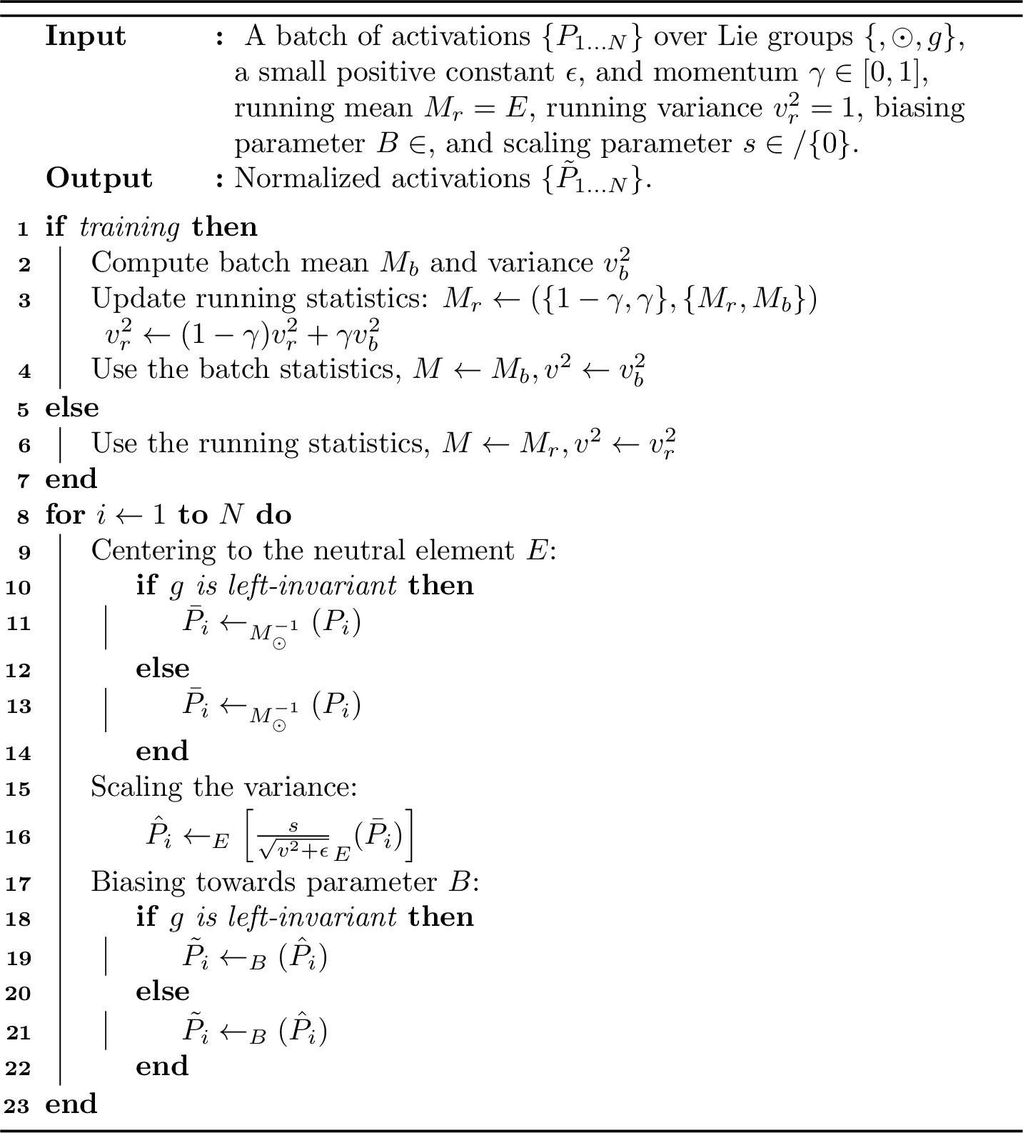
With the above ingredients, 3 presents our theoretical LieBN framework. Similar to Ioffe et al [28], we use the moving average to update the running statistics. For a bi-invariant metric, LieBN can be implemented using either left or right translation. If the Lie group is commutative, LieBN under left and right translations are equivalent. 3 summarizes the LieBN types under different conditions.
| Commutativity | Non-commutative | Commutative | ||
|---|---|---|---|---|
| Invariance | Left | Right | Bi | Left = Right = Bi |
| LieBN Types | Left | Right | Left & Right | Left = Right |
The centering and biasing in Euclidean BN correspond to the group action of \(\mathbb{R}\). From a geometric perspective, the standard Euclidean metric is invariant under this group operation. Consequently, it is not surprising that our LieBN algorithm naturally generalizes the standard Euclidean BN.
Proposition 7. The LieBN algorithm presented in 3 is equivalent to the standard Euclidean BN when \(\mathcal{M}= \mathbb{R}^{n}\), both during the training and testing phases.
Proof. The proof is presented in 15.5. ◻
5 Manifestations↩︎
This section instantiates our LieBN in 3 on nine different Lie groups, including four on the SPD manifold, one on the rotation, and four on the correlation manifold.
5.1 LieBN on SPD Manifolds↩︎
We first extend the current Lie groups on SPD manifolds by the matrix power deformation, resulting in three families of parameterized Lie groups. Then, we propose a novel right-invariant metric on the SPD manifold, the first non-trivial right-invariant metric on this manifold. Finally, we construct LieBN layers based on these Lie structures.
5.1.1 Deformed Lie Structures on SPD Manifolds↩︎
As shown in 1, there are three Lie groups on SPD manifolds, each with a left-invariant metric. These metrics include \((\alpha,\beta)\text{-AIM}\), \((\alpha,\beta)\text{-LEM}\), and LCM. For clarity, we denote the group operations w.r.t. \((\alpha,\beta)\text{-AIM}\), \((\alpha,\beta)\text{-LEM}\) and LCM as \(\odot^{\mathrm{AI}}\), \(\odot^{\mathrm{LE}}\) and \(\odot^{\mathrm{LC}}\), respectively.
Recently, Thanwerdas and Pennec [63] further extended \((\alpha,\beta)\)-AIM into three-parameter families of metrics by the pullback of matrix power function \(\mathrm{P}_\theta(\cdot)\) and scaled by \(\frac{1}{\theta^2}\), denoted as \((\theta,\alpha,\beta)\text{-AIM}\). The matrix power serves as a deformation, wherein \((\theta,\alpha,\beta)\text{-AIM}\) encompasses \((\alpha,\beta)\)-AIM with \(\theta = 1\), and becomes \((\alpha,\beta)\)-LEM as \(\theta\) approaches 0 [64]. Inspired by the deforming utility of the power function, we define the power-deformed metrics of \((\alpha,\beta)\)-LEM and LCM as the pullback metrics by \(\operatorname{P}_\theta\) and scaled by \(\frac{1}{\theta^2}\). We denote these two metrics as \((\theta,\alpha,\beta)\text{-LEM}\) and \(\theta\text{-LCM}\), respectively. We have the following results w.r.t. the deformation.
Proposition 8 (Deformation). \((\theta,\alpha,\beta)\text{-LEM}\) is equal to \((\alpha,\beta)\text{-LEM}\). \(\theta\)-LCM interpolates between \(\tilde{g}\)-LEM (\(\theta=0\)) and LCM (\(\theta=1\)). Here, given any \(P \in \mathcal{S}^{n}_{++}\) and tangent vectors \(V,W \in T_P\mathcal{S}^{n}_{++}\), \(\tilde{g}\)-LEM is defined as \[\langle V,W \rangle_P = \tilde{g}(\operatorname{log}_{*,P}(V),\operatorname{log}_{*,P}(W)),\] where \(\tilde{g}(V_1,V_2)=\frac{1}{2} \langle V_1, V_2 \rangle -\frac{1}{4} \langle \mathbb{D}(V_1), \mathbb{D}(V_2) \rangle\), \(\mathbb{D}(V_i)\) is a diagonal matrix consisting of the diagonal elements of \(V_i\), and \(\operatorname{log}_{*,P}\) is the differential map at \(P\).
Proof. The proof is presented in 15.6. ◻
As \((\theta,\alpha,\beta)\text{-LEM}\) is equal to \((\alpha,\beta)\text{-LEM}\), we focus on \((\alpha,\beta)\text{-LEM}\), \((\theta,\alpha,\beta)\text{-AIM}\), and \(\theta\text{-LCM}\) in the following. As a diffeomorphism, \(\operatorname{P}_{\theta}\) also can pull back the group operation \(\odot^{\mathrm{AI}}\) and \(\odot^{\mathrm{LC}}\), denoted as \(\odot^{\theta\text{-AI}}\) and \(\odot^{\theta\text{-LC}}\). We have the following proposition on the invariance.
Proposition 9 (Invariance). \((\theta,\alpha,\beta)\text{-AIM}\) is left-invariant w.r.t. \(\odot^{\theta\text{-AI}}\), while \(\theta\text{-LCM}\) is bi-invariant w.r.t. \(\odot^{\theta\text{-LC}}\).
Proof. The proof is presented in 15.7. ◻
5.1.2 SPD Right-invariant Metrics↩︎
AIM is left-invariant w.r.t. \(\odot^{\mathrm{AI}}\). We also can define right-invariant metric w.r.t \(\odot^{\mathrm{AI}}\) by definition [40]: \[g^{\mathrm{CRI}}_{P} (V,W) = \left\langle \operatorname{R}_{P_{\odot^{\mathrm{AI}}}^{-1}*,P} (V) , \operatorname{R}_{P_{\odot^{\mathrm{AI}}}^{-1}*,P} (W)\right\rangle_{I}\] where \(\operatorname{R}_{(\cdot)}\) denotes Lie group right translation, \(P_{\odot^{\mathrm{AI}}}^{-1}\) is the inverse of \(P\) under \(\odot^{\mathrm{AI}}\), and \(\left\langle \cdot , \cdot \right\rangle_{I}\) denotes an arbitrary inner product on \(T_I\mathcal{S}^{n}_{++}\). We set \(\left\langle \cdot, \cdot \right\rangle_{I}\) the same as the AIM at \(I\), i.e., \(\left\langle \cdot, \cdot \right\rangle^{(\alpha,\beta)}\). We call this metric the Cholesky Right Invariant Metric (CRIM), as the group operation is defined by the matrix product of Cholesky factors [3].
Theorem 10. Given any SPD matrices \(P,Q\) and tangent vector \(V \in T_P\mathcal{S}^{n}_{++}\), the Riemannian operators on \(\{\mathcal{S}^{n}_{++},g^{\mathrm{CRI}}\}\) are \[\begin{align} g^{\mathrm{CRI}}_{P}(V,V) &= \left( \left \| \left( L(L^{-1} V L^{-\top})_{\frac{1}{2}} L^{-1} \right)_{\mathrm{Sym}} \right \|^{(\alpha,\beta)} \right)^2 \\ \tag{13} \operatorname{d}(P,Q) &= \left \| \operatorname{log}\left( \widetilde{Q}^{-\frac{1}{2}} \widetilde{P} \widetilde{Q}^{-\frac{1}{2}}\right) \right \| ^{(\alpha,\beta)}, \\ \tag{14} \operatorname{Exp}_{P}(V) &= \left( \operatorname{Exp}_{\widetilde{P}}^{\mathrm{AI}} \left(-\bar{V} \right)\right)_{\odot^{\mathrm{AI}}}^{-1},\\ \tag{15} \operatorname{Log}_{P}(Q) &=-\left(L L^{\top} \left( L \widetilde{V}L^{\top} \right)_{\frac{1}{2}}^{\top} \right)_{\mathrm{Sym}}, \end{align}\] where \(L\) is the Cholesky factor of \(P=LL^\top\), \((\cdot)_{\odot^{\mathrm{AI}}}^{-1}\) is the group inverse, \(\widetilde{Q}\) and \(\widetilde{P}\) are the group inverses of \(P\) and \(Q\), \(\bar{V}=\left( \left(L^{-1} V L^{-\top}\right)_{\frac{1}{2}} L^{-1} L^{-\top} \right)_{\mathrm{Sym}}\), and \(\widetilde{V}=\operatorname{Log}^{\mathrm{AI}} _{\widetilde{P}} \left(\widetilde{Q} \right)\). Here, \(\left(X \right)_{\mathrm{Sym}}=X + X^\top, \forall X \in \mathbb{R}^{n \times n}\) denotes symmetrization, and \((\cdot)_{\frac{1}{2}}\) as its inverse map, namely \((X)_{\frac{1}{2}}=\lfloor X \rfloor + \frac{1}{2}\mathbb{X}\).
Proof. The proof is presented in 15.8. ◻
Corollary 1. CRIM is geodesically complete, and the associated geodesic connecting SPD matrices \(P\) and \(Q\) is \[\begin{align} \gamma _{(P,Q)} (t) &= \left\{ \gamma^{\mathrm{AI}}(t; \widetilde{P},\widetilde{Q}) \right\}_{\odot^{\mathrm{AI}}} ^{-1}\\ &= \left\{\widetilde{P}^{\frac{1}{2}} \left( \widetilde{P}^{-\frac{1}{2}} \widetilde{Q} \widetilde{P}^{-\frac{1}{2}} \right)^t \widetilde{P}^{\frac{1}{2}} \right\}_{\odot^{\mathrm{AI}}} ^{-1}, \end{align}\] where \(\widetilde{P}=P^{-1}_{\odot^{\mathrm{AI}}}\) and \(\widetilde{Q} = Q^{-1}_{\odot^{\mathrm{AI}}}\) are group inverses, with \(\gamma^{\mathrm{AI}}\) as the geodesic under AIM.
Proof. The proof is presented in 15.9. ◻
Similar to the discussion in 5.1.1, we define \(\theta\)-CRIM as the deformed metric of CRIM by the pullback of matrix power function \(\mathrm{P}_\theta(\cdot)\) and scaled by \(\frac{1}{\theta^2}\). As the pullback of CRIM, \(\theta\)-CRIM is right-invariant w.r.t. \(\odot^{\theta\text{-AI}}\) by definition.
Proposition 11. \(\theta\)-CRIM is right-invariant w.r.t. \(\odot^{\theta\text{-AI}}\).
5.1.3 Manifestations on SPD Manifolds↩︎
As discussed in [subsubsec:spd_param_lie_groups] [subsubsec:right_invariance], there are four families of invariant metrics on the SPD Lie groups: (1) left-invariant \((\theta,\alpha,\beta)\text{-AIM}\) w.r.t. \(\odot^{\mathrm{AI}}\); (2) bi-invariant \((\alpha,\beta)\text{-LEM}\) w.r.t. \(\odot^{\mathrm{LE}}\) and \(\theta\)-LCM w.r.t. \(\odot^{\mathrm{LC}}\); (3) right-invariant \(\theta\)-CRIM w.r.t. \(\odot^{\mathrm{AI}}\). Since all the above metrics are pullback metrics, the LieBN based on these metrics can be simplified and calculated in the co-domain. We first show a general result on LieBN under the pullback metric. We denote 3 on the Lie group \(\mathcal{M}\) as \[\operatorname{LieBN}(P_i;B,s,\epsilon,\gamma), \forall P_i \in \{P_{1 \ldots N} \in \mathcal{M}\}.\] Then we can obtain the following theorem.
Theorem 12. Given a Lie group \(\mathcal{M}_1\), a Lie group \(\mathcal{M}_2\) with an invariant metric \(g^2\), and a diffeomorphism \(f:\mathcal{M}_1 \rightarrow \mathcal{M}_2\), then \(f\) induces an invariant metric \(g^1\) on \(\mathcal{M}_1\), denoted as \(g^1=f^*g^2\). For a batch of activation \(\{P_{1 \ldots N}\}\) in \(\mathcal{M}_1\), \(\operatorname{LieBN}^1(P_i;B,s,\epsilon,\gamma)\) in \(\mathcal{M}_1\) can be calculated in \(\mathcal{M}_2\) by the following process: \[\begin{align} &\text{Mapping data into } \mathcal{M}_2: \bar{P_i} =f(P_i), \bar{B}=f(B),\\ \label{eq:liebn95pm95codomain} &\text{Performing LieBN in } \mathcal{M}_2 : \hat{P_i} = \operatorname{LieBN}^2(\bar{P_i};\bar{B},s,\epsilon,\gamma),\\ &\text{Mapping the resulting data back to } \mathcal{M}_1: \tilde{P_i} =f^{-1}(\hat{P}_i), \end{align}\tag{16}\] where \(\operatorname{LieBN}^2\) is the LieBN on \(\mathcal{M}^2\).
Proof. The proof is presented in 15.10. ◻
Given a metric \(g\) on \(\mathcal{S}^{n}_{++}\), the power-deformed metric \(\tilde{g}=\frac{1}{\theta^2}\operatorname{P}_{\theta}^*g\) is equal to \(\operatorname{P}_{\theta}^*(\frac{1}{\theta^2} g)\). 12 indicates that the LieBN under \(\tilde{g}\) can be calculated by the LieBN under \(\frac{1}{\theta^2} g\). Besides, as the Christoffel symbols remain the same under constant scaling, the LieBNs under \(\frac{1}{\theta^2} g\) and \(g\) only differ in the variance. We denote \(g^{(\alpha,\beta)\text{-AI}}\) and \(g^{(\theta,\alpha,\beta)\text{-AI}}\) as the metric tensors of \((\alpha,\beta)\text{-AIM}\) and \((\theta,\alpha,\beta)\text{-AIM}\), respectively. Based on the above discussions, the computations of the LieBN under \(g^{(\theta,\alpha,\beta)\text{-AI}}\) are reduced to the LieBN under \(\frac{1}{\theta^2}g^{(\alpha,\beta)\text{-AI}}\). Similarly, denoting \(g^{\mathrm{CRI}}\) and \(g^{\theta\text{-CRI}}\) as the metric tensors of CRIM and \(\theta\)-CRIM, then the LieBN under \(\theta\)-CRIM can be calculated by the one under \(\frac{1}{\theta^2}g^{\mathrm{CRI}}\). Furthermore, as shown by Chen et al [22], \((\alpha,\beta)\text{-LEM}\) is a pullback metric from the Euclidean space \(\mathcal{S}^{n}\) of symmetric matrices, while \(\theta\)-LCM is a pullback metric from the Euclidean space \(\mathrm{LT}^{n}\) of lower triangular matrices. As shown in 7, the LieBN in the Euclidean space \(\mathcal{S}^{n}\) or \(\mathrm{LT}^{n}\) is simplified to the standard Euclidean BN. Therefore, the LieBNs under \((\alpha,\beta)\text{-LEM}\) and \(\theta\)-LCM can be calculated by the Euclidean BN over \(\mathcal{S}^{n}\) and \(\mathrm{LT}^{n}\), respectively.
We denote the LieBN under left and right translations as LieBN-Left and LieBN-Right, respectively. Then, the LieBNs under \((\theta,\alpha,\beta)\text{-AIM}\) and \(\theta\)-CRIM correspond to LieBN-Left and LieBN-Right, respectively. As \(\odot^{\mathrm{LC}}\) and \(\odot^{\mathrm{LE}}\) are commutative, the LieBN-Left and LieBN-Right under \((\alpha,\beta)\text{-LEM}\), and \(\theta\)-LCM are equivalent. We denote \(P, Q, P_1\) and \(P_2\) as points in the codomain, i.e., \(\mathcal{S}^{n}_{++}\) with scaled CRIM for \(\theta\)-CRIM, \(\mathcal{S}^{n}_{++}\) with scaled \((\alpha,\beta)\text{-AIM}\) for \((\theta,\alpha,\beta)\text{-AIM}\), \(\mathcal{S}^{n}\) for \((\alpha,\beta)\text{-LEM}\), and \(\mathrm{LT}^{n}\) for \(\theta\)-LCM, respectively. For CRIM, we denote \(\widetilde{P}_i= (P_i)^{-1}_{\odot^{\mathrm{AI}}}\) for \(i=1,2\). We summarize all the necessary ingredients in ¿tbl:tab:ops95liebn95spd? for calculating SPD LieBN. Note that for \((\theta,\alpha,\beta)\text{-AIM}\), our scaling operation defined in 11 encompasses the scaling operation in [57] as a special case, when \((\theta,\alpha,\beta)=(1,1,0)\).
5.2 LieBN on Rotation Matrices↩︎
As the Riemannian metric on the rotation matrices is bi-invariant, there are two instantiations of LieBN on this manifold, i.e., LieBN-Left based on the left translation and LieBN-Right based on the right translation. Particularly, the scaling can be further simplified: \(\operatorname{Exp}_{I} \left( t \operatorname{Log}_{I} \left( R \right) \right) = \operatorname{exp}\left( t \operatorname{log}\left(R\right) \right)\). For the specific \(\mathrm{SO}(3)\), the matrix exp and log can be efficiently calculated without matrix decomposition [2]. ¿tbl:tab:liebn95rotations? presents the expressions of the required operators in 3.
5.3 LieBN on Full-Rank Correlation Matrices↩︎
| Metric | ECM | LECM | OLM | LSM |
|---|---|---|---|---|
| Invariance | Bi-invariance | |||
| LieBN Type | LieBN-Left = LieBN-Right | |||
| Pullback Map | \(\Theta\) | \(\log \circ \Theta\) | \(\offlog\) | \(\logscaled\) |
| Codomain | \(\{\LTone{n}, \inner{\cdot}{\cdot} \}\) | \(\{\LTzero{n}, \inner{\cdot}{\cdot} \}\) | \(\{\hol{n}, \holinner{\cdot}{\cdot} \}\) | \(\{\rzero{n}, \rzeroinner{\cdot}{\cdot} \}\) |
As discussed in 2.4, all four correlation metrics are bi-invariant, and their associated Lie groups are commutative. Consequently, LieBN-Left is identical to LieBN-Right. Moreover, all four correlation metrics are pullback metrics from simpler Euclidean space. Therefore, LieBN over the correlation can be implemented as 12: (1) map the correlation into the prototype Euclidean space, (2) apply Euclidean BN, and (3) map back to the correlation.
Optimization. Lastly, let us talk about the optimization of the correlation-valued biasing parameter \(B \in \mathcal{C}^{n}_{++}\). As shown by [3], the correlation matrix can be identified by the product of hyperbolic spaces via the Cholesky decomposition. Given \(C \in \mathcal{C}^{n}_{++}\), the \(k\)-th row of the Cholesky factor \(L=\operatorname{Chol}(C)\) is \(\left(L_{k 1}, \ldots, L_{k, k-1}, L_{k k}, 0, \ldots, 0\right)\) with \(L_{k k}>0\), which belongs to the hyperbolic space of open hemisphere \(\mathrm{HS}^{k-1} =\left\{x \in \mathbb{R}^k \mid\|x\|=1, x_k>0 \right\}\). Besides, the open hemisphere \(\mathrm{H}\mathbb{S}^{n}\) is isometric to the Poincaré ball \(\mathbb{P}^{n}=\left\{x \in \mathbb{R}^{n} \mid \|x\| < 1 \right\}\) by \(\pi _{\mathrm{H}\mathbb{S}^{n} \rightarrow \mathbb{P}^{n}} ((x^\top, x_{n+1})^\top) = \frac{x}{1+x_{n+1}}\). Therefore, each correlation can be parameterized with \(n-1\) Poincaré vectors. Each Poincaré vector can be optimized by the well-studied Riemannian optimization [65]. The above process can be expressed as \[C {\mapsto} \begin{pmatrix} 1 & 0 & \cdots & 0 \\ L_{21} & L_{22} & \cdots & 0 \\ \vdots & \vdots & \ddots & \vdots \\ L_{n1} & L_{n2} & \cdots & L_{nn} \end{pmatrix} {\mapsto} \begin{pmatrix} x_1 \in \mathbb{P}^{1} \\ \vdots \\ x_{n-1} \in \mathbb{P}^{n-1} \end{pmatrix}.\]
6 Experiments↩︎
This section validates our LieBN on nine invariant metrics across the SPD, rotation, and correlation matrices.
6.1 Experiments of LieBN on the SPD Manifold↩︎
Note that our LieBN layers are architecture-agnostic and can be applied to any existing SPD neural network. Following the previous work [9], [32], [33], we focus on two network architectures: (1) SPDNet [9] for drone recognition on the Radar dataset [32], and human action recognition on the HDM05 [66] and FPHA [67] datasets; (2) TSMNet [33] for EEG classification on the Hinss2021 dataset [68]. In the EEG application, TSMNet is endowed with SPD domain-specific momentum batch normalization (TSMNet+SPDDSMBN) [33], which is a domain adaptation version of [57]. For a fair comparison, we also implement a domain-specific momentum LieBN, referred to as DSMLieBN (detailed in 12). The backbone network architectures are represented as \(\{d_0, d_1, \ldots, d_L\}\), where the dimension of the parameter in the \(i\)-th BiMap layer (10) is \(d_i \times d_{i-1}\). As \((\alpha,\beta)\) only affects variance calculation throughout LieBN, we simply set \((\alpha,\beta)=(1,0)\) and only tune the deformation factor \(\theta\). For each family of LieBN or DSMLieBN, we report two representatives: the standard one induced from the standard metric (\(\theta=1\)), and the one induced from the deformed metric with proper \(\theta\). If the standard one is already saturated, we only report the results of the standard ones. More details on implementation, datasets, and hyperparameter \((\theta,\alpha,\beta)\) are presented in 14.1.
c|cc|*4>cc|>cc [6]*Acc & [6]*SPDNet & [6]*SPDNetBN &
& & & &
& & & AIM-(1) & LEM-(1) & LCM-(1) & CRIM-(1) & LCM-(-0.5)
& 0.98 & 1.56 & 1.62 & 1.28 & 1.11 & 1.82 & 1.43
Mean±STD & 93.25±1.10 & 94.85±0.99 & 95.47±0.90 & 94.89±1.04 & 93.52±1.07 & 94.35±0.68 & 94.80±0.71
Max & 94.4 & 96.13 & 96.27 & 96.8 & 95.2 & 95.6 & 95.73
c|c|c|*4>cc|*3>cc & [6]*SPDNet & [6]*SPDNetBN &
& & & &
& & & AIM-(1) & LEM-(1) & LCM-(1) & CRIM-(1) & AIM-(1.5) & LCM-(0.5) & CRIM-(0.5)
Fit time (s) & 0.57 & 0.97 & 1.14 & 0.87 & 0.66 & 1.37 & 1.46 & 1.01 & 1.74
Mean±STD & 59.13±0.67 & 66.72±0.52 & 67.79±0.65 & 65.05±0.63 & 66.68±0.71 & 63.25±0.88 & 68.16±0.68 & 70.84±0.92 & 65.76±0.54
Max & 60.34 & 67.66 & 68.75 & 66.05 & 68.52 & 64.94 & 69.25 & 72.27 & 66.96
c|c|c|*4>cc|*3>cc [6]*Acc & [6]*SPDNet & [6]*SPDNetBN &
& & & &
& & & AIM-(1) & LEM-(1) & LCM-(1) & CRIM-(1) & AIM-(1.5) & LCM-(0.5) & CRIM-(-0.5)
Fit time (s) & 0.32 & 0.62 & 0.8 & 0.55 & 0.39 & 0.92 & 1.03 & 0.65 & 1.21
Mean±STD & 85.59±0.72 & 89.33±0.49 & 89.70±0.51 & 86.56±0.79 & 77.64±1.00 & 84.65±1.20 & 90.39±0.66 & 86.33±0.43 & 86.40±0.57
Max & 86 & 90.17 & 90.5 & 87.83 & 79 & 86.67 & 92.17 & 87 & 87.17
Application to SPDNet: As SPDNet is the most classic SPD network, we apply our LieBN to SPDNet on the Radar, HDM05, and FPHA datasets. Additionally, we compare our method with SPDNetBN, which applies the SPDBN in 5 6 to SPDNet. Following [32], [69], we use the architectures of \(\{20,16,8\}\), \(\{93,30\}\), and \(\{63,33\}\) for the Radar, HDM05 and FPHA datasets, respectively. The 10-fold average results, including the average training time (s/epoch), are summarized in ¿tbl:tab:results95spdnet?. We have three key observations regarding the choice of metrics, deformation, and training efficiency.
The choice of metrics: The metric that yields the most effective LieBN layer differs for each dataset. Specifically, the optimal LieBN layers on these three datasets are the ones induced by AIM-(1), LCM-(0.5), and AIM-(1.5), respectively, which improves the performance of SPDNet by 2.22%, 11.71%, and 4.8%. Additionally, although the LCM-based LieBN performs worse than other LieBN variants on the Radar and FPHA datasets, it exhibits the best performance on the HDM05 dataset. These observations highlight the advantage of the generality of our LieBN framework.
The effect of deformation: Deformation patterns also vary across datasets. Firstly, the standard AIM and CRIM are already saturated on the Radar dataset. Secondly, the appropriate deformation \(\theta\) can further enhance the performance of LieBN. Notably, even though the LieBNs induced by LCM-(1) and CRIM-(1) impede the learning of SPDNet on the FPHA datasets, they can improve the performance under an appropriate deformation \(\theta\). These findings highlight the efficacy of the deforming geometry on the SPD manifold.
Efficiency: Although our LieBN involves additional computations on variance compared with SPDNetBN, our LieBN achieves comparable or even better efficiency than SPDNetBN. Particularly, the LieBN induced by standard LEM or LCM exhibits better efficiency than SPDNetBN. Even with deformation, the LCM-based LieBN is still comparable with SPDNetBN in terms of efficiency. This phenomenon could be attributed to the fast and simple computation of LCM and LEM.
| Method | Fit Time | Mean±STD | |
|---|---|---|---|
| SPDDSMBN | 0.16 | 54.12±9.87 | |
| DSMLieBN | AIM-(1) | 0.16 | 55.10±7.61 |
| LEM-(1) | 0.13 | 54.95±10.09 | |
| LCM-(1) | 0.10 | 51.54±6.88 | |
| CRIM-(1) | 0.29 | 51.86±9.21 | |
| LCM-(0.5) | 0.15 | 53.11±5.65 | |
| Method | Fit Time | Mean±STD | |
|---|---|---|---|
| SPDDSMBN | 7.74 | 50.10±8.08 | |
| DSMLieBN | AIM-(1) | 6.94 | 50.04±8.01 |
| LEM-(1) | 4.71 | 50.95±6.40 | |
| LCM-(1) | 3.59 | 51.86±4.53 | |
| CRIM-(1) | 16.35 | 50.71±8.1 | |
| CRIM-(1.5) | 19.51 | 51.34±5.82 | |
| AIM-(-0.5) | 8.71 | 53.97±8.78 | |
Application to EEG classification: We apply our method to TSMNet under two scenarios, inter-session and inter-subject. Following [33], we adopt the architecture of \(\{40,20\}\). Compared to SPDDSMBN, DSMLieBN-AIM obtains the highest average scores of 55.10% and 53.97% in these two scenarios, outperforming SPDDSMBN by 0.98% and 3.87%, respectively. In the inter-subject scenario, the advantage of the efficiency of our LieBN over SPDDSMBN is more obvious. Specifically, both the LEM- and LCM-based DSMLieBN achieve similar or better performance compared to SPDDSMBN, while requiring considerably less training time. For example, DSMLieBN-LCM-(1) achieves better results with only half the training time of SPDDSMBN on inter-subject tasks. Interestingly, under the standard AIM, the sole difference between SPDDSMBN and our DSMLieBN is the way of centering and biasing. SPDDSMBN applies the matrix inverse square root and matrix square root to fulfill centering and biasing, while AIM-induced LieBN uses more efficient Cholesky decomposition. As such, the DSMLieBN induced by the standard AIM is more efficient than SPDDSMBN, particularly on the inter-subject task. On the other hand, the CRIM-based LieBN shows less efficiency, due to the relatively complex Riemannian computation of this metric.
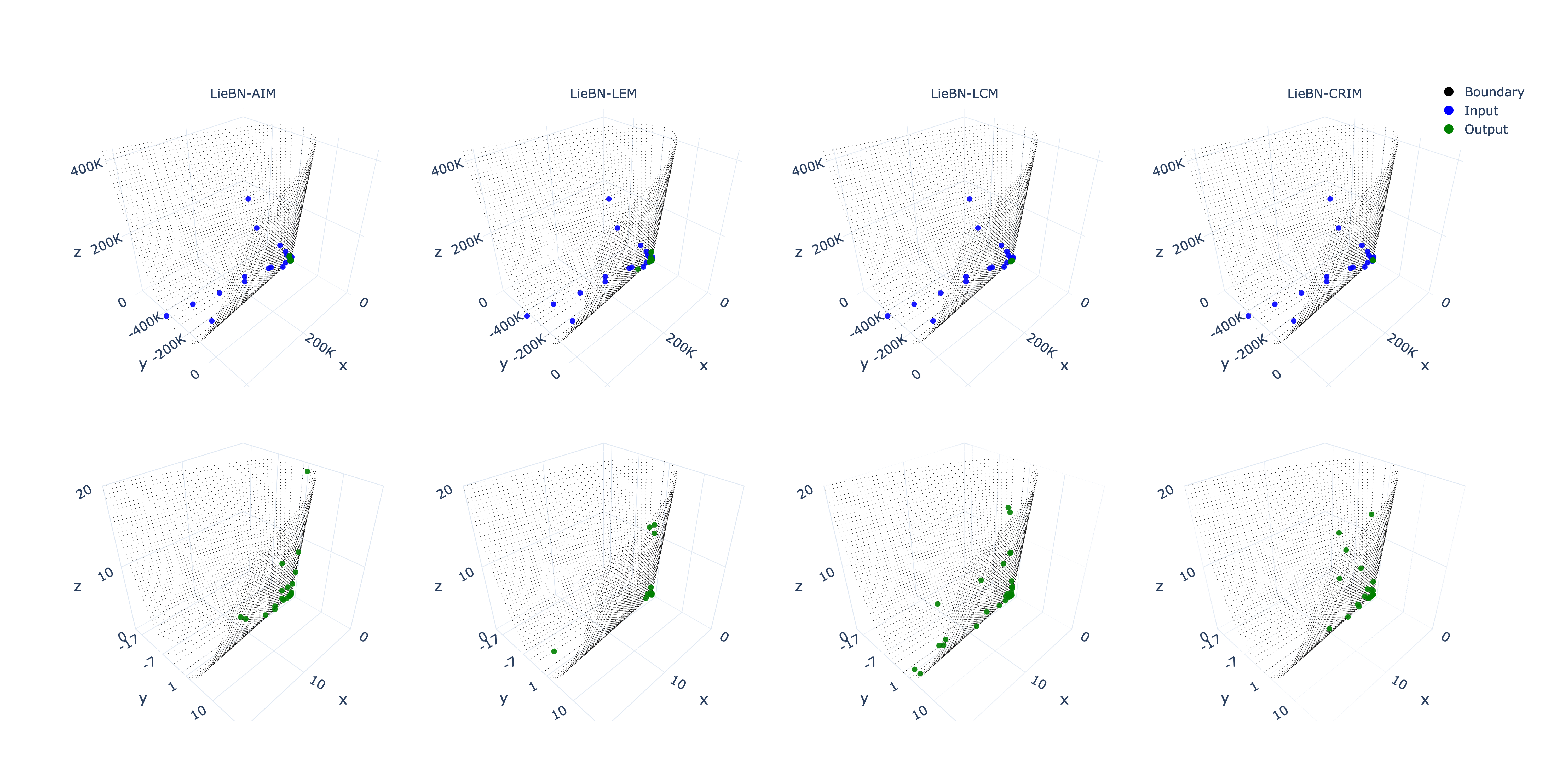
Visualization: We randomly select 50 samples and visualize the input and output of LieBN on the HDM05 dataset. Using Riemannian t-SNE [70], we map the \(30 \times 30\) SPD matrices to \(2 \times 2\) low-dimensional representations. As shown in 4, LieBN effectively normalizes the data distribution. Specifically, the input t-SNE embeddings are largely scattered and their elements can reach up to 400K, whereas those of the output embeddings are mostly constrained within 20.
6.2 Experiments of LieBN on Rotation Matrices↩︎
This subsection implements our LieBN on the special orthogonal groups, i.e., \(\mathrm{SO}(n)\), also known as rotation matrices. As the Riemannian metric on \(\mathrm{SO}(n)\) is bi-invariant, there are two instantiations of our LieBN on this group: LieBN-Left based on the left translation and LieBN-Right based on the right translation. We apply our LieBN to the classic LieNet backbone [10], where the latent space is the special orthogonal group. Following [10], we use three action recognition datasets, the G3D [71], HDM05 [66], and NTU60 [72] datasets. We denote the LieNet models with our LieBN-Left and LieBN-Right as LieNetLieBN-Left and LieNetLieBN-Right, respectively. More implementation details are presented in 14.2.
| Method | G3D | HDM05 | NTU60 | |||
|---|---|---|---|---|---|---|
| 2-7 | Mean±STD | Max | Mean±STD | Max | 2Blocks | 3Blocks |
| LieNet | 87.91±0.90 | 89.73 | 76.92±1.27 | 79.11 | 62.4 | 60.91 |
| LieNetLieBN-Left | 88.88±1.62 | 90.67 | 78.89±1.07 | 80.88 | 63.51 | 62.62 |
| LieNetLieBN-Right | 88.12±1.12 | 90.3 | 79.39±1.13 | 80.67 | 63.6 | 62.72 |
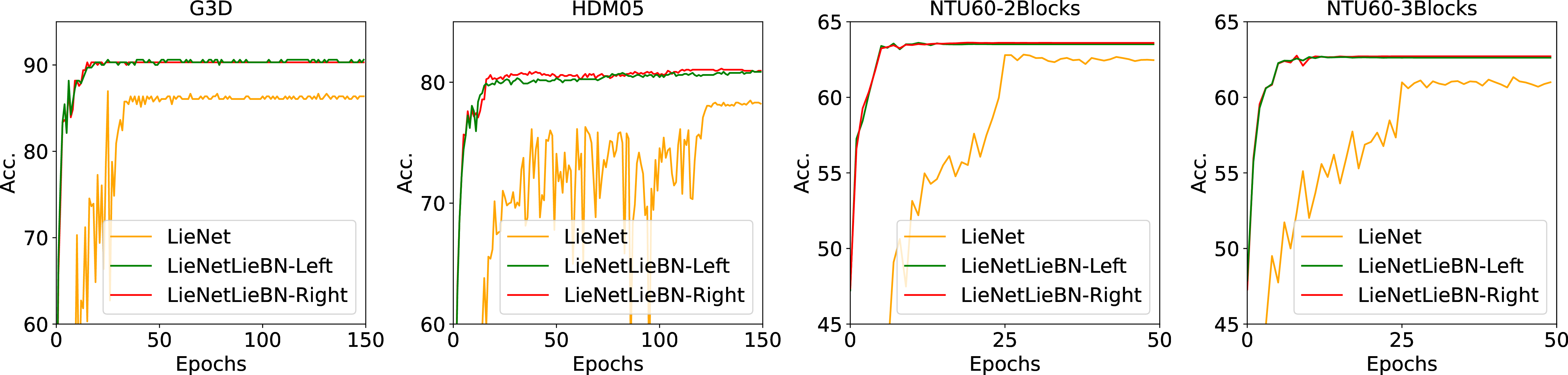
Results: We conduct 10-fold experiments on the G3D and HDM05 datasets under the suggested 3Blocks5 and 2Blocks architectures, respectively. On the NTU60 dataset, we validate LieBN under the 2Blocks and 3Blocks settings. The results are presented in 5. Due to differences in software, our reimplemented LieNet (by PyTorch) performs slightly differently from the results reported in [10] (by Matlab). However, we still observe a clear improvement when applying our LieBN to the vanilla LieNet backbone. Additionally, LieBN-Right performs slightly better than LieBN-Left. Although the effects of left and right translations on the sample statistics under the bi-invariant metric are identical, their transformations on each sample differ, as illustrated in 1. This difference could slightly affect the network performance. The specific optimal choice of left or right translations depends on the dataset’s characteristics.
Training Dynamics: 5 presents the test accuracy curve. We have the following additional observations, which can be attributed to the mitigated covariate shift by our LieBN, as our LieBN can effectively normalize the sample statistics. Accelerated convergence: LieBN significantly accelerates the convergence of LieNet. Specifically, on the NTU60 dataset—the largest dataset involved—LieNet with LieBN converges by the 5th epoch, whereas the vanilla LieNet does not converge until the 25th epoch. A similar phenomenon can also be observed on the HDM05 dataset. Stabler performance: LieBN enhances the stability of network training. Especially on the HDM05 and G3D datasets, the initial training fluctuations are greatly mitigated by our LieBN.
6.3 Experiments of LieBN on Correlation Matrices↩︎
As no neural networks are specifically designed for the correlation manifold and correlation matrices are still SPD, we apply our correlation LieBN (LieBN-Cor) to SPD networks. Our experiments focus on the SPDNet backbone using the FPHA and HDM05 datasets. LieBN-Cor is applied before the final classification layer. Specifically, SPD features are first activated by the power function, then mapped into correlation matrices via \(\operatorname{Cor}(\cdot)\), and finally processed by LieBN-Cor. More details can be found in 14.3.
c|c|*4>cc [4]*Dataset & [4]*SPDNet &
& & ECM & LECM & OLM & LSM
HDM05 & 59.13±0.67 & 65.37 ± 1.07 & 61.35 ± 0.34 & 60.33 ± 0.12 & 60.00 ± 0.27
FPHA & 85.59±0.72 & 87.20 ± 0.12 & 87.03 ± 0.32 & 86.80 ± 0.12 & 86.77 ± 0.29
Result: The 5-fold average results are presented in ¿tbl:tab:results95liebn95cor?. Although LieBN-Cor is not specifically designed for SPD networks, it still improves SPDNet’s performance, demonstrating its effectiveness. Among the four invariant metrics, ECM achieves the best performance. While LieBN-SPD outperforms LieBN-Cor when applied to SPDNet—an expected result since SPDNet is tailored for SPD matrices—this does not undermine the validity of LieBN-Cor. The consistent improvement over vanilla SPDNet highlights the potential of applying LieBN-Cor to correlation manifolds.
| ECM | LECM | OLM | LSM | |
|---|---|---|---|---|
| Trivialization | 63.17 ± 1.32 | 58.84 ± 0.51 | 59.84 ± 0.45 | 53.22 ± 1.62 |
| Riemannian | 65.37 ± 1.07 | 61.35 ± 0.34 | 60.33 ± 0.12 | 60.00 ± 0.27 |
Ablations: As discussed in 5.3, the correlation-valued biasing parameter \(B \in \mathcal{C}^{n}_{++}\) is optimized via Riemannian optimization over multiple Poincaré vectors. Alternatively, trivialization tricks [73] can be employed. Specifically, 12 suggests that we can instead set \(\bar{B} = f(B) \in V\) as the parameter, where \(f\) is the isometry and \(V\) is the prototype space for ECM, LECM, OLM, and LSM, respectively. 6 presents the 5-fold comparison, demonstrating the superiority of our Poincaré parameterization.
7 Conclusions↩︎
This paper presents a novel LieBN framework for batch normalization over Lie groups, leveraging natural Lie-group-invariant metrics. Compared to prior approaches, LieBN provides a principled method to normalize both sample and population statistics. Empirically, we generalize three existing Lie group structures on the SPD manifold and introduce the first non-trivial right-invariant SPD metric. By employing these parameterized invariant metrics, we instantiate our framework on the SPD manifold. Furthermore, we implement LieBN on rotation matrices using a bi-invariant metric and on the correlation manifold using four bi-invariant metrics. Extensive experiments across different manifolds validate the effectiveness of our LieBN.
Acknowledgments↩︎
Acknowledgment↩︎
This work was supported by the MUR PNRR project FAIR (PE00000013) funded by the NextGenerationEU, and the EU Horizon project ELIAS (No. 101120237). The authors are also grateful for the HPC resources from the ISCRA project.
Ziheng Chen received the B.A. degree in logistics management from Shandong University, Jinan, China, and M.S. degree in computer science and technology from Jiangnan University, Wuxi, China. He is currently working toward the Ph.D. degree with the Multimedia and Human Understanding Group (MHUG), University of Trento, Trento, Italy. His research interests are geometric deep learning and matrix & vector manifolds.
Yue Song received the B.Sc. cum laude from KU Leuven, Belgium and the joint M.Sc. summa cum laude from the University of Trento, Italy and KTH Royal Institute of Technology, Sweden, and the Ph.D. summa cum laude from the Multimedia and Human Understanding Group (MHUG) at the University of Trento, Italy. Currently, he is a post-doctoral research associate at Caltech. His research interests are structured representation learning.
Rui Wang received the M.S. degree in computer science from Jiangnan University, Wuxi, China, in 2018, and the Ph.D. degree in pattern recognition and intelligent system from Jiangnan University, Wuxi, China, in 2023. He is currently a Lecturer with the School of Artificial Intelligence and Computer Science, Jiangnan University. His research topics include Riemannian manifold learning, metric learning, and deep learning.
Xiao-Jun Wu received the B.Sc. degree in mathematics from Nanjing Normal University, Nanjing, China, in 1991. He received the M.S. degree and the Ph.D. degree in pattern recognition and intelligent systems from Nanjing University of Science and Technology, Nanjing, China, in 1996 and 2002, respectively. He is a distinguished professor in the School of Artificial Intelligence and Computer Science, Jiangnan University. He is a fellow of IAPR and AAIA.
Nicu Sebe is Professor with the University of Trento, Italy, leading the research in the areas of multimedia information retrieval and human behavior understanding. He was the General Co-Chair of ACM Multimedia 2013, and the Program Chair of ACM Multimedia 2007 and 2011, ECCV 2016, ICCV 2017 and ICPR 2020. He is a fellow of IAPR.
to 2cm
LieBN: Batch Normalization over Lie Groups (Supplement)
Ziheng Chen, Yue Song, Rui Wang, Xiao-Jun Wu, and Nicu Sebe
8 Notations↩︎
For better clarity, we summarize all the notations used in this paper in 7.
| Notation | Explanation |
|---|---|
| \(\{\calM, \odot, g \}\) or abbreviated as \(\calM\) | Lie group with a group operation \(\odot\) and an invariant metric \(g\) |
| \(\gleft\) and \(\gright\) | Left-invariant and right-invariant metrics |
| \(P_\odot ^{-1}\) | Group inverse of \(P \in \calM\) |
| \(T_P\calM\) | Tangent space at \(P \in \calM\) |
| \(g_p(\cdot ,\cdot)\) or \(\langle \cdot, \cdot \rangle_P\) | Riemannian metric at \(P \in \calM\) |
| \(\| \cdot \|_P\) | Norm induced by \(\langle \cdot, \cdot \rangle_P\) on \(T_P\calM\) |
| \(\dist(\cdot,\cdot)\) | Geodesic distance |
| \(\fm\) and \(\wfm\) | Fréchet mean and weighted Fréchet mean |
| \(\rieexp_P\) and \(\rielog_P\) | Riemannian exponentiation and logarithm at \(P\) |
| \(\gamma _{(P,Q)}(t)\) | Geodesic connecting \(P\) and \(Q\) |
| \(\pt{P}{Q}\) | Riemannian parallel transportation along the geodesic connecting \(P\) and \(Q\) |
| \(\ltrans_P\) and \(\rtrans_P\) | Lie group left and right translation by \(P \in \calM\) |
| \(f_{*,P}\) | Differential map of the smooth map \(f\) at \(P \in \calM\) |
| \(f^*g\) | Pullback metric by \(f\) from \(g\) |
| \(\bbR{n \times n}\) | Euclidean space of \(n \times n\) real matrices |
| \(\spd{n}\) | SPD manifold of \(n \times n\) SPD matrices |
| \(\sym{n}\) | Euclidean space of \(n \times n\) symmetric matrices |
| \(\trilspace{n}\) | Euclidean space of \(n \times n\) lower triangular matrices |
| \(\so{n}\) | Lie group of \(n \times n\) rotation matrices |
| \(\soLieAlgebra{n}\) | Euclidean space of \(n \times n\) skew-symmetric matrices |
| \(\langle \cdot, \cdot \rangle\) and \(\| \cdot \|_\rmF\) | Standard Frobenius inner product and the induced norm |
| \(\langle \cdot, \cdot \rangle^{\alphabeta}\) and \(\| \cdot \|^{\alphabeta}\) | \(\orth{n}\)-invariant Euclidean inner product and the induced norm |
| \(\bfst\) | \(\bfst = \{(\alpha,\beta) \in \mathbb{R}^2 \mid \min (\alpha, \alpha+n \beta)>0\}\) |
| \(\gbiparamai\), \(\gtriparamAI\), \(\gcri\) and \(\gdefcri\) | Riemannian metric tensor of \(\biparamAIM\), \(\triparamAIM\), CRIM, and \(\theta\)-CRIM |
| \(\odotai\), \(\odotle\), and \(\odotlc\) | Group operations w.r.t. AIM, LEM, and LCM |
| \(\symmetrize{\cdot}\) | \(\symmetrize{X}=X + X^\top, \forall X \in \bbR{n \times n}\) |
| \((\cdot)_{\frac{1}{2}}\) | \((X)_{\frac{1}{2}}=\lfloor X \rfloor + \frac{1}{2}\bbD(X), \forall X \in \bbR{n \times n}\) |
| \(\calN(M,\sigma^2)\) | Riemannian Gaussian distribution |
| \(\mlog\) and \(\mexp\) | Matrix logarithm and exponentiation |
| \(\chol\) | Cholesky decomposition |
| \(\dlog\) | Diagonal element-wise logarithm |
| \(\clog\) | \(\dlog \circ \chol\) |
| \(\lfloor \cdot \rfloor\) | Strictly lower triangular part of a square matrix |
| \(\pow_\theta(\cdot)\) or \((\cdot)^{\theta}\) | Matrix power function |
| \(\bbD(\cdot)\) | Returning a diagonal matrix with diagonal elements from a square matrix |
| \(\diag(\cdot)\) | Returns a diagonal matrix from an input vector |
| \(\hol{n}\) and \(\rzero{n}\) | Subspace of \(\sym{n}\) with null diagonals and null row sum |
| \(\rone{n}\) | Manifold of \(n \times n\) SPD matrices with unit row sum. |
| \(\cor{n}\) | Manifold of \(n \times n\) full-rank correlation matrices |
| \(\LTone{n}\) and \(\LTzero{n}\) | Euclidean subspaces of \(\trilspace{n}\) with unit diagonals and null diagonals |
| \(\chospace{n}\) | Cholesky manifold of \(n \times n\) lower triangular matrices with positive diagonals |
| \(\circledast\) | Hadamard product |
| \(\coropt\) | \(\coropt: \Sigma \in \spd{n} \longmapsto \bbD(\Sigma)^{-\nicefrac{1}{2}} \Sigma \bbD(\Sigma)^{-\nicefrac{1}{2}} \in \cor{n}\) |
| \(\Theta\) | \(\Theta : C \in \cor{n} \longmapsto \bbD(\chol(C))^{-1} \chol(C) \in \LTone{n}\) |
| \(\off\) | Returns a matrix in \(\hol{n}\) consisting of off-diagonal elements |
| \(\offlog \& \offexp\) | Off-log and its inverse |
| \(\logscaled \& \expscaled\) | Log-scaled and its inverse |
| \(I\) or \(I_n\) & \(\bfzero\) | Identity matrix & zero matrix |
| \(\holinner{\cdot}{\cdot}\) and \(\rzeroinner{\cdot}{\cdot}\) | Permutation-invariant inner products over \(\hol{n}\) and \(\rzero{n}\) |
9 Riemannian Structures on the Involved Matrix Manifolds↩︎
9.1 Existence and Uniqueness of the Weighted Fréchet Mean↩︎
Let \((\mathcal{M}, g)\) be an orientable complete Riemannian manifold equipped with a Riemannian metric \(g\). The induced distance is denoted as \(\operatorname{d}(\cdot,\cdot)\). We denote the supremum of the sectional curvatures of \(\mathcal{M}\) by \(\Delta\). We recover the theorem on the existence and uniqueness of the Weighted Fréchet Mean (WFM) [46]. We acknowledge that Chakraborty et al [14] has also provided a summary of the following discussions.
Definition 5 (Geodesic Ball). Let \(P \in \mathcal{M}\) and \(r > 0\). Then \(B_r(P) = \{Q \in \mathcal{M}\mid d(P, Q) < r\}\) is the open geodesic ball at \(P\) of radius \(r\).
Definition 6 (Injectivity Radius [54]). The local injectivity radius at \(P \in \mathcal{M}\), \(r_{\text{inj}}(P)\), is the largest radius \(r\) for which \(\operatorname{Exp}_P : T_P \mathcal{M}\supset B_r(0) \to \mathcal{M}\) is a diffeomorphism onto its image. The injectivity radius of \(\mathcal{M}\) is defined as \(r_{\text{inj}}(\mathcal{M}) = \inf_{P \in \mathcal{M}} \{r_{\text{inj}}(P)\}\).
Within the local injectivity radius, the exponential map is invertible and we call the inverse map as Riemannian logarithmic map, \(\operatorname{Log}_{P} : B_{r_{\text{inj}}(P)} (P) \rightarrow B _{r_{\text{inj}}(P)}(0) \subset T _P \mathcal{M}\).
Definition 7 (Regular Geodesic Ball [74]). An open geodesic ball \(B_r(P)\) is a regular geodesic ball if \(r < r_{\text{inj}}(P)\) and \(r < \pi/(2 \sqrt{\Delta})\), where \(1 / \sqrt{\Delta}\) is interpreted as \(\infty\) for \(\Delta \leq 0\).
If \(P, Q\) in a regular geodesic ball \(B_r (P)\), there exists a unique geodesic \(\gamma _{(P,Q)} :[0,1] \rightarrow B_r(P)\) with \(\gamma(0)=P\) and \(\gamma(1)=Q\) [74].
Definition 8 (Strong Convexity [75]). A subset \(U \subset \mathcal{M}\) is strongly convex if for all \(P, Q \in U\), there exists a unique length-minimizing geodesic segment between \(P\) and \(Q\), and the geodesic segment lies entirely in \(U\).
Definition 9 (Convexity Radius [76]). The local convexity radius at \(P \in \mathcal{M}\), \(r_{\text{cvx}}(P)\), is defined as \[r_{\text{cvx}}(P) = \sup \{r \le r_{\text{inj}}(P) \mid B_r(P) \text{ is strongly convex}\}.\] The convexity radius of \(\mathcal{M}\) is defined as \(r_{\text{cvx}}(\mathcal{M}) = \inf_{P \in \mathcal{M}} \{r_{\text{cvx}}(P)\}\).
Theorem 13 (Existence and Uniqueness of WFM [46]). The WFM exists and is unique inside a geodesic ball of radius \(r_{\text{cvx}}(\mathcal{M})\).
In the main paper, we always assume the involved \(\operatorname{Exp}\), \(\operatorname{Log}\), and WFM are well-defined.
9.2 Symmetric Matrix Functions↩︎
This subsection reviews the eigenvalue function over symmetric matrices. For more in-depth discussions, please refer to [77] or [78].
We denote \(\mathcal{S}^{n}\) as the Euclidean space of \(n \times n\) real symmetric matrices, and \(\mathcal{S}^{n}_{++}\) as the SPD manifold of \(n \times n\) SPD matrices. Let \(\mathring{I}\) be an open interval of \(\mathbb{R}\) and \(f: \mathring{I} \rightarrow \mathbb{R}\) be a smooth function. The smooth map induced by \(f\) for any symmetric matrix \(S\) with all eigenvalues in \(\mathring{I}\) is defined as \[f: S \longmapsto U f(\Sigma) U^\top \in \mathcal{S}^{n}, \text{ with } S=U \Sigma U^\top \text{ as the eigendecomposition.}\] Its differential is known as the Daleckĭi-Kreĭn formula: \[\begin{align} \tag{17} f_{*,S} (V) &=U\left(L \circledast \left(U^{\top} V U\right)\right) U^{\top}, \quad \forall V \in \mathcal{S}^{n}, \\ \tag{18} L_{i,j}&= \begin{cases} \frac{f(\sigma_i)-f(\sigma_j)}{\sigma_i-\sigma_j}, & \text{ if } \sigma_i \neq \sigma_j \\ f^{\prime}(\delta_i), & \text{ otherwise } \end{cases} \end{align}\] where \(L\) is called the Loewner matrix with the \((i,j)\)-th element defined as 18 , and \(\odot\) denotes the Hadamard product. Two special cases are the matrix logarithm: \(\log: \mathcal{S}^{n}_{++} \rightarrow \mathcal{S}^{n}\) and its inverse, the matrix exponentiation \(\exp: \mathcal{S}^{n} \rightarrow \mathcal{S}^{n}_{++}\).
9.3 SPD Geometries↩︎
8 summarizes the Lie groups and invariant metric on the SPD manifold with the following notations. Let \(P, Q \in \mathcal{S}^{n}_{++}\) be SPD matrices and \(V, W \in T_P\mathcal{S}^{n}_{++}\) be tangent vectors. We denote the matrix logarithm, exponentiation, and Cholesky decomposition by \(\operatorname{log}(\cdot)\), \(\operatorname{exp}(\cdot)\), and \(\operatorname{Chol}(\cdot)\), respectively. The differentials at \(P\) are \(\operatorname{log}_{*,P}\) and \(\operatorname{Chol}_{*,P}\). The Cholesky factors of \(P\) and \(Q\) are denoted as \(L=\operatorname{Chol}(P)\) and \(K=\operatorname{Chol}(Q)\). The corresponding tangent vectors are \(X = \operatorname{Chol}_{*,P} (V)\) and \(Y = \operatorname{Chol}_{*,P} (W)\) for LCM. \(\mathbb{K}\), \(\mathbb{L}\), \(\mathbb{X}\), and \(\mathbb{Y}\) are diagonal matrices with diagonal elements from \(K\), \(L\), \(X\), and \(Y\), respectively. \(\lfloor \cdot \rfloor\) is the strictly lower part of a square matrix. The norms induced by \(\langle \cdot, \cdot \rangle^{(\alpha,\beta)}\) and the standard Frobenius norm (induced by the standard inner product \(\left\langle \cdot, \cdot\right \rangle\)) by \(\| \cdot \|^{(\alpha,\beta)}\) and \(\| \cdot \|_\mathrm{F}\), respectively.
| Metric | \(\biparamLEM\) | \(\biparamAIM\) | LCM |
|---|---|---|---|
| \(Q \odot P\) | \(\mexp(\mlog(P)+\mlog(Q))\) | \(KPK^\top\) | \(\chol^{-1}(\lfloor L + K \rfloor + \bbK \bbL)\) |
| \(g_P(V,W)\) | \(\langle \mlog_{*,P} (V), \mlog_{*,P} (W) \rangle^{\alphabeta}\) | \(\langle P^{-1}V, W P^{-1} \rangle^{\alphabeta}\) | \(\langle \lfloor X \rfloor, \lfloor Y \rfloor \rangle + \langle \bbX \bbL^{-1}, \bbY \bbL^{-1} \rangle\) |
| \(\dist(P,Q)\) | \(\left \|\mlog(P)-\mlog(Q) \right\|^{\alphabeta}\) | \(\left \|\mlog \left(Q^{-\frac{1}{2}}PQ^{-\frac{1}{2}} \right) \right\|^{\alphabeta}\) | \(\left \| \clog (P) - \clog (Q) \right \|_\rmF\) |
| \(\fm (\{P_i\})\) | \(\mexp \left( \frac{1}{n} \sum_i \mlog{P_i} \right)\) | Karcher Flow | \(\clog^{-1} \left( \frac{1}{n} \sum_i \clog(P_i) \right)\) |
| \(\rielog_P Q\) | \((\mlog_{*,P})^{-1} \left[ \mlog(Q) - \mlog(P) \right]\) | \(P^{\frac{1}{2}} \mlog \left(P^{ -\frac{1}{2}} Q P^{-\frac{1}{2}}\right) P^{\frac{1}{2}}\) | \((\chol^{-1})_{*, L} \left[ \lfloor K\rfloor-\lfloor L\rfloor+\bbL \dlog (\bbL^{-1} \bbK) \right]\) |
| \(\rieexp _P V\) | \(\mexp \left( \mlog(P) + \mlog _{*,P} (V) \right)\) | \(P^{\frac{1}{2}} \mexp \left(P^{ -\frac{1}{2}} V P^{-\frac{1}{2}}\right) P^{\frac{1}{2}}\) | \(\chol^{-1} \left( \lfloor L \rfloor + \lfloor X \rfloor + \bbL \exp \left( \bbX \bbL^{-1} \right) \right)\) |
| \(\gamma _{(P,Q)} (t)\) | \(\mexp \left[ \mlog(P) + t\left(\mlog(Q) - \mlog(P)\right) \right]\) | \(P^{\frac{1}{2}} \left(P^{ -\frac{1}{2}} Q P^{-\frac{1}{2}}\right)^{t} P^{\frac{1}{2}}\) | \(\chol^{-1} \left\{ \lfloor L \rfloor + t(\lfloor K \rfloor- \lfloor L \rfloor) + \frac{\bbK^t}{\bbL^{t-1}} \right\}\) |
| Invariance | Bi-invariance | Left-invariance | Bi-invariance |
| References | [36], [51], [69] | [3], [50], [51] | [21], [37], [69] |
9.4 Rotation Geometries↩︎
Given \(R, S \in \mathrm{SO}(n)\), and tangent vectors \(A_1, A_2 \in T_R \mathrm{SO}(n)\), 9 summarizes all the associated operators on \(\mathrm{SO}(n)\) under the invariant metric, where \(\langle \cdot, \cdot \rangle\) denotes the standard Frobenius inner product.
| Operators | \(R \odot S\) | \(g_R (A_1,A_2)\) | \(\dist(R,S)\) | \(\rielog_R S\) | \(\rieexp_R(A)\) | \(\gamma_{(R,S)}(t)\) | FM | Invariance |
|---|---|---|---|---|---|---|---|---|
| Expression | \(RS\) | \(\langle A_1, A_2 \rangle\) | \(\left\|\mlog \left(R^{\top} S\right)\right\|_\rmF\) | \(R \mlog(R^\top S)\) | \(R\mexp(R^\top A)\) | \(R \mexp (t \mlog(R^\top S))\) | [54] | Bi-invariance |
9.5 Correlation Geometries↩︎
| Metric | Prototype space | Diffeomorphisms | Properties |
|---|---|---|---|
| ECM [3] | \(\LTone{n} = \LTzero{n} + I_n\) | ||
| \(\Theta^{-1} = \coropt \circ \chol^{-1} : \LTone{n} \longrightarrow \cor{n}\) | Bi-invariance | ||
| LECM [3] | \(\LTzero{n}\) | ||
| \((\log \circ \Theta)^{-1} = \coropt \circ \chol^{-1} \circ \exp: \LTzero{n} \longrightarrow \cor{n}\) | Bi-invariance | ||
| OLM [39] | \(\hol{n}\) | ||
| \((\offlog) ^{-1} = \offexp: H \in \hol{n} \longmapsto \exp ( \dplus(H) + H ) \in \cor{n}\) | |||
| Permutation-invariance | |||
| LSM [39] | \(\rzero{n}\) | ||
| \((\logscaled)^{-1} = \expscaled: R \in \rzero{n} \longmapsto \coropt(\exp(R)) \in \cor{n}\) | |||
| Permutation-invariance |
The involved four geometries in 2.4 on the correlation matrices can be classified into two classes: (1) non-permutation-invariant metrics, including ECM and LECM; and (2) permutation-invariant metrics, including OLM and LSM. 10 summarizes the diffeomorphisms and prototype spaces discussed in 2.4.
9.5.1 None-permutation-invariant Metrics↩︎
The non-permutation-invariant metrics [3], namely ECM and LECM, are defined by isometries: \[\begin{align} \text{ECM: }& \mathcal{C}^{n}_{++} \xrightleftharpoons[\Theta^{-1} = \operatorname{Cor}\circ \operatorname{Chol}^{-1}]{\Theta} \mathrm{LT}_1^{n} = I_n + \mathrm{LT}_0^{n}, \\ \text{LECM: }& \mathcal{C}^{n}_{++} \xrightleftharpoons[(\log \circ \Theta)^{-1} = \operatorname{Cor}\circ \operatorname{Chol}^{-1} \circ \exp]{\log \circ \Theta} \mathrm{LT}_0^{n}, \end{align}\]
ECM and LECM. For any \(C \in \mathcal{C}^{n}_{++}\), \(V \in T_C \mathcal{C}^{n}_{++} \cong \mathrm{Hol}^{n}\), \(K \in \mathrm{LT}_1^{n}\) and \(X, \xi \in \mathrm{LT}_0^{n}\), the involved maps and their differentials in ECM and LECM are \[\begin{align} \Theta(C) &= \mathbb{D}(L)^{-1} L, \\ \Theta^{-1} (K) &= \mathbb{D}\left(K K^{\top}\right)^{-\frac{1}{2}} K K^{\top} \mathbb{D}\left(K K^{\top}\right)^{-\frac{1}{2}}, \\ \tag{19} \log (K) &=\sum_{k=1}^{n-1} \frac{(-1)^{k-1}}{k}\left(K-I_n\right)^k, \\ \tag{20} \exp (\xi) &=\sum_{k=0}^{n-1} \frac{1}{k!} \xi^k, \\ \tag{21} \Theta_{*,C}(V) &= \Theta(C) \left(L^{-1} V L^{-\top}\right)_{\frac{1}{2}} -\frac{1}{2} \mathbb{D}\left(L^{-1} V L^{-\top}\right) \Theta(C),\\ \left(\Theta_{*,C} \right)^{-1}(\xi) &= \left( L \xi^{\top}-C \mathbb{D}\left(L \xi^{\top}\right)\right) \mathbb{D}(L) +\mathbb{D}(L)\left(\xi L^{\top}-\mathbb{D}\left(L \xi^{\top}\right) C \right), \\ \tag{22} \log_{*,K} (\xi) &= \sum_{k=1}^{n-1} \frac{(-1)^{k-1}}{k}\left[\left(K-I_n\right)^{k-1} \xi +\left(K-I_n\right)^{k-2} \xi\left(K-I_n\right)+\cdots+\xi\left(K-I_n\right)^{k-1}\right], \\ \exp_{*, X} (\xi) &= \sum_{k=1}^{n-1} \frac{1}{k!}\left(X^{k-1} \xi+X^{k-2} \xi X+\cdots+\xi X^{k-1}\right), \\ \tag{23} (\log \circ \Theta)_{*,C} (V) &= \log_{*, \Theta(C)} \left( \Theta_{*,C}(V) \right),\\ \tag{24} \operatorname{Chol}_{*,C} (V) &= L \left(L^{-1} V L^{-\top}\right)_{\frac{1}{2}}, \\ (\operatorname{Chol}_{*,C})^{-1} (Z) &= L Z^\top + Z L^\top, \quad \forall Z \in T_L \mathrm{LT}_{++}^{n} \cong \mathrm{LT}^{n}. \end{align}\] where \(L\) is the Cholesky factor of \(C\), \(I_n\) is the \(n \times n\) identity matrix and \(\mathrm{LT}_{++}^{n}\) is the Cholesky manifold of \(n \times n\) Cholesky matrices. Due to the nilpotency of \(\mathrm{LT}_0^{n}\), the matrix logarithm over \(\mathrm{LT}_1^{n}\) and exponentiation over \(\mathrm{LT}_0^{n}\) are free from eigendecomposition. With the above equations, 11 summarizes the Riemannian operators under ECM and LECM.
| Operation | ECM | LECM |
|---|---|---|
| \(g_{C}(V,W)\) | \(\inner{\Theta_{*, C}(V)}{\Theta_{*, C}(W)}\) | \(\inner{(\log \circ \Theta)_{*, C}(V)}{(\log \circ \Theta)_{*, C}(W)}\) |
| \(\rieexp_C(V)\) | \(\Theta^{-1}\left(\Theta\left(C\right) + \Theta_{*, C} \left( V\right)\right)\) | \((\log \circ \Theta)^{-1}\left(\log \circ \Theta\left(C\right) + (\log \circ \Theta)_{*, C} \left( V \right) \right)\) |
| \(\rielog_C(C')\) | \(\Theta^{-1}_{{*, \Theta(C)}}\left(\Theta\left(C'\right) - \Theta\left(C\right)\right)\) | \((\log \circ \Theta)^{-1}_{{*, \log \circ \Theta(C)}}\left(\log \circ \Theta\left(C'\right) - \log \circ \Theta\left(C\right)\right)\) |
| \(\gamma(t;C,C')\) | \(\Theta^{-1}\left(\left(1 - t\right)\Theta\left(C\right) + t\Theta\left(C'\right)\right)\) | \((\log \circ \Theta)^{-1}\left(\left(1 - t\right)\log \circ \Theta\left(C\right) + t\log \circ \Theta\left(C'\right)\right)\) |
| \(\dist(C, C')\) | \(\fnorm{ \Theta\left(C\right) - \Theta\left(C'\right) }\) | \(\fnorm{ \log \circ \Theta\left(C\right) - \log \circ \Theta\left(C'\right) }\) |
| Fréchet mean | \(\Theta^{-1}\left(\frac{1}{k} \sum_{i=1}^{k} \Theta\left(C_i\right)\right)\) | \((\log \circ \Theta)^{-1}\left(\frac{1}{k} \sum_{i=1}^{k} \log \circ \Theta\left(C_i\right)\right)\) |
| Curvature | \(0\) | \(0\) |
| \(\pt{C}{C'} (V)\) | \(\left(\Theta_{*, C'} \right)^{-1}\left(\Theta_{*, C} \left(V\right)\right)\) | \(\left((\log \circ \Theta)_{*, C'}\right)^{-1}\left((\log \circ \Theta)_{*, C} \left(V\right)\right)\) |
9.5.2 Permutation-invariant Metrics↩︎
Let \(\mathfrak{S}^{n}\) be the group of permutation matrices \(P_\sigma=\left[\delta_{i, \sigma(j)}\right]_{1 \leqslant i, j \leqslant n}\) by permutation \(\sigma\), and \(\mathcal{D}^{\pm}(n)=\left\{\operatorname{diag}\left( \left(\varepsilon_1, \ldots, \varepsilon_n \right) \right), \varepsilon \in\{-1,1\}^n\right\}\) be the group of diagonal matrices with coefficients in \(\{-1,1\}\). [39] showed that the biggest congruence action on full-rank correlation matrices is the action of signed permutation matrices: \[\star:(A, C) \in \mathfrak{S}^{\pm}(n) \times \mathcal{C}^{n}_{++} \longmapsto A C A^{\top} \in \mathcal{C}^{n}_{++},\] with \(\mathfrak{S}^{\pm}(n)=\mathcal{D}^{\pm}(n) \mathfrak{S}^{n}\). Based on this finding, [39] proposed two permutation-invariant metrics, namely OLM and LSM, by pulling back permutation-invariant inner products via the following permutation-equivariant diffeomorphisms: \[\begin{align} \mathcal{C}^{n}_{++} &\xrightleftharpoons[\operatorname{Exp}^{\circ}]{\operatorname{Log}^{\circ}=\mathrm{Off}\circ \log} \mathrm{Hol}^{n},\\ \mathcal{C}^{n}_{++} &\xrightleftharpoons[\operatorname{Exp}^{\star}=\operatorname{Cor}\circ \exp]{\operatorname{Log}^{\star}} \mathrm{Row}_0^{n}, \\ \operatorname{Exp}^{\circ}: \mathrm{Hol}^{n} \ni H &\longmapsto \exp(\mathcal{D}^+(H) + H), \\ \operatorname{Log}^{\star}: \mathcal{C}^{n}_{++} \ni C &\longmapsto \log ( \mathcal{D}^\star(C) C \mathcal{D}^\star(C)) \in \mathrm{Row}_0^{n}. \end{align}\] where \(\log(\cdot)\) and \(\exp(\cdot)\) are symmetric matrix logarithm and exponentiation. The involved \(\mathcal{D}^+\) and \(\mathcal{D}^\star\) can be formally expressed as \(\mathcal{D}^+: \mathrm{Hol}^{n} \rightarrow \mathbb{D}^{n}\) and \(\mathcal{D}^\star: \mathcal{C}^{n}_{++} \rightarrow \mathbb{D}_{+}^{n}\), where \(\mathbb{D}^{n}\) denotes the Euclidean space of \(n \times n\) diagonal matrices, and \(\mathbb{D}_{+}^{n}\) is the submanifold of \(\mathbb{D}^{n}\), consisting of positive diagonal matrices.
The differentials of \(\operatorname{Log}^{\circ}\) and \(\operatorname{Log}^{\star}\) and their inverses can be calculated by the differential of symmetric matrix logarithm and exponentiation [39]. Given \(C \in \mathcal{C}^{n}_{++}\), tangent vector \(V \in T_C\mathcal{C}^{n}_{++} \cong \mathrm{Hol}^{n}\), \(H, W \in \mathrm{Hol}^{n}\), and \(S = H+\mathcal{D}^+(H) = U \Delta U^{\top}\), the differential of \(\operatorname{Log}^{\circ}\) and its inverse \(\operatorname{Exp}^{\circ}\) are \[\begin{align} \tag{25} \operatorname{Log}^{\circ}_{*,C} (V) &=\mathrm{Off}\left(\log_{*,C} (V)\right),\\ \operatorname{Exp}^{\circ}_{*,H}(W) & = \exp_{*, S} \left(W+\mathcal{D}^+_{*,H}(W)\right), \\ \tag{26} \mathcal{D}^+_{*,H} (W) & =-\operatorname{diag}\left(\left(H^0\right)^{-1} \mathbb{D}\left( \exp_{*, S} (W)\right) \boldsymbol{1}\right), \\ \mathcal{S}^{n}_{++} \ni H_{i l}^0 &= \sum_{j, k} P_{i j} P_{i k} P_{l j} P_{l k} L_{j,k}, \end{align}\] where \(L\) is the Loewner matrix of \(\exp_{*, S}\), and \(\boldsymbol{1}\) is the vector of all 1 entities. Here, \(\log_{*}\) and \(\exp_{*}\) can be calculated using the Daleckii-Krein formula of the symmetric matrix, while \(\operatorname{diag}(\cdot): \mathbb{R}^{n} \rightarrow \mathbb{D}^{n}\) returns a diagonal matrix from an input vector. Further denoting \(X, Y \in \operatorname{Row}_0(n)\) and \(\Sigma=\mathcal{D}^\star(C) C \mathcal{D}^\star(C)\), the differentials of \(\operatorname{Log}^{\star}\) and its inverse \(\operatorname{Exp}^{\star}\) are \[\begin{align} \label{app:eq:diff95logscaled} \operatorname{Log}^{\star}_{*,C}(V) &=\log_{*,\Sigma} \left(\Delta V \Delta+\frac{1}{2}\left(V^0 \Sigma+\Sigma V^0\right)\right),\\ \operatorname{Exp}^{\star}_{*,X}(Y) &=\Delta^{-1}\left[\exp_{*,X} (Y)-\frac{1}{2}\left(\Delta^{-2} \mathbb{D}\left(\exp_{*,X} (Y)\right) \Sigma+\Sigma \mathbb{D}\left(\exp_{*,X} (Y)\right) \Delta^{-2}\right)\right] \Delta^{-1} \end{align}\tag{27}\] with \(\Delta=\mathbb{D}(\Sigma)^{1 / 2}\) and \(V^0=-2 \operatorname{diag}\left(\left(I_n+\Sigma\right)^{-1} \Delta V \Delta \boldsymbol{1}\right)\).
As both \(\operatorname{Log}^{\star}_{*}\) and \(\operatorname{Log}^{\circ}_{*}\) are permutation-equivariant [39], permutation-invariant metrics over the correlation manifold can be induced by permutation-invariant inner products over \(\mathrm{Hol}^{n}\) and \(\mathrm{Row}_0^{n}\), respectively. The following two theorems review such inner products.
| Operation | OLM | LSM |
|---|---|---|
| \(g_{C}(V,W)\) | \(\holinner{\offlog_{*, C}(V)}{\offlog_{*, C}(W)}\) | \(\rzeroinner{\logscaled_{*, C}(V)}{\logscaled_{*, C}(W)}\) |
| \(\rieexp_C(V)\) | \(\offexp\left(\offlog\left(C\right) + \offlog_{*, C} \left( V\right)\right)\) | \(\expscaled\left(\logscaled\left(C\right) + \logscaled_{*, C} \left( V \right) \right)\) |
| \(\rielog_C(C')\) | \(\offexp_{{*, \offlog(C)}}\left(\offlog\left(C'\right) - \offlog\left(C\right)\right)\) | \(\expscaled_{{*, \logscaled(C)}}\left(\logscaled\left(C'\right) - \logscaled\left(C\right)\right)\) |
| \(\gamma(t;C,C')\) | \(\offexp\left(\left(1 - t\right)\offlog\left(C\right) + t\offlog\left(C'\right)\right)\) | \(\expscaled\left(\left(1 - t\right)\logscaled\left(C\right) + t\logscaled\left(C'\right)\right)\) |
| \(\dist(C, C')\) | \(\holnorm{ \offlog\left(C\right) - \offlog\left(C'\right) }\) | \(\rzeronorm{ \logscaled\left(C\right) - \logscaled\left(C'\right) }\) |
| Fréchet mean | \(\offexp\left(\frac{1}{k} \sum_{i=1}^{k} \offlog\left(C_i\right)\right)\) | \(\expscaled\left(\frac{1}{k} \sum_{i=1}^{k} \logscaled\left(C_i\right)\right)\) |
| Curvature | \(0\) | \(0\) |
| \(\pt{C}{C'} (V)\) | \(\left(\offlog_{*, C'} \right)^{-1}\left(\offlog_{*, C} \left(V\right)\right)\) | \(\left(\logscaled_{*, C'}\right)^{-1}\left(\logscaled_{*, C} \left(V\right)\right)\) |
| Invariance | ||
| Permutation-invariance | ||
| Singed-permutation-invariance \((\beta=\gamma=0)\) | ||
| Permutation-invariance |
Theorem 14 (Permutation-Invariant Inner Products on \(\mathrm{Hol}^{n}\) [79]). Supposing \(n \geq 4\), permutation-invariant inner products on \(\mathrm{Hol}^{n}\) are: \[\left \langle X_1, X_2 \right \rangle^{(\alpha,\beta,\gamma)} = \alpha \operatorname{tr}( X_1 X_2) +\beta \operatorname{Sum}\left(X_1 X_2\right)+\gamma \operatorname{Sum}(X_1) \operatorname{Sum}(X_2), \quad \forall X_1,X_2 \in \mathrm{Hol}^{n},\] with \(\alpha > 0\), \(2\alpha + (n - 2)\beta > 0\), and \(\alpha + (n - 1)(\beta + n\gamma) > 0\). For \(n = 3\), permutation-invariant inner products have the same form with \(\alpha = 0\): \[\left \langle X_1, X_2 \right \rangle^{(\alpha,\beta,\gamma)} = \beta \operatorname{Sum}(X_1 X_2) + \gamma \operatorname{Sum}(X_1)\operatorname{Sum}(X_2), \quad \text{with } \beta > 0 \text{ and } \beta + 3\gamma > 0.\] For \(n = 2\), they have the same form with \(\alpha = \beta = 0\): \[\left \langle X_1, X_2 \right \rangle^{(\alpha,\beta,\gamma)} = \gamma \operatorname{Sum}(X_1)\operatorname{Sum}(X_2), \quad \text{with } \gamma > 0.\]
Theorem 15 (Permutation-Invariant Inner Products on \(\mathrm{Row}_0^{n}\) [39]). For \(n \geq 4\), permutation-invariant inner products on \(\mathrm{Row}_0^{n}\) are \[\left \langle Y_1, Y_2 \right \rangle^{(\alpha,\delta,\zeta)} = \alpha \operatorname{tr}(Y_1 Y_2) + \delta \operatorname{tr}(\mathbb{D}(Y_1)\mathbb{D}(Y_2)) + \zeta \operatorname{tr}(Y_1)\operatorname{tr}(Y_2), \quad \forall Y_1,Y_2 \in \mathrm{Row}_0^{n},\] with \(\alpha > 0\), \(n\alpha + (n-2)\delta > 0\), and \(n\alpha + (n-1)(\delta + n\zeta) > 0\). For \(n = 3\), the permutation-invariant inner products have the same form with \(\alpha = 0\). For \(n = 2\), they have the same form with \(\alpha = \delta = 0\).
As shown by [79], the OLM is further signed-permutation invariant under \(\beta=\gamma=0\), reduced to the scaled canonical Euclidean inner product: \[\left \langle V, W \right \rangle^{(\alpha,\beta,\gamma)} = \alpha \left\langle V, W\right \rangle, \quad \forall V,W \in \mathrm{Hol}^{n}.\] In the main paper, we assume that \(\left \langle \cdot, \cdot \right \rangle^{(\alpha,\beta,\gamma)}\) and \(\left \langle \cdot, \cdot \right \rangle^{(\alpha,\delta,\zeta)}\) are the canonical Euclidean inner product. 12 summarizes the Riemannian structures of OLM and LSM.
Remark 16. \(\mathcal{D}^+\) is also well-defined over \(\mathcal{S}^{n}\), a surjective map \(\mathcal{D}^+: \mathcal{S}^{n} \rightarrow \mathbb{D}^{n}\). In this way, \(\operatorname{Exp}^{\circ}: \mathcal{S}^{n} \rightarrow \mathcal{C}^{n}_{++}\) is no longer bijective [39]. Similarly, \(\mathcal{D}^\star\) is well defined over \(\mathcal{S}^{n}_{++}\), a surjective map \(\mathcal{D}^\star: \mathcal{S}^{n}_{++} \rightarrow \mathbb{D}_{+}^{n}\). Consequently, \(\operatorname{Log}^{\star}: \mathcal{S}^{n}_{++} \rightarrow \mathrm{Row}_0^{n}\) is no longer bijective [39].
10 Basic Layers in SPDNet and TSMNet↩︎
SPDNet [9] is the most classic SPD neural network. SPDNet mimics the conventional densely connected feedforward network, consisting of three basic building blocks \[\begin{align} &\text{BiMap layer: } S^{k} = W^{k} S^{k-1} W^{k\top}, \text{ with } W^k \text{ semi-orthogonal,}\\ &\text{ReEig layer: } S^{k}=U^{k-1} \max (\Sigma^{k-1}, \epsilon I_{n}) U^{k-1 \top}, \text{ with } S^{k-1}=U^{k-1} \Sigma^{k-1} U^{k-1 \top},\\ &\text{LogEig layer: } S^{k}=\log(S^{k-1}). \end{align}\] where \(\max(\cdot)\) is element-wise maximization. BiMap and ReEig mimic transformation and non-linear activation, while LogEig maps SPD matrices into the tangent space at the identity matrix for classification.
TSMNet [33] can be illustrate as \(f_{tc} \rightarrow f_{sc} \rightarrow f_{BiMap} \rightarrow f_{ReEig} \rightarrow f_{LogEig}\), where \(f_{tc}\) and \(f_{sc}\) denote temporal and spatial convolution, respectively.
11 Statistical Results of Scaling in LieBN↩︎
In this section, we will show the effect of our scaling (11 ) on the population. We will see that while the resulting population variance is generally agnostic, it becomes analytic under certain circumstances, such as SPD manifolds under LEM or LCM. As a result, 11 can normalize and transform the latent Gaussian distribution.
To simplify, let \(\phi_s(P) = \operatorname{Exp}_{E} \left[ s \operatorname{Log}_{E}(P) \right]\). Similar to the main paper, \(\mathcal{M}\) denotes a Lie group with a left-invariant metric. First, we present a lemma on the resulting P.D.F. of a random point transformed by \(\phi_s\).
Lemma 1. Given a random point \(X\) distributed over \(\mathcal{M}\) with P.D.F. \(p_X\), the P.D.F of \(Y=\phi_s(X)\) is given by: \[p_Y(Q)=\Delta p_{X}(\phi_s^{(-1)}(Q) ).\] where \(\Delta=\frac{|\phi^{-1}_{s*}|}{\left|L_{\phi_s^{-1}(Q)\odot Q^{-1}*} \right|}\). Here \(| \cdot |\) denotes the determinant, and \(\phi^{-1}_{s*}\) and \(L_{\phi_s^{-1}(Q)\odot Q^{-1}*}\) are the differentials.
Proof. For the sake of simplicity, we will denote \(\phi_s\) as \(\phi\) throughout this proof. The volume element w.r.t. a left-invariant metric is the Haar measure [80]: \[\operatorname{d}_L \mathcal{M}(P)= \frac{d P}{|L_{P*,E}|},\] where \(|L_{P*,E}|\) is the determinant6 of the differential of \(L_P\) at the neutral element \(E\). Then we have \[\begin{align} \operatorname{d}_L \mathcal{M}(\phi^{-1}(Q)) &= \frac{\operatorname{d}\phi^{-1}(Q)}{|L_{\phi^{-1}(Q)*,E}|}\\ &= |(L_{\phi^{-1}(Q) \odot Q^{-1}} \circ L_{Q})_{*,E} |^{-1} |\phi^{-1}_{*}| \operatorname{d}Q\\ &= \frac{|\phi^{-1}_{*}|}{|L_{\phi^{-1}(Q)\odot Q^{-1}*} |} \operatorname{d}_{L}\mathcal{M}(Q)\\ &= \Delta \operatorname{d}_{L}\mathcal{M}(Q). \end{align}\]
The probability of \(Q=\phi(P)\) in a set \(\mathcal{Y}\subset \mathcal{M}\) is \[\begin{align} F( \phi(P) \in \mathcal{Y}) &=F( P \in \phi^{-1} (\mathcal{Y}) )\\ &=\int_{\phi^{-1} (\mathcal{Y})} p_{X}(P) \cdot d_L \mathcal{M}(P)\\ &=\int_{\mathcal{Y}} p_{X}(\phi^{(-1)}(Q) ) d_L \mathcal{M}(\phi^{(-1)}(Q))\\ &=\int_{\mathcal{Y}} \Delta p_{X}(\phi^{(-1)}(Q) ) d_L \mathcal{M}(Q). \end{align}\] Therefore, the density of \(Y=\phi(X)\) is \[p_Y(Q)=\Delta p_{X}(\phi^{(-1)}(Q)).\] ◻
The above lemma implies that when \(\Delta\) is a constant, \(Y\) also follows a Gaussian distribution.
Corollary 2. Following the notations in 1, if \(\Delta=c\) is a constant and \(X \sim \mathcal{N}(E,\sigma^2)\), then \(Y\) also follows a Gaussian distribution, i.e.\(Y \sim \mathcal{N}(E,s^2\sigma^2)\)
Proof. \[\begin{align} p_{Y}(Q) &= ck(\sigma) \exp \left(-\frac{\operatorname{d}(\phi_s^{-1}(Q), E)^2}{2 \sigma^2}\right)\\ &= k'(\delta) \exp \left(-\frac{\operatorname{d}(\operatorname{Exp}_E \frac{1}{s} \operatorname{Log}_E(Q), E)^2}{2 \sigma^2}\right)\\ &= k'(\delta) \exp \left(-\frac{\| \operatorname{Log}_E(Q) \|_E^2}{2 s^2\sigma^2}\right)\\ &= k'(\delta) \exp \left(-\frac{\operatorname{d}(Q,E)}{2 s^2\sigma^2}\right), \end{align}\] where \(\| \cdot \|_E\) is the norm of the tangent space at the neutral element \(E\). ◻
2 implies that when \(\Delta=c\), \(\phi_s\) can scale the population variance and further transform the Gaussian distribution. Simple computations show that in the standard Euclidean space \(\mathbb{R}^{n}\), \(\Delta=\frac{1}{s}\). Therefore, it is natural to expect that the pullback of \(\mathbb{R}^{n}\) also enjoys constant \(\Delta\).
Proposition 17. Consider an \(n\)-dimensional Lie group \(\mathcal{M}\) pulled back from the standard Euclidean space \(\mathbb{R}^{n}\) by the diffeomorphism \(\psi:\mathcal{M}\rightarrow \mathbb{R}^{n}\). In other words, the group operations and Riemannian metric on \(\mathcal{M}\) are defined by \(\psi\) from \(\mathbb{R}^{n}\). Then \(\Delta\) remains constant on \(\mathcal{M}\).
Proof. To simplify notation, we denote \(\phi_s\) as \(\phi\). Under the given assumption, the group addition and Riemannian metric on \(\mathcal{M}\) are defined as follows: \[\begin{align} \forall P,Q \in \mathcal{M}, P \odot Q &= \psi^{-1}(\psi(P)+\psi(Q))\\ g&=\psi^{*}g^{\mathrm{E}}, \end{align}\] where \(g^{\mathrm{E}}\) is the standard Euclidean metric. Therefore, \(\phi\) can be simplified as \[\begin{align} \phi(P) &=\operatorname{Exp}_{E} \left [ s \operatorname{Log}_{E}(P) \right]\\ &=\psi^{-1} \left( \tilde{\operatorname{Exp}}_{0} \left[\psi_{*,E} \left(s\psi^{-1}_{*,0} \tilde{\operatorname{Log}}_{0}\psi(P) \right)\right] \right)\\ &= \psi^{-1}(s\psi(P)), \end{align}\] where \(\tilde{\operatorname{Exp}}\) and \(\tilde{\operatorname{Log}}\) are the Riemannian exponential and logarithmic maps in \(\mathbb{R}^{n}\), which are reduced to vector addition and subtraction, respectively. Therefore, the inverse of \(\phi\) is \[\label{eq:phi95delta95simplified} \phi^{-1}(P) = \psi^{-1}\left(\frac{1}{s}\psi(P)\right).\tag{28}\] Besides, \(L_{\phi^{-1}(Q)\odot Q^{-1}}\) can also be further simplified: \[\label{eq:lt95delta95simplified} L_{\phi^{-1}(Q)\odot Q^{-1}}(P) = \psi^{-1}\left(\frac{1}{s}\psi(Q) - \psi(Q) + \psi(P)\right)\tag{29}\] The differentials of 28 29 at \(Q\) are \[\begin{align} \phi^{-1}_{*,Q}&=\frac{1}{s} \psi^{-1}_{*,\frac{1}{s}\psi(Q)} \circ \psi_{*,Q},\\ L_{\phi^{-1}(Q)\odot Q^{-1}*,Q}&= \psi^{-1}_{*,\frac{1}{s}\psi(Q)} \circ \psi_{*,Q}. \end{align}\] Therefore, \(\Delta=\frac{1}{s}\) for all \(Q \in \mathcal{M}\). ◻
By 17, we can directly obtain the following corollary.
Corollary 3. Given a Lie group \(\mathcal{M}\) pulled back from the Euclidean space, and a random point \(X \sim \mathcal{N}(E,\sigma^2)\) over \(\mathcal{M}\), \(Y=\phi_s(X) \sim \mathcal{N}(E,s^2\sigma^2)\)
In machine learning, several Lie groups are derived by the pullback from the standard Euclidean space. As shown by Chen et al [22], \((\alpha,\beta)\text{-LEM}\) and \(\theta\text{-LCM}\) are pullback metrics from the Euclidean metric. Therefore, for the Lie groups of SPD manifolds w.r.t. \((\alpha,\beta)\text{-LEM}\) and \(\theta\text{-LCM}\), 11 can transform the Gaussian distribution. Specifically, given a random point \(X \sim \mathcal{N}(M,\sigma^2)\), 10 11 12 transform the Gaussian distribution as: \[\label{eq:liebn95gaussian95lem95lcm} \mathcal{N}(M,\sigma^2) \rightarrow \mathcal{N}(E,\sigma^2) \rightarrow \mathcal{N}(E, s^2) \rightarrow \mathcal{N}(B, s^2),\tag{30}\] where \(M\) and \(\sigma\) are employed to normalize \(X\), and \(\epsilon\) in 11 is omitted. The above process exactly mirrors the transformation of Gaussian distributions within the framework of standard BN [28].
Remark 18. A similar result to our 3 was also presented in [34]. However, in his proof, the author did not account for the Haar measure and only considered the P.D.F., casting doubt on the validity of their results. Additionally, their discussion is limited to matrix Lie groups, specifically under the distance \(\operatorname{d}(P,Q)= \| \operatorname{log}(P^{-1}Q)\|_{\mathrm{F}}\). In contrast, we rectify their proof and consider general Lie groups.
12 Domain-specific Momentum LieBN for EEG Classification↩︎
Kobler et al [33] proposed SPD domain-specific momentum batch normalization (SPDDSMBN) as a domain adaptation approach for EEG classification. SPDDSMBN, based on 8 , performed normalization of mean and variance on SPD manifolds under the specific AIM. Additionally, SPDDSMBN utilized separate momentums for updating training and testing running statistics, inspired by the work of [81]. Following [33], we also present a momentum LieBN (MLieBN) in [alg:mliebn]. Here \(\gamma\) is fixed and \(\gamma_{train}\) is defined as \[\gamma_{train}=1-\rho^{\frac{1}{K-1} \max (K-k, 0)}+\rho, \;\text{where}\;\rho=\frac{1}{domains\_per\_batch}\]
Furthermore, in line with [33], we adopt multi-channel mechanisms for domain-specific MLieBN (DSMLieBN), where each domain has its own MLieBN layer. Similar to [33], we set the biasing parameter equal to the neutral element, and the scaling factor is shared across all domains. We denote [alg:mliebn] as \(\operatorname{MLieBN}(P_j | M, s, \epsilon, \gamma,\gamma_{train} )\). Then our DSMLieBN follows \[\operatorname{DSMLieBN}(P_j,i) =\operatorname{MLieBN}_i(P_j | E, s, \epsilon, \gamma,\gamma_{train} ), \forall P_j \in \{P_{1 \ldots N}\},\] where \(i\) is the index of the domain. We follow the official code of SPDDSMBN7 to implement our DSMLieBN. In a word, the only difference between DSMLieBN and SPDDSMBN is the different way of normalization.
Analogous to 12, computations for DSMLieBN under pullback metrics can also be performed by mapping, calculating, and then remapping.
13 Backpropagation of Matrix Functions↩︎
Our implementation of LieBN on SPD and correlation manifolds involves several matrix functions. Thus, we employ matrix backpropagation (BP) [82] for gradient computation. These matrix operations can be divided into Cholesky decomposition and the functions based on Eigendecomposition.
The differentiation of the Cholesky decomposition can be found in [83] or [37]. Besides, our homemade BP of the Cholesky decomposition yields a similar gradient to the one generated by autograd of torch.linalg.cholesky.
Therefore, during the experiments, we use torch.linalg.cholesky.
The second type of matrix functions is based on Eigendecomposition, such as matrix exponential, logarithm, and power. Although torch [84] supports autograd of Eigendecomposition, it requires the computation of \(\frac{1}{\delta_i-\delta_j}\) [82], where \(\delta_i\) and \(\delta_j\) denote eigenvalues. This might trigger numerical instability when \(\delta_i\) approximates \(\delta_j\). Following [32], we use the Daleckĭi-Kreĭn formula [78] to calculate the BP of Eigen-based matrix functions. In detail, for a matrix function defined as \(X = f(S) = U f(\Sigma) U^\top\), with \(S = U \Sigma U^\top\) as the eigendecomposition of an SPD matrix, its BP is expressed as \[\begin{align} \label{eq:gradient95eigen95function} \nabla_{S} L &= U[K \odot(U^{T}(\nabla_{X} L) U)] U^{T}. \end{align}\tag{31}\] where \(\nabla_{X} L\) is the Euclidean gradient of the loss function \(L\) w.r.t. \(X\). Matrix \(K\) is defined as \[\label{eq:lorenz} K_{i j}= \begin{cases}\frac{f\left(\sigma_{i}\right)-f\left(\sigma_{j}\right)}{\sigma_{i}-\sigma_{j}} & \text{ if } \sigma_{i} \neq \sigma_{j} \\ f^{\prime}\left(\sigma_{i}\right) & \text{ otherwise }\end{cases}\tag{32}\] where \(\Sigma=\operatorname{diag}(\sigma_1,\sigma_2,\cdots,\sigma_d\)). 32 demonstrates the numerical stability of Daleckĭi-Kreĭn formula.
14 Experimental Details and Additional Discussions↩︎
14.1 Experimental Details and Additional Discussion on the SPD Manifold↩︎
14.1.1 Datasets and Preprocessing↩︎
The Radar dataset [32] contains 3,000 synthetic radar signals. Following the protocol in [32], each signal is split into windows of length 20, resulting in 3,000 covariance matrices of \(20 \times 20\) equally distributed in 3 classes.
The HDM05 dataset [66] consists of 2,273 skeleton-based motion capture sequences executed by different actors. Each frame consists of 3D coordinates of 31 joints, allowing the representation of each sequence as a \(93 \times 93\) covariance matrix. In line with [32], we trim the dataset to 2086 instances scattered throughout 117 classes by removing some under-represented clips.
The FPHA [67] includes 1,175 skeleton-based first-person hand gesture videos of 45 different categories with 600 clips for training and 575 for testing. Following [85], we represent each sequence as a \(63 \times 63\) covariance matrix.
The Hinss2021 dataset [68] is a recently released competition dataset containing EEG signals for mental workload estimation. The dataset is employed for two tasks, inter-session and inter-subject, which are treated as domain adaptation problems. Geometry-aware methods [1], [33] have demonstrated promising performance in EEG classification. We follow [33] for data preprocessing. In detail, the python package MOABB [86] and MNE [87] are used to preprocess the datasets. The applied steps include resampling the EEG signals to 250/256 Hz, applying temporal filters to extract oscillatory EEG activity in the 4 to 36 Hz range, extracting short segments ( \(\leq 3\)s) associated with a class label, and finally obtaining \(40 \times 40\) SPD covariance matrices.
14.1.2 Implementation details↩︎
We use the official code of SPDNetBN8 [32] and TSMNet9 [33] to implement our experiments on the SPDNet and TSMNet backbones. For the SPDNet architecture, we compare our LieBN with SPDNetBN [32], which applies the SPDBN (5 6 ) to SPDNet. Similar to SPDNetBN, we apply our LieBN after each transformation layer (BiMap layer in 10). In the EEG application, one of the state-of-the-art methods is TSMNet with SPD domain-specific momentum batch normalization (TSMNet+SPDDSMBN) [33], which is a domain adaptation version of [57]. For a fair comparison, we also implement a domain-specific momentum LieBN, referred to as DSMLieBN (detailed in 12). Following [33], we apply our DSMLieBN before the LogEig layer (detailed in 10) in TSMNet. We use the standard cross-entropy loss and optimize the parameters with the Riemannian AMSGrad optimizer [65]. The network architectures are represented as \(\{d_0, d_1, \ldots, d_L\}\), where the dimension of the parameter in the \(i\)-th BiMap layer is \(d_i \times d_{i-1}\). The experiments are conducted with a learning rate of \(5e^{-3}\), batch size of 30, and training epoch of 200 on the Radar, HDM05, and FPHA datasets. For the Hinss2021 dataset, following [33], we use a learning rate of \(1e^{-3}\) with a weight decay of \(1e^{-4}\), a batch size of 50, and a training epoch of 50.
In line with the previous work [32], [33], we use accuracy as the scoring metric for the Radar, HDM05, and FPHA datasets, and balanced accuracy (i.e., the average recall across classes) for the Hinss2021 dataset. Ten-fold experiments on the Radar, HDM05, and FPHA datasets are carried out with randomized initialization and split (split is officially fixed for the FPHA dataset), while on the Hinss2021 dataset, models are fit and evaluated with a randomized leave 5% of the sessions (inter-session) or subjects (inter-subject) out cross-validation scheme.
14.1.3 Candidate Values of Hyper-parameters↩︎
We implement the SPD LieBN and DSMLieBN induced by four standard invariant metrics, namely AIM, LEM, LCM, and CRIM, along with their deformed metrics. Therefore, our method has a maximum of three hyper-parameters, i.e., \((\theta,\alpha,\beta)\). As \((\alpha,\beta)\) only affects variance calculation in the LieBN framework, we set \((\alpha,\beta)=(1,0)\) and only tune the deformation factor \(\theta\) from the candidate values of \(\pm 0.5\), \(\pm 1\), and \(\pm 1.5\). We denote [Baseline]+[BN_Type]+[Metric]-[\(\theta\)] as the baseline endowed with a specific LieBN, such as SPDNet+LieBN-AIM-(1) and TSMNet+DSMLieBN-LCM-(1).
14.1.4 Empirical Insights on the Hyper-parameters↩︎
Our SPD LieBN has at most three types of hyper-parameters: Riemannian metric, deformation factor \(\theta\), and \(\mathrm{O}({n})\)-invariance parameters \((\alpha,\beta)\). The general order of importance should be Riemannian metric \(>\) \(\theta\) \(>\) \((\alpha,\beta)\).
The most significant parameter is the choice of Riemannian metric, as all the geometric properties are sourced from a metric. A safe choice would start with AIM, and then decide whether to explore other metrics further. The most important reason is the property of affine invariance of AIM, which is a natural characteristic of covariance matrices. In our experiments, the LieBN-AIM generally achieves the best performance. However, AIM is not always the best metric. As shown in ¿tbl:tab:results95spdnet?, the best result on the HDM05 dataset is achieved by LCM-based LieBN, which improves the vanilla SPDNet by 11.71%. Therefore, when choosing Riemannian metrics on SPD manifolds, a safe choice would start with AIM and extend to other metrics. Besides, if efficiency is an important factor, one should first consider LCM, as it is the most efficient one.
The second one is the deformation factor \(\theta\). As we discussed in 5.1.1, \(\theta\) interpolates between different types of metrics (\(\theta=1\) and \(\theta \rightarrow0\)). Inspired by this, we select \(\theta\) around its deformation boundaries (1 and 0). In this paper we roughly select \(\theta\) from \(\{ \pm 0.5, \pm 1,\pm 1.5 \}\)
The less important parameters are \((\alpha,\beta)\). Recalling 3. and 8, \((\alpha,\beta)\) only affects the calculation of variance, which should have less effects compared with the above two parameters. Therefore, we simply set \((\alpha,\beta)=(1,0)\) during experiments.
14.1.5 The Effect of \(\beta\)↩︎
Recalling 3 , \(\beta\) controls the relative importance of the trace part against the inner product. Therefore, we set the candidate values of \(\beta\) as \(\{1,\frac{1}{n},\frac{1}{n^2}, 0, -\frac{1}{n} + \epsilon,-\frac{1}{n^2}\}\), where \(n\) is the input dimension of LieBN, and \(\epsilon\) is a small positive scalar to ensure \(\mathrm{O}({n})\)-invariance, i.e.\((\alpha,\beta)\in \mathbf{ST}\). \(\frac{1}{n^2}\) and \(\frac{1}{n}\) means averaging the trace in 3 , while the sign of \(\beta\) denotes suppressing (-), enhancing (+), or neutralizing (0) the trace.
We focus on AIM-based LieBN on the HDM05 dataset. We set \(\theta=1.5\), as it is the best deformation factor under this scenario. Other network settings remain the same as the main paper. The 10-fold average results are presented in 13. Note that on this setting, \(n=30\). As expected, \(\beta\) has minor effects on our LieBN.
| Beta | \(\nicefrac{-1}{30^2}\) | -0.03 | \(\nicefrac{1}{30^2}\) | \(\nicefrac{1}{30}\) | 1 | 0 |
|---|---|---|---|---|---|---|
| Mean±STD | 68.18±0.86 | 68.12±0.74 | 68.20±0.85 | 68.18±0.85 | 68.16±0.80 | 68.16±0.68 |
14.2 Implementation Details on the Rotation Matrix↩︎
14.2.1 Datasets and Preprocessing↩︎
The G3D dataset [71] consists of 663 sequences of 20 different gaming actions. Each sequence is recorded by 3D locations of 20 joints (i.e., 19 bones). Following [10], we use the cross-subject setting, where half of the subjects are used for training, and the other half for testing, respectively.
The HDM05 dataset [66] has been discussed in 14.1.1.
The NTU60 [72]. It has 56,880 sequences of 3D skeleton data classified into 60 classes, where each frame contains the 3D coordinates of 25 or 50 body joints. We focus on the cross-view protocol setting[72].
Following [10], we use the code10 of [88] to represent each skeleton sequence as a point on the Lie group \(\mathrm{SO}^{N \times T}(3)\), where \(N\) and \(T\) denote spatial and temporal dimensions. As preprocessed in [10], we set \(T\) as 100, 64, and 16 on these three datasets, respectively.
14.2.2 LieNet↩︎
The LieNet consists of three basic layers: RotMap, RotPooling, and LogMap layers. The RotMap mimics the convolutional layer, while the RotPooling extends the pooling layers to rotation matrices. The LogMap layer maps the rotation matrix into the tangent space at the identity for classification. Note that the official code of LieNet11 is developed by Matlab. We use the open-sourced Pytorch code12 to implement our experiments. To reproduce LieNet more faithfully, we made the following modifications to this Pytorch code. We re-code the LogMap and RotPooling layers to make them consistent with the official Matlab implementation. In addition, we also extend the Riemannian computation of geoopt [65] into \(\mathrm{SO}(3)\) to allow for Riemannian optimizer on \(\mathrm{SO}(3)\), which is missing in the current package. We apply our LieBN before the LogMap layer. Note that the dimension of input features in LieNet is \(B \times N \times T \times 3 \times 3\). We calculate Lie group statistics along the batch and temporal dimensions (\(B \times T\)). We denote the LieNet models with our LieBN-Left and LieBN-Right as LieNetLieBN-Left and LieNetLieBN-Right, respectively.
14.2.3 Training Details↩︎
We find that SGD is the most effective optimizer for LieNet, and thus, we adopt it for our experiments. The learning rate is set to \(1e^{-2}\). The batch sizes are 30, 30, and 256 for the G3D, HDM05, and NTU60 datasets,
respectively. On the NTU60 dataset, the learning rate is reduced by a factor of 10 upon model convergence, specifically at the 5th and 25th epochs for LieNetLieBN and LieNet, respectively. For each model, we apply
torch.nn.utils.clip_grad_norm_ with max_norm=5 to the transformation matrix in the final FC layer.
14.3 Implementation Details on the Correlation Matrix↩︎
We follow the same settings as the experiments on the SPD manifold with respect to the backbone architecture, batch size, training epoch, optimizer, and learning rate. The network architecture can be denoted as BiMap-[Power-Cov2Cor-LieBN-Cor]-LogEig, where Power denotes the matrix power and Cov2Cor is \(\operatorname{Cor}(\cdot): \mathcal{S}^{n}_{++} \to \mathcal{C}^{n}_{++}\). The matrix powers used for each dataset are presented in 14. A single iteration is sufficient to achieve saturated network performance with respect to calculating \(\mathcal{D}^+\) and \(\mathcal{D}^\star\) in OLM and LSM, except for \(\mathcal{D}^\star\) on the HDM05 dataset, which requires convergence with a maximum of 20 iterations.
| ECM | LECM | OLM | LSM | |
|---|---|---|---|---|
| HDM05 | 0.75 | 0.5 | 0.5 | -0.5 |
| FPHA | -0.5 | -0.25 | -0.25 | -0.25 |
14.4 Hardware↩︎
All experiments use an Intel Core i9-7960X CPU with 32GB RAM and an NVIDIA GeForce RTX 2080 Ti GPU.
14.5 Lie Algebra Normalization vs. Lie Group Normalization↩︎
This subsection conducts ablations on comparing BN via Lie algebra against our LieBN.
14.5.1 Formulation↩︎
An alternative approach to defining the Gaussian distribution is through the Euclidean Gaussian on the tangent space, such as the Lie algebra [59], [89]. In this formulation, the associated mean and variance are reduced to their Euclidean counterparts in the Lie algebra. Based on this, we design the Lie Algebra Batch Normalization (LieAlgebraBN) as:
Mapping data into the Lie algebra by the Riemannian logarithm at the neural element \(\operatorname{Log}_{E}\);
Applying Euclidean BN over the Lie algebra;
Mapping back to the Lie group by the Riemannian exponentiation at the neural element \(\operatorname{Exp}_{E}\).
Disadvantages of LieAlgebraBN: However, we argue that LieAlgebraBN might distort the geometry as they solely rely on the tangent space. Nevertheless, we compare LieAlgebraBN and LieBN on the SPD and rotation matrices in the following for completeness.
14.5.2 Experiments on the SPD Lie Groups↩︎
Following 14.5.1, we implement LieAlgebraBN on the SPD manifolds under LEM, AIM, and LCM, respectively. The neural elements on the SPD Lie groups w.r.t LEM, LCM, and AIM are the identity matrix \(I\). Besides, the logarithmic (exponential) maps at \(I\) under AIM and LEM are identical. Therefore, the LieAlgebraBN under AIM and LEM are identical.
We mainly focus on the standard AIM, LEM, and LCM, where no power deformation is applied. However, we observe that LieAlgebraBN under LCM performs significantly worse on FPHA. To address this, we apply a matrix power of 0.5, as [tbl:tab:results95FPHA], to activate the LCM geometry. Following the main paper, we conduct experiments on the SPDNet backbone while keeping all other settings consistent.
¿tbl:app:tab:liealgebrabn95vs95liebn95spd? presents the 10-fold average comparison on the FPHA dataset. We can observe that our LieBN is consistently better than LieAlgebraBN across different geometries. Notably, LCM-based LieAlgebraBN even exhibits a negative impact on the FPHA dataset, which may be attributed to the distorted geometry of the tangent space. These findings validate the superiority of our intrinsic LieBN over the LieAlgebraBN.
c|c|cc|*3>cc [4]* & [4]*None & &
& & AIM/LEM & LCM & AIM & LEM & LCM
FPHA & 85.59±0.72 & 85.63±0.77 & 77.37±2.28 & 89.70±0.51 & 86.56±0.79 & 86.33±0.43
14.5.3 Experiments on the Rotation Lie Groups↩︎
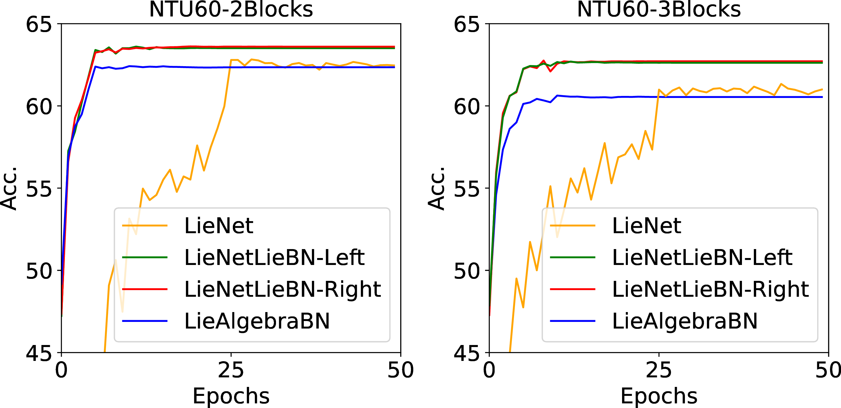
We compare LieAlgebraBN and LieBN under the LieNet backbone on the relatively large NTU60 dataset. Following the main paper, we adopt two-block and three-block architectures. We observe that LieAlgebraBN benefits from a decreasing learning rate upon convergence. Therefore, we apply the same learning rate schedule as in LieBN while keeping all other settings identical. 6 presents the testing accuracy curve, demonstrating that LieBN outperforms LieAlgebraBN under both architectures. This may be attributed to the fact that the Lie algebra, as a local tangent space approximation, distorts the intrinsic geometry of the Lie group, leading to suboptimal normalization.
15 Proofs↩︎
15.1 Proof of 1↩︎
Proof. Invariance: First, we note that all four Lie groups are commutative. Secondly, the construction of all four metrics is similar. It suffices to show the left-invariance of ECM.
We only need to show that \(L_{Q}: \mathcal{C}^{n}_{++} \to \mathcal{C}^{n}_{++}\) for any \(Q \in \mathcal{C}^{n}_{++}\) is a Riemannian isometry. \(L_{Q}\) can be rewritten as \[\begin{align} L_{Q} = \Theta^{-1} \circ \widetilde{L}_{\Theta(Q)} \circ \Theta, \end{align}\] where \(\widetilde{L}_{\Theta(Q)}\) is the left translation over \(\mathrm{LT}_1^{n}\), which is an isometry over \(\mathrm{LT}_1^{n}\). As \(\Theta^{-1}\), \(\widetilde{L}_{\Theta(Q)}\), and \(\Theta\) are all isometries, their composition is an isometry as well.
WFM: The WFM in the Euclidean space is reduced to arithmetic weighted average. By the isometry of \(f\), one can directly obtain the results. ◻
15.2 Proof of 2↩︎
Proof. Property [pro:mle95m]: The MLE of \(M\) is \[\begin{align} M_{\mathrm{MLE}} &= \operatorname{argmax}\log(K(v)) - \sum_{i=1}^N \frac{\operatorname{d}(P_i,M)^2}{2v^2}\\ &= \operatorname{argmin}\sum_{i=1}^N \operatorname{d}(P_i,M)^2. \end{align}\]
Property [pro:hom]: We denote \(Y=\operatorname{L}_B(X)\), and \(p_X\) and \(p_Y\) as the density of \(X\) and \(Y\), respectively. The density of \(Y\) is \[\begin{align} p_{Y}(Q) &\stackrel{(1)}{=}p_X(\operatorname{L}_{B^{-1}_{\odot}}(Q))\\ &= k(\sigma) \exp \left(-\frac{\operatorname{d}(\operatorname{L}_{B^{-1}_{\odot}}(Q), M)^2}{2 \sigma^2}\right)\\ &\stackrel{(2)}{=} k(\sigma) \exp \left(-\frac{\operatorname{d}(Q, \operatorname{L}_{B}(M))^2}{2 \sigma^2}\right). \end{align}\] The above comes from:
Thm. 7 in [58];
The isometry of the left translation.
◻
15.3 Proof of 3↩︎
Proof. The isometry of \(\operatorname{L}_B\) can directly obtain the homogeneity of the sample mean. Now let us focus on ?? . We have the following: \[\begin{align} \sum\nolimits_{i=1}^N w_i \operatorname{d}^2(\phi_{s}(P_i), E) &= \sum\nolimits_{i=1}^N w_i \|s\operatorname{Log}_E P_i\|_E\\ &= s^2\sum\nolimits_{i=1}^N w_i \|\operatorname{Log}_E P_i\|^2_E\\ &= s^2\sum\nolimits_{i=1}^N w_i \operatorname{d}^2(P_i, E), \end{align}\] where \(\| \cdot \|_{E}\) is the norm on \(T_E\mathcal{M}\). ◻
15.4 Proof of 6↩︎
Proof. As the right-invariant metric shares similar the left-invariant one, this proof follows the similar logic in the above two proofs.
Gaussian homogeneity: We denote \(Y=\operatorname{R}_B(X)\), and \(p_X\) and \(p_Y\) as the density of \(X\) and \(Y\), respectively. The density of \(Y\) is \[\begin{align} p_{Y}(Q) &\stackrel{(1)}{=}p_X(\operatorname{R}_{B^{-1}_{\odot}}(Q))\\ &= k(\sigma) \exp \left(-\frac{\operatorname{d}(\operatorname{R}_{B^{-1}_{\odot}}(Q), M)^2}{2 \sigma^2}\right)\\ &\stackrel{(2)}{=} k(\sigma) \exp \left(-\frac{\operatorname{d}(Q, \operatorname{R}_{B}(M))^2}{2 \sigma^2}\right). \end{align}\] The above comes from:
Thm. 13 in [58];
The isometry of the right translation.
Sample mean homogeneity: This is a direct corollary of the isometry of right translation. ◻
15.5 Proof of 7↩︎
Proof. As \(\mathbb{R}^{n}\) is an abelian group and the Euclidean inner product is bi-invariant, we focus on left-translation in the following. The core of this proof lies in the fact that on \(\mathbb{R}^{n}\), (1) the Fréchet mean and variance are reduced to the familiar Euclidean statistics. (2) the calculation of the running mean becomes the weighted arithmetic mean. (3) 10 11 12 become 4 ; We prove these three points one by one.
As stated by Luo et al [35], from the view of the product manifold, the element-wise Fréchet mean and variance on \(\mathbb{R}^{n}\) are equivalent to the vector-valued Euclidean variance and mean.
Besides, by similar proof as Luo et al [35], the weighted Fréchet mean on \(\mathbb{R}^{n}\) is simplified as the weighted arithmetic average. Therefore, on \(\mathbb{R}^{n}\), the calculation of running statistics in our 3 becomes the familiar moving average.
Thirdly, on \(\mathbb{R}^{n}\), we know that \(\operatorname{L}_x(y)=x+y\), \(\operatorname{Exp}_x v=x+v\), \(\operatorname{Log}_x y=y-x\), and the neutral element is \(0\). Since statistics, as well as the Euclidean BN, are calculated element-wisely, we can safely consider a single element, i.e.\(\mathbb{R}^{n}=\mathbb{R}\). For a batch of activations \(\{x_{i \ldots N} \in \mathbb{R}\}\), where the batch mean and batch variance are denoted as \(\mu_b\) and \(v^2_b\), then 10 11 12 are rewrote as: \[L_{\beta}\left( \operatorname{Exp}_0 \left[\frac{\gamma}{\sqrt{v^2_{b}+\epsilon}}\operatorname{Log}_0(\operatorname{L}_{-\mu_b}(x_i)) \right]\right) = \gamma \frac{x_i-\mu_{b}}{\sqrt{v^2_{b}+\epsilon}} + \beta.\] The above equation is the exact core computation of the standard Euclidean BN. ◻
15.6 Proof of 8↩︎
Proof. We first prove the case of \((\theta,\alpha,\beta)\text{-LEM}\), and then proceed to the case of \(\theta\text{-LCM}\).
\((\theta,\alpha,\beta)\text{-LEM}\): For clarity, we denote the metric tensor of \((\theta,\alpha,\beta)\text{-LEM}\) as \[g^{(\theta,\alpha,\beta)\text{-LE}}= \frac{1}{\theta^2}\operatorname{P}_\theta^*g^{(\alpha,\beta)\text{-LE}},\] where \(g^{(\alpha,\beta)\text{-LE}}\) is the metric tensor of \((\alpha,\beta)\text{-LEM}\). Let \(P \in \mathcal{S}^{n}_{++}\) and \(V,W \in T_P\mathcal{S}^{n}_{++}\), then we have \[\begin{align} g^{(\theta,\alpha,\beta)\text{-LE}}_P(V,W) &= \frac{1}{\theta^2} g^{(\alpha,\beta)\text{-LE}}_{\operatorname{P}_{\theta}(P)} \left(\operatorname{P}_{\theta*,P}(V),\operatorname{P}_{\theta*,P}(W) \right)\\ &= \frac{1}{\theta^2} \langle \left( \operatorname{log}\circ \operatorname{P}_{\theta} \right)_{*,P} (V), \left( \operatorname{log}\circ \operatorname{P}_{\theta} \right)_{*,P} (W) \rangle^{(\alpha,\beta)}\\ &= \langle \operatorname{log}_{*,P} (V), \operatorname{log}_{*,P} (W) \rangle^{(\alpha,\beta)}\\ &= g^{(\alpha,\beta)\text{-LE}}_P(V,W). \end{align}\]
\(\theta\text{-LCM}\): Let us first review a well-known fact of deformed metrics [90]. Let \(\tilde{g}=\frac{1}{\theta^2}\operatorname{P}_{\theta}^*g\) be the power-deformed metric on SPD Then when \(\theta\) tends to 0, for all \(P \in \mathcal{S}^{n}_{++}\) and all \(V \in T_P\mathcal{S}^{n}_{++}\), we have \[\label{eq:deformed95g95lim} \tilde{g}_P(V,V) \to g_{I}(\log_{*,P}(V),\log_{*,P}(V)).\tag{33}\]
By 33 , we can readily obtain the results. ◻
15.7 Proof of 9↩︎
Proof. \((\alpha,\beta)\text{-AIM}\) is left-invariant [3]. As the pullback of \((\alpha,\beta)\text{-AIM}\), \((\theta,\alpha,\beta)\text{-AIM}\) is left-invariant as well. Besides, Chen et al [69] shows that LCM is the pullback metric from the Euclidean space of \(\mathrm{LT}^{n}\). Therefore, \(\theta\)-LCM is bi-invariant. ◻
15.8 Proof of 10↩︎
Proof. In the following, we denote the \(\operatorname{d}^{\mathrm{L}}\), \(\operatorname{Log}^{\mathrm{L}}\), \(\operatorname{Exp}^{\mathrm{L}}\) as the Riemannian operators under the left-invariant metric, i.e.AIM. Note that the Cholesky decomposition pulls back the group operation of matrix product from the Cholesky manifold \(\mathrm{LT}_{++}^{n}\) [3]. For simplicity, we abbreviate \(\odot^{\mathrm{AI}}\) as \(\odot\).
Let us first review the differential map of Cholesky decomposition and its inverse [37]. Following the notations in this theorem and further denote \(X \in T_L\mathrm{LT}_{++}^{n}\), we have the following \[\begin{align} \tag{34} \operatorname{Chol}_{*,P} (V) &= L\left(L^{-1} V L^{-\top}\right)_{\frac{1}{2}},\\ \tag{35} (\operatorname{Chol}^{-1})_{*,L} (X) &= L X^{\top}+X L^{\top}. \end{align}\] Specifically, for the differential map at \(I\), we have \[\begin{align} \tag{36} \operatorname{Chol}_{*,I} (V) &= \left( V \right) _{\frac{1}{2}}, \forall V \in T_I\mathcal{S}^{n}_{++}.\\ \tag{37} (\operatorname{Chol}^{-1})_{*,I} (X) &= \left(X \right)_{\mathrm{Sym}}, \forall X \in T_I\mathrm{LT}_{++}^{n}. \end{align}\] Denoting \(\widetilde{\operatorname{L}}\) and \(\widetilde{\operatorname{R}}\) as the group translation on the Cholesky manifold \(\mathrm{LT}_{++}^{n}\), we have the following w.r.t. the differential maps of left and right translation: \[\begin{align} \notag \left(\operatorname{L}_{P,* {P}^{-1}_{\odot}} \right)^{-1} & \stackrel{(1)}{=} \left( \left( \operatorname{Chol}^{-1} \right)_{*, I} \widetilde{\operatorname{L}}_{L *, L^{-1}} \circ \operatorname{Chol}_{*, {P}^{-1}_{\odot}} \right)^{-1}\\ \tag{38} & = \left( \operatorname{Chol}_{*, {P}^{-1}_{\odot}} \right)^{-1} \left( \widetilde{\operatorname{L}}_{L *, L^{-1}} \right)^{-1} \circ \operatorname{Chol}_{*, I},\\ \tag{39} \operatorname{R}_{{P}^{-1}_{\odot} *,P} & \stackrel{(2)}{=} \left(\operatorname{Chol}^{-1}\right)_{*, I} \circ \widetilde{\operatorname{R}}_{L^{-1} *, L} \circ \operatorname{Chol}_{*, P}. \end{align}\] The above derivation comes from the following:
\(\operatorname{L}_P = \operatorname{Chol}^{-1} \circ \widetilde{\operatorname{L}}_L \circ \operatorname{Chol}\);
\(\operatorname{R}_{{P}^{-1}_{\odot}} = \operatorname{Chol}^{-1} \circ \widetilde{\operatorname{R}}_{L^{-1}} \circ \operatorname{Chol}\).
Riemannian metric: For the differential of right translation, we have the following \[\label{eq:diff95rtrans95spd} \begin{align} \operatorname{R}_{{P}^{-1}_{\odot} *,P} (V) & = \left(\operatorname{Chol}^{-1}\right)_{*, I} \circ \widetilde{\operatorname{R}}_{L^{-1} *, L} \circ \operatorname{Chol}_{*, P} (V) \\ & = \left( L(L^{-1} V L^{-\top})_{\frac{1}{2}} L^{-1} \right)_{\mathrm{Sym}}. \\ \end{align}\tag{40}\] By 40 , one can obtain the expression for the Riemannian metric tensor.
Riemannian geodesic and exponential map: According to [91], we have the following for the operators between left- and right-invariant metrics: \[\begin{align} \tag{41} \operatorname{Exp}_{P} (V) &= \left\{ \operatorname{Exp}^{\mathrm{L}}_ {P^{-1}_{\odot}} \left( -\left(\operatorname{L}_{P,*P^{-1}_{\odot}} \right)^{-1} \circ \operatorname{R}_{P^{-1}_{\odot}*,P} (V) \right) \right\}^{-1}_{\odot},\\ \tag{42} \operatorname{d}(P,Q) &= \operatorname{d}^{\mathrm{L}} \left( {P}^{-1}_{\odot}, {Q}^{-1}_{\odot}\right). \end{align}\] Putting the AIM-based geodesic distance into the RHS of 42 , one can obtain the geodesic distance under CRIM.
Now, we simplify 41 . Putting 38 39 into 41 , we have the following: \[\label{eq:exp95crim95derivation} \begin{align} \operatorname{Exp}_{P}(V) & = \left\{ \operatorname{Exp}^{\mathrm{L}}_{{P}^{-1}_{\odot}} \left(- \left( \operatorname{Chol}_{*, {P}^{-1}_{\odot}} \right)^{-1} \circ \left( \widetilde{\operatorname{L}}_{L *, L^{-1}} \right)^{-1} \circ \widetilde{\operatorname{R}}_{L^{-1} *, L} \circ \operatorname{Chol}_{*, P} (V) \right) \right\}_{\odot} ^{-1} \\ & = \left\{ \operatorname{Exp}^{\mathrm{L}}_{{P}^{-1}_{\odot}} \left(- \left( \operatorname{Chol}_{*, {P}^{-1}_{\odot}} \right)^{-1} \left[ L^{-1} \operatorname{Chol}_{*, P} (V) L^{-1} \right] \right) \right\}_{\odot} ^{-1} \\ & \stackrel{(1)}{=} \left\{ \operatorname{Exp}^{\mathrm{L}}_{{P}^{-1}_{\odot}} \left(- \left( \operatorname{Chol}_{*, {P}^{-1}_{\odot}} \right)^{-1} \left[ \left(L^{-1} V L^{-\top}\right)_{\frac{1}{2}} L^{-1} \right] \right) \right\}_{\odot} ^{-1} \\ & \stackrel{(2)}{=} \left\{ \operatorname{Exp}^{\mathrm{L}}_{{P}^{-1}_{\odot}} \left(- \left( \left(L^{-1} V L^{-\top}\right)_{\frac{1}{2}} L^{-1} L^{-\top} \right)_{\mathrm{Sym}} \right) \right\}_{\odot} ^{-1}.\\ \end{align}\tag{43}\] The above comes from the following:
Riemannian logarithm: From the second equality in 43 , we have the following \[\label{eq:log95crim95derivation} \begin{align} \operatorname{Log}_P (Q) &= - \operatorname{Chol}_{*, P}^{-1} \left\{ L\operatorname{Chol}_{*, {P}^{-1}_{\odot}} \left(\operatorname{Log}^\mathrm{L}_{{P}^{-1}_{\odot}} \left({Q}^{-1}_{\odot} \right) \right) L \right\}\\ &\stackrel{(1)}{=} - \operatorname{Chol}_{*, P}^{-1} \left\{ \left(L \widetilde{V} L^\top \right)_{\frac{1}{2}} L \right\}\\ &= -\left(L L^{\top} \left( L \widetilde{V}L^{\top} \right)_{\frac{1}{2}}^{\top} \right)_{\mathrm{Sym}} \end{align}\tag{44}\] The above comes from the following:
- \(\operatorname{Chol}_{*,{P}^{-1}_{\odot}} (V) = L^{-1} \left(L V L^\top\right)_{\frac{1}{2}}, \forall V \in T_{{P}^{-1}_{\odot}}\mathcal{S}^{n}_{++}\).
◻
15.9 Proof of 1↩︎
Proof. Completeness: 14 indicates that \(\operatorname{Exp}_{I}\) is defined over the whole \(T _I \mathcal{S}^{n}_{++}\). Besides, the SPD manifold is connected [50]. By Cor. 6.20 in [43], CRIM is complete.
Geodesic: For simplicity, we abbreviated \(\odot^{\mathrm{AI}}\) as \(\odot\). The geodesic connecting \(P\) and \(Q\) can be obtained by the following: \[\begin{align} \gamma{(t; P,Q)} &= \operatorname{Exp}_{P} \left( t\operatorname{Log}_{P} (Q)\right)\\ &\stackrel{(1)}{=} \left\{ \operatorname{Exp}^{\mathrm{L}}_{{P}^{-1}_{\odot}} \left(- \left( \operatorname{Chol}_{*, {P}^{-1}_{\odot}} \right)^{-1} \left[ L^{-1} \operatorname{Chol}_{*, P} \left(t \operatorname{Log}_P (Q) \right) L^{-1} \right] \right) \right\}_{\odot} ^{-1} \\ &\stackrel{(2)}{=} \left\{ \operatorname{Exp}^{\mathrm{L}}_{{P}^{-1}_{\odot}} \left( t\operatorname{Log}^\mathrm{L}_{{P}^{-1}_{\odot}} \left({Q}^{-1}_{\odot} \right) \right) \right\}_{\odot} ^{-1} \\ &= \left\{ \gamma^{\mathrm{AI}}(t; \widetilde{P},\widetilde{Q}) \right\}_{\odot} ^{-1}. \\ \end{align}\] The above comes from the following:
◻
15.10 Proof of 12↩︎
Proof. With out loss of generality, we focus on the case of the left-invariant metric. The results of the right-invariant metric can be proven similarly.
We denote 10 11 12 on \(\mathcal{M}_i, i=1,2\) as the mapping \(\xi^i(\cdot | M,v^2,B,s)\). Let \(\mathcal{B}=\{P_{1 \ldots N}\}\) and \(f(\mathcal{B})=\{f(P_{1 \ldots N})\}\).
The core of this proof lies in three points:
The Fréchet mean and variance of \(\mathcal{B}\) in \(\mathcal{M}_1\) correspond to the counterparts of \(f(\mathcal{B})\) in \(\mathcal{M}_2\).
\(\xi^1(P_i|M,v^2,B,s)\) in \(\mathcal{M}_1\) is equal to \(f^{-1} (\xi^2(f(P_i)|f(M),v^2,f(B),s))\).
The updates of running statistics in \(\mathcal{M}_1\) correspond to the counterparts in \(\mathcal{M}_2\).
We denote \(M\) as the Fréchet mean of \(\mathcal{B}\), and \(v^2\) as the Fréchet variance of \(\mathcal{B}\). Then, by the isometry of \(f\), the Fréchet mean and variance of \(f(\mathcal{B})\) are \(f(M)\) and \(v^2\), respectively.
On \(\mathcal{M}_i, i=1,2\), we denote \(\operatorname{L}^i, \odot^i, \operatorname{Exp}^i,\operatorname{Log}^i\) as the Lie group and Riemannian operators, \(E^i\) as the neutral element, and 11 as \(\phi^i_s(\cdot)\). With the isometry and Lie group isomorphism of \(f\), we have the following equations: \[\begin{align} L^1_{M^{-1}_{\odot^1}} &=f^{-1} \circ \operatorname{L}^2_{f(M)^{-1}_{\odot^2}} \circ f,\\ \notag \phi^1_{s} &=\operatorname{Exp}^1_{E^1}\left[ s \operatorname{Log}^1_{E^1}(\cdot) \right]\\ \notag &= f^{-1} \left( \operatorname{Exp}^{1}_{E^2}\left[ s \operatorname{Log}^2_{E^2}(f(\cdot))\right]\right)\\ &= f^{-1} \circ \phi^2_s \circ f,\\ L^1_{B} &=f^{-1} \circ \operatorname{L}^2_{f(B)} \circ f. \end{align}\] Then we have \[\label{eq:core95ops95pm} \xi^1(P_i|M,v^2,B,s)=f^{-1}(\xi^2(f(P_i)|f(M),v^2,f(B),s))\tag{45}\]
Lastly, we show the correspondence between running statistics. Since the Fréchet variance is the same for both \(\mathcal{B}\) and \(f(\mathcal{B})\), we focus on the running mean. Let \(M_r\) and \(f(M_r)\) denote the initial values of the running means in \(\mathcal{M}_1\) and \(\mathcal{M}_2\) respectively, and \(\operatorname{WFM}^i\) represent the weighted Fréchet mean in \(\mathcal{M}_i\). Then the updated running mean in \(\mathcal{M}_1\) is \[\operatorname{WFM}^1(\{1-\gamma,\gamma\},\{M_r,M\})= f^{-1}(\operatorname{WFM}^2(\{1-\gamma,\gamma\},\{f(M_r),f(M)\}))\] we can further simply the above equation as \[\label{eq:wfm95pm} \operatorname{WFM}^1 = f^{-1} \circ \operatorname{WFM}^2 \circ f\tag{46}\]
Denoting \(\operatorname{LieBN}^i\) as the LieBN algorithm on \(\mathcal{M}_i\), 45 and 46 imply that: \[\operatorname{LieBN}^1(P_i|B,s,\epsilon,\gamma)=f^{-1} \left[\operatorname{LieBN}^2(f(P_i)|f(B),s,\epsilon,\gamma) \right].\] ◻
References↩︎
Although some metrics are bi-invariant, the associated group structures are commutative [36], [37]. Therefore, their bi-invariance is reduced to left-invariance.↩︎
Although not discussed in [32], 5 6 as congruent actions can transfer the batch mean into desirable one under AIM.↩︎
The neutral element \(E\) is not necessarily the identity matrix.↩︎
Each block consists of a RotMap layer followed by a RotPooling layer. For more details, please refer to [10].↩︎
This should be more precisely understood as the determinant of the matrix representation of \(L_{P*, E}\) under a local coordinate↩︎
https://github.com/rkobler/TSMNet↩︎
https://proceedings.neurips.cc/paper_files/paper/2019/file/6e69ebbfad976d4637bb4b39de261bf7-Supplemental.zip↩︎