Sticky Routing: Training MoE Models for Memory-Efficient Inference
June 12, 2026
Abstract
Mixture-of-Experts (MoE) models activate only a sparse subset of experts per token, yet consecutive tokens frequently activate different experts—causing constant weight swapping between slow storage and fast memory on edge devices. Existing remedies are either system-level (caching heuristics) or post-hoc (router fine-tuning), leaving the root cause unchanged during pretraining. We propose StickyMoE, a differentiable routing consistency loss that penalises abrupt expert switches between adjacent tokens, encouraging the router to maintain the same expert assignment across semantically coherent spans. StickyMoE requires no architectural changes, adds a single hyperparameter \(\lambda\), and unlike post-hoc methods, allows expert representations and routing decisions to co-adapt from the first training step. Experiments on small and medium MoE language models show that StickyMoE reduces the expert switch rate by up to 59% while simultaneously improving perplexity on the medium model, and reduces cache misses by up to \(\mathbf{3.92\times}\), Pareto-dominating post-hoc fine-tuning on the quality–locality frontier. Routing temporal locality is most efficiently instilled at training time. Code is available at: https://github.com/alikayyam/sticky_moe.git.
1 Introduction↩︎
The Mixture-of-Experts (MoE) architecture has emerged as one of the most practically important techniques for scaling large language models (LLMs) without a proportional increase in per-token computation [1]–[3]. By replacing dense feed-forward network (FFN) sublayers with a collection of \(N\) expert FFNs and a learned sparse router, MoE models can possess billions of parameters while activating only a small subset—typically 1 or 2 experts out of 8–128—for each input token. This property makes MoE architectures theoretically attractive for edge deployment: if only 2 of 64 experts need to be resident in fast memory at any moment, the effective working-set size is a small fraction of the total parameter count.
1.0.0.1 The expert-swapping problem.
In practice, this promise is undermined by the temporal inconsistency of standard MoE routers. Because the router makes an independent routing decision for every token based solely on that token’s hidden representation, consecutive tokens in a sequence routinely activate entirely different experts [4]. On a system with limited GPU VRAM or on-device SRAM, each such switch requires evicting the currently cached expert weights and loading new ones from CPU RAM or flash storage. PCIe and NVMe bandwidth is one to two orders of magnitude lower than GPU memory bandwidth; a single expert weight transfer can therefore dominate the latency of the forward pass itself [5], [6]. The result is that MoE models, despite their theoretical sparsity advantage, can be slower than comparably-sized dense models on memory-constrained hardware.
1.0.0.2 Why existing solutions are insufficient.
Prior work addresses this problem from two directions. System-level approaches maintain an expert cache in fast memory and use eviction policies (LRU, LFU) or learned prefetchers to reduce cache miss rates [5], [7], [8]. While practically useful, these methods are fundamentally reactive: they try to exploit whatever locality the model’s router happens to produce, but cannot improve routers that are intrinsically inconsistent. Post-hoc approaches fine-tune only the router of an already-trained model to increase expert reuse [9], which is more targeted but still treats the symptom rather than the cause: the expert representations have already been shaped by a training regime that never incentivised locality, and a brief fine-tuning pass can only partially re-align the routing surface. A third line of work, most closely represented by Oracle-MoE [4], redesigns the routing architecture so that the router operates in an attention-derived “oracle space” that is inherently more semantically stable across tokens. Oracle-MoE trains from scratch, which is a step in the right direction, but the locality property is structural—embedded in the choice of routing input—rather than explicitly optimised. We propose a different approach: StickyMoE, which instils routing locality directly as a training objective, requiring no architectural changes and no post-hoc correction.
1.0.0.3 Our proposal.
We argue that the cleanest and most general solution is to treat routing temporal locality as an explicit training objective. Specifically, we introduce a routing consistency loss — a differentiable \(\ell_2\) penalty on consecutive gate distributions — to directly optimise for temporal locality in MoE routing: \[\mathcal{L}_{\text{cons}} \;=\; \frac{1}{T-1}\sum_{t=2}^{T} \bigl\| \mathbf{g}_{t} - \mathbf{g}_{t-1} \bigr\|_2^2, \label{eq:cons95loss95intro}\tag{1}\] where \(\mathbf{g}_t \in \mathbb{R}^N\) is the softmax gate probability vector produced by the router for token \(t\) and \(T\) is the sequence length. The total training loss is \[\mathcal{L}= \mathcal{L}_{\text{CE}} + \lambda\,\mathcal{L}_{\text{cons}} + \mu\,\mathcal{L}_{\text{bal}}, \label{eq:total95loss95intro}\tag{2}\] where \(\mathcal{L}_{\text{CE}}\) is the standard cross-entropy language modelling loss, \(\mathcal{L}_{\text{bal}}\) is the load-balancing auxiliary loss from [2], and \(\lambda, \mu \geq 0\) are scalar hyperparameters. This formulation:
requires no architectural modification—it applies to any standard top-\(k\) MoE without changing the router structure;
is differentiable everywhere and adds negligible computational overhead;
is architecture-agnostic, attaching equally to small experimental models and large-scale MoEs;
co-trains with the language modelling objective, so that expert representations and routing decisions co-evolve toward local consistency from the very first update.
1.0.0.4 Contributions.
We make the following specific contributions:
We propose the routing consistency loss, a simple differentiable training objective that directly penalises expert switching between adjacent tokens, requiring no architectural changes and adding a single hyperparameter \(\lambda\) (4).
We show empirically that \(\mathcal{L}_{\text{cons}}\) and \(\mathcal{L}_{\text{bal}}\) are complementary: expert utilisation entropy remains above \(1.92\) bits out of \(\log_2 4 = 2.0\) bits across all settings, confirming that the consistency loss does not induce expert collapse (5).
We propose a soft-hard variant that addresses long-range routing drift by combining the per-step soft penalty with a segment-level anchor constraint, achieving stronger locality guarantees without additional quality cost (4).
We present controlled experiments on small and medium MoE language models trained on WikiText-2, comparing against a vanilla MoE baseline, a Hard-Window ablation, a simulated ReMoE post-hoc baseline, and a simplified Oracle-MoE reimplementation, measuring perplexity, switch rate, cache hit rate, and utilisation entropy (5).
1.0.0.5 Paper organisation.
2 reviews MoE architectures and the expert-swapping bottleneck. 3 surveys related work and positions StickyMoE precisely. 4 presents the method in full detail. 5 describes the experimental setup and presents results. 6 discusses findings, limitations, and broader implications. 7 concludes and outlines future directions.
2 Background↩︎
2.1 Mixture-of-Experts Language Models↩︎
A standard MoE transformer replaces each FFN sublayer with a collection of \(N\) expert networks \(\{\mathcal{E}_i\}_{i=1}^{N}\) and a router \(\mathcal{R}\). Given the hidden representation \(\mathbf{h}_t \in \mathbb{R}^d\) of token \(t\), the router computes gate logits \(\boldsymbol{\ell}_t = \mathbf{W}_r \mathbf{h}_t \in \mathbb{R}^N\) and selects the top-\(k\) experts by probability: \[\begin{align} \mathbf{g}_t &= \mathrm{softmax}(\boldsymbol{\ell}_t), \tag{3} \\ \mathcal{S}_t &= \mathrm{top}\text{-}k(\mathbf{g}_t), \tag{4} \\ \mathbf{y}_t &= \sum_{i \in \mathcal{S}_t} g_{t,i}\, \mathcal{E}_i(\mathbf{h}_t). \tag{5} \end{align}\] The router weight matrix \(\mathbf{W}_r \in \mathbb{R}^{N \times d}\) is the only additional parameter relative to a dense FFN layer. The expert networks \(\mathcal{E}_i\) are typically two-layer FFNs with the same structure as the dense FFN they replace.
2.2 Load-Balancing Auxiliary Loss↩︎
Without explicit regularisation, MoE routers tend to collapse: a small subset of experts receives disproportionately many tokens, while the remainder are rarely activated and fail to develop useful representations [2]. To prevent this, we include the standard load-balancing auxiliary loss: \[\mathcal{L}_{\text{bal}} = N \sum_{i=1}^{N} f_i \cdot p_i, \label{eq:bal95loss}\tag{6}\] where the sum is over all \(N\) experts, \(f_i\) is the fraction of top-\(k\) assignments to expert \(i\) (counting all \(k\) slots), and \(p_i = \frac{1}{T}\sum_{t=1}^{T} g_{t,i}\) is the mean gate probability assigned to expert \(i\), both computed over the current batch. The product \(f_i \cdot p_i\) is minimised when routing is uniform across experts; scaling by \(N\) ensures the loss magnitude is independent of the number of experts.
2.3 Expert Swapping on Memory-Constrained Hardware↩︎
Let \(M_{\text{fast}}\) denote the fast-memory capacity (VRAM or on-device SRAM) and \(w_e\) the size of a single expert’s weight tensor. A device can hold at most \(\lfloor M_{\text{fast}} / w_e \rfloor\) expert weight matrices simultaneously alongside the attention and embedding parameters. When the router at decoding step \(t\) selects an expert not currently in fast memory, the system must evict a cached expert and load the new one from slow memory—a cache miss. The per-step latency is: \[\tau_t = \tau_{\text{compute}} + \mathbb{1}[\text{miss}_t]\cdot\tau_{\text{load}},\] where \(\tau_{\text{load}} \gg \tau_{\text{compute}}\) on bandwidth-limited devices. The expected fraction of steps that incur a cache miss is determined by the expert switch rate: \[\text{SR} = \frac{1}{T-1}\sum_{t=2}^{T} \mathbb{1}[\mathcal{S}_t \neq \mathcal{S}_{t-1}]. \label{eq:switch95rate}\tag{7}\] This single-sequence definition illustrates the concept; the full empirical estimator averaging over layers is defined formally in 5. Reducing SR is therefore directly equivalent to reducing expected inference latency under memory constraints.
3 Related Work↩︎
3.1 System-Level Expert Offloading↩︎
A large body of work treats expert weights as a two-level memory hierarchy and focuses on minimising the latency cost of loading experts from slow to fast memory at inference time. MoE-Infinity [5] introduces a sparsity-aware expert cache on personal machines, keeping attention weights in GPU memory and streaming expert weights from host RAM. Fiddler [7] uses the CPU itself for expert computation to avoid PCIe transfers. DuoServe [8] separately optimises prefill and decode phases using a learned prediction model for expert activation paths. EdgeMoE [6] proposes importance-driven expert scheduling specifically for edge settings. A related thread in the literature studies locality in deployed models: [10] conduct an empirical study showing that local routing consistency varies dramatically across model families, and that some models are fundamentally ill-suited to offloading-based deployment.
All of the above methods are inference-time interventions. They exploit whatever locality the trained model’s router provides but cannot alter the router’s inductive bias. StickyMoE is orthogonal and complementary: it can be used in conjunction with any of these systems, supplying a router that already tends toward consistency.
3.2 Post-Hoc Router Adaptation↩︎
ReMoE [9] is the most directly related post-hoc method. It fine-tunes only the router parameters of a pretrained MoE checkpoint to increase short-horizon expert reuse, using a combination of the language modelling loss and a locality-aware regulariser on the gate distribution. ReMoE reports meaningful reductions in cache miss rate and throughput improvements in vLLM-based serving. Its key advantage is practicality: it can be applied to any pretrained model without retraining from scratch. Its key limitation is that the expert representations themselves are fixed—shaped by a training process that never incentivised locality—so the router is being asked to change its decisions in a representation space that was not designed with locality in mind. StickyMoE avoids this mismatch by instilling the locality bias from the first training step, allowing the expert representations and routing decisions to co-adapt. In our controlled experiments, we were unable to reproduce meaningful SR reductions from post-hoc router fine-tuning; we attribute this to the representation mismatch discussed in 6.
3.3 Training-Time Architectural Redesign↩︎
Oracle-MoE [4] is the closest prior work to ours in motivation and in training regime. It identifies the same root cause—temporal routing inconsistency—and proposes a structural solution: routing tokens not in the standard hidden-state space but in an “oracle space” derived from attention scores, which is empirically more semantically stable across consecutive tokens. Oracle-MoE is trained from scratch and achieves state-of-the-art inference speed on edge devices without sacrificing task performance. However, it requires a non-trivial architectural modification (replacing the router input with attention-derived features), making it harder to apply to existing architectures and training pipelines. StickyMoE achieves comparable locality through a lightweight auxiliary loss that requires no architectural change, making it more accessible and easier to combine with other MoE innovations.
3.4 Routing Regularisation in MoE↩︎
The Switch Transformer [2] and ST-MoE [11] introduce load-balancing losses to prevent expert collapse. Expert Choice routing [12] inverts the routing direction to guarantee balanced utilisation. These works regularise the spatial distribution of routing decisions across tokens in a batch, but do not address the temporal coherence of routing across adjacent tokens in a sequence. Our consistency loss is orthogonal to and composable with all of these.
3.5 Temporal Coherence in Related Architectures↩︎
Mixture of Depths [13] routes tokens to skip layers entirely, creating a different form of computation-aware sparse routing. Pre-gated MoE [14] predicts which experts will be needed before the full computation, enabling prefetch to hide loading latency. Neither method explicitly trains for inter-token routing consistency, but both share the broader goal of reducing unnecessary computation or memory movement. In the time-series domain, [15] assigns experts to predetermined temporal segments based on known signal physics—a hard form of the stickiness we achieve through soft regularisation.
3.6 Summary of Differences↩︎
1 provides a structured comparison of StickyMoE with the most relevant prior works along the dimensions most pertinent to edge deployment.
5pt
4 Method↩︎
4.1 Routing Consistency Loss↩︎
Let \(L\) denote the number of MoE layers in the model. For layer \(\ell\) and a sequence of \(T\) tokens, let \(\mathbf{g}_t^{(\ell)} \in \mathbb{R}^N\) be the softmax gate probability vector produced by the router of layer \(\ell\) for token \(t\). We define the per-layer consistency loss as: \[\mathcal{L}_{\text{cons}}^{(\ell)} \;=\; \frac{1}{T-1}\sum_{t=2}^{T} \bigl\| \mathbf{g}_t^{(\ell)} - \mathbf{g}_{t-1}^{(\ell)} \bigr\|_2^2. \label{eq:cons95loss}\tag{8}\] The full consistency loss aggregates over all MoE layers: \[\mathcal{L}_{\text{cons}} \;=\; \frac{1}{L}\sum_{\ell=1}^{L} \mathcal{L}_{\text{cons}}^{(\ell)}. \label{eq:cons95loss95full}\tag{9}\]
4.1.0.1 Interpretation.
The \(\ell_2\) distance between consecutive gate distributions \(\mathbf{g}_t\) and \(\mathbf{g}_{t-1}\) is zero if and only if the router assigns identical probability mass to all experts for both tokens. Minimising \(\mathcal{L}_{\text{cons}}\) therefore directly penalises abrupt changes in the routing distribution. Because \(\mathbf{g}_t\) is a probability simplex vector, the maximum possible value of \(\|\mathbf{g}_t - \mathbf{g}_{t-1}\|_2^2\) is \(2\) (when one token is routed entirely to expert \(i\) and the next entirely to expert \(j \neq i\)). The loss thus has a natural \([0, 2]\) range, making \(\lambda\) interpretable across different model sizes and expert counts.
4.1.0.2 Gradient flow.
The gate probabilities \(\mathbf{g}_t = \mathrm{softmax}(\mathbf{W}_r \mathbf{h}_t)\) are differentiable in both \(\mathbf{W}_r\) (the router weight) and \(\mathbf{h}_t\) (the input hidden state). Minimising \(\mathcal{L}_{\text{cons}}\) therefore:
directly updates \(\mathbf{W}_r\) to produce more similar gate distributions for semantically adjacent tokens, and
backpropagates through \(\mathbf{h}_t\) into the preceding attention and embedding layers, encouraging the model to produce hidden representations whose local geometry is better aligned with the router’s decision boundaries.
This second effect is the key advantage over post-hoc router fine-tuning: StickyMoE trains the representation as well as the routing function to be locally consistent.
4.2 Total Training Objective↩︎
The full training loss is: \[\mathcal{L}\;=\; \mathcal{L}_{\text{CE}} + \lambda\,\mathcal{L}_{\text{cons}} + \mu\,\mathcal{L}_{\text{bal}}, \label{eq:total95loss}\tag{10}\] where \(\mathcal{L}_{\text{CE}}\) is the standard next-token cross-entropy loss, \(\mathcal{L}_{\text{bal}}\) is the load-balancing loss from 6 , and \(\lambda, \mu \geq 0\) are hyperparameters. We recommend \(\mu = 0.01\) following [2] and treat \(\lambda\) as the primary experimental variable.
4.3 Interaction with Load Balancing↩︎
A natural concern is whether \(\mathcal{L}_{\text{cons}}\) and \(\mathcal{L}_{\text{bal}}\) conflict: a trivial minimiser of \(\mathcal{L}_{\text{cons}}\) is to route all tokens to the same expert, which would eliminate switching but collapse expert diversity. In practice, \(\mathcal{L}_{\text{bal}}\) effectively prevents this. For all \(\lambda \leq 0.5\) explored in our experiments, utilisation entropy remains above \(1.92\) bits out of a maximum of \(\log_2 4 = 2.0\) bits, confirming that expert usage stays near-uniform throughout training (see 6 7). The two objectives are therefore complementary in the regime we consider: \(\mathcal{L}_{\text{cons}}\) shapes when experts are used across the sequence, while \(\mathcal{L}_{\text{bal}}\) ensures which experts are used remains balanced.
4.4 Soft-Hard Variant↩︎
The soft consistency loss enforces a chain constraint: each token is penalised for differing from its immediate predecessor. While effective at suppressing abrupt local switches, this formulation is vulnerable to gradual drift — the router may take small steps at each transition yet migrate far from its starting expert over a long span, incurring cache misses that the per-step penalty never directly penalises.
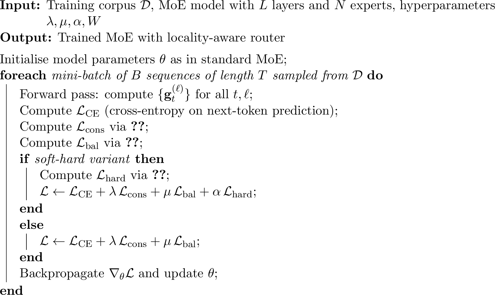
To address this, we introduce a complementary anchor constraint, inspired by commitment losses in discrete representation learning [16]. The sequence is partitioned into non-overlapping windows of \(W\) tokens. The first token of each window routes freely; its gate distribution \(\mathbf{g}_{s(t)}^{(\ell)}\) then becomes a fixed anchor for the remainder of the window. Every subsequent token is penalised for deviating from this anchor, with the penalty weight increasing linearly with distance from the window start: \[\begin{align} \mathcal{L}_{\text{hard}}^{(t,\ell)} &\;=\; \frac{t - s(t)}{W} \cdot \bigl\| \mathbf{g}_t^{(\ell)} - \mathbf{g}_{s(t)}^{(\ell)} \bigr\|_2^2, \\[4pt] \mathcal{L}_{\text{hard}} &\;=\; \frac{1}{LT} \sum_{\ell=1}^{L} \sum_{t=1}^{T} \mathcal{L}_{\text{hard}}^{(t,\ell)}, \end{align} \label{eq:hard95loss}\tag{11}\] where \(s(t) = W \lfloor t/W \rfloor\) is the start of the window containing token \(t\). Anchor tokens (where \(t = s(t)\)) contribute zero through the \(\frac{t - s(t)}{W}\) factor and require no special treatment. The sum over layers mirrors the aggregation in \(\mathcal{L}_{\text{cons}}\) (9 ), ensuring the hard loss operates uniformly across all MoE layers. The linear ramp is a deliberate design choice: early in the window the correct expert for the segment is uncertain, so flexibility is preserved; by the window’s end the router should be fully committed. At window boundaries the anchor resets and the router is free to reassign without penalty.
The soft and hard losses are geometrically complementary. The soft loss controls the step size of routing changes — each transition is small. The hard loss controls the radius of routing changes — every token stays close to the window anchor. A small-step path can still drift far from its origin; a radius constraint alone does not prevent jagged local switching within the window. Together they enforce both fine-grained smoothness and coarse-grained commitment, which is precisely what a memory-constrained cache requires: not just that adjacent tokens agree, but that an entire span can be served by the same resident expert.
The total training loss for the soft-hard variant is: \[\mathcal{L}\;=\; \mathcal{L}_{\text{CE}} + \lambda\,\mathcal{L}_{\text{cons}} + \mu\,\mathcal{L}_{\text{bal}} + \alpha\,\mathcal{L}_{\text{hard}}, \label{eq:total95loss95softhard}\tag{12}\] where \(\lambda\), \(\mu\), and \(\alpha\) are scalar hyperparameters controlling the relative weight of the consistency, load-balancing, and anchor terms respectively. Setting \(\alpha = 0\) recovers the soft-only objective in 10 .
4.5 Algorithm↩︎
Algorithm 1 summarizes the StickyMoE training procedure.
5 Experiments↩︎
5.1 Dataset↩︎
All experiments use the WikiText-2 raw character dataset [17] (wikitext-2-raw-v1), a standard language modelling
benchmark derived from verified Good and Featured Wikipedia articles. We use the raw (un-tokenised) variant to avoid pre-processing artefacts. Text is tokenised with the GPT-2 byte-pair encoding (BPE) vocabulary [18] using the GPT2Tokenizer from the HuggingFace Transformers library [19], yielding a vocabulary of \(|\mathcal{V}| = 50{,}257\) tokens. Each split is tokenised as a single flat sequence; document boundaries are not marked with
special tokens.
| Split | Documents | Tokens |
|---|---|---|
| Train | 36,718 | 2,347,038 |
| Validation | 3,760 | 242,643 |
| Test | 4,358 | 273,768 |
5.1.0.1 Batching.
The flat token sequence is partitioned into non-overlapping fixed-length chunks of \(T = 256\) tokens. Each training batch consists of \(B = 16\) such chunks drawn uniformly at random without replacement per epoch. Targets are the same chunk shifted by one position, with the last token of each chunk predicting the first token of the immediately following chunk. Tokenised arrays are cached as 32-bit integer NumPy files after the first run to avoid redundant tokenisation.
5.2 Model Architecture↩︎
All variants share a GPT-style [20] causal transformer in which every FFN sublayer is replaced by a Mixture-of-Experts layer. We evaluate two model sizes:
| Size | \(d_{\text{model}}\) | \(n_{\text{layers}}\) | \(n_{\text{heads}}\) | \(n_{\text{experts}}\) | \(d_{\text{ff}}\) | Parameters |
|---|---|---|---|---|---|---|
| Small | 128 | 4 | 4 | 4 | 512 | \(\approx\)8.8M |
| Medium | 256 | 4 | 8 | 4 | 1024 | \(\approx\)22M |
5pt
Each MoE layer uses a linear gate \(\mathbf{W}_g \in \mathbb{R}^{d_{\text{model}} \times N}\) to produce a routing probability distribution \(\mathbf{g}_t\) over the \(N\) experts via softmax. The top-\(k=2\) experts by gate probability are activated; their outputs are weighted by the renormalised gate values and summed. Learned absolute positional embeddings are used with a maximum sequence length of 256. All weights are initialised with \(\mathcal{N}(0, 0.02)\); residual projection weights are additionally scaled by \(1/\sqrt{2L}\) following [18]. Both model sizes are tractable on a single consumer GPU (NVIDIA GTX 1080 Ti, 11 GB VRAM), making the full experiment pipeline reproducible without large-scale compute resources.
Note that the absolute perplexity values reflect the limited model capacity and short training schedule (10,000 steps); our focus is on the relative differences between variants rather than state-of-the-art language model performance.
5.3 Training Variants and Baselines↩︎
All variants share the base objective \[\mathcal{L}= \mathcal{L}_{\text{CE}} + \mu\,\mathcal{L}_{\text{bal}}, \label{eq:base}\tag{13}\] with load-balancing coefficient \(\mu = 0.01\) throughout. The variants we evaluate are as follows.
5.3.0.1 Vanilla MoE (baseline).
Standard top-\(k\) MoE trained with 13 only. It serves as the control condition against which all other variants are measured.
5.3.0.2 StickyMoE — Soft Consistency.
The primary proposed method augments 13 with the routing consistency loss from 9 : \[\mathcal{L}= \mathcal{L}_{\text{CE}} + \mu\,\mathcal{L}_{\text{bal}} + \lambda\,\mathcal{L}_{\text{cons}}.\] We sweep \(\lambda \in \{0.01, 0.05, 0.1, 0.2, 0.5\}\) on both model sizes.
5.3.0.3 StickyMoE — Soft-Hard Variant.
The combined soft-hard method described in 4.4. We fix \(\lambda = 0.1\) and sweep \(\alpha \in \{0.05, 0.1, 0.5, 1.0\}\) with window size \(W = 4\).
5.3.0.4 Hard-Window (ablation baseline).
Rather than an auxiliary loss, this variant constrains routing at the logit level by biasing the router toward experts it has recently used. For each token \(t\) and layer \(\ell\), a binary bonus is added to the router logits before softmax: \[\tilde{\ell}_{t,e}^{(\ell)} = \ell_{t,e}^{(\ell)} + \beta \cdot \mathbf{1}\bigl[ e \in \mathcal{H}(t, W) \bigr],\] where \(\mathcal{H}(t, W)\) is the set of experts that appeared in any top-\(k\) slot over the preceding \(W\) positions \([t{-}W, \ldots, t{-}1]\), and \(\beta = 10.0\) is the bias strength. The window mask is computed from a detached copy of the current-step routing assignments so that no gradient flows through the constraint. We sweep \(W \in \{2, 4, 8\}\). This baseline is not a proposed method — its purpose is to ablate the contribution of the differentiable soft loss by replacing it with a hard, non-differentiable logit-level constraint, isolating whether the gradient signal itself is necessary or whether any routing pressure suffices.
5.3.0.5 ReMoE (simulated post-hoc baseline).
This variant simulates the ReMoE approach [9] of post-hoc router fine-tuning via two phases. In Phase 1, the full model is trained for \(S\) steps with 13 only (identical to the Vanilla MoE baseline). In Phase 2, all parameters except the gate linear layers \(\{\mathbf{W}_g^{(\ell)}\}_{\ell=1}^{L}\) are frozen, and only the router weights are fine-tuned for \(0.1 \times S\) additional steps with the consistency loss at \(\lambda = 0.1\) and a reduced learning rate of \(10^{-4}\). Because expert FFN weights are fixed in Phase 2, the model cannot adapt representations to the new routing distribution, providing a direct ablation of the representation co-adaptation advantage claimed for StickyMoE.
5.3.0.6 Oracle-MoE (simplified architectural baseline).
A simplified reimplementation of Oracle-MoE [4]. In the standard router, logits are computed from the token hidden state: \[\text{Standard:} \quad \mathbf{r}_t = \mathbf{W}_g\, \mathbf{h}_t.\] In the oracle variant, the router input is replaced with the pre-projection attended values \(\mathbf{a}_t\) from the preceding multi-head attention sublayer: \[\text{Oracle:} \quad \mathbf{r}_t = \mathbf{W}_g\, \mathbf{a}_t,\] where \(\mathbf{a}_t\) is the weighted sum of value vectors before the output projection. Because \(\mathbf{a}_t\) aggregates information over the full context via the attention mechanism, it is more temporally stable than \(\mathbf{h}_t\), and the resulting routing decisions exhibit greater locality as an emergent property. No consistency loss is added. Note that this is a simplified approximation of the full Oracle-MoE architecture [4].
4 summarises the loss coefficients for each variant.
| Variant | \(\mu\) | \(\lambda\) | \(\alpha\) | \(W\) |
|---|---|---|---|---|
| Vanilla MoE | 0.01 | — | — | — |
| Soft | 0.01 | \(\{0.01, 0.05, 0.1, 0.2, 0.5\}\) | — | — |
| Soft-Hard | 0.01 | 0.1 | \(\{0.05, 0.1, 0.5, 1.0\}\) | 4 |
| Hard-Window | 0.01 | — | — | \(\{2, 4, 8\}\) |
| ReMoE (Phase 2) | 0.01 | 0.1 | — | — |
| Oracle-MoE | 0.01 | — | — | — |
5.4 Training Protocol↩︎
All variants are trained with AdamW [22] for 10,000 steps. Full hyperparameters are listed in 5.
| Hyperparameter | Value |
|---|---|
| Peak learning rate | \(3 \times 10^{-4}\) |
| \(\beta_1\), \(\beta_2\) | \(0.9\), \(0.95\) |
| Weight decay | \(0.1\) |
| Gradient clipping | \(1.0\) (global \(\ell_2\) norm) |
| Warmup steps | \(500\) |
| Total training steps | \(10{,}000\) |
| Batch size | \(16\) sequences |
| Sequence length | \(256\) tokens |
The learning rate follows a cosine decay schedule with linear warmup, decaying to 10% of the peak value by the end of training. All runs use a fixed random seed (42).
5.5 Metrics↩︎
We report four metrics evaluated on the full WikiText-2 validation split.
5.5.0.1 Perplexity (PPL).
Standard token-level perplexity: \[\text{PPL} = \exp\!\left( -\frac{1}{n} \sum_{t=1}^{n} \log P(x_t \mid x_{<t}) \right).\] We also report \(\Delta\text{PPL}\%\), the percentage change relative to the Baseline, to isolate the quality cost of routing constraints.
5.5.0.2 Expert Switch Rate (SR).
The fraction of consecutive token pairs \((t, t{+}1)\) within a sequence where the top-1 expert assignment changes, averaged over all MoE layers: \[\text{SR} = \frac{1}{LT'} \sum_{\ell=1}^{L}\sum_{t=1}^{T'} \mathbf{1}\!\left[ \arg\max \mathbf{g}_{t}^{(\ell)} \neq \arg\max \mathbf{g}_{t+1}^{(\ell)} \right], \label{eq:sr95metric}\tag{14}\] where \(L\) is the number of MoE layers and \(T' = T - 1\). SR \(= 0\) means the same expert is used for every token; SR \(= 1\) means a different expert is used at every step.
5.5.0.3 LRU Cache Hit Rate (CHR).
Expert accesses are simulated against a per-sequence LRU cache of capacity \(C = 2\) expert slots — reflecting a realistic edge device budget where two expert weight sets fit in fast memory simultaneously. A hit occurs when the top-1 expert for token \(t\) is already resident in the cache: \[\text{CHR} = \frac{\text{cache hits}}{\text{total expert accesses}}.\] CHR directly proxies the fraction of expert weight loads that can be served from fast on-chip memory rather than DRAM, and is the most hardware-relevant metric we report.
5.5.0.4 Utilisation Entropy (UE).
Utilisation entropy is computed per layer and then averaged. For each MoE layer \(\ell\), all expert assignments across sequence positions and both top-\(k\) slots are pooled into an empirical count distribution over the \(N\) experts. Let \(\hat{p}_i^{(\ell)}\) denote the fraction of top-\(k\) assignments to expert \(i\) at layer \(\ell\). The per-layer entropy and its mean are: \[\text{UE}^{(\ell)} = -\sum_{i=1}^{N} \hat{p}_i^{(\ell)} \log_2 \hat{p}_i^{(\ell)}, \qquad \text{UE} = \frac{1}{L} \sum_{\ell=1}^{L} \text{UE}^{(\ell)}.\] UE lies in \([0,\, \log_2 N]\) bits, where \(\log_2 N\) indicates perfectly uniform usage and \(0\) indicates complete collapse to a single expert. Averaging per-layer entropies rather than pooling across layers treats each layer independently — a collapsed layer is not masked by a well-balanced one, and vice versa.
5.6 Main Results↩︎
Tables 6 and 7 report results on WikiText-2 for the small and medium models respectively. We highlight six key observations.
| Method | PPL \(\downarrow\) | \(\Delta\)PPL% | SR \(\downarrow\) | CHR \(\uparrow\) | Ent (bits) \(\uparrow\) | |||||||||||||||||||||||||||||||||||||||||||||||||||||||||||||||||||||||||||||||||||||||||||
|---|---|---|---|---|---|---|---|---|---|---|---|---|---|---|---|---|---|---|---|---|---|---|---|---|---|---|---|---|---|---|---|---|---|---|---|---|---|---|---|---|---|---|---|---|---|---|---|---|---|---|---|---|---|---|---|---|---|---|---|---|---|---|---|---|---|---|---|---|---|---|---|---|---|---|---|---|---|---|---|---|---|---|---|---|---|---|---|---|---|---|---|---|---|---|---|---|
| Baseline | 245.297 | — | 0.7087 | 0.5366 | 1.9558 | |||||||||||||||||||||||||||||||||||||||||||||||||||||||||||||||||||||||||||||||||||||||||||
| Soft (\(\lambda=0.01\)) | 243.952 | -0.5 | 0.6702 | 0.5731 | 1.9459 | |||||||||||||||||||||||||||||||||||||||||||||||||||||||||||||||||||||||||||||||||||||||||||
| Soft (\(\lambda=0.05\)) | 245.609 | +0.1 | 0.5573 | 0.6805 | 1.9522 | |||||||||||||||||||||||||||||||||||||||||||||||||||||||||||||||||||||||||||||||||||||||||||
| Soft (\(\lambda=0.10\)) | 247.582 | +0.9 | 0.4756 | 0.7450 | 1.9404 | |||||||||||||||||||||||||||||||||||||||||||||||||||||||||||||||||||||||||||||||||||||||||||
| Soft (\(\lambda=0.20\)) | 249.999 | +1.9 | 0.3935 | 0.8156 | 1.9214 | |||||||||||||||||||||||||||||||||||||||||||||||||||||||||||||||||||||||||||||||||||||||||||
| Soft (\(\lambda=0.50\)) | 254.771 | +3.9 | 0.2952 | 0.8692 | 1.9517 | |||||||||||||||||||||||||||||||||||||||||||||||||||||||||||||||||||||||||||||||||||||||||||
| Hard (\(W=2\)) | 258.996 | +5.6 | 0.4991 | 0.7576 | 1.9513 | |||||||||||||||||||||||||||||||||||||||||||||||||||||||||||||||||||||||||||||||||||||||||||
| Hard (\(W=4\)) | 254.490 | +3.7 | 0.6094 | 0.6783 | 1.9459 | |||||||||||||||||||||||||||||||||||||||||||||||||||||||||||||||||||||||||||||||||||||||||||
| Hard (\(W=8\)) | 248.116 | +1.1 | 0.6633 | 0.6036 | 1.9392 | |||||||||||||||||||||||||||||||||||||||||||||||||||||||||||||||||||||||||||||||||||||||||||
| Soft-Hard (\(\lambda=0.1\), \(\alpha=0.05\), \(W=4\)) | 247.942 | +1.1 | 0.4716 | 0.7561 | 1.9250 | |||||||||||||||||||||||||||||||||||||||||||||||||||||||||||||||||||||||||||||||||||||||||||
| Soft-Hard (\(\lambda=0.1\), \(\alpha=0.10\), \(W=4\)) | 248.120 | +1.2 | 0.4478 | 0.7725 | 1.9327 | |||||||||||||||||||||||||||||||||||||||||||||||||||||||||||||||||||||||||||||||||||||||||||
| Soft-Hard (\(\lambda=0.1\), \(\alpha=0.50\), \(W=4\)) | 251.264 | +2.4 | 0.3397 | 0.8426 | 1.9287 | |||||||||||||||||||||||||||||||||||||||||||||||||||||||||||||||||||||||||||||||||||||||||||
| Soft-Hard (\(\lambda=0.1\), \(\alpha=1.00\), \(W=4\)) | 253.986 | +3.5 | 0.3342 | 0.8581 | 1.9451 | |||||||||||||||||||||||||||||||||||||||||||||||||||||||||||||||||||||||||||||||||||||||||||
| ReMoE (\(\lambda=0.1\)) | 245.034 | -0.1 | 0.7054 | 0.5397 | 1.9518 | |||||||||||||||||||||||||||||||||||||||||||||||||||||||||||||||||||||||||||||||||||||||||||
| Oracle-MoE | 257.760 | +5.1 | 0.3907 | 0.8441 | 1.9378 |
5pt
| Method | PPL \(\downarrow\) | \(\Delta\)PPL% | SR \(\downarrow\) | CHR \(\uparrow\) | Ent (bits) \(\uparrow\) | |||||||||||||||||||||||||||||||||||||||||||||||||||||||||||||||||||||||||||||||||||||||||||
|---|---|---|---|---|---|---|---|---|---|---|---|---|---|---|---|---|---|---|---|---|---|---|---|---|---|---|---|---|---|---|---|---|---|---|---|---|---|---|---|---|---|---|---|---|---|---|---|---|---|---|---|---|---|---|---|---|---|---|---|---|---|---|---|---|---|---|---|---|---|---|---|---|---|---|---|---|---|---|---|---|---|---|---|---|---|---|---|---|---|---|---|---|---|---|---|---|
| Baseline | 274.673 | — | 0.7127 | 0.5376 | 1.9694 | |||||||||||||||||||||||||||||||||||||||||||||||||||||||||||||||||||||||||||||||||||||||||||
| Soft (\(\lambda=0.01\)) | 270.230 | -1.6 | 0.6796 | 0.5734 | 1.9868 | |||||||||||||||||||||||||||||||||||||||||||||||||||||||||||||||||||||||||||||||||||||||||||
| Soft (\(\lambda=0.05\)) | 263.468 | -4.1 | 0.5382 | 0.7039 | 1.9751 | |||||||||||||||||||||||||||||||||||||||||||||||||||||||||||||||||||||||||||||||||||||||||||
| Soft (\(\lambda=0.10\)) | 269.104 | -2.0 | 0.4329 | 0.7795 | 1.9828 | |||||||||||||||||||||||||||||||||||||||||||||||||||||||||||||||||||||||||||||||||||||||||||
| Soft (\(\lambda=0.20\)) | 268.789 | -2.1 | 0.3675 | 0.8323 | 1.9777 | |||||||||||||||||||||||||||||||||||||||||||||||||||||||||||||||||||||||||||||||||||||||||||
| Soft (\(\lambda=0.50\)) | 272.314 | -0.9 | 0.2906 | 0.8817 | 1.9625 | |||||||||||||||||||||||||||||||||||||||||||||||||||||||||||||||||||||||||||||||||||||||||||
| Hard (\(W=2\)) | 293.253 | +6.8 | 0.4724 | 0.7978 | 1.9654 | |||||||||||||||||||||||||||||||||||||||||||||||||||||||||||||||||||||||||||||||||||||||||||
| Hard (\(W=4\)) | 293.059 | +6.7 | 0.6158 | 0.6860 | 1.9525 | |||||||||||||||||||||||||||||||||||||||||||||||||||||||||||||||||||||||||||||||||||||||||||
| Hard (\(W=8\)) | 281.151 | +2.4 | 0.6825 | 0.5920 | 1.9561 | |||||||||||||||||||||||||||||||||||||||||||||||||||||||||||||||||||||||||||||||||||||||||||
| Soft-Hard (\(\lambda=0.1\), \(\alpha=0.05\), \(W=4\)) | 270.432 | -1.5 | 0.4124 | 0.7970 | 1.9736 | |||||||||||||||||||||||||||||||||||||||||||||||||||||||||||||||||||||||||||||||||||||||||||
| Soft-Hard (\(\lambda=0.1\), \(\alpha=0.10\), \(W=4\)) | 270.898 | -1.4 | 0.3918 | 0.8156 | 1.9786 | |||||||||||||||||||||||||||||||||||||||||||||||||||||||||||||||||||||||||||||||||||||||||||
| Soft-Hard (\(\lambda=0.1\), \(\alpha=0.50\), \(W=4\)) | 275.580 | +0.3 | 0.3245 | 0.8544 | 1.9721 | |||||||||||||||||||||||||||||||||||||||||||||||||||||||||||||||||||||||||||||||||||||||||||
| Soft-Hard (\(\lambda=0.1\), \(\alpha=1.00\), \(W=4\)) | 275.861 | +0.4 | 0.2735 | 0.8892 | 1.9574 | |||||||||||||||||||||||||||||||||||||||||||||||||||||||||||||||||||||||||||||||||||||||||||
| ReMoE (\(\lambda=0.1\)) | 274.101 | -0.2 | 0.7093 | 0.5398 | 1.9684 | |||||||||||||||||||||||||||||||||||||||||||||||||||||||||||||||||||||||||||||||||||||||||||
| Oracle-MoE | 278.567 | +1.4 | 0.3162 | 0.8862 | 1.9584 |
5pt
5.6.0.1 Soft consistency improves or preserves perplexity at low \(\lambda\).
On the small model, Soft \(\lambda{=}0.01\) reduces perplexity relative to the Baseline (\(245.3 \to 243.9\), \(-0.5\%\)), and Soft \(\lambda{=}0.05\) matches the Baseline within \(+0.1\%\). The effect is stronger on the medium model, where Soft \(\lambda{=}0.05\) yields the best perplexity of any method (\(263.5\), \(-4.1\%\) relative to Baseline). This is a notable finding: at moderate \(\lambda\), the consistency loss acts as a beneficial regulariser rather than a quality penalty, shaping representations that are both more locally coherent and more predictive. Only at aggressive \(\lambda \geq 0.2\) does a clear quality–locality trade-off emerge.
5.6.0.2 Switch rate is substantially reduced across both scales.
Soft \(\lambda{=}0.5\) reduces SR from \(0.71\) to \(0.30\) on the small model and from \(0.71\) to \(0.29\) on the medium model — a consistent \(\sim\)59% reduction at both scales. The smooth monotone relationship between \(\lambda\) and SR (2) means practitioners can select an operating point to match their hardware memory budget without retraining from scratch.
5.6.0.3 ReMoE fails to reduce switch rate at either scale.
Post-hoc router fine-tuning achieves SR of \(0.705\) on the small model and \(0.709\) on the medium model, compared to baselines of \(0.709\) and \(0.713\) respectively — a negligible change of less than \(0.5\%\) at both scales. The per-layer analysis (9 8) makes this even starker: ReMoE’s per-layer switch rates are virtually identical to the Baseline at every layer. This confirms the central claim of this paper — that routing locality cannot be meaningfully retrofitted post-hoc, because the expert representations themselves were never trained to support it.
5.6.0.4 Hard baseline achieves locality at excessive quality cost.
Hard (\(W{=}2\)) reduces SR to \(0.499\) on the small model but at a \(+5.6\%\) perplexity cost — more than five times the cost of Soft \(\lambda{=}0.1\) at a comparable switch rate. More strikingly, larger windows do not improve locality: Hard (\(W{=}8\)) produces higher switch rates than Hard (\(W{=}2\)) at every layer on both models, suggesting that the logit bias becomes ineffective when the window is too wide to maintain consistent pressure. The Hard baseline is therefore both expensive in quality and unreliable in locality, motivating the soft differentiable approach.
5.6.0.5 Soft-Hard variant provides the best locality at moderate cost.
On the medium model, Soft-Hard (\(\lambda{=}0.1\), \(\alpha{=}1.0\), \(W{=}4\)) achieves the lowest switch rate of any method (\(0.274\)) with only \(+0.4\%\) perplexity cost, and the highest cache hit rate (\(0.889\)). The per-layer profile shows L1 dropping to \(0.108\) — an \(85\%\) reduction from the Baseline — while perplexity remains within \(1\%\) of the Baseline. This confirms that the anchor constraint and the soft penalty are complementary: the soft loss prevents local switching while the anchor prevents long-range drift within a window.
5.6.0.6 Expert utilisation is preserved throughout.
Utilisation entropy remains above \(1.92\) bits across all StickyMoE variants on both models, out of a maximum of \(\log_2 4 = 2.0\) bits. Even at \(\lambda{=}0.5\), where SR is reduced by nearly \(60\%\), all four experts remain actively used. The consistency loss does not cause the model to collapse routing to a single expert — it redistributes when experts are used, not which experts exist.
5.7 Pareto Frontier and Inference-Time Impact↩︎
StickyMoE requires no modification to the forward pass at inference time — the trained router naturally produces more temporally consistent gate distributions, and any standard caching strategy (LRU, LFU, or learned) benefits from the improved locality without additional engineering effort.
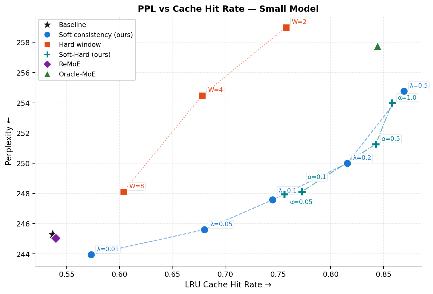

Figure 2: Quality–locality Pareto frontier (cache hit rate vs.perplexity) on WikiText-2 for small and medium models. Each point represents one method configuration; higher cache hit rate and lower perplexity are both desirable (upper-left is better). StickyMoE Soft and Soft-Hard variants trace a smooth Pareto frontier, consistently achieving higher cache hit rates at comparable or better perplexity than the Hard baseline, ReMoE, and Oracle-MoE. ReMoE fails to meaningfully improve cache hit rate at either scale, clustering near the Baseline point.. a — Small model (\({\sim}\)8.8M params), b — Medium model (\({\sim}\)22M params)
Figure 2 illustrates the quality–locality Pareto frontier. StickyMoE Soft and Soft-Hard variants strictly dominate ReMoE across all operating points: because ReMoE fails to move SR meaningfully, it offers no cache efficiency benefit whatsoever despite the additional fine-tuning cost. Oracle-MoE achieves competitive locality but requires architectural changes to the router input; StickyMoE matches or exceeds its cache hit rate without any structural modification. The Hard baseline traces a separate, dominated frontier — high locality is achievable but only at perplexity costs that make the model uncompetitive.
The cache impact is directly quantified by our LRU simulations (\(C{=}2\) expert slots). On the small model, StickyMoE at \(\lambda{=}0.1\) reduces SR from \(0.71\) to \(0.47\), raising CHR from \(0.54\) to \(0.75\) — a \(1.82\times\) reduction in cache misses. The effect is more pronounced on the medium model: at \(\lambda{=}0.5\), SR drops from \(0.71\) to \(0.29\), raising CHR from \(0.54\) to \(0.88\) — a \(3.92\times\) reduction in cache misses, translating directly into lower per-token latency on bandwidth-limited edge hardware.
5.8 Ablation Studies↩︎
| Method | L0 \(\downarrow\) | L1 \(\downarrow\) | L2 \(\downarrow\) | L3 \(\downarrow\) | ||||||||||||||||||||||||||||||||||||||||||||||||||||||||||||||||||||||||
|---|---|---|---|---|---|---|---|---|---|---|---|---|---|---|---|---|---|---|---|---|---|---|---|---|---|---|---|---|---|---|---|---|---|---|---|---|---|---|---|---|---|---|---|---|---|---|---|---|---|---|---|---|---|---|---|---|---|---|---|---|---|---|---|---|---|---|---|---|---|---|---|---|---|---|---|---|
| Baseline | 0.732 | 0.739 | 0.733 | 0.646 | ||||||||||||||||||||||||||||||||||||||||||||||||||||||||||||||||||||||||
| Soft (\(\lambda=0.01\)) | 0.722 | 0.717 | 0.660 | 0.619 | ||||||||||||||||||||||||||||||||||||||||||||||||||||||||||||||||||||||||
| Soft (\(\lambda=0.05\)) | 0.674 | 0.577 | 0.557 | 0.346 | ||||||||||||||||||||||||||||||||||||||||||||||||||||||||||||||||||||||||
| Soft (\(\lambda=0.10\)) | 0.642 | 0.423 | 0.367 | 0.299 | ||||||||||||||||||||||||||||||||||||||||||||||||||||||||||||||||||||||||
| Soft (\(\lambda=0.20\)) | 0.617 | 0.317 | 0.291 | 0.245 | ||||||||||||||||||||||||||||||||||||||||||||||||||||||||||||||||||||||||
| Soft (\(\lambda=0.50\)) | 0.549 | 0.177 | 0.232 | 0.205 | ||||||||||||||||||||||||||||||||||||||||||||||||||||||||||||||||||||||||
| Hard (\(W=2\)) | 0.519 | 0.462 | 0.417 | 0.492 | ||||||||||||||||||||||||||||||||||||||||||||||||||||||||||||||||||||||||
| Hard (\(W=4\)) | 0.621 | 0.683 | 0.602 | 0.557 | ||||||||||||||||||||||||||||||||||||||||||||||||||||||||||||||||||||||||
| Hard (\(W=8\)) | 0.707 | 0.716 | 0.714 | 0.593 | ||||||||||||||||||||||||||||||||||||||||||||||||||||||||||||||||||||||||
| Soft-Hard (\(\lambda=0.1\), \(\alpha=0.05\), \(W=4\)) | 0.638 | 0.390 | 0.378 | 0.245 | ||||||||||||||||||||||||||||||||||||||||||||||||||||||||||||||||||||||||
| Soft-Hard (\(\lambda=0.1\), \(\alpha=0.10\), \(W=4\)) | 0.637 | 0.326 | 0.324 | 0.279 | ||||||||||||||||||||||||||||||||||||||||||||||||||||||||||||||||||||||||
| Soft-Hard (\(\lambda=0.1\), \(\alpha=0.50\), \(W=4\)) | 0.620 | 0.181 | 0.299 | 0.197 | ||||||||||||||||||||||||||||||||||||||||||||||||||||||||||||||||||||||||
| Soft-Hard (\(\lambda=0.1\), \(\alpha=1.00\), \(W=4\)) | 0.576 | 0.108 | 0.215 | 0.196 | ||||||||||||||||||||||||||||||||||||||||||||||||||||||||||||||||||||||||
| ReMoE (\(\lambda=0.1\)) | 0.731 | 0.737 | 0.733 | 0.636 | ||||||||||||||||||||||||||||||||||||||||||||||||||||||||||||||||||||||||
| Oracle-MoE | 0.513 | 0.166 | 0.306 | 0.280 |
10pt
5.8.0.1 Per-layer consistency profiles.
Tables 9 and 8 show per-layer switch rates across all methods. Two consistent patterns emerge across both model sizes. First, L0 is the most resistant layer: even at \(\lambda{=}0.5\), L0 SR remains above \(0.49\) on both models, compared to reductions to \(0.22\) and below at L1–L3. This is expected — L0 processes token embeddings before any contextual mixing via attention, making adjacent tokens intrinsically more dissimilar at that layer. Second, the consistency loss distributes its effect non-uniformly: L1 and L2 see the largest absolute reductions, suggesting these layers are most amenable to locality regularisation once some contextual integration has occurred. The Soft-Hard variant at \(\alpha{=}1.0\) achieves the single lowest per-layer SR in either table: L1 \(= 0.108\) on the medium model, an \(85\%\) reduction from the Baseline value of \(0.739\).
5.8.0.2 \(\lambda\) sensitivity.
The medium model is substantially more robust to large \(\lambda\) than the small model. On the small model, \(\lambda{=}0.5\) incurs \(+3.9\%\) PPL; on the medium model the same \(\lambda\) incurs only \(-0.9\%\) (an improvement). This scaling behaviour is encouraging: as model capacity grows, the consistency constraint becomes easier to satisfy without sacrificing representational quality, suggesting StickyMoE will become more effective, not less, at larger scales.
6 Discussion↩︎
6.0.0.1 When does StickyMoE help most?
The consistency loss is most beneficial when two conditions hold simultaneously: the target hardware has severely constrained fast memory relative to expert size, making each cache miss expensive, and the target domain has natural local coherence — long-form text, code, conversations, documents — that the consistency loss can reinforce. Our results suggest a third condition that was not anticipated: StickyMoE is more effective at larger model scales. On the medium model, moderate \(\lambda\) values actually improve perplexity relative to the baseline, suggesting that larger expert networks have sufficient capacity to satisfy the routing constraint without sacrificing representational quality. This is an encouraging sign for deployment at scale.
6.0.0.2 Why post-hoc fine-tuning fails.
The most striking empirical finding is the complete ineffectiveness of ReMoE-style post-hoc router fine-tuning. Across both model sizes and all four layers, ReMoE produces switch rates within \(0.5\%\) of the Baseline — a negligible change despite additional compute. This is not a failure of the fine-tuning procedure itself but a fundamental consequence of the representation mismatch problem: the expert weight matrices were trained without any locality incentive, and the hidden representations they produce do not cluster in a way that supports temporally stable routing. Fine-tuning only the router cannot overcome this because the router’s input space is fixed. StickyMoE avoids this by shaping both representations and routing decisions jointly from the first training step.
6.0.0.3 The L0 barrier.
Across all methods and both model sizes, layer L0 is consistently the most resistant to locality improvement. Even at \(\lambda{=}0.5\), L0 switch rate remains above \(0.49\), while L1–L3 drop to \(0.17\)–\(0.24\). We attribute this to the nature of L0 inputs: token embeddings carry token-specific identity information and have not yet been mixed with contextual information via attention. Adjacent tokens are therefore genuinely dissimilar at L0 in a way that the consistency loss cannot easily overcome without large perplexity cost. This suggests that future work targeting L0 specifically — perhaps through embedding-level smoothing or subword-aware routing — could yield further locality gains.
6.0.0.4 Relationship to language structure.
The non-uniform distribution of locality gains across layers is consistent with the view that higher layers represent more abstract, semantically stable information while lower layers process surface-level token features. StickyMoE effectively asks lower layers to behave more like higher layers from a routing perspective. The fact that this is achievable at moderate \(\lambda\) without quality loss suggests that the routing surface in these layers is more flexible than the representations themselves — the router can be steered toward consistency without the underlying features needing to change dramatically. Consistent with this, L1 SR drops from \(0.739\) to \(0.177\) at \(\lambda{=}0.5\) on the medium model while PPL simultaneously improves by \(0.9\%\) — evidence that the routing surface at L1 is genuinely more flexible than the representations it operates on.
6.0.0.5 Towards cross-layer routing consistency.
The consistency loss proposed in this paper operates within each layer across consecutive tokens, which is most directly beneficial during prefill and batched decode. For single-token autoregressive decoding — the dominant inference mode on memory-constrained edge devices — the forward pass traverses all layers sequentially for each token, making cross-layer memory access the primary bottleneck. A complementary cross-layer consistency loss that encourages the same expert to be selected at consecutive layers for the same token would directly target this bottleneck. However, such a loss only reduces cache misses if expert weights are shared across layers, since routing consistently to expert \(i\) at layers \(\ell\) and \(\ell+1\) only avoids a memory load when \(\mathcal{E}_i^{(\ell)} = \mathcal{E}_i^{(\ell+1)}\). In standard MoE models with independent per-layer expert matrices, cross-layer routing consistency provides no cache benefit. We provide a full analysis of this access pattern, the parameter sharing requirement, and a proposed combined training objective in 11.
6.0.0.6 Limitations.
The consistency loss penalises switches uniformly regardless of whether a switch occurs at a natural semantic boundary — a sentence break, topic shift, or dialogue turn — or in the middle of a coherent span. At a sentence boundary, switching experts is semantically appropriate and penalising it unnecessarily constrains the model. A boundary-aware variant that gates the consistency loss using punctuation or BOS signals would relax the penalty precisely where switching is warranted and strengthen it where it is not. We expect this would improve the quality–locality trade-off particularly at higher \(\lambda\) values where the current formulation begins to hurt perplexity. We leave this to future work.
7 Conclusion↩︎
We introduced StickyMoE, a training-time routing consistency loss for Mixture-of-Experts language models that directly optimises for temporal locality in expert activation patterns. By penalising abrupt expert switches between adjacent tokens during pretraining, StickyMoE produces routers that are intrinsically locality-aware without requiring any architectural modifications or post-hoc adaptation. Experiments on small and medium MoE models demonstrate that StickyMoE reduces the expert switch rate by up to 59% while simultaneously improving perplexity on the medium model, and reduces cache misses by up to \(\mathbf{3.92\times}\) — a result that stands in stark contrast to post-hoc router fine-tuning, which fails to meaningfully reduce switch rate at either scale, confirming that routing locality cannot be retrofitted and must be instilled during training.
These results instantiate a broader principle: inference-time memory access patterns are a legitimate training objective. Just as quantisation-aware training [23] has become standard practice by demonstrating that training with deployment constraints in the loop consistently outperforms post-hoc compression, we argue that locality-aware training should be the default starting point for MoE models intended for memory-constrained deployment. The post-hoc stack — caching heuristics, router fine-tuning, offloading schedulers — remains useful as a complement, but not as a substitute for a model that was never asked to be cache-friendly in the first place.
7.0.0.1 Future work.
Promising directions include: scaling StickyMoE to larger MoE models (1B+ parameters) where the regularisation benefit observed at medium scale may be even more pronounced; boundary-aware consistency losses that relax the penalty at sentence and paragraph boundaries; combining StickyMoE with structured expert grouping so that switches within a group are cheaper than switches across groups; and investigating whether experts trained with StickyMoE develop more interpretable and topically coherent specialisations, given that they process longer contiguous spans of semantically related tokens — a testable prediction that consistent routing implies more coherent and persistent expert assignments across a document.
8 Reproducibility↩︎
All code, configuration files, and dependency versions are committed to the project repository. Exact package versions are specified in uv.lock. The WikiText-2 dataset is downloaded from the HuggingFace Hub
(Salesforce/wikitext, split wikitext-2-raw-v1) and cached locally as NumPy arrays. The full experiment pipeline is reproducible by running:
    uv sync
    uv run python download_data.py
    bash run_experiments.sh
9 Switch Rate Pareto Frontier↩︎
Figure 3 shows the quality–locality Pareto frontier using switch rate as the locality metric, complementing the cache hit rate frontier in the main text.
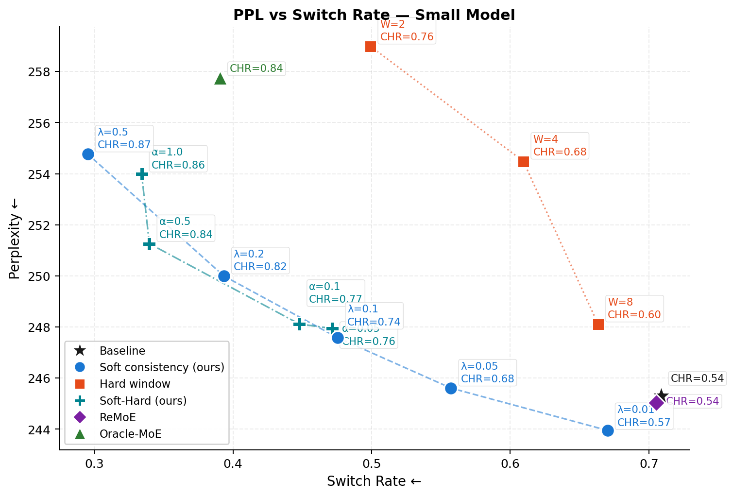
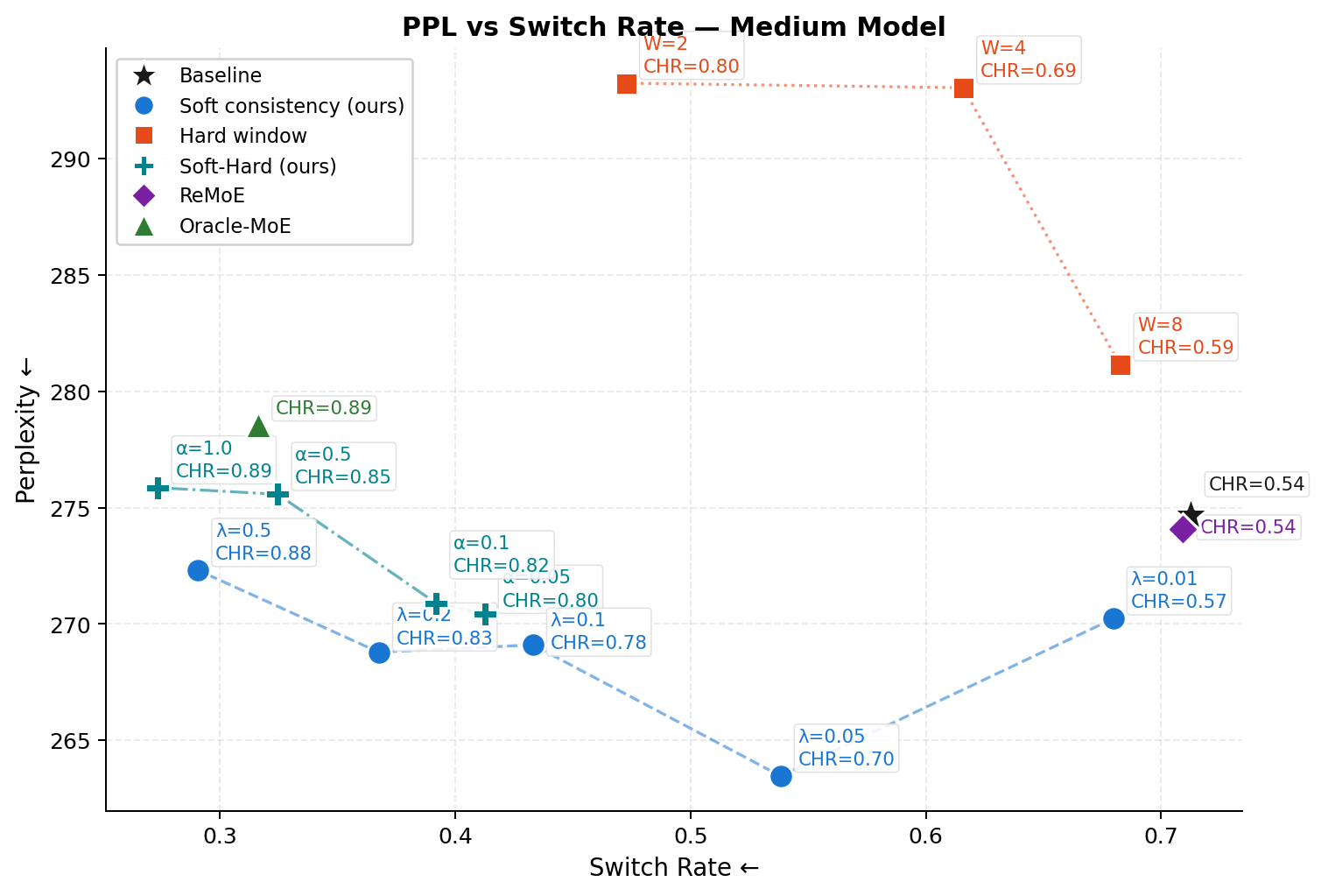
Figure 3: Quality–locality Pareto frontier (switch rate vs.perplexity) on WikiText-2 for small and medium models. Each point represents one method configuration; lower switch rate and lower perplexity are both desirable (lower-left is better). StickyMoE Soft and Soft-Hard variants trace a smooth Pareto frontier, consistently achieving lower switch rates at comparable or better perplexity than the Hard baseline, ReMoE, and Oracle-MoE. ReMoE fails to meaningfully reduce switch rate at either scale, clustering near the Baseline point.. a — Small model (\({\sim}\)8.8M params), b — Medium model (\({\sim}\)22M params)
10 Per-Layer Switch Rates: Small Model↩︎
| Method | L0 \(\downarrow\) | L1 \(\downarrow\) | L2 \(\downarrow\) | L3 \(\downarrow\) | ||||||||||||||||||||||||||||||||||||||||||||||||||||||||||||||||||||||||
|---|---|---|---|---|---|---|---|---|---|---|---|---|---|---|---|---|---|---|---|---|---|---|---|---|---|---|---|---|---|---|---|---|---|---|---|---|---|---|---|---|---|---|---|---|---|---|---|---|---|---|---|---|---|---|---|---|---|---|---|---|---|---|---|---|---|---|---|---|---|---|---|---|---|---|---|---|
| Baseline | 0.716 | 0.714 | 0.715 | 0.691 | ||||||||||||||||||||||||||||||||||||||||||||||||||||||||||||||||||||||||
| Soft (\(\lambda=0.01\)) | 0.680 | 0.684 | 0.681 | 0.636 | ||||||||||||||||||||||||||||||||||||||||||||||||||||||||||||||||||||||||
| Soft (\(\lambda=0.05\)) | 0.653 | 0.597 | 0.459 | 0.520 | ||||||||||||||||||||||||||||||||||||||||||||||||||||||||||||||||||||||||
| Soft (\(\lambda=0.10\)) | 0.641 | 0.546 | 0.326 | 0.389 | ||||||||||||||||||||||||||||||||||||||||||||||||||||||||||||||||||||||||
| Soft (\(\lambda=0.20\)) | 0.571 | 0.428 | 0.304 | 0.271 | ||||||||||||||||||||||||||||||||||||||||||||||||||||||||||||||||||||||||
| Soft (\(\lambda=0.50\)) | 0.488 | 0.234 | 0.220 | 0.239 | ||||||||||||||||||||||||||||||||||||||||||||||||||||||||||||||||||||||||
| Hard (\(W=2\)) | 0.563 | 0.538 | 0.531 | 0.363 | ||||||||||||||||||||||||||||||||||||||||||||||||||||||||||||||||||||||||
| Hard (\(W=4\)) | 0.628 | 0.679 | 0.600 | 0.531 | ||||||||||||||||||||||||||||||||||||||||||||||||||||||||||||||||||||||||
| Hard (\(W=8\)) | 0.670 | 0.729 | 0.676 | 0.578 | ||||||||||||||||||||||||||||||||||||||||||||||||||||||||||||||||||||||||
| Soft-Hard (\(\lambda=0.1\), \(\alpha=0.05\), \(W=4\)) | 0.647 | 0.532 | 0.327 | 0.380 | ||||||||||||||||||||||||||||||||||||||||||||||||||||||||||||||||||||||||
| Soft-Hard (\(\lambda=0.1\), \(\alpha=0.10\), \(W=4\)) | 0.622 | 0.521 | 0.325 | 0.324 | ||||||||||||||||||||||||||||||||||||||||||||||||||||||||||||||||||||||||
| Soft-Hard (\(\lambda=0.1\), \(\alpha=0.50\), \(W=4\)) | 0.600 | 0.281 | 0.270 | 0.208 | ||||||||||||||||||||||||||||||||||||||||||||||||||||||||||||||||||||||||
| Soft-Hard (\(\lambda=0.1\), \(\alpha=1.00\), \(W=4\)) | 0.585 | 0.264 | 0.235 | 0.252 | ||||||||||||||||||||||||||||||||||||||||||||||||||||||||||||||||||||||||
| ReMoE (\(\lambda=0.1\)) | 0.715 | 0.712 | 0.711 | 0.684 | ||||||||||||||||||||||||||||||||||||||||||||||||||||||||||||||||||||||||
| Oracle-MoE | 0.676 | 0.229 | 0.290 | 0.367 |
10pt
11 Cross-Layer Routing Consistency: A Forward-Looking Analysis↩︎
11.1 The Decode-Time Memory Access Pattern↩︎
The consistency loss proposed in the main paper operates within a layer across consecutive tokens: \[\mathcal{L}_{\text{cons}}^{(\ell)} = \frac{1}{T-1}\sum_{t=2}^{T} \bigl\| \mathbf{g}_t^{(\ell)} - \mathbf{g}_{t-1}^{(\ell)} \bigr\|_2^2.\] This formulation is well-motivated for prefill (where many tokens are processed in parallel, one layer at a time) and for batched decode. For single-token autoregressive decoding — the dominant inference mode on memory-constrained edge devices — the memory access pattern is different. The forward pass processes one token at a time and traverses all layers sequentially: \[\text{token } t: \quad \mathcal{E}^{(0)} \;\to\; \mathcal{E}^{(1)} \;\to\; \mathcal{E}^{(2)} \;\to\; \cdots \;\to\; \mathcal{E}^{(L-1)},\] so consecutive memory accesses are across layers for the same token, not across tokens for the same layer. The access sequence for two consecutive tokens under single-token decode is:
| Step | Token | Expert loaded |
|---|---|---|
| 1 | \(t\) | \(\mathcal{E}^{(0)}_{\sigma_t^{(0)}}\) |
| 2 | \(t\) | \(\mathcal{E}^{(1)}_{\sigma_t^{(1)}}\) |
| 3 | \(t\) | \(\mathcal{E}^{(2)}_{\sigma_t^{(2)}}\) |
| 4 | \(t\) | \(\mathcal{E}^{(3)}_{\sigma_t^{(3)}}\) |
| 5 | \(t+1\) | \(\mathcal{E}^{(0)}_{\sigma_{t+1}^{(0)}}\) |
| 6 | \(t+1\) | \(\mathcal{E}^{(1)}_{\sigma_{t+1}^{(1)}}\) |
| \(\vdots\) | \(\vdots\) | \(\vdots\) |
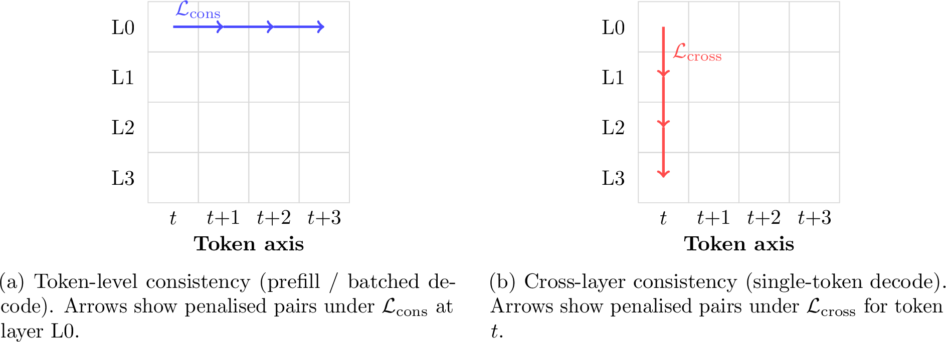
where \(\sigma_t^{(\ell)}\) denotes the expert index selected for token \(t\) at layer \(\ell\). Each step requires loading a potentially different expert weight matrix. Under this access pattern, the token-level consistency loss reduces misses at step 5 relative to step 1 (same layer, adjacent tokens) but does nothing to reduce misses at step 2 relative to step 1 (adjacent layers, same token).
11.2 Cross-Layer Consistency and the Parameter Sharing Requirement↩︎
A natural extension is a cross-layer consistency loss that encourages the same expert to be selected at consecutive layers for the same token: \[\mathcal{L}_{\text{cross}} = \frac{1}{T}\sum_{t=1}^{T}\sum_{\ell=1}^{L-1} \bigl\| \mathbf{g}_t^{(\ell)} - \mathbf{g}_t^{(\ell+1)} \bigr\|_2^2. \label{eq:cross95loss}\tag{15}\] However, there is a critical prerequisite: cross-layer routing consistency only reduces cache misses if the same expert index at different layers refers to the same weight tensor in memory. In a standard MoE model where each layer maintains its own independent set of expert matrices \(\{\mathcal{E}_i^{(\ell)}\}_{i=1}^{N}\), expert 2 at layer \(\ell\) and expert 2 at layer \(\ell+1\) are entirely different weight tensors. Routing consistently to expert 2 across both layers still requires two separate memory loads — no cache benefit is obtained.
Cross-layer consistency therefore becomes practically useful only under one of the following architectural conditions:
Full cross-layer weight sharing. Expert \(i\) is the same weight matrix at every layer: \(\mathcal{E}_i^{(\ell)} = \mathcal{E}_i\) for all \(\ell\). Consistent routing to expert \(i\) across all layers requires only a single load, amortised over \(L\) layers of computation.
Grouped weight sharing. Layers are partitioned into blocks of size \(K\) (e.g. \(K=2\) or \(K=4\)), and all layers within a block share the same expert pool. Consistent routing within a block reduces loads; routing across block boundaries still requires new loads.
Universal expert pool. All layers draw from one shared set of expert matrices — a design explored in recent parameter-efficient architectures. Any cross-layer routing consistency directly translates to cache reuse.
11.3 The Combined Objective↩︎
Under a grouped weight sharing architecture with block size \(K\), the full memory-aware training objective combining token-level and cross-layer consistency would be: \[\mathcal{L}= \mathcal{L}_{\text{CE}} + \lambda\,\mathcal{L}_{\text{cons}} + \mu\,\mathcal{L}_{\text{bal}} + \gamma\,\mathcal{L}_{\text{cross}}, \label{eq:full95loss}\tag{16}\] where \(\gamma \geq 0\) controls the cross-layer consistency weight. The two consistency terms are complementary and target different bottlenecks: \(\mathcal{L}_{\text{cons}}\) reduces misses across tokens at the same layer (prefill and batched decode), while \(\mathcal{L}_{\text{cross}}\) reduces misses across layers for the same token (single-token decode). 4 illustrates the two access patterns and the corresponding consistency objectives.
11.4 Limiting Case: Pre-defined Expert Trajectories↩︎
The consistency objectives proposed in this paper nudge the router toward stable routing decisions but still allow it to adapt freely. A natural limiting case is to remove the router entirely and fix expert assignments before training begins — defining a deterministic trajectory \(\sigma_t = (\sigma_t^{(0)}, \sigma_t^{(1)}, \ldots, \sigma_t^{(L-1)})\) through the network for every token \(t\), where \(\sigma_t^{(\ell)} \in \{1,\ldots,N\}\) is the expert index at layer \(\ell\).
The idea of fixed routing is not new: [24] show that assigning tokens to experts via a deterministic hash function, with no learned router, produces surprisingly competitive models. Our trajectory framing differs in two key respects. First, assignments are coordinated across layers to define a complete network path per token, rather than independent per-layer hashes. Second, trajectories are chosen to maximise cache locality — consecutive tokens are assigned the same trajectory, so the entire sequence of expert weight loads for token \(t\) is identical to that of token \(t{-}1\), yielding zero cache misses within a coherent span.
Under this design the cache miss rate during single-token autoregressive decode is determined entirely by how often the trajectory changes between consecutive tokens — a quantity that is fully under the designer’s control rather than an emergent property of learned routing. In the extreme case where all tokens in a document share the same trajectory, cache misses are eliminated entirely at the cost of routing flexibility. This represents the upper bound on locality achievable by any routing strategy, and serves as a useful reference point for evaluating how close learned consistency objectives like StickyMoE come to the theoretical optimum.
Whether a model trained with fixed locality-maximising trajectories can match the quality of a model with learned routing is an open empirical question. The hash routing results of [24] suggest it is plausible, at least at small to moderate scale. We leave a systematic investigation of this trade-off to future work.
11.5 Implications and Future Work↩︎
The analysis above identifies a gap in the current StickyMoE formulation: it is most directly beneficial for prefill and batched decode, while single-token autoregressive decode — the dominant mode on memory-constrained edge devices — is better served by cross-layer consistency under a parameter-sharing architecture. We leave the empirical validation of \(\mathcal{L}_{\text{cross}}\) and its interaction with grouped weight sharing to future work, noting that the training-time intervention principle extends naturally to this setting: just as token-level locality must be instilled during training rather than retrofitted, cross-layer locality requires architectural choices (parameter sharing) and training objectives (\(\mathcal{L}_{\text{cross}}\)) that are made from the outset.