Guidance Breaks the Fitted Operator:
A Terminal-Fitted Repair for Classifier-Free Guidance
July 08, 2026
Abstract
Classifier-free guidance (CFG) is the standard way to strengthen class-conditioning in diffusion and flow-matching samplers, yet at large guidance it oversaturates and destabilizes—symptoms practitioners suppress with more steps or limited-interval schedules. We analyze CFG through an asymptotic-preserving, numerical-analysis lens. Building on a recent result [1] that the deterministic DDIM step is the unique fitted operator for the unguided terminal layer—exact on the final, small-\(\sigma\) stretch of sampling—we show that guidance re-stiffens exactly the discriminative subspace to an anomalous exponent \(1+w\) (guided coordinates contract like \(\sigma^{1+w}\) rather than \(\sigma\)). DDIM is therefore no longer fitted there, and on coarse meshes its guided residual diverges as \(\sigma_{\min}\to0\). We prove a guided clock barrier with three ordered step-size thresholds, and read one-step oversaturation as its endpoint—a solver artifact on the calibration model rather than the continuous guided law. The same analysis yields a one-coefficient, zero-extra-NFE repair: replace CFG’s \(w(r-1)\) by \(r^{1+w}-r\) on the guidance direction. This coefficient is the unique spectrum-free terminal-exact one, and it preserves the sign of every analyzed coordinate. On the calibration model’s discriminative crossover it removes CFG’s \(\sigma_{\min}\)-divergent blow-up and is first-order accurate against the exact guided flow as \(\sigma_{\min}\to0\)—asymptotic-preserving in \(\sigma_{\min}\), though not uniform in \(w\). On learned CIFAR-10 checkpoints—and, as a cross-domain smoke test, on Stable Diffusion 1.5 DDIM—it acts as a high-guidance stabilizer at no extra cost rather than a universal quality knob: it cuts residual amplification and saturation and gives \(9/9\) point-FID wins over CFG on the tested grid, while in the hard-cell blocks its classifier-proxy target accuracy stays close to CFG and terminal guidance shutdown loses much more. We report the limits alongside: it is not a universal image-quality win (KID can favor CFG; an interval can win FID in some cells), and against a dense vanilla-CFG reference it is not a uniformly better integrator of that field.
1 Introduction↩︎
Diffusion and flow-matching samplers integrate a probability-flow ODE whose velocity field stiffens as the noise scale \(\sigma\to\sigma_{\min}\): on a coordinate normal to the data manifold the exact flow contracts at exponent one, by \(\sigma_{n+1}/\sigma_n\) per step. A recent fitted-operator analysis of unguided samplers [1] shows that this terminal layer admits a unique fitted (layer-exact) one-step operator: a frozen-field Euler step—Euler with the velocity held at its start-of-step value—reproduces that exact contraction if and only if its integration variable is affine in \(\sigma\). This singles out the \(\sigma\)-clock step, algebraically identical to deterministic DDIM [2], and makes it asymptotic-preserving (AP) on the exactly solvable calibration models studied there [1]—uniformly accurate as \(\sigma_{\min}\to0\). This paper asks one question of that lens: what survives of DDIM’s fitted-operator protection once we turn on guidance?
1.0.0.1 Guidance re-stiffens the discriminative subspace.
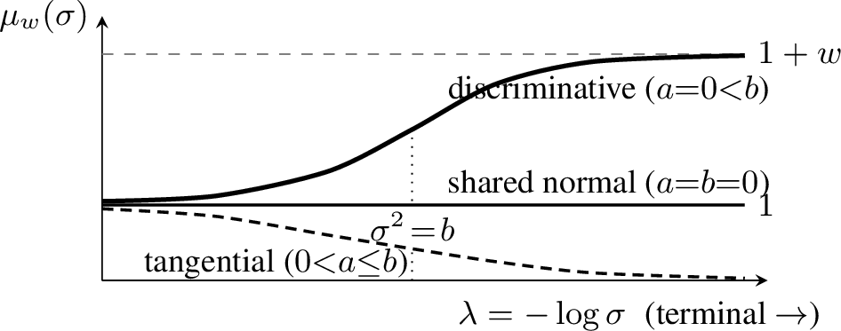
Classifier-free guidance (CFG) [3] runs the sampler on an extrapolated denoiser \(D_{w}=(1+w)D_{\mathrm{c}}-wD_{\mathrm{u}}\), that is, on a second velocity field \(\eta_{w}=\eta_{\mathrm{c}}+w(\eta_{\mathrm{c}}-\eta_{\mathrm{u}})\) (the \(\eta\)’s are noise-prediction fields; Section 2) with guidance scale \(g=1+w\). This is not a uniform stiffening. On the commuting Gaussian model of Section 2, the guided terminal exponent \(\mu_w(\sigma)\) splits by layer (a layer here is a regime of state-space directions, not a network layer; Figure 1): it stays exactly one on directions shared by the class and the marginal, freezes to zero on tangential directions, and rises to \(1+w\) on the discriminative directions—the subspace that separates the class from the marginal (Proposition 1). Guidance re-stiffens precisely this discriminative subspace, and it does so with a second singular parameter: \(w\) enters the terminal structure on the same footing as \(\sigma_{\min}\). Because \(D_{w}\) is not any distribution’s posterior mean, DDIM’s fitted-operator protection lapses there: on coarse meshes, vanilla DDIM\(+\)CFG leaves the class of fitted operators and its terminal residual diverges as \(\sigma_{\min}\to0\).
1.0.0.2 Two orthogonal bills.
This is a statement about the solver. A parallel line studies how the continuous guided law itself departs from the tilted conditional it is meant to sample [4], [5]: that charges the model; we charge the discretization—our reference solution is always the exact guided flow’s own pushforward. The two bills are orthogonal, and conflating them has obscured how much of guidance’s terminal pathology—the oversaturation and norm inflation seen at large \(w\) [6]—has a solver-induced component that appears even when the exact guided flow is the reference, from stepping guidance with an operator it has quietly un-fitted.
1.0.0.3 The repair is one coefficient.
Rectifying the anomalous exponent \(1+w\) by a gauge change and pushing the \(\sigma\)-clock step through it yields a one-coefficient modification of CFG that touches nothing else in the sampler—only the coefficient on the guidance direction \(D_{\mathrm{u}}-D_{\mathrm{c}}\) changes: \[\begin{align} \text{CFG:} \quad & x_{n+1}=D_{\mathrm{c}}+r\,(x_n-D_{\mathrm{c}})+w(r-1)\,(D_{\mathrm{u}}-D_{\mathrm{c}}),\\ \text{fitted:} \quad & x_{n+1}=D_{\mathrm{c}}+r\,(x_n-D_{\mathrm{c}})+\bigl(r^{1+w}-r\bigr)(D_{\mathrm{u}}-D_{\mathrm{c}}), \end{align}\] with \(r=\sigma_{n+1}/\sigma_n\). It uses the same two denoiser evaluations per step—the implementation delta is a single line, at zero additional NFE (network function evaluations)—agrees with CFG to first order, and reduces to DDIM at \(w=0\). We call it the guided fitted step, or fitted CFG. It is the unique scalar coefficient that is exact on the discriminative terminal layer using no spectral information (Lemma 2); it never reflects a coordinate across the class manifold (Proposition 3); and its one-step \(r\to0\) limit lands on the conditional denoiser \(D_{\mathrm{c}}\) (the terminal-limit class projection), where vanilla CFG lands on the overshot \(D_{w}\), the discrete mechanism of oversaturation.
1.0.0.4 Contributions.
Structure and a barrier. A layer classification of the guided terminal exponent (Proposition 1) and a guided clock barrier (Theorem 1) with three ordered step-size thresholds—reflection, residual-amplification failure (Section 3), absolute stability—and the resulting two-tier guidance tax on step count (Corollary 1).
Oversaturation as an endpoint, and the guidance interval. A model-free identity reading one-step DDIM\(+\)CFG’s overshoot to \(D_{w}\) as the barrier’s \(r\to0\) endpoint (Remark 2), and a parameter-free prediction of the terminal edge of limited-interval guidance [7] (Remark 3).
A spectrum-free fitted repair. The guided fitted step (Definition 1): first-order consistent, sign-preserving and terminal-exact on the model, unique (Lemma 2), and—on the discriminative crossover—free of the \(\sigma_{\min}\)-divergent blow-up and first-order accurate as \(\sigma_{\min}\to0\) (Proposition 4, Theorem 2): asymptotic-preserving in \(\sigma_{\min}\), though not uniform in \(w\).
A scoped empirical program. On learned CIFAR-10 edm [8] checkpoints, fitted CFG is a zero-extra-NFE high-guidance stabilizer: the residual and clipping certificates improve in both \(w\in\{6.5,8\}\) cells; the hard-cell image evaluations (two 5k blocks, a 50k replication) give it the best FID with target accuracy preserved, and a DINOv2 backbone-swap keeps the same fitted-favoring ordering; a nine-cell grid gives \(9/9\) FID wins over CFG. We report the limits alongside—the CFG-favoring KID split and threshold-derived interval baselines that win FID/KID at lower conditionality (Section 4).
Section 6 collects the claim boundaries.
ifarxiv ifarxiv
2 The guided flow and its terminal layers↩︎
2.0.0.1 The unguided flow.
We work throughout in the variance-exploding family: \(p_\sigma = p_{\rm data} * \mathcal{N}(0,\sigma^2 I)\) for \(\sigma \in [\sigma_{\min},\sigma_{\max}]\), with denoiser \(D(x,\sigma) = \mathbb{E}[x_0 \mid x_\sigma = x]\) and normalized residual \(\eta = (x - D)/\sigma\)—the noise prediction \(\hat{\varepsilon}\) of practice (\(-\sigma\nabla_x \log p_\sigma\)); not DDIM’s stochasticity parameter, which is \(0\) throughout. The probability flow ODE is \(\mathrm{d}X/\mathrm{d}\sigma = \eta(X,\sigma)\), and the decomposition \(x = D + \sigma\eta\) splits the state into a slow manifold component and a stiff normal component—normal to the data manifold, contracting fastest—whose exponent is \(1\): on a normal coordinate the exact flow contracts by \((\sigma_{n+1}/\sigma_n)^1\) per step. A fitted-operator analysis of the unguided terminal layer [1] shows that a frozen-field Euler step is layer-exact if and only if its clock is affine in \(\sigma\), making the \(\sigma\)-clock step—algebraically the deterministic DDIM update [2]—the unique fitted operator up to affine reparameterization, with rectified flow its flow-matching counterpart; this fitted-operator property is what makes it asymptotic-preserving as \(\sigma_{\min}\to 0\). The present paper asks what survives of that protection under guidance.
2.0.0.2 Guidance as a second velocity field.
Classifier-free guidance [3] replaces the conditional denoiser \(D_{\mathrm{c}}(x,\sigma)\) by the extrapolation \[\label{eq:guided-denoiser} D_{w}\;=\; (1+w)\,D_{\mathrm{c}}\;-\; w\,D_{\mathrm{u}}, \qquad w \ge 0,\tag{1}\] where \(D_{\mathrm{u}}\) is the unconditional (marginal) denoiser and \(g = 1+w\) is the guidance scale of practice, so \(w=6.5\) is CFG scale \(g=7.5\). Writing \(\eta_{\mathrm{c}}= (x-D_{\mathrm{c}})/\sigma\) and \(\eta_{\mathrm{u}}= (x-D_{\mathrm{u}})/\sigma\), the sampled dynamics is the guided flow \[\label{eq:guided-flow} \frac{\mathrm{d}X}{\mathrm{d}\sigma} \;=\; \eta_{w} \;=\; (1+w)\,\eta_{\mathrm{c}}- w\,\eta_{\mathrm{u}} \;=\; \eta_{\mathrm{c}}+ w\,\gamma, \qquad \gamma \;:=\; \eta_{\mathrm{c}}- \eta_{\mathrm{u}}\;=\; \frac{D_{\mathrm{u}}- D_{\mathrm{c}}}{\sigma},\tag{2}\] with \(\gamma\) the normalized guidance direction. Equation (2 ) is the dynamical statement of guidance: the sampler follows the conditional velocity plus \(w\) times the discriminative correction. Two facts follow. First, \(D_{w}\) is in general not a VE posterior mean with a positive-semidefinite Tweedie covariance, so \(\eta_{w}\) is not the residual of such a denoiser; the rigidity theorem that singles out DDIM as layer-exact inside the unguided denoiser class [1] no longer applies directly. The exit is quantitative, not merely definitional: for any true denoiser, \(J_D = \nabla_x D = \mathrm{Cov}(X_0 \mid x)/\sigma^2 \succeq 0\) [9] caps the exponent of the residual field at \(1\) (on the model, the residual exponent is \(A \le 1\) in (3 )), while on discriminative directions the guided exponent exceeds \(1\) at every \(\sigma\) (Proposition 1)—no repackaging of any denoiser, affine or otherwise, reproduces the guided field. Second, the guided flow carries a second parameter: any AP statement must state its \(w\)-dependence, and the fitted step below removes the \(\sigma_{\min}\)-divergent terminal barrier for bounded \(w\), though not uniformly in \(w\).
2.0.0.3 The model problem.
Our analysis is carried out on the guided analog of the unguided model problem [1].
Hypothesis 1 (commuting class–marginal pair). \(p_{\mathrm c} = \mathcal{N}(0, C_{\mathrm c})\) and \(p_{\mathrm u} = \mathcal{N}(0, C_{\mathrm u})\) with \([C_{\mathrm c}, C_{\mathrm u}] = 0\), and on the shared eigenbasis the spectra satisfy \(a_i \le b_i\).
The ordering \(a_i \le b_i\) is the class-subset hypothesis: the class is narrower than the marginal in every probed direction (as when the marginal is a mixture whose components share the class covariance). Real learned checkpoints need not obey it; the reverse case is a genuine model boundary, discussed in Remark [rem:reverse]. On an eigen-coordinate \(\xi\) with class variance \(a\) and marginal variance \(b\), the two denoisers are linear and the residuals are \[\label{eq:AB} \eta_{\mathrm{c}}= A\,\frac{\xi}{\sigma}, \qquad \eta_{\mathrm{u}}= B\,\frac{\xi}{\sigma}, \qquad A := \frac{\sigma^2}{a+\sigma^2}, \quad B := \frac{\sigma^2}{b+\sigma^2}, \quad 0 \le B \le A \le 1 .\tag{3}\] The guided flow (2 ) therefore closes coordinate-wise, \[\label{eq:mu} \frac{\mathrm{d}\log \xi}{\mathrm{d}\log \sigma} \;=\; \mu_w(\sigma) \;:=\; (1+w)A - wB \;=\; A + w\,(A - B),\tag{4}\] and every question about clocks, stability, and fitted operators reduces to the behavior of the exponent function \(\mu_w\).
Proposition 1 (layer classification under guidance). Under Hypothesis 1, as \(\sigma \to 0\) the exponent function (4 ) satisfies: (i) on shared normal directions (\(a = b = 0\)), \(\mu_w \equiv 1\): the guidance weight cancels and the layer is the unguided exponent-\(1\) layer; (ii) on tangential directions (\(0 < a \le b\)), \(\mu_w \to 0\): the coordinate freezes; (iii) on discriminative normal* directions (\(a = 0 < b\)), \[\label{eq:crossover} \mu_w(\sigma) \;=\; 1 + w\,\frac{b}{b+\sigma^2} \;\longrightarrow\; 1+w ,\tag{5}\] monotonically as \(\sigma\) decreases, with crossover midpoint at \(\sigma^2 = b\).*
(Proofs for Sections 2 and 3 are deferred to Appendix 7.)
Proposition 1 is the structural fact of the paper. Guidance does not stiffen the flow uniformly; it re-stiffens exactly the discriminative subspace—the directions collapsed within the class but present in the marginal (\(a=0<b\))—and (5 ) locates where the re-stiffening begins: the anomalous exponent switches on as \(\sigma\) descends through the class-separation scale \(\sqrt b\). Above that scale the guided flow is, to leading order, the unguided flow; below it, the terminal layer runs at exponent \(1+w\), and \(w\) enters the singular structure of the problem on the same footing as \(\sigma_{\min}\).
Lemma 1 (exact guided factor). Under Hypothesis 1, the exact solution of (2 ) on an eigen-coordinate over one step \(\sigma_n \to \sigma_{n+1}\) is \(\xi_{n+1} = \Phi_w\,\xi_n\) with \[\label{eq:exact-factor} \Phi_w \;=\; \left(\frac{a+\sigma_{n+1}^2}{a+\sigma_n^2}\right)^{\!\frac{1+w}{2}} \left(\frac{b+\sigma_n^2}{b+\sigma_{n+1}^2}\right)^{\!\frac{w}{2}} .\tag{6}\] In particular, on a discriminative coordinate (\(a=0\)), writing \(r = \sigma_{n+1}/\sigma_n\), \[\label{eq:exact-disc} \Phi_w \;=\; r^{\,1+w} \left(\frac{b+\sigma_n^2}{b+\sigma_{n+1}^2}\right)^{\!\frac{w}{2}},\tag{7}\] which tends to \(r^{1+w}\) once \(\sigma_n^2 \ll b\).
The singular limit now has two knobs. As \(\sigma_{\min}\to 0\) the discriminative layer contracts by the anomalous power \(\sigma^{1+w}\); as \(w\) grows at fixed \(\sigma_{\min}\) the same layer stiffens without bound. We ask two questions: which part of DDIM\(+\)CFG’s failure is the pure terminal-layer solver barrier, and can that barrier be removed by a one-coefficient fitted repair? Uniform accuracy through the finite-\(\sigma\) crossover is separate, needing either mesh resolution of the crossover or the spectrum-aware Gaussian factor.
3 The guided barrier and the fitted operator↩︎
This section establishes one claim: classifier-free guidance introduces a second singular parameter \(w\), and on discriminative terminal directions the \(\sigma\)-clock frozen-field step—DDIM applied to the guided denoiser—is no longer fitted. The program has three parts. First, a barrier: the guided analog of the unguided clock dichotomy [1], with sharp thresholds in the log-step \(h\) and weight \(w\) (Theorem 1). Second, an operator: a fitted step that removes the pure discriminative terminal-layer reflection and \(\sigma_{\min}\)-divergent residual blow-up at zero additional cost (Definition 1). Third, accuracy: a first-order certificate on the discriminative crossover (Theorem 2); the whole-model theory remains future work. Throughout, the reference solution is the exact guided flow’s own pushforward: we charge the discretization of (2 ), not the distortion of the continuous guided law away from the tilted conditional (Section 1).
3.0.0.1 The frozen step.
DDIM applied to \(D_{w}\)—equivalently, \(\sigma\)-clock Euler with the guided field frozen at the left endpoint—is \[\label{eq:cfg-step} x_{n+1} \;=\; x_n + (\sigma_{n+1}-\sigma_n)\,\eta_{w}(x_n,\sigma_n),\tag{8}\] which on an eigen-coordinate of the model contracts by \[\label{eq:Gcfg} G_{\rm CFG} \;=\; 1 - (1-r)\bigl[(1+w)A - wB\bigr], \qquad r = \frac{\sigma_{n+1}}{\sigma_n} = \mathrm{e}^{-h}.\tag{9}\] On the pure discriminative layer \((A,B)=(1,0)\) this is \[\label{eq:Gw} G_w(h) \;=\; 1 - (1+w)\,(1-\mathrm{e}^{-h}) \;=\; (1+w)\,\mathrm{e}^{-h} - w ,\tag{10}\] to be compared with the exact factor \(\mathrm{e}^{-(1+w)h}\) of Lemma 1. Here \(h = \log(\sigma_n/\sigma_{n+1})\) is the step in \(\lambda = -\log\sigma\) (half the VE log-SNR), so a uniform \(\lambda\)-mesh has constant \(h\). Along a trajectory, call \(\max_n \|\eta_{w}(x_n,\sigma_n)\|/\|\eta_{w}(x_0,\sigma_0)\|\) the residual-amplification certificate, written \(\mathrm{amp}\); the sampler already forms every quantity in it, and a scheme is residual-stable if the certificate stays bounded as \(\sigma_{\min}\to 0\). Everything in Theorem 1 is a statement about the elementary function (10 ).
Theorem 1 (guided clock barrier). Consider the frozen step (8 ) on the pure discriminative layer, \(\eta_{w}= (1+w)\,\xi/\sigma\) with \(w > 0\), on a uniform \(\lambda\)-mesh of step \(h\). Let \[\label{eq:thresholds} h_\flat \;=\; \log\!\Bigl(1+\tfrac1w\Bigr), \qquad h_\sharp \;=\; \log\!\Bigl(1+\tfrac2w\Bigr), \qquad h_\infty \;=\; \log\!\Bigl(\tfrac{1+w}{\,w-1\,}\Bigr)\;(w>1).\tag{11}\] Then \(h_\flat < h_\sharp < h_\infty\), and:
Sign. \(G_w(h) > 0\) iff \(h < h_\flat\); equivalently, at fixed \(h\), sign preservation fails once \(w > 1/(\mathrm{e}^{h}-1)\). For \(h > h_\flat\) every step reflects the coordinate across the class manifold.
Residual amplification. The per-step residual amplification is \(|G_w(h)|\,\mathrm{e}^{h}\), which is \(\le 1\) iff \(h \le h_\sharp\); equivalently, raw amplification begins once \(w > 2/(\mathrm{e}^{h}-1)\). For \(h > h_\sharp\) the amplification factor is \(w\mathrm{e}^{h} - (1+w) > 1\) per step. On a terminal subwindow \(\sigma \in [\sigma_{\min}, \varepsilon\sqrt b\,]\), where \(B \le \varepsilon^2/(1+\varepsilon^2)\) makes the exact per-step factor pure-layer up to \(O(\varepsilon^2)\), of \(\lambda\)-length \(\Lambda_\varepsilon = \log(\varepsilon\sqrt b/\sigma_{\min})\) the guided residual grows by \[\label{eq:blowup} \bigl(w\mathrm{e}^{h}-(1+w)\bigr)^{\Lambda_\varepsilon/h} \;=\; \Bigl(\frac{\varepsilon\sqrt b}{\sigma_{\min}}\Bigr)^{\!\rho}, \qquad \rho = \frac{\log\bigl(w\mathrm{e}^{h}-(1+w)\bigr)}{h} > 0 ,\tag{12}\] so for fixed \(\varepsilon>0\) and \(h > h_\sharp\) the scheme fails the amplification certificate as \(\sigma_{\min}\to 0\).
Absolute stability. \(|G_w(h)| \le 1\) for all \(h\) when \(w \le 1\); for \(w > 1\), iff \(h \le h_\infty\).
All three thresholds decay like \(c/w\) as \(w \to \infty\), with \(c = 1, 2, 2\) respectively.
In words: sign preservation fails first (a, above \(h_\flat\): every step reflects across the class manifold), the certificate second (b, above \(h_\sharp\): the residual compounds, diverging as \(\sigma_{\min}\to0\)), absolute stability last (c, only for \(w>1\)).
Corollary 1 (two-tier guidance tax). On a uniform \(\lambda\)-mesh covering the discriminative window (of \(\lambda\)-length \(\Lambda_b = \log(\sqrt b/\sigma_{\min})\)), avoiding reflection requires \[\label{eq:tax} N \;\ge\; \frac{\Lambda_b}{\log(1+1/w)} \;\sim\; w\,\Lambda_b ,\tag{13}\] while merely keeping the residual nonexpansive requires \(N \ge \Lambda_b/\log(1+2/w) \sim \tfrac{w}{2}\Lambda_b\). A uniform global mesh must meet this bound throughout the window, so \(\Lambda_b\) is replaced by the full horizon \(\Lambda=\log(\sigma_{\max}/\sigma_{\min})\): at working scale \(g = 7.5\) (\(\Lambda = \log(80/0.002) \approx 10.6\)), reflection-free sampling already demands \(N \gtrsim 74\) steps—an order of magnitude above unguided-DDIM-accurate budgets [8].
Remark 1 (the reflecting window). In the window \(h \in (h_\flat, h_\sharp]\) the scheme is reflecting but nonexpansive: the flip does not grow the residual. The flip is the mechanism of visible artifacts—the iterate lands on the wrong side of the class manifold each step—while the amplification crossing at \(h_\sharp\) is where the certificate, and any uniform accuracy claim, actually fails. Practitioners tune \(w\) down at low \(\sigma\) well before the certificate diverges: part (a), not part (b), is the threshold their tuning discovers.
Remark 2 (the one-jump limit is oversaturation). The following identity is model-free. A single frozen step (8 ) from \(\sigma_n\) to \(\sigma_{n+1} = r\sigma_n\) with \(r \to 0\) gives \[\label{eq:onejump} x_{n+1} \;\to\; x_n - \sigma_n\,\eta_{w}(x_n,\sigma_n) \;=\; (1+w)\,D_{\mathrm{c}}- w\,D_{\mathrm{u}}\;=\; D_{w}(x_n,\sigma_n):\tag{14}\] one-step DDIM\(+\)CFG lands on the extrapolated denoiser, displaced from the class manifold by \(-w(D_{\mathrm{u}}-D_{\mathrm{c}})\). On the model this is the reflection \(\xi \mapsto -w\,\xi\) of Theorem 1(a) pushed to its endpoint. We read this as the discrete mechanism of the oversaturation and norm-inflation phenomenology reported for large guidance scales [6]: it is a property of the solver at coarse steps, not of the continuous guided flow—on the calibration model the exact flow contracts to \(D_{\mathrm{c}}\) as \(r^{1+w}\) while the frozen step overshoots to \(D_{w}\).
3.0.0.2 The guided fitted step.
The repair is dictated by the same logic that produced DDIM in the unguided setting [1]: integrate the stiff layer exactly and freeze what is slow. The gauge \(\tilde{\xi} = \sigma^{-w}\xi\) rectifies the anomalous exponent \(1+w\) to exponent \(1\); transporting the \(\sigma\)-clock Euler step through the gauge and back yields, on the whole state,
Definition 1 (guided fitted step). With \(r = \sigma_{n+1}/\sigma_n\) and all fields evaluated at \((x_n,\sigma_n)\), \[\label{eq:g2-denoiser} x_{n+1} \;=\; D_{\mathrm{c}}\;+\; r\,\bigl(x_n - D_{\mathrm{c}}\bigr) \;+\; \bigl(r^{\,1+w} - r\bigr)\,\bigl(D_{\mathrm{u}}- D_{\mathrm{c}}\bigr) .\tag{15}\] equivalently, in residual form, \[\label{eq:g2-residual} x_{n+1} \;=\; x_n + (\sigma_{n+1}-\sigma_n)\,\eta_{\mathrm{c}} \;+\; \sigma_n\,\bigl(r^{\,1+w}-r\bigr)\,\gamma .\tag{16}\]
The scheme touches exactly one coefficient of classifier-free guidance: vanilla DDIM\(+\)CFG is (15 ) with the coefficient \(w(r-1)\) in place of \(r^{1+w}-r\) on the guidance direction \(D_{\mathrm{u}}- D_{\mathrm{c}}\). It uses the same two denoiser evaluations per step, so the cost—and the implementation delta—is one line. Proposition 3 verifies the factor coordinate-wise; Lemma 2 pins the coefficient from terminal exactness alone.
Proposition 2 (consistency). \(r^{1+w} - r = w(r-1) + \tfrac12 w(w+1)\,h^2 + O(h^3)\) as \(h \to 0\), so (15 ) is a first-order-consistent discretization of the guided flow (2 ), agreeing with DDIM\(+\)CFG through \(O(h)\); and at \(w = 0\) both coefficients vanish identically, collapsing the scheme to DDIM.
Proposition 3 (the fitted step is sign-preserving and terminal-exact). Under Hypothesis 1, the step (15 ) contracts an eigen-coordinate by \[\label{eq:gfit-decomp} G_{\rm fit} \;=\; 1 - (1-r)A + \bigl(r^{1+w}-r\bigr)(A-B) \;=\; (1-A) \;+\; r\,B \;+\; r^{\,1+w}\,(A-B) ,\qquad{(1)}\] a sum of nonnegative terms; hence \(G_{\rm fit} > 0\) on every coordinate, for every mesh, and every \(w \ge 0\): the fitted step preserves the sign of every analyzed coordinate. It is exact in the three terminal regimes—\(G_{\rm fit} = r\) on shared normals \((A=B=1)\), \(G_{\rm fit} = r^{1+w}\) on pure discriminative normals \((A=1, B=0)\), and \(G_{\rm fit} = 1\) on frozen tangential directions \((A=B=0)\)—and its one-jump limit is \(x_{n+1} \to D_{\mathrm{c}}\), the conditional denoiser (the terminal-limit class projection), in contrast with (14 ).
Lemma 2 (uniqueness of the scalar terminal coefficient). Consider scalar coefficient updates of the form \[x_{n+1} = D_{\mathrm{c}}+ r(x_n-D_{\mathrm{c}}) + \alpha(r,w)(D_{\mathrm{u}}-D_{\mathrm{c}}),\] where \(\alpha\) depends only on \((r,w)\). The unique such coefficient that is exact on the pure discriminative terminal regime \((A,B)=(1,0)\) is \[\alpha(r,w) = r^{1+w}-r .\] Consequently, terminal exactness, DDIM recovery at \(w=0\), and exactness on the shared-normal and tangent terminal regimes determine the fitted coefficient without any spectrum information.
Proposition 4 (finite crossover tax for the fitted step). On a single discriminative Gaussian coordinate with \(a=0<b\), define \[q(\sigma)=1-B(\sigma)=\frac{b}{b+\sigma^2},\qquad \mu(\sigma)=\mu_w(\sigma)=1+wq(\sigma).\] Let \(\sigma_0>\sigma_1>\cdots>\sigma_K\) be any decreasing mesh, \(r_n=\sigma_{n+1}/\sigma_n\), \(q_n=q(\sigma_n)\), and \(\mu_n=\mu(\sigma_n)\). For the fitted step (15 ), the guided residual ratio over one step is \[\label{eq:g2-crossover-ratio} \frac{|\eta_{w}(\xi_{n+1},\sigma_{n+1})|}{|\eta_{w}(\xi_n,\sigma_n)|} = \frac{\mu_{n+1}}{\mu_n} \bigl[(1-q_n)+r_n^{\,w}q_n\bigr].\qquad{(2)}\] Hence for every prefix \(k\), \[\label{eq:g2-finite-tax} \frac{|\eta_{w}(\xi_k,\sigma_k)|}{|\eta_{w}(\xi_0,\sigma_0)|} \le \frac{\mu_k}{\mu_0} \le 1+w .\qquad{(3)}\] Thus the fitted step removes the \(\sigma_{\min}\)-divergent terminal blow-up of Theorem 1 on the discriminative crossover, but it may still pay a finite \(O(1+w)\) crossover tax on a coarse mesh.
Bounded amplification in fact upgrades to accuracy: on this crossover the accumulated log-defect (uniform mesh, \(h\le1\)) obeys \(0\le\log\Theta_K\le\tfrac{1+h}{4}\,w(w+2)\,h\), so the fitted step is first-order uniformly accurate against the exact guided flow’s own pushforward, with a \(W_2\) bound whose constant is independent of \(b\), \(K\), and \(\sigma_{\min}\) (the \(O(w^2)\) factor is not uniform in \(w\)). We defer the formal statement and proof to Theorem 2 in Appendix 7.
Extending this crossover accuracy to the tangential layers and learned geometry needs the spectrum-aware Gaussian factor (6 ) and is future work.
Remark 3 (the terminal side of the guidance interval). Limited-interval guidance [7] disables guidance outside a tuned band \((\sigma_{\rm lo}, \sigma_{\rm hi})\) and leaves open whether the band can be derived rather than tuned. Theorem 1 supplies the terminal side without free parameters: on schedules whose local step \(h_n\) grows toward low \(\sigma\) (e.g.Karras power meshes; on a uniform \(\lambda\)-mesh \(h_n\) is constant and there is no distinct crossing), the level at which \(h_n\) crosses \(h_\flat(w) = \log(1+1/w)\) predicts \(\sigma_{\rm lo}\): below it, frozen-field guidance at weight \(w\) is unaffordable and the interval or the fitted step must take over. The high-noise cutoff \(\sigma_{\rm hi}\) is not explained by the barrier: there \(\|D_{\mathrm{u}}- D_{\mathrm{c}}\|\) is small against the model’s own error, a signal-level criterion outside this paper’s ledger.
Remark 4 (the reverse ordering). If a direction has \(b = 0 < a\), the exponent (4 ) tends to \(-w\): the continuous guided flow expands as \(\sigma \to 0\), an instability of the guidance target that no solver can repair; the class-subset hypothesis excludes it by assumption (Appendix 8).
3.0.0.3 Certificates.
The certificate is removal of the \(\sigma_{\min}\)-divergent pure-layer mechanism (Proposition 4) plus first-order accuracy on the discriminative crossover (Theorem 2), not global residual nonexpansion through every finite-\(\sigma\) crossover.
4 Empirical diagnostics on learned checkpoints↩︎
4.0.0.1 Synthetic crossover.
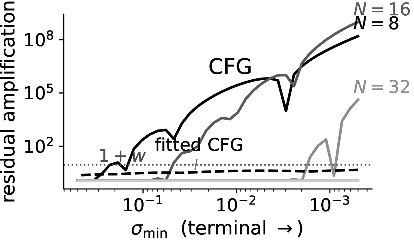
Our primary residual and image-quality comparisons fix their schemes, cells, and metrics before each run; the feature-space, latent-diffusion, and dense-reference results are exploratory diagnostics. The single-coordinate Gaussian diagnostic isolates the theorem’s singular mechanism: on uniform log-\(\sigma\) meshes with \(a=0<b\), CFG develops the coarse-mesh branch of Theorem 1 while the fitted coefficient stays below Proposition 4’s finite-tax bound (Figure 2). In the default \(w\)–\(N\) sweep, worst-case amplification reaches \(10^3\)–\(10^9\) for CFG but stays \(\le4.66\) for the fitted step, below each \(1+w\) bound—a theorem figure, not a learned-checkpoint quality metric.
4.0.0.2 Real-checkpoint residual diagnostics.
We then test the coefficient as a drop-in replacement on NVIDIA edm CIFAR-10 VP checkpoints [8] (the ‘VP’ label is network preconditioning only; sampling uses the \(\sigma\)-parameterization): \(D_{\mathrm{c}}\) is the class-conditional checkpoint, \(D_{\mathrm{u}}\) the separately trained unconditional one, and both schemes use the same Karras mesh, seeds, labels, and NFE. The grid is \(w\in\{4,6.5,8\}\) and \(N\in\{8,16,32\}\), with two 64-seed blocks (class \(0\), seeds from \(1000\); class \(1\), from \(2000\)). Table ¿tbl:tab:real-checkpoint-gate? reports paired fitted/CFG ratios for the amplification median and tail, and paired clipping differences; lower is better.
In both blocks, for every tested \(N\in\{8,16,32\}\) at \(w=6.5\) and \(w=8\), fitted CFG improves the amp median, amp p95, and clipping median. The hardest cell is the clearest: at \(w=8,N=8\), the class-\(0\) amp median/p95 falls from \(4.57/13.35\) under CFG to \(1.41/1.71\) under fitted CFG, while the clipping median drops from \(0.379\) to \(0\); the class-\(1\) replicate matches (amp p95 ratio \(0.116\), clipping delta \(-0.23\)). At \(w=4\), where the theory predicts a much weaker tax, the median amplification is mixed, but the amp tail and saturation proxy still improve in most cells. We use this as evidence for high-guidance stabilization, not uniform superiority at weak guidance.
4.0.0.3 Image-quality evaluation.
We next ran two 5000-image balanced-class evaluations on the hard cell \(w=8,N=8\), plus a 50k replication, each including a terminal-interval baseline (vanilla CFG correction off when \(h>h_\flat\), after [7]; on this coarse mesh every step crosses \(h_\flat\), so it reduces to unguided conditional DDIM). We score with FID and KID (feature-space quality metrics; lower is better). Table 1 collects the results. Fitted CFG has the best FID in all three blocks at zero extra NFE, and the certificates replicate (amp p95 falls from \(13{+}\) to \({\approx}1.6\), clipping p95 from \({\approx}0.57\) to \(0\)). The metrics disagree, however: KID is lowest for CFG in every block. We therefore read this as support for high-guidance stabilization and FID improvement, not an unqualified image-quality win; feature-manifold and sharpness diagnostics are consistent with CFG’s oversaturation contributing to the split (Figure 3), and a DINOv2 backbone-swapped audit gives the same fitted-favoring ordering, so the split is not Inception-specific (Appendices 9 and 10).
| scheme | FID \(\downarrow\) | KID \(\downarrow\) | amp p95 \(\downarrow\) | clip p95 \(\downarrow\) | target acc \(\uparrow\) | |
|---|---|---|---|---|---|---|
| 5k (A) | CFG | \(32.44\) | \(\mathbf{0.0110}\) | \(13.32\) | \(0.570\) | \(94.96\) |
| fitted | \(\mathbf{25.22}\) | \(0.0181\) | \(1.66\) | \(0\) | \(94.66\) | |
| interval | \(26.46\) | \(0.0224\) | \(1.63\) | \(0\) | \(89.24\) | |
| 5k (B) | CFG | \(31.98\) | \(\mathbf{0.0107}\) | \(13.20\) | \(0.572\) | \(94.88\) |
| fitted | \(\mathbf{24.89}\) | \(0.0173\) | \(1.64\) | \(0\) | \(94.34\) | |
| interval | \(26.04\) | \(0.0211\) | \(1.62\) | \(0\) | \(90.00\) | |
| 50k | CFG | \(27.86\) | \(\mathbf{0.0108}\) | \(13.34\) | \(0.569\) | \(95.14\) |
| fitted | \(\mathbf{20.88}\) | \(0.0177\) | \(1.65\) | \(0\) | \(94.83\) | |
| interval | \(22.08\) | \(0.0221\) | \(1.63\) | \(0\) | \(88.95\) |

Finally, the target-accuracy column of Table 1 is a classifier-conditionality diagnostic (classifier at \(94.37\%\) on the CIFAR-10 test set): in every block fitted CFG stays within \(0.6\)pp of CFG yet \({\sim}5\)pp above interval, keeping CFG’s conditional pull without its clipping pathology.
4.0.0.4 Robustness grid.
The 50k replication (Table 1) reduces the 5k-sampling-artifact concern for the FID ordering, and the KID split persists at scale. A nine-cell grid (\(w\in\{4,6.5,8\}\), \(N\in\{8,16,32\}\), 5k images each) shows it is not cell-specific: fitted CFG improves FID in \(9/9\) cells, clipping p95 in \(9/9\), and amp p95 in \(8/9\) (exception \(w{=}4,N{=}32\), both near \(1\)). The terminal-interval baseline wins FID at \(N\in\{16,32\}\) and KID at \(N=32\) but loses conditionality everywhere (\(3.24\)–\(5.72\)pp).
4.0.0.5 Interval-baseline separation.
Is the fitted step just guidance shutdown? We compared it against a tuned conditionality-preserving limited interval (selected per cell) and the parameter-free terminal interval (Appendix 11). In the tested cells, the tuned interval preserves target accuracy but does not beat the fitted step on FID; the terminal interval can win FID (e.g.\(12.63\) vs \(17.12\) at \(w{=}8,N{=}16\)) but drops target accuracy by \(5\)–\(6\)pp. So the fitted step gives interval-like residual stabilization while keeping the guided update active—it is not explained away by turning guidance off.
4.0.0.6 All-class audit.
Extending the residual diagnostic from two classes to all ten CIFAR-10 classes on the high-guidance cells (60 class–cell pairs), clipping/saturation is non-increased in \(60/60\) pairs and amp p95 improves in \(54/60\): global saturation robustness and near-global residual-tail improvement (Appendix 13).
4.0.0.7 Latent-diffusion smoke.
The mechanism is not specific to pixel-space CIFAR. On Stable Diffusion 1.5 DDIM at high guidance, the same coefficient sharply reduces pixel saturation (p95 \(0.134\to0.009\) at guidance \(12\), over 256 images) while preserving CLIP image–text alignment (\(0.320\to0.314\)); terminal guidance shutdown reaches lower saturation but collapses CLIP to \(0.271\) (Appendix 12). This is a cross-domain smoke test, not a Stable Diffusion benchmark.
5 Related work↩︎
The CFG-repair family is crowded, and methods differ mainly in their mathematical object: a manifold projection, a guidance-vector rescaling, an interval schedule, a dynamic weight, or—ours—a terminal fitted-operator coefficient. In brief: CFG++ [10] constrains the update to the data manifold; limited-interval guidance [7] switches guidance off outside a \(\sigma\) band (Remark 3 derives its terminal edge parameter-free); APG [6] down-weights the update’s parallel component; CFG-Zero\(^\star\) [11] optimizes the scale and zero-inits early steps; and C\(^2\)FG [12] decays the weight in time. None derives the terminal-fitted coefficient \(r^{1+w}-r\) from the guided exponent—where the barrier lives. An orthogonal line analyses what the continuous guided law samples—CFG is a predictor–corrector, not a sampler of its tilted target [4], [5]—the “model” bill complementary to ours.
6 Discussion and limitations↩︎
6.0.0.1 What is proved.
On the commuting class-subset Gaussian model, the barrier (Theorem 1) is sharp; the fitted step is consistent, sign-preserving, terminal-exact, pays only a finite \(O(1+w)\) crossover tax (Prop. 4), and is first-order accurate on the crossover (Theorem 2)—all about the discretization against the guided flow’s own pushforward, AP in \(\sigma_{\min}\) but not uniform in \(w\).
6.0.0.2 What is evidence.
On learned CIFAR-10 edm checkpoints, fitted CFG is a drop-in, zero-extra-NFE high-guidance stabilizer: the certificates improve residual amplification and clipping across every \(w\in\{6.5,8\}\) cell; the hard-cell evaluations (5k twice, 50k once) give it the best FID with target accuracy preserved, and a DINOv2 backbone-swap the same ordering; the nine-cell grid gives \(9/9\) FID wins over CFG. It separates from tuned and terminal interval baselines (which either lose target accuracy or fail to beat it on FID), holds across all ten classes (\(60/60\) saturation non-increase, \(54/60\) amp-tail), and transfers to Stable Diffusion 1.5 DDIM as a saturation-reducing coefficient that keeps CLIP alignment far better than guidance shutdown (Section 4, Appendices 11–13).
6.0.0.3 What is neither.
We do not claim (i) an unqualified image-quality win—KID stays lowest for CFG at 5k and 50k, a split tied to CFG’s oversaturation without proven causation; (ii) that CIFAR verifies the sharp threshold law—the learned diagnostics are only consistent with the model ordering; or (iii) a 50k KID win or many-cell large-sample result—the 50k run is one hard cell. Nor is the fitted step a uniformly better integrator of the vanilla CFG field on learned checkpoints: against a \(512\)-step CFG reference its residual tails shrink but its final-image \(L_2\) does not (Appendix 14), an interval can win FID in some cells by weakening guidance, and the Stable Diffusion result is a smoke test, not a benchmark. The class-subset hypothesis is itself a boundary: where the class is wider than the marginal, the continuous guided flow is unstable (exponent \(-w\)), which no solver can repair (Remark [rem:reverse]).
6.0.0.4 Scope and outlook.
Every certificate uses only sampler-computed quantities from two separate checkpoints, so shared-head correlations cannot inflate them. ‘Asymptotic-preserving’ is used in the calibration-model sense: on learned checkpoints we audit AP-relevant residuals rather than certify AP. Next: shared-dropout CFG, broader latent-diffusion benchmarks, and a whole-model accuracy theory.
Reproducibility Statement↩︎
All theoretical results are stated with explicit constants on the model of Hypothesis 1, and complete proofs appear in Appendix 7.
Every empirical diagnostic in Section 4 is produced by a self-contained script operating on the public NVIDIA edm CIFAR-10 VP checkpoints with stated seeds, meshes, sample counts,
schemes, and metrics; the synthetic-crossover and checkpoint-certificate scripts additionally ship CPU --self-test modes, and the synthetic crossover figure requires no checkpoints. The supplementary package contains the scripts, the exact
commands, the run manifests, and all summary artifacts (CSV/JSON) behind every number reported in the paper, including the 50k and nine-cell grid diagnostics.
7 Deferred proofs↩︎
Proof of Proposition 1. For \(a=0\) one has \(A \equiv 1\), so \(\mu_w = (1+w) - wB = 1 + w(1-B) = 1 + wb/(b+\sigma^2)\); the limits and monotonicity are immediate. Cases (i) and (ii) follow from \(A, B \to 1\) and \(A, B \to 0\) respectively. ◻
Proof of Lemma 1. Integrate (4 ): \(\int \mu_w \,\mathrm{d}\log\sigma = \tfrac{1+w}{2} \log(a+\sigma^2) - \tfrac{w}{2}\log(b+\sigma^2)\) up to a constant, since \(\mathrm{d}\log(c+\sigma^2) = 2A_c\,\mathrm{d}\log\sigma\) with \(A_c = \sigma^2/(c+\sigma^2)\). Exponentiate the increment. ◻
Proof of Theorem 1. From (10 ): \(G_w > 0 \iff \mathrm{e}^{-h} > w/(1+w) \iff h < \log(1+1/w)\), which is (a). For (b), on the pure layer \(\eta_{w}\propto \xi/\sigma\), so the residual ratio per step is \(|\xi_{n+1}/\xi_n| \cdot \sigma_n/\sigma_{n+1} = |G_w|\mathrm{e}^{h}\). On the branch \(G_w \le 0\) this is \((w - (1+w)\mathrm{e}^{-h})\mathrm{e}^{h} = w\mathrm{e}^{h} - (1+w)\), which exceeds \(1\) iff \(\mathrm{e}^{h} > 1 + 2/w\); on the branch \(G_w \ge 0\) it equals \((1+w) - w\mathrm{e}^{h} \le 1\) always. Compounding over \(\Lambda_\varepsilon/h\) steps gives (12 ). For (c), \(G_w \le 1\) always, and \(G_w \ge -1 \iff (1+w)\mathrm{e}^{-h} \ge w-1\), vacuous for \(w \le 1\) and equivalent to \(h \le h_\infty\) otherwise. The ordering \(h_\sharp < h_\infty\) follows from \(\frac{1+w}{w-1} - \bigl(1+\frac{2}{w}\bigr) = \frac{2}{w(w-1)} > 0\). ◻
Proof of Proposition 2. \(r^{1+w} - r = \mathrm{e}^{-(1+w)h} - \mathrm{e}^{-h}\) and \(w(r-1) = w(\mathrm{e}^{-h}-1)\); both are \(-wh + O(h^2)\), and expanding to second order, \(r^{1+w}-r-w(r-1) = \mathrm{e}^{-(1+w)h}-(1+w)\mathrm{e}^{-h}+w = \tfrac 12 w(w+1)h^2 + O(h^3)\). ◻
Proof of Proposition 3. On an eigen-coordinate, \(D_{\mathrm{c}}= (1-A)\xi\), \(x-D_{\mathrm{c}}= A\xi\), and \(D_{\mathrm{u}}- D_{\mathrm{c}}= (A-B)\xi\); substituting into (15 ) gives the first expression in (?? ), and regrouping \(1 - A + rA - r(A-B) + r^{1+w}(A-B)\) gives the second. Nonnegativity of each term is \(0 \le B \le A \le 1\) and \(0 < r < 1\). The regime values and the \(r \to 0\) limit are read off termwise. ◻
Proof of Lemma 2. On shared normals \((A,B)=(1,1)\) one has \(D_{\mathrm{u}}-D_{\mathrm{c}}=0\), so every scalar coefficient gives the DDIM factor \(r\). On tangent directions \((A,B)=(0,0)\), both denoisers equal the state and every coefficient gives factor \(1\). On a pure discriminative normal \((A,B)=(1,0)\), the factor of the scalar update is \(r+\alpha(r,w)\). Exactness requires \(r+\alpha(r,w)=r^{1+w}\), hence the displayed coefficient, uniquely. ◻
Proof of Proposition 4. For \(a=0\), \(A\equiv 1\) and \(q=1-B\). The decomposition (?? ) gives the coordinate factor \[G_{\rm fit} = r_nB_n+r_n^{1+w}(1-B_n) = r_n\bigl[(1-q_n)+r_n^{\,w}q_n\bigr].\] Since \(\eta_{w}=\mu(\sigma)\xi/\sigma\), the residual ratio is \((\mu_{n+1}/\mu_n)(G_{\rm fit}/r_n)\), which is (?? ). The bracket is at most \(1\) because \(0\le q_n\le 1\) and \(0<r_n^w\le 1\), so products telescope: \[\prod_{n=0}^{k-1} \frac{|\eta_{w}(\xi_{n+1},\sigma_{n+1})|}{|\eta_{w}(\xi_n,\sigma_n)|} \le \prod_{n=0}^{k-1}\frac{\mu_{n+1}}{\mu_n} = \frac{\mu_k}{\mu_0} \le 1+w .\] ◻
Theorem 2 (first-order guided AP on the discriminative crossover). On a discriminative Gaussian coordinate (\(a=0<b\)), for \(w\ge0\) and a uniform \(\lambda\)-mesh of step \(0<h\le1\), the fitted step (15 ) and the exact guided flow satisfy \(\xi_K^{\rm fit}=\Theta_K\,\xi_K^{\rm ex}\) with \(0\le\log\Theta_K\le\tfrac{1+h}{4}\,w(w+2)\,h\), hence \(W_2\bigl(\mathrm{Law}(\xi_K^{\rm fit}),\mathrm{Law}(\xi_K^{\rm ex})\bigr) \le\bigl(\mathrm{e}^{w(w+2)h/2}-1\bigr)(\mathbb{E}|\xi_0|^2)^{1/2}\). The multiplier bound and its prefactor are independent of \(b\), \(K\), and \(\sigma_{\min}\) (the \(W_2\) scale carries the initial second moment \((\mathbb{E}|\xi_0|^2)^{1/2}\)): on this crossover the fitted step is first-order uniformly accurate against the exact flow’s own pushforward, though the \(O(w^2)\) prefactor is not uniform in \(w\).
Proof. On \(a=0\) the exact one-step factor (Lemma 1) is \(\Phi_n=r^{1+w}\bigl((1+u_n)/(1+r^2u_n)\bigr)^{w/2}\), with \(u_n=\sigma_n^2/b\), \(r=\mathrm{e}^{-h}\); the fitted factor (Proposition 3, \(A=1\)) is \(G_n=\mathrm{e}^{-h}(u_n+\mathrm{e}^{-wh})/(1+u_n)\). Writing \(y_n=\log u_n\), \(\delta(h,y):=\log(G_n/\Phi_n) = wh+\log(\mathrm{e}^{y}+\mathrm{e}^{-wh})-\bigl(1+\tfrac w2\bigr)\log(1+\mathrm{e}^{y}) +\tfrac w2\log(1+\mathrm{e}^{y-2h})\). Then \(\delta(0,y)=\partial_h\delta(0,y)=0\) (first-order consistency, Proposition 2), and with \(F(y)=\mathrm{e}^{y}/(1+\mathrm{e}^{y})^2\) one has \(\partial_h^2\delta=w^2F(y+wh)+2wF(y-2h)\ge 0\); hence \(\delta\ge 0\), so \(\Theta_K=\prod_n\mathrm{e}^{\delta(h,y_n)}\ge 1\), and Taylor’s formula gives \(\delta(h,y_n)=\int_0^h(h-s)\bigl[w^2F(y_n+ws)+2wF(y_n-2s)\bigr]\,ds\). On the uniform mesh \(y_{n+1}=y_n-2h\); since \(\int F=1\) and \(\mathrm{TV}(F)=\tfrac 12\), the rectangle bound gives \(2h\sum_n F(y_n+c)\le 1+h\) for every shift \(c\), so \(\log\Theta_K\le\int_0^h(h-s)\tfrac{1+h}{2h}(w^2+2w)\,ds=\tfrac{1+h}{4}w(w+2)h\). Synchronous coupling with \(|\xi_K^{\rm ex}|\le|\xi_0|\) (the exact discriminative factor contracts) gives the \(W_2\) bound. ◻
8 The reverse ordering↩︎
This appendix expands Remark [rem:reverse].
If a reversed singular direction has \(b = 0 < a\)—the marginal collapsed where the class has not—then the exponent (4 ) tends to \(-w\), negative for every \(w > 0\): the guided flow itself expands the coordinate as \(\sigma \to 0\), so no discretization can be uniformly stable because the continuous target is not. More generally, reverse ordering with \(0 < b < a\) can create finite-\(\sigma\) expansion windows, but only the reversed singular case creates this terminal instability. This is a property of the guidance target, not of the solver; the class-subset hypothesis excludes it by assumption, and autoguidance-style constructions aim to enforce the same directionality.
9 Metric-split diagnostics↩︎
To interpret the FID/KID split at the hard cell, we computed post-hoc feature-manifold and sharpness diagnostics on the same images. Fitted CFG improves Inception precision/recall over CFG in both 5k blocks (e.g. \(0.799/0.474\) versus \(0.704/0.360\)); interval has higher recall but lower precision. The pixel-saturation median is \(0.16\) for CFG and \(0\) for fitted CFG and interval, and the median Laplacian energy drops by an order of magnitude—consistent with the fitted step removing oversaturated high-frequency artifacts (we use the Laplacian only as an oversaturation proxy, not as evidence of sharpness). The DINOv2 audit below is a backbone-swapped control on the same split.
10 DINOv2 feature audit↩︎
To test whether the FID/KID split is Inception-specific, we recompute feature-space distances with a DINOv2 backbone (dinov2_vits14, CLS-token features; images bilinearly resized to \(224\)) against \(50\)k CIFAR-10 training images. We report the Fréchet distance FD-DINOv2 and an unbiased RBF-kernel MMD (median-heuristic bandwidth, \(100\) subsets of size \(1000\)). On the two 5k hard-cell blocks, FD-DINOv2 for CFG/fitted/interval is \(469.73/230.00/257.88\) and \(469.10/227.86/254.25\), and the DINO-MMD is \(0.0258/0.0126/0.0168\) and \(0.0257/0.0125/0.0164\); both favor fitted CFG in both blocks. FD-DINOv2 is the clean backbone-only control; the MMD changes both backbone and kernel relative to
Inception KID, so it is corroborating, not a direct KID analogue.
11 Tuned limited-interval baselines↩︎
The Section 4 interval baseline is the parameter-free terminal cutoff, which on the hard mesh reduces to unguided conditional DDIM. To test whether a tuned interval that preserves conditionality can match the fitted step, we selected per cell the conditionality-viable guidance interval \([\sigma_{\rm lo},\sigma_{\rm hi}]\) from a nine-candidate grid (the one whose target accuracy stays closest to CFG), then scored it on a fresh 5k block. Table 2 reports CFG, the fitted step, the tuned interval, and the terminal interval. In the tested cells, a conditionality-preserving tuned interval does not beat the fitted step on FID; the terminal interval can win FID in a cell (\(w{=}8,N{=}16\): \(12.63\) vs \(17.12\)) but pays a clear target-accuracy cost. The fitted step gives interval-like residual stabilization while keeping the guided update active. (Target accuracy is a classifier proxy; the high fitted value at \(N{=}16\) should not be read as fuller conditional fidelity, as it may partly reflect reduced diversity.)
| cell | scheme | FID \(\downarrow\) | KID \(\downarrow\) | amp p95 \(\downarrow\) | clip p95 \(\downarrow\) | target acc \(\uparrow\) |
|---|---|---|---|---|---|---|
| \(w{=}8,N{=}8\) | CFG | \(32.21\) | \(0.0105\) | \(13.31\) | \(0.575\) | \(95.5\) |
| fitted | \(25.70\) | \(0.0180\) | \(1.66\) | \(0\) | \(94.9\) | |
| tuned int. | \(34.25\) | \(0.0205\) | \(1.71\) | \(0.018\) | \(95.3\) | |
| terminal int. | \(26.68\) | \(0.0225\) | \(1.63\) | \(0\) | \(89.1\) | |
| \(w{=}8,N{=}16\) | CFG | \(30.83\) | \(0.0117\) | \(7.30\) | \(0.664\) | \(93.8\) |
| fitted | \(17.12\) | \(0.0070\) | \(1.66\) | \(0.006\) | \(99.3\) | |
| tuned int. | \(30.18\) | \(0.0120\) | \(1.75\) | \(0.257\) | \(98.8\) | |
| terminal int. | \(12.63\) | \(0.0072\) | \(1.66\) | \(0.000\) | \(94.8\) | |
| \(w{=}6.5,N{=}8\) | CFG | \(25.36\) | \(0.0057\) | \(8.08\) | \(0.394\) | \(98.4\) |
| fitted | \(25.36\) | \(0.0175\) | \(1.40\) | \(0\) | \(94.8\) | |
| tuned int. | \(32.60\) | \(0.0208\) | \(1.43\) | \(0.002\) | \(94.7\) | |
| terminal int. | \(26.57\) | \(0.0216\) | \(1.38\) | \(0\) | \(89.8\) |
12 Latent-diffusion transfer smoke (Stable Diffusion 1.5)↩︎
As a cross-domain check that the coefficient is not specific to pixel-space CIFAR edm, we ran a small Stable Diffusion 1.5 DDIM smoke test at high guidance, swapping only the terminal guidance coefficient. We report pixel saturation (95th percentile of the clipped-pixel fraction) and CLIP image–text alignment; the interval baseline is terminal guidance shutdown. Table 3 shows the fitted step sharply reduces saturation while preserving CLIP alignment far better than shutdown—the same saturation-repair pattern as on CIFAR. This is a smoke/deepen test, not a Stable Diffusion benchmark.
Setup. We use runwayml/stable-diffusion-v1-5 at \(512\times512\) with deterministic DDIM (\(\eta=0\), \(\epsilon\)-prediction) and
float16, over a fixed list of everyday-scene captions (repeated to \(256\) and \(128\) prompts) with no negative prompt and seeds matched across schemes. The fitted step swaps only the
terminal guidance coefficient; the interval baseline disables the guidance correction on the terminal steps below the same \(h_\flat\)-derived cutoff. Saturation p95 is the 95th percentile over images of the fraction of
final RGB pixels at the valid-range extremes; CLIP alignment uses openai/clip-vit-base-patch32.
| setting | scheme | saturation p95 \(\downarrow\) | CLIP mean \(\uparrow\) |
|---|---|---|---|
| \(g{=}12\), \(N{=}12\) (256 img) | CFG | \(0.134\) | \(0.320\) |
| fitted | \(0.009\) | \(0.314\) | |
| interval | \(0.001\) | \(0.271\) | |
| \(g{=}7.5\), \(N{=}20\) (128 img) | CFG | \(0.098\) | \(0.321\) |
| fitted | \(0.028\) | \(0.319\) | |
| interval | \(0.005\) | \(0.278\) |
13 All-class residual audit↩︎
The real-checkpoint residual diagnostic (Table ¿tbl:tab:real-checkpoint-gate?) uses class 0 and class 1 blocks. To rule out class cherry-picking, we extended it to all ten CIFAR-10 classes on the high-guidance cells (\(w\in\{6.5,8\}\), \(N\in\{8,16,32\}\); 60 class–cell pairs, all fixed before the run). Clipping/saturation is non-increased in \(60/60\) pairs, and amp p95 improves in \(54/60\); the other six are modestly worse on the amp tail (ratios \(1.02\)–\(1.25\), largest class 4 at \(w{=}6.5,N{=}8\)), with clipping still non-increased there. We describe this as global saturation robustness and near-global residual-tail improvement, and leave the raw counts for the reader to weigh.
14 Dense guided-flow reference↩︎
Theorem 2 is an accuracy statement against the exact guided flow’s own pushforward on the calibration model. On learned checkpoints this does not extend to final-image accuracy: measured against a \(512\)-step vanilla-CFG reference trajectory, the fitted step is not uniformly closer in final denoised-image \(L_2\) (Table 4, ratios \(>1\)), even though its residual and amp tails are far smaller (ratios \(\ll1\)). So the learned-checkpoint evidence supports terminal residual/saturation repair, not a claim that the fitted step is a uniformly better coarse integrator of the vanilla CFG field.
| cell | image rel-\(L_2\) med | image rel-\(L_2\) p95 | residual rel-\(L_2\) p95 | amp p95 |
|---|---|---|---|---|
| \(w{=}8,N{=}8\) | \(1.143\) | \(1.109\) | \(0.329\) | \(0.124\) |
| \(w{=}8,N{=}16\) | \(1.332\) | \(1.170\) | \(0.884\) | \(0.233\) |