Pure Nash Equilibria in Graphical Games of Bounded Width Revisited
July 08, 2026
Abstract
We revisit the complexity of deciding whether a graphical game admits a pure Nash equilibrium (PNE) parameterized by standard measures of the input graph, such as treewidth. The natural dynamic programming algorithm for this problem has parameter dependence \(\alpha^{(\Delta+1)\mathrm{tw}}\) where \(\alpha\) is the maximum number of strategies available to each player, each player’s utility depends on at most \(\Delta\) other players, and the input graph has width \(\mathrm{tw}\). Our first contribution is to point out that an algorithm by Thomas and van Leeuwen [Algorithmica 2015] claiming to improve this dependence to \(\alpha^{O(\mathrm{tw})}\) is flawed and, more strongly, such an algorithm would imply that =[1].
We then set out to pinpoint the fine-grained complexity of this problem with respect to standard parameters and show that the natural DP algorithm is not optimal, as the problem can be solved with dependence \(\alpha^{ \mathchoice {\textstyle \lfloor\frac{2\Delta}{3}+1\rfloor} {\lfloor\frac{2\Delta}{3}+1\rfloor} {\lfloor\frac{2\Delta}{3}+1\rfloor} {\lfloor\frac{2\Delta}{3}+1\rfloor} {}\mathrm{tw}}\), \(\alpha^{ \mathchoice {\textstyle\lfloor\frac{\Delta}{2}+1\rfloor} {\lfloor\frac{\Delta}{2}+1\rfloor} {\lfloor\frac{\Delta}{2}+1\rfloor} {\lfloor\frac{\Delta}{2}+1\rfloor} {}\mathrm{pw}}\), and \(\alpha^{\mathrm{ctw}}\), where \(\mathrm{pw},\mathrm{ctw}\) are the pathwidth and cutwidth of the input respectively. Our main algorithmic tool is a tightening of the relationship between the width of a graph \(G\), its maximum degree, and the width of \(G^2\), which may be of independent interest. Complementing these results, we show that our algorithms for pathwidth and cutwidth are likely to be optimal, as improving them is equivalent to falsifying the \(\mathrm{pw}\)-SETH.
1 Introduction↩︎
The computation of Nash equilibria is a central topic at the intersection of computer science and economics. In this paper we focus on equilibria in graphical games, that is, games involving \(n\) players represented by the vertices of a (di-)graph whose edges indicate player interactions, in the sense that the presence of an arc \((u,v)\) indicates that the utility of player \(u\) (partially) depends on the strategy of player \(v\) (and the absence of an arc indicates that \(u\) is indifferent to \(v\)’s actions). This is an extremely natural and well-studied model [1]–[3].
The question we are interested in is the complexity of deciding whether a given graphical game admits a pure Nash equilibrium (PNE), that is, a joint strategy where no player can unilaterally increase her utility by changing her strategy. This problem is -complete [4], so we attack it using the tools of parameterized complexity, which is one of the most established approaches for dealing with NP-hardness1. Our goal is to investigate the structural parameterized complexity of deciding if a graphical game admits a PNE, for standard parameters such as treewidth, pathwidth, cutwidth and maximum degree.
This question is of course anything but new and in fact its study goes back more than twenty years. In particular, the works of Gottlob, Greco, and Scarcello [6] and Daskalakis and Papadimitriou [7] established the following: if we are given a graphical game \(\mathcal{G}\) where each player has at most \(\alpha\) available strategies, each player’s utility depends on at most \(\Delta\) other players, and we are supplied a tree decomposition of the game graph with width \(\mathrm{tw}\), then a PNE (if one exists) can be found in time \(\alpha^{(\Delta+1)\mathrm{tw}}|\mathcal{G}|^{O(1)}\). Even though the two works arrive at this complexity through different paths (CSPs of bounded hypertreewidth for [6] and Markov Random Fields for [7]), the heart of the two algorithms is essentially the natural dynamic programming approach: for each bag we need to remember the strategies of the players in the bag (\(\alpha^{\mathrm{tw}}\)) and their (out-)neighbors (\(\alpha^{\Delta\mathrm{tw}}\)). Is this algorithm optimal?
This important question was taken up by Thomas and van Leeuwen [8]. Their main (purported) contribution was an algorithm significantly improving upon the performance of the two previous algorithms by removing the dependence on \(\Delta\). Specifically, they claim that the problem can be decided in time \(\alpha^{O(\mathrm{tw})}|\mathcal{G}|^{O(1)}\). As some dependence on \(\Delta\) remains in the \(|\mathcal{G}|^{O(1)}\) factor2, their algorithm attempts to separate the exponential dependence on \(\mathrm{tw}\) from the exponential dependence on \(\Delta\). To the best of our knowledge, this has so far been accepted as the current state of the art (for instance [9]). A main motivation of our paper is the observation that this result is, in fact, flawed, and indeed no such algorithm is possible under standard hypotheses.
Our results
Our goal in this paper is two-fold: to clarify the state of the art with respect to the structural parameterized complexity of the fundamental problem of computing PNEs in graphical games; and to give a fine-grained investigation of the precise complexity of this problem with respect to some of the most important parameters.
With respect to the first goal, our main result is that the algorithm of [8] contains a serious flaw. More strongly, we show that even when \(\alpha=2\), the problem is [1]-hard parameterized by treewidth (or even by vertex cover), which implies that if the algorithm of [8] were correct, then =[1]. Therefore, a parameter dependence of the form \(\alpha^{(\Delta+1)\mathrm{tw}}\), as given by [6], [7], is more likely to be close to the correct answer.
Motivated by this, we then set out to identify the correct parameter dependence as precisely as possible. On the algorithmic side, the \(\alpha^{(\Delta+1)\mathrm{tw}}\) dependence of the algorithms of [6], [7] is natural, as it keeps the information necessary to ensure that when a vertex is forgotten the corresponding player is locally stable (does not wish to deviate). Despite this, we show that the natural approach is in fact not optimal and its parameter dependence can be improved by a constant factor in the exponent. Our algorithmic results are as follows:
Theorem 1. The existence of a PNE in a graphical game \(\mathcal{G}\), where players have at most \(\alpha\) strategies and utilities depending on at most \(\Delta\) other players, can be decided in time:
\(\alpha^{ \mathchoice {\textstyle \lfloor\frac{2\Delta}{3}+1\rfloor} {\lfloor\frac{2\Delta}{3}+1\rfloor} {\lfloor\frac{2\Delta}{3}+1\rfloor} {\lfloor\frac{2\Delta}{3}+1\rfloor} \mathrm{tw}}\cdot|\mathcal{G}|^{O(1)}\) where \(\mathrm{tw}\) is the width of a given tree decomposition;
\(\alpha^{ \mathchoice {\textstyle\lfloor\frac{\Delta}{2}+1\rfloor} {\lfloor\frac{\Delta}{2}+1\rfloor} {\lfloor\frac{\Delta}{2}+1\rfloor} {\lfloor\frac{\Delta}{2}+1\rfloor} {}\mathrm{pw}}\cdot|\mathcal{G}|^{O(1)}\) where \(\mathrm{pw}\) is the width of a given path decomposition;
\(\alpha^{\mathrm{ctw}}\cdot|\mathcal{G}|^{O(1)}\) where \(\mathrm{ctw}\) is the width of a given cutwidth ordering.
The main takeaway is that we decrease the exponent of the parameter dependence by a factor of roughly \(2\) and \(\frac{3}{2}\) respectively for pathwidth and treewidth, which is done by tightening the constants in a well-known relationship between the widths of a graph and its square. Given that our algorithmic improvement is based on an immediate application of a combinatorial relation, it is then important that we can establish our results to be (likely) essentially optimal for pathwidth and cutwidth. In particular, we show the following:
Theorem 2. The following statements are equivalent:
The \(\mathrm{pw}\)-SETH is false.
There exists an odd integer \(\Delta\ge 3\), an integer \(\alpha\ge 2\) and \(\varepsilon>0\) such that the existence of a PNE in a graphical game \(\mathcal{G}\), where each player has at most \(\alpha\) strategies and her utility depends on at most \(\Delta\) other players can be decided in time \((\alpha-\varepsilon)^{ \mathchoice {\textstyle\lfloor\frac{\Delta}{2}+1\rfloor} {\lfloor\frac{\Delta}{2}+1\rfloor} {\lfloor\frac{\Delta}{2}+1\rfloor} {\lfloor\frac{\Delta}{2}+1\rfloor} {}\mathrm{pw}}\cdot|\mathcal{G}|^{O(1)}\) where \(\mathrm{pw}\) is the width of a given path decomposition.
There exists an integer \(\alpha\ge 2\) and \(\varepsilon>0\) such that the same problem can be decided in time \((\alpha-\varepsilon)^{\mathrm{ctw}}\cdot|\mathcal{G}|^{O(1)}\) where \(\mathrm{ctw}\) is the width of a given cutwidth ordering.
The \(\mathrm{pw}\)-SETH states that the standard dynamic programming algorithm for SAT parameterized by pathwidth, which has parameter dependence \(2^{\mathrm{pw}}\), cannot be improved to \((2-\varepsilon)^{\mathrm{pw}}\). Observe that Theorem 2 not only establishes that improving the algorithms of Theorem 1 for pathwidth and cutwidth is impossible under the \(\mathrm{pw}\)-SETH, but in fact shows that such an improvement is equivalent to falsifying the \(\mathrm{pw}\)-SETH. The lower bound for pathwidth of course also automatically applies to treewidth, which leaves it as an intriguing open question whether we can obtain a better lower bound for treewidth or a better algorithm.
Techniques
With respect to techniques, the main contribution of this paper is a tightening of a well-known combinatorial relation between the width of a graph \(G\), its maximum degree, and the width of \(G^2\). Before we describe this, let us explain the context through which this question enters the picture. We are given as input a digraph \(G\) with \(n\) vertices, representing the players. A natural way to decide if a PNE exists is to construct a CSP instance with \(n\) variables of domain \(\alpha\) (one variable for each player) and add for each player \(u\) a constraint that includes \(u\) and all her out-neighbors and is satisfied only in joint strategies where \(u\) does not wish to deviate. The primal graph of this instance can be obtained from \(G\) by turning the out-neighborhood of every vertex into an undirected clique; we denote this graph as \(G^{\mathrm{\sffamily co}}\) and call it the co-neighbor graph of \(G\). Observe that if \(G\) is undirected (or bi-directed), \(G^{\mathrm{\sffamily co}} = G^2\), where vertices at distance at most \(2\) in \(G\) are adjacent.
The natural next step is to solve the CSP instance. To this end, if we bound the treewidth of \(G^{\mathrm{\sffamily co}}\), we can use a standard algorithm with dependence \(\alpha^{\mathrm{tw}({G^{\mathrm{\sffamily co}}})}\). The treewidth of \(G^{\mathrm{\sffamily co}}\) (and the treewidth of \(G^2\)) can easily be upper-bounded by \((\Delta+1)(\mathrm{tw}(G)+1)\) by taking a tree decomposition of \(G\) and adding to each bag that contains a vertex \(u\) all (out-)neighbors of \(u\). This is well-known, explicitly stated in [7] Lemma 4.5, [10], [11] Theorem 12, [12] Lemma 1, [13] Lemma 6.0.2, [14] Lemma 4.1, and used implicitly throughout the literature, e.g., [15]. Furthermore, this upper bound seems in a sense tight, as \(\mathrm{tw}(K_{1,n}^2)=\mathrm{tw}(K_{n+1})=n\cdot \mathrm{tw}(K_{1,n})\).
Our main algorithmic contribution is to show that the above standard bound is not tight, and can in fact be improved by a constant factor. To the best of our knowledge, this was not known before, which we find quite surprising since the combinatorial relation between \(\mathrm{tw}(G),\Delta(G)\), and \(\mathrm{tw}(G^2)\) is well-known and has often been used algorithmically as mentioned. More precisely we prove the following:
Theorem 3. For any digraph \(G\) of maximum out-degree \(\Delta\) we have:
\(\mathrm{tw}(G^{\mathrm{\sffamily co}})\le \mathchoice {\textstyle \lfloor\frac{2\Delta}{3}+1\rfloor} {\lfloor\frac{2\Delta}{3}+1\rfloor} {\lfloor\frac{2\Delta}{3}+1\rfloor} {\lfloor\frac{2\Delta}{3}+1\rfloor} {}\mathrm{tw}(G)+2\lfloor\frac{2\Delta}{3}\rfloor\);
\(\mathrm{pw}(G^{\mathrm{\sffamily co}})\le \mathchoice {\textstyle\lfloor\frac{\Delta}{2}+1\rfloor} {\lfloor\frac{\Delta}{2}+1\rfloor} {\lfloor\frac{\Delta}{2}+1\rfloor} {\lfloor\frac{\Delta}{2}+1\rfloor} {}\mathrm{pw}(G)+2\lfloor\frac{\Delta}{2}\rfloor\);
\(\mathrm{pw}(G^{\mathrm{\sffamily co}})\le \mathrm{ctw}(G)+\Delta\).
Furthermore, the above bounds are constructible.
Even though in this paper we focus on digraphs, we observe that we obtain a corollary for undirected graphs which is likely to be of independent interest. This follows immediately from Theorem 3 by considering an undirected graph as a bi-directed digraph.
Corollary 1. For any undirected graph \(G\) of maximum degree \(\Delta\) we have:
\(\mathrm{tw}(G^{2})\le \mathchoice {\textstyle \lfloor\frac{2\Delta}{3}+1\rfloor} {\lfloor\frac{2\Delta}{3}+1\rfloor} {\lfloor\frac{2\Delta}{3}+1\rfloor} {\lfloor\frac{2\Delta}{3}+1\rfloor} {} \mathrm{tw}(G)+2\lfloor\frac{2\Delta}{3}\rfloor\);
\(\mathrm{pw}(G^{2})\le \mathchoice {\textstyle\lfloor\frac{\Delta}{2}+1\rfloor} {\lfloor\frac{\Delta}{2}+1\rfloor} {\lfloor\frac{\Delta}{2}+1\rfloor} {\lfloor\frac{\Delta}{2}+1\rfloor} {} \mathrm{pw}(G)+2\lfloor\frac{\Delta}{2}\rfloor\).
Interestingly, we are able to establish for both pathwidth and treewidth that the results of Corollary 1 (and therefore also of Theorem 3) are essentially tight by giving an infinite family of examples. Therefore, it is not possible to squeeze any further improvement by bounding the width of \(G^{\mathrm{\sffamily co}}\) (or \(G^2\)) and our algorithms are optimal under this approach.
To establish the optimality of our algorithms in the general sense, we give reductions from CSPs of appropriate alphabets for the pathwidth and cutwidth cases, showing that improving our algorithms would falsify the \(\mathrm{pw}\)-SETH. Notably, one advantage of our algorithmic approach of reducing to a CSP is that this also automatically implies a reduction in the other direction, showing that improving our algorithms is equivalent to falsifying the \(\mathrm{pw}\)-SETH.
Finally, let us mention that we focus on digraphs, because this allows a more fine-grained exploration of the problem’s complexity, but in general we refer to undirected graph width parameters. These correspond to the width of the underlying graph, that is, the graph obtained by ignoring directions. Focusing on digraphs makes our algorithmic results stronger, as the previous works giving the less efficient \(\alpha^{(\Delta+1)\mathrm{tw}}\) parameter dependence [6], [7] were focusing on the special case when the input is undirected (bi-directed). Conversely, it is worth noting that our reduction showing that the problem is [1]-hard parameterized by treewidth produces bi-directed graphs, which is exactly the case purportedly solved by [8] in time.
Other related work
The problem of computing PNEs is a well-studied topic and computing equilibria is generally hard, even in the parameterized setting and especially if one is also looking to optimize some objective [4], [16]–[22]. Mixed equilibria, which are guaranteed to exist, are also -hard to compute even for graphical games of pathwidth \(2\) [23]. In this paper we focus on undirected structural parameters, even though the input is a digraph, as directed analogues of treewidth are known to be unhelpful for this problem [1].
The \(\mathrm{pw}\)-SETH was recently put forward by Lampis [24] as a more solid alternative to the SETH and shown to be equivalent to numerous tight lower bounds for problems parameterized by pathwidth. It is implied by weaker versions of the SETH and the Set Cover Conjecture [25], and has recently been used as a starting point for tight lower bounds [26]–[30]. We also remark that the vast majority of problems have the same complexity parameterized by pathwidth and treewidth [31]–[33], making the gap we have between \(\frac{1}{2}\) and \(\frac{2}{3}\) more intriguing.
Paper organization
After some preliminaries in Section 2, we explain in Section 3 why the results of [8] are flawed. Then, in Section 4.1 we present our combinatorial bounds, their algorithmic applications, as well as examples showing the tightness. In Section 5 we present our lower bounds based on the \(\mathrm{pw}\)-SETH and close with some discussion in Section 6.
2 Preliminaries↩︎
A graphical game is a tuple \(\mathcal{G}=(G,\{M_v\}_{v\in V(G)})\). \(G\) is the digraph with each vertex corresponding to one player and each arc indicating a utility dependency. Let \(N^{+}(v)\) be the set of out-neighbors of \(v\), \(N^{+}[v]=N^{+}(v)\cup\{v\}\) be the closed out-neighborhood of \(v\). Then the utility of player \(v\) is determined by the strategies of \(N^{+}[v]\), and is given by the payoff matrix \(M_v\). Let \(\mathrm{St}(v)\) be the set of available strategies for player \(v\), then \(M_v\) is a matrix mapping \(\mathrm{St}(v)\times \prod_{u\in N^{+}(v)}\mathrm{St}(u)\) to \(\mathbb{R}\). Given a joint strategy \(\mathbf{s}\) of \(V(G)\), for each player \(v\), we say \(v\) is locally stable if changing her strategy will not increase the utility, i.e., \[\forall x\in \mathrm{St}(v), \quad M_v(\mathbf{s}|_{v},\mathbf{s}|_{N^{+}(v)})\ge M_v(x,\mathbf{s}|_{N^{+}(v)}),\label{eq:vertex-stable}\tag{1}\] where \(\mathbf{s}|_v, \mathbf{s}|_U\) denote the (joint) strategy of a player \(v\), a set of players \(U\) in \(\mathbf{s}\) respectively. Our problem is to decide whether a given graphical game admits a pure Nash equilibrium (PNE), that is, a joint strategy of all players in which everyone is locally stable. For simplicity, we say a graphical game is an \(\alpha\)-strategy game if every player has at most \(\alpha\) strategies. Moreover, any structural properties (e.g., width, maximum degree) of a game implicitly refer to its underlying game graph. Now we give the remaining two key concepts in our work.
Definition 1 (co-neighbor graph). Given a digraph \(G\), we define the co-neighbor graph of \(G\), denoted by \(G^{\mathrm{\sffamily co}}\), as the undirected graph with the same vertex set as \(G\) and an edge between two vertices \(u\) and \(v\) if and only if there is a vertex \(w\) such that \(\{u,v\} \subseteq N^{+}[w]\).
Note that co-neighbor graph is a generalization of the square graph to digraphs, and the moral graph [34] to cyclic digraphs.
Definition 2 (Constraint satisfaction problem). A constraint satisfaction problem is defined as a triple \(\langle X, \Sigma, C \rangle\), where \(X\) is a finite set of variables, \(\Sigma\) is a finite alphabet, and \(C\) is a finite set of constraints of the form \(\langle t_j, R_j \rangle\), where \(t_j\) is a tuple of distinct variables from \(X\) and \(R_j \subseteq \Sigma^{|t_j|}\). The problem asks whether there exists an assignment \(\sigma: X \to \Sigma\) such that for every constraint \(\langle t_j, R_j \rangle \in C\) with \(t_j = (x_1, \dots, x_{|t_j|})\) we have \((\sigma(x_1), \dots, \sigma(x_{|t_j|})) \in R_j\).
Finally, recall that when we talk about the width of a digraph, we are referring to the width of the underlying undirected graph. This graph is not necessarily simple, as if both arcs \((u,v)\) and \((v,u)\) exist, they form parallel edges in the underlying undirected graph. Multiple edges do not affect the pathwidth and treewidth, but they do affect the cutwidth as it counts the number of edges instead of vertices.
3 W[1]-hardness parameterized by vertex cover↩︎
In this section, we explain why the algorithmic result of [8] is flawed. They claim:
The existence of a PNE in an undirected \(\alpha\)-strategy graphical game \(\mathcal{G}\) with treewidth \(\mathrm{tw}\) can be decided in time \(\alpha^{\mathrm{tw}}|\mathcal{G}|^{O(1)}\).
In contrast, we prove the problem is [1]-hard parameterized by vertex cover, which is an upper bound of treewidth, and therefore the [1]-hardness also applies to treewidth.
Theorem 4. Determining the existence of a PNE in an undirected 2-strategy graphical game is [1]-hard parameterized by vertex cover.
Proof. We reduce from Multicolored Clique. Given a \(k\)-partite graph \(G\) with vertex partition \(V_1\cup V_2\cup \dots \cup V_k\) and each \(V_i\) is of size \(n\), we build an undirected graphical game \((G',\{M_v\}_{v\in V(G')})\) where \(G'\) has a vertex cover of size at most \(3k^2\) such that there exists a PNE in the game if and only if there exists a clique of size \(k\) in \(G\).
For each part \(V_i\), we create an independent set of size \(\ell=\lceil\log_2 n\rceil\), \(v_{i,1},v_{i,2},\dots,v_{i,\ell}\). The joint strategy of these \(\ell\) players encodes a choice of vertex in \(V_i\). Then for every pair of \(V_{i_1},V_{i_2} (i_1<i_2)\), we create three players \(u_{i_1i_2,1},u_{i_1i_2,2},u_{i_1i_2,3}\), and add edges from \(u_{i_1i_2,1}\) to \(v_{i,j}\) for all \(i\in \{i_1,i_2\}, j\in[\ell]\), and set up \(u_{i_1i_2,2},u_{i_1i_2,3}\) as a conditional matching pennies gadget forcing \(u_{i_1i_2,1}\) to play \(1\)3. \(M_{u_{i_1i_2,1}}\) is defined such that it plays \(1\) if and only if the joint strategy of \(v_{i_1,1},\dots,v_{i_1,\ell},v_{i_2,1},\dots,v_{i_2,\ell}\) encodes a pair of vertices that are adjacent in \(G\), and \(M_{v_{i,j}}\) is a constant matrix. Note that each player in this graph interacts with at most \(\max\{2\ell+2,k-1\}\) other players, so the construction of the payoff matrices can be done in time \(2^kn^{O(1)}\), resulting in an reduction. Finally, it is easy to see \(\{u_{i_1i_2,h}\}_{1\le i_1<i_2\le k,h\in [3]}\) is a vertex cover of size at most \(3k^2\). So if there is an algorithm for PNE parameterized by vertex cover, then we can decide the existence of a clique of size \(k\) in time. ◻
Besides [clm:tw-alg], we observe that [8] contains a second flawed algorithmic claim. In particular, they claim to give a polynomial-time algorithm when the maximum number of strategies \(\alpha=2\) (even for games of unbounded degree and treewidth). However, this is not possible (unless ¶=) due to [4].
Theorem 5 ([4]). Determining the existence of a PNE in an undirected graphical game is -complete, even if it is \(2\)-strategy with maximum degree \(3\).
Besides the hardness result, we give some further notes in Appendix ¿sec:app:notes-on-thomas?.
Further Notes on [8]↩︎
To complete the discussion of Section 3 let us also roughly explain where the error lies in the analysis of their treewidth algorithm. They claim that the main idea of their dynamic program is to record for each vertex in the bag not only its strategy in the current partial solution, but also its optimal response to the strategies of its forgotten neighbors. Intuitively, this seems unlikely to work as in order to calculate the best response, one would also need to take into account the strategies of neighbors that have not yet been introduced. Furthermore, in their analysis they claim that when a vertex is forgotten we update the payoff matrices of its neighbors to only keep information consistent with the strategy of the forgotten vertex. This would, however, need to keep a different version of the payoff matrix for each combination of strategies of the forgotten neighbors of a vertex, which is not taken into account in the running time analysis.
To be more concrete, consider the following game graph and an associated tree decomposition:
Figure 1: 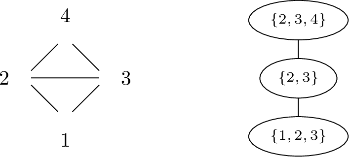 .
.
Each player has two strategies. The payoff matrices of the players are defined so that \(2\) wants to play the same strategy as \(3\) if \(1\) and \(4\) play the same strategy and wants to play the opposite strategy of \(3\) otherwise, while \(3\) wants to play the same strategy as \(2\) if \(1\) and \(4\) play different strategies and wants to play the opposite strategy of \(2\) otherwise. \(1\) and \(4\) have constant payoff matrices. Then when \(1\) is forgotten, no constraint is added to the choice of \(2\) and \(3\). Therefore, when \(4\) is introduced, \(2,3\) and \(4\) have no constraint on their strategies, and the algorithm would conclude that there is a PNE, which is apparently not the case.
4 On the width of (generalized) graph squares↩︎
In this section, we prove our upper bounds on the different width parameters of \(G^{\mathrm{\sffamily co}}\), yielding three algorithms for computing PNEs parameterized by \(\mathrm{pw},\mathrm{tw},\mathrm{ctw}\) respectively. After that, we give examples showing our bounds are essentially tight for \(\mathrm{pw}\) and \(\mathrm{tw}\).
4.1 Upper bounds↩︎
We present three combinatorial upper bounds on the width of \(G^{\mathrm{\sffamily co}}\) as a function of the maximum out-degree and the width of \(G\). Let us first give some intuition starting from pathwidth. Recall that it is easy to establish that \(\mathrm{pw}(G^{\mathrm{\sffamily co}})\le (\Delta+1)(\mathrm{pw}(G)+1)\) simply by adding all the out-neighbors of any vertex to each bag that contains it. Our approach starts with an attempt of not adding all the out-neighbors. For each vertex \(u\), and for each bag \(X\) that contains \(u\), either the minority (at most \(\lfloor \frac{\Delta}{2}\rfloor\)) of its out-neighbors have been introduced in bags before \(X\); or the minority of its out-neighbors are introduced in later bags. In either case, we add to \(X\) whichever subset of out-neighbors forms the minority. This gives us a decomposition of width at most \((1+\lfloor\frac{\Delta}{2}\rfloor)(\mathrm{pw}(G)+1)\), with a significant problem that no bag contains all the closed out-neighborhood of \(u\), which induce a clique in \(G^{\mathrm{\sffamily co}}\). To fix this, we observe that \(u\) transitions from having the minority to the majority of its neighbors already introduced in a pair of consecutive bags. We can therefore insert a bag between the two, adding all the out-neighbors of \(u\) and paying a second \(\lfloor \frac{\Delta}{2}\rfloor\) additive term.
The trick above also generalizes to treewidth, but the perfect balance of the out-neighborhood between the “left” and “right” parts is no longer possible. In contrast, the best to achieve with this trick is to “save” one third of the out-neighborhood of each vertex. Intuitively, this is inevitable because there may be a join bag (a bag of degree \(3\)) in which each vertex has one third of its out-neighbors in each of the three directions in the decomposition.
Finally, the bound for cutwidth is more straightforward where the path decomposition is constructed by adding to each bag the heads of arcs crossing a cut in a cutwidth ordering.
Theorem 6. For a digraph \(G\) with maximum out-degree \(\Delta\) we have \[\mathrm{pw}(G^{\mathrm{\sffamily co}})\le \mathchoice {\textstyle\lfloor\frac{\Delta}{2}+1\rfloor} {\lfloor\frac{\Delta}{2}+1\rfloor} {\lfloor\frac{\Delta}{2}+1\rfloor} {\lfloor\frac{\Delta}{2}+1\rfloor} {}\mathrm{pw}(G)+2\lfloor\textstyle\frac{\Delta}{2}\rfloor.\label{eq:pw-sqr-ub}\qquad{(1)}\] Furthermore, given a path decomposition of \(G\) of width \(\mathrm{pw}\), a path decomposition of \(G^{\mathrm{\sffamily co}}\) of width at most \(\mathchoice {\textstyle\lfloor\frac{\Delta}{2}+1\rfloor} {\lfloor\frac{\Delta}{2}+1\rfloor} {\lfloor\frac{\Delta}{2}+1\rfloor} {\lfloor\frac{\Delta}{2}+1\rfloor} {}\mathrm{pw}+2\lfloor\textstyle\frac{\Delta}{2}\rfloor\) can be found in polynomial time.
Proof. Assume we are given a nice path decomposition \(\mathcal{P}=(X_1, X_2, \ldots, X_r)\) of \(G\) of width \(\mathrm{pw}\). We will construct a path decomposition \(\mathcal{P}^{\mathrm{\sffamily co}}\) for \(G^{\mathrm{\sffamily co}}\) with the claimed width. Let \(\lambda=\lceil{\frac{\Delta}{2}}\rceil\) be a threshold parameter. We scan the bags from left to right, then in each bag \(X_i\) and for a vertex \(v\in X_i\), \(N^{+}(v)\) can be bipartitioned as follows:
\(N^{\preceq}_i(v)\): the present neighbors of \(v\) that are either in the current bag or have been forgotten;
\(N^{\succ}_i(v)\): the future neighbors of \(v\) that are still to be introduced in the future.
For a vertex \(v\), suppose it is introduced and forgotten in bags \(i_v\) and \(f_v+1\), respectively. Then, \[N^{\preceq}_{i_v}(v) =X_{i_v}\cap N^{+}(v), \qquad N^{\preceq}_{f_v}(v) =N^{+}(v), \qquad N^{\preceq}_{i}(v) \subseteq N^{\preceq}_{i+1}(v), \forall i_v\le i < f_v.\]
Figure 2: 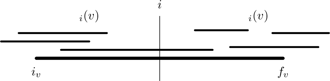 .
.
The statements above follow from the fact that every neighbor of \(v\) must appear together with \(v\) in a bag, and from the connectivity constraint on bags that contain each specific vertex in a path decomposition. We say a vertex \(v\) is heavy in bag \(X_i\) if \(v\in X_i\) and \(|N^{\preceq}_i(v)|\ge \lambda\). Let \(L_i\subseteq X_i\) be the set of vertices that are light in \(X_i\). Note that the transition from light to heavy is a one-way process because \(|N^{\preceq}_i(v)|\) is non-decreasing as \(i\) increases.
Now we scan the bags of \(\mathcal{P}\) from left to right, and iteratively append new bags to \(\mathcal{P}^{\mathrm{\sffamily co}}\). For each bag \(X_i\), we let \(B_{i,1}, B_{i,2}, \dots, B_{i,m_i}\) be the sequence of bags we append when processing \(X_i\). For \(X_i\) introducing a vertex \(v\), let \(t_1,t_2,\dots,t_{\ell}\) be the list of vertices that become heavy in \(X_i\). It is worth noting that \(v\) is also possibly heavy, if sufficiently many neighbors of \(v\) are already in \(X_{i-1}\). We now create a sequence of \(m_i=2\ell+1\) bags. For the \(2k\)-th bag \((k\in [\ell])\), we introduce all vertices in \(N^{+}[t_k]\), and in the subsequent bag, we forget every present neighbor of \(t_k\) that is already forgotten and does not belong to the present neighborhood of some other (temporarily) light vertex in \(L_i\cup\{t_{k+1},\dots,t_{\ell}\}\)4. Formally (let \(B_{i,1}=B_{i-1,m_{i-1}}\cup \{v\}\)), \[\begin{align} \forall 1\le k\le \ell: \quad B_{i,2k} = & B_{i,2k-1}\cup N^{\succ}_i(t_k) \tag{2} \\ \quad B_{i,2k+1} = & B_{i,2k}\setminus \left(N^{\preceq}_i(t_k)\setminus N^{\preceq}_i(L_i\cup \{t_{k+1},\dots,t_{\ell}\})\right),\tag{3} \end{align}\] where \(N^{\preceq}_i(S)\) is defined as \(\bigcup_{u\in S}N^{\preceq}_i(u)\). For \(X_i\) forgetting \(v\), if \(v\in N^{\preceq}_i(L_i)\), we simply neglect this bag, i.e., \(m_i=0\) and let \(B_{i,0}=B_{i-1,m_{i-1}}\); otherwise, we append a new bag that forgets \(v\), i.e., \(m_i=1\) and \(B_{i,1}=B_{i-1,m_{i-1}}\setminus \{v\}\). We claim for each \(i\in [|\mathcal{P}|]\), \(B_{i,m_i}=X_i\cup \bigcup_{v\in L_i} N^{\preceq}_i(v) \cup \bigcup_{v\in X_i\setminus L_i} N^{\succ}_i(v),\) which shows such bags have size at most \(\mathchoice {\textstyle\lfloor\frac{\Delta}{2}+1\rfloor} {\lfloor\frac{\Delta}{2}+1\rfloor} {\lfloor\frac{\Delta}{2}+1\rfloor} {\lfloor\frac{\Delta}{2}+1\rfloor} {}(\mathrm{pw}+1)\), and the same bound can also be shown for \(B_{i,2k+1}\), and thus the size of \(B_{i,2k}\) can have an additional \(O(\Delta)\) term, giving the desired bound. Full proof of validity and width analysis can be found in Appendix ¿sec:app:pw-sqr-ub?. ◻
The validity and width of the construction in 6↩︎
We first show the \(\mathcal{P}^{\mathrm{\sffamily co}}\) constructed by the procedure in the proof of 6 is a valid path decomposition for \(G^{\mathrm{\sffamily co}}\). It is easy to see every vertex is covered. For an edge \((u,v)\in E(G^{\mathrm{\sffamily co}})\), either \((u,v)\in E(G)\), or there exists \(w\) such that \(u,v\in N^{+}(w)\). In the first case, this edge is covered by 2 when \(t_k=u\). In the second case, this edge is covered by 2 when \(t_k=w\). Finally, to show every vertex appears in a contiguous segment, it suffices to prove that each vertex is only forgotten once. If \(v\) is forgotten in \(B_{i,*}\) for some \(i\) in \(\mathcal{P}^{\mathrm{\sffamily co}}\), then either \(X_i\) forgets \(v\) while \(v\not\in N^{\preceq}_i(L_i)\); or \(X_i\) is an introduce bag where \(v\) is no longer in \(N^{\preceq}_i(L_i)\) with \(v\) already forgotten. To conclude, \(v\) is forgotten in \(B_{i,*}\) if and only if \(X_i\) is a bag that \[v\not\in X_i \wedge v\not\in N^{\preceq}_i(L_i) \wedge (v\in X_{i-1} \vee v\in N^{\preceq}_{i-1}(L_{i-1})).\] Suppose there exists another bag \(X_{i'}\) satisfying the constraint above and without loss of generality we assume \(i<i'\). \(v\) is already forgotten in \(X_i\), so \(v\not\in X_{i'-1}\), therefore \(v\in N^{\preceq}_{i'-1}(L_{i'-1})\) must hold. Let \(u\in X_{i'-1}\) be a vertex such that \(v\in N^{\preceq}_{i'-1}(u)\). Suppose \(u\) is introduced before \(X_i\), then since \(v\in N^{\preceq}_{i'-1}(u)\), we also have \(v\in N^{\preceq}_i(u)\), and thus \(v\in N^{\preceq}_i(L_i)\), which contradicts the assumption. Otherwise, suppose \(u\) is introduced at or after \(X_{i}\), then since \(v\) has been forgotten, the edge \((u,v)\) is not covered by any bag. We thus proved such \(X_i\) is unique, and each vertex is only forgotten once.
Now it remains to analyze the width of \(\mathcal{P}^{\mathrm{\sffamily co}}\). It is easy to see
For each \(i\in [|\mathcal{P}|]\), we have \[B_{i,m_i}=X_i\cup \bigcup_{v\in L_i} N^{\preceq}_i(v) \cup \bigcup_{v\in X_i\setminus L_i} N^{\succ}_i(v).\]
Then it follows that \[\begin{align} |B_{i,m_i}|\le & (\mathrm{pw}+1)+(\lambda-1)|L_i|+(\Delta-\lambda)(\mathrm{pw}+1-|L_i|) \\ = & (\Delta-\lambda+1)(\mathrm{pw}+1)+(2\lambda-\Delta-1)|L_i| \\ \le & \mathchoice {\textstyle\lfloor\frac{\Delta}{2}+1\rfloor} {\lfloor\frac{\Delta}{2}+1\rfloor} {\lfloor\frac{\Delta}{2}+1\rfloor} {\lfloor\frac{\Delta}{2}+1\rfloor} {} (\mathrm{pw}+1), \end{align}\] For intermediate bags, we have
For each \(i\in [|\mathcal{P}|]\) s.t. \(m_i\ge 3\), let \(\ell=\frac{m_i-1}{2}\). Then for any \(k(0\le k \le \ell)\), \[B_{i,2k+1}=X_i\cup \bigcup_{v\in L_i\cup \{t_{k+1},\dots,t_{\ell}\}} N^{\preceq}_i(v) \cup \bigcup_{v\in X_i\setminus L_i\setminus \{t_{k+1},\dots,t_{\ell}\}} N^{\succ}_i(v).\]
Since \(N^{\preceq}_i(t_{*})\) intersects \(X_i\) in at least one vertex (\(v\)), we have \(|N^{\preceq}_i(t_{*})\setminus X_i|\le \lambda-1\), giving \[\begin{align} |B_{i,2k+1}|\le & (\mathrm{pw}+1)+(\lambda-1)(|L_i|+\ell-k)+(\mathrm{pw}+1-(|L_i|+\ell-k))(\Delta-\lambda) \\ \le & \lfloor\textstyle\frac{\Delta}{2}+1\rfloor (\mathrm{pw}+1). \end{align}\] It then follows that \[\begin{align} |B_{i,2k}|\le & |B_{i,2k-1}|+\Delta-\lambda \\ \le & \lfloor\textstyle\frac{\Delta}{2}+1\rfloor (\mathrm{pw}+1)+\lfloor\textstyle\frac{\Delta}{2}\rfloor. \end{align}\]
Theorem 7. For a digraph \(G\) with maximum out-degree \(\Delta\), we have \[\mathrm{tw}(G^{\mathrm{\sffamily co}})\le \mathchoice {\textstyle \lfloor\frac{2\Delta}{3}+1\rfloor} {\lfloor\frac{2\Delta}{3}+1\rfloor} {\lfloor\frac{2\Delta}{3}+1\rfloor} {\lfloor\frac{2\Delta}{3}+1\rfloor} {}\mathrm{tw}(G)+2\lfloor \textstyle \frac{2\Delta}{3}\rfloor.\] Furthermore, given a tree decomposition of \(G\) of width \(\mathrm{tw}\), a tree decomposition of \(G^{\mathrm{\sffamily co}}\) of width at most \(\mathchoice {\textstyle \lfloor\frac{2\Delta}{3}+1\rfloor} {\lfloor\frac{2\Delta}{3}+1\rfloor} {\lfloor\frac{2\Delta}{3}+1\rfloor} {\lfloor\frac{2\Delta}{3}+1\rfloor} {}\mathrm{tw}+2\lfloor \textstyle \frac{2\Delta}{3}\rfloor\) can be found in polynomial time.
Proof. Let \(\lambda=\lceil\frac{\Delta}{3}\rceil\). Given a nice tree decomposition \(\mathcal{T}=(T,\{X_i\}_{i\in V(T)})\), we traverse the bags in a bottom-up manner. For each bag \(X_i\) and for each vertex \(v\) in this bag, we define \(N^{\preceq}_i(v)\), \(N^{\succ}_i(v)\) and the notion of heavy as in 6. For each vertex \(v\), if it is introduced in a bag \(X_{i_v}\) and forgotten in the parent of bag \(X_{f_v}\), we have \[N^{\preceq}_{i_v}(v)= X_{i_v}\cap N^{+}(v), \qquad N^{\preceq}_{f_v}(v)= N^{+}(v), \qquad N^{\preceq}_{i}(v)\subseteq N^{\preceq}_{p(i)}(v), \forall i_v\preceq i \prec f_v,\] where \(p(i)\) is the parent of \(i\), and \(i\preceq j\) (\(i\prec j\)) denotes that \(j\) is an ancestor (a proper ancestor) of \(i\). The bags where \(v\) is heavy form a subtree rooted at \(f_v\) (denoted by \(T[v|\mathsf{heavy}]\)), and is a part of the subtree of all bags containing \(v\) (denoted by \(T[v]\)). We arbitrarily fix a unique leaf in \(T[v|\mathsf{heavy}]\), and call it the switching leaf of \(v\). Moreover, we call the path from the switching leaf to \(f_v\) the switching path of \(v\). Then for each vertex \(v\) in a bag \(X_i\), we introduce another notion of switched: \(v\) is switched in \(X_i\) when \(X_i\) belongs to the switching path of \(v\). And we let \(L_i\subseteq X_i\) to denote the set of vertices that are unswitched in \(X_i\).
Figure 3:  .
.
Now we are ready to construct a tree decomposition \(\mathcal{T}^{\mathrm{\sffamily co}}\) for \(G^{\mathrm{\sffamily co}}\). For each bag \(X_i\in \mathcal{T}\), we will construct a sequence of bags that forms a path in \(\mathcal{T}^{\mathrm{\sffamily co}}\), and denote them by \(B_{i,1},B_{i,2},\dots,B_{i,m_i}\) in a bottom-up order, and connect \(B_{i,m_i}\) to \(B_{p(i),1}\) if \(i\) is not the root.
For introduce and forget nodes, we use almost identical constructions as 6. The only difference here is for introduce nodes we apply the construction with the list of vertices having \(X_i\) as their switching leaf instead of the list of vertices that become heavy. For join node \(i\) with children \(i_1,i_2\), we first create \(B_{i,1}\) as \(B_{i_1,m_{i_1}}\cup B_{i_2,m_{i_2}}\). Note that for a vertex \(v\), its future neighbors in \(X_{i_1}\) is composed of its future neighbors in \(X_i\) and present neighbors in \(X_{i_2}\), and the latter part should be removed from the current union. \(B_{i,2}\) is thus created by iterating through all \(v\in X_i\setminus L_{i_b} (b\in \{1,2\})\) and forgetting every element in \(N^{\preceq}_{i_{3-b}}(v)\) that does not belong to the present neighborhood of some other (temporarily) unswitched vertex. Then, for the vertices \(t_1,\dots,t_{\ell}\) with \(X_i\) as the switching leaf, we create bags as introduce node case. Namely, we have \[\begin{align} B_{i,1}= & B_{i_1,m_{i_1}}\cup B_{i_2,m_{i_2}}, \\ B_{i,2}= & B_{i,1}\setminus \bigcup_{b\in \{1,2\},v\in X_i\setminus L_{i_b}} \left(N^{\preceq}_{i_{3-b}}(v)\setminus N^{\preceq}_i(L_i\cup \{t_1,\dots,t_{\ell}\})\right), \\ \forall 1\le k\le \ell: \quad B_{i,2k+1} = & B_{i,2k}\cup N^{\succ}_i(t_k), \\ \quad B_{i,2k+2} = & B_{i,2k+1}\setminus \left(N^{\preceq}_i(t_k)\setminus N^{\preceq}_i(L_i\cup \{t_{k+1},\dots,t_{\ell}\})\right). \end{align}\]
Now we show \(\mathcal{T}^{\mathrm{\sffamily co}}\) is valid. The non-trivial part is to show the bags including a certain vertex induce a subtree. It suffices to show that each vertex is forgotten only once. If \(v\) is forgotten in \(B_{i,*}\) for some \(i\), then either \(X_i\) is a bag forgetting \(v\) while \(v\not\in N^{\preceq}_i(L_i)\); or \(X_i\) is an introduce or a join bag where \(v\) is no longer in \(N^{\preceq}_i(L_i)\) with \(v\) already forgotten. Namely, \(v\) is forgotten in \(B_{i,*}\) if and only if \(X_i\) is the bag that \(v\not\in X_i\wedge v\not\in N^{\preceq}_{i}(L_i)\) and \[\begin{cases} v\in N^{\preceq}_{i_1}(L_{i_1})\vee v\in N^{\preceq}_{i_2}(L_{i_2}), & \text{if i is a join node with children i_1 and i_2}, \\ v\in X_{i_1}\vee v\in N^{\preceq}_{i_1}(L_{i_1}), &\text{if i is an introduce or forget node with child i_1.} \end{cases}\] Then we prove by contradiction that such \(i\) is unique. We first claim:
For any bag \(X_i\), if \(v\in N^{\preceq}_{i}(L_i)\), then \(\exists j\preceq i\) such that \(v\in X_j\).
By [clm:pre-s-in-bag], we can see that there exists \(j\preceq i\) such that \(v\in X_j\), and that \(v\not\in X_i\) is equivalent to \(f_v\preceq i\) in the condition for vertex \(v\) being forgotten in \(B_{i,*}\). Suppose there is another introduce or forget node \(i'\) with child \(i'_1\) satisfying the same condition, and without loss of generality, we assume \(f_v\preceq i\preceq i'_1\prec i'\). It immediately follows that \(v\not\in X_{i'}\), and thus \(v\in N^{\preceq}_{i'_1}(L_{i'_1})\). Let \(u\in L_{i'_1}\) be a vertex such that \(v\in N^{\preceq}_{i'_1}(u)\), then if \(u\) is already introduced in \(X_{i}\), then \(v\in N^{\preceq}_{i}(u)\subseteq N^{\preceq}_{i}(L_i)\), contradicting the assumption. Otherwise, edge \((u,v)\) is not covered by any bag, resulting in a violation. Now we suppose there is another join node \(i'\) satisfying the condition with children \(i'_1,i'_2\), and without loss of generality assume \(f_v \preceq i\preceq i_1'\prec i'\). Same argument as the previous case rules out the possibility of \(v\in N^{\preceq}_{i'_1}(L_{i'_1})\). If \(v\in N^{\preceq}_{i'_2}(L_{i'_2})\), then by [clm:pre-s-in-bag] there exists \(j\preceq i'_2\) such that \(v\in X_j\), which contradicts the requirement of bags containing \(v\) inducing a connected subtree. Therefore, such \(i\) is unique, and thus \(v\) is only forgotten once.
It remains to analyze the width of \(\mathcal{T}^{\mathrm{\sffamily co}}\). We claim for each \(i\in V(T)\), \(B_{i,m_i}=X_i\cup \bigcup_{v\in L_i}N^{\preceq}_i(v)\cup \bigcup_{v\in X_i\setminus L_i}N^{\succ}_i(v)\), giving \(|B_{i,m_i}|\le (\Delta-\lambda+1)(\mathrm{tw}+1) \le \mathchoice {\textstyle \lfloor\frac{2\Delta}{3}+1\rfloor} {\lfloor\frac{2\Delta}{3}+1\rfloor} {\lfloor\frac{2\Delta}{3}+1\rfloor} {\lfloor\frac{2\Delta}{3}+1\rfloor} {}(\mathrm{tw}+1)\). For a join bag \(X_i\) with children \(i_1,i_2\) (for other bags, the analysis is similar and simpler): \[\begin{align} N^{\preceq}_i(v)= & N^{\preceq}_{i_1}(v)\cup N^{\preceq}_{i_2}(v),\quad \forall v\in X_i, \\ B_{i,1}= & X_i\cup \bigcup_{v\in L_{i_1}\cap L_{i_2}}N^{\preceq}_{i}(v) \cup \bigcup_{b\in \{1,2\}, v\in X_i\setminus L_{i_b}} N^{\succ}_{i_b}(v), \\ B_{i,2}= & X_i\cup \bigcup_{v\in L_{i_1}\cap L_{i_2}}N^{\preceq}_{i}(v)\cup\bigcup_{v\in X_i\setminus (L_{i_1}\cup L_{i_2})} N^{\succ}_{i}(v), \\ B_{i,2k+1}= & X_i\cup \bigcup_{v\in L_i\cup \{t_{k+1},t_{k+2},\dots,t_{\ell}\}}N^{\preceq}_{i}(v)\cup\bigcup_{v\in X_i\setminus L_i\setminus \{t_{k+1},t_{k+2},\dots,t_{\ell}\}} N^{\succ}_{i}(v). \\ \end{align}\] For any \(v\in L_i\), if it is heavy in at least one of \(X_{i_1}, X_{i_2}\), then \(|N^{\preceq}_i(v)|\le \Delta-\lambda\) because of the existence of another bag as the switching leaf; otherwise, \(|N^{\preceq}_i(v)|\le 2\lambda-2\). Thus, \[\begin{align} |B_{i,2}|\le|B_{i,1}|\le & (\mathrm{tw}+1) + \max\{\Delta-\lambda,2\lambda-2\}|L_{i_1}\cap L_{i_2}| + (\Delta-\lambda)(\mathrm{tw}+1-|L_{i_1}\cap L_{i_2}|) \\ \le & \mathchoice {\textstyle \lfloor\frac{2\Delta}{3}+1\rfloor} {\lfloor\frac{2\Delta}{3}+1\rfloor} {\lfloor\frac{2\Delta}{3}+1\rfloor} {\lfloor\frac{2\Delta}{3}+1\rfloor} {}(\mathrm{tw}+1). \end{align}\] Similar argument gives \(|B_{i,2k+2}|\le \mathchoice {\textstyle \lfloor\frac{2\Delta}{3}+1\rfloor} {\lfloor\frac{2\Delta}{3}+1\rfloor} {\lfloor\frac{2\Delta}{3}+1\rfloor} {\lfloor\frac{2\Delta}{3}+1\rfloor} {}(\mathrm{tw}+1)\) for \(k\in [\ell]\), leading to
\(\displaystyle |B_{i,2k+1}|\le |B_{i,2k}|+\Delta-\lambda\le \mathchoice {\textstyle \lfloor\frac{2\Delta}{3}+1\rfloor} {\lfloor\frac{2\Delta}{3}+1\rfloor} {\lfloor\frac{2\Delta}{3}+1\rfloor} {\lfloor\frac{2\Delta}{3}+1\rfloor} {}(\mathrm{tw}+1)+\lfloor \textstyle \frac{2\Delta}{3} \rfloor.\) ◻
Theorem 8. For a digraph \(G\) with maximum out-degree \(\Delta\), we have \(\mathrm{pw}(G^{\mathrm{\sffamily co}})\le \mathrm{ctw}(G)+\Delta.\) Furthermore, given a linear ordering of \(G\) with cutwidth \(\mathrm{ctw}\), a path decomposition of \(G^{\mathrm{\sffamily co}}\) of width at most \(\mathrm{ctw}+\Delta\) can be found in polynomial time.
Proof. Given a linear ordering \(v_1,v_2,\ldots,v_n\) of the vertices that achieves the cutwidth \(\mathrm{ctw}\), we create a path decomposition of \(2n\) bags, and for each \(i\in [n]\) (let \(B_0=\emptyset\)), \[B_{2i-1}=B_{2i-2}\cup N^{+}[v_i],\qquad B_{2i}=B_{2i-1}\setminus \{v_j\mid j\le i, \not\exists k>i \text{ s.t. } v_j\in N^{+}(v_k)\}.\] Namely, for \(B_{2i}\), we remove all the heads which are only incident to \(v_i\) as a tail. Now we show that this is a valid path decomposition of \(G^{\mathrm{\sffamily co}}\), and it is easy to see that every vertex and edge is covered by some bag. Then we can see that \(v_i\) is introduced at \(B_{2j-1}\) if \(v_j\) is the leftmost vertex belonging to \(N^{-}[v_i]\), and is forgotten at \(B_{2k}\) if \(v_k\) is the rightmost vertex belonging to \(N^{-}[v_i]\). Therefore, it instantly follows that the bags containing \(v_i\) are consecutive.
Figure 4:  .
.
Finally, it remains to show the width of the path decomposition. Consider the set of edges that cross the cut after \(v_{i}\), and let \(H_i\) be the set of heads of these edges. We claim for each \(i\in [n]\), \(B_{2i}=H_i\), from which it immediately follows that \(|B_{2i}|\le \mathrm{ctw}\) and \(|B_{2i-1}|\le \mathrm{ctw}+\Delta+1\). This claim is equivalent to saying \[H_i=H_{i-1}\cup N^{+}[v_i]\setminus \{v_j\mid j\le i, \not\exists k>i \text{ s.t. } v_j\in N^{+}(v_k)\},\] which is true since \(H_i\setminus H_{i-1}\) contains the heads \(v_j\) incident to \(v_i\) that \(j>i\) (marked red), and \(H_{i-1}\setminus H_i\) are the heads whose rightmost in-neighbor is exactly \(v_i\) (marked blue). Note that the latter set can even include \(v_i\) itself if there is no in-neighbor of \(v_i\) to the right.
Figure 5:  .
.
◻
4.2 Algorithmic implications↩︎
Theorem 9. The existence of a PNE in an \(\alpha\)-strategy graphical game \(\mathcal{G}=(G,\{M_v\}_{v\in V(G)})\) with maximum out-degree \(\Delta\) can be encoded as a CSP instance \(\psi_{\mathcal{G}}\) with primal graph \(G^{\mathrm{\sffamily co}}\) and alphabet size \(\alpha\).
Proof. For each player \(v\), we create a variable \(x_v\) in \(\psi_{\mathcal{G}}\) whose domain is the strategy set of \(v\), and add a constraint on the variables corresponding to \(N^{+}[v]\) to ensure that \(v\) is locally stable. Namely, we create a constraint whose relation is the set of all joint strategies of \(N^{+}[v]\) that make \(v\) locally stable. Now we look at the primal graph of \(\psi_{\mathcal{G}}\). The primal graph has a vertex set \(\{x_v\mid v\in V(G)\}\), and there is an edge between \(x_u\) and \(x_v\) if they appear together in the same constraint, and this can only happen if \(u\) and \(v\) are adjacent or they have a common in-neighbor. Therefore, the primal graph of \(\psi_{\mathcal{G}}\) is exactly \(G^{\mathrm{\sffamily co}}\). ◻
Recall the result for CSPs parameterized by \(\mathrm{tw}\):
Theorem 10 ([35]). There is an algorithm that given a CSP instance \(\psi\) with \(n\) variables on alphabet \(\Sigma\), decides whether \(\psi\) is satisfiable in time \(|\Sigma|^{\mathrm{tw}+1}{|\psi|}^{O(1)}\), where \(\mathrm{tw}\) is the width of a given tree decomposition of the primal graph of \(\psi\).
10 9 6 7 8 together give the claimed three algorithmic results listed in 1. Moreover, it is known that improving the algorithm in 10 when parameterized by pathwidth is equivalent to falsifying \(\mathrm{pw}\)-SETH [24]. Therefore, if \(\mathrm{pw}\)-SETH is false, then we can improve our algorithms for PNE, giving one direction of the equivalence relation in 2.
4.3 Tightness of the bounds↩︎
In this section we show that the combinatorial upper bounds we have established are tight. In particular, the constant factors \(\frac{1}{2}\) and \(\frac{2}{3}\) in 6 7 cannot be improved. For this, we construct infinite families of graphs with maximum degree and pathwidth (treewidth) arbitrarily large such that the bounds are tight up to small additive terms.
We remark that the family we construct to show our pathwidth bound is tight is also used, with minor modifications, as the basis of our \(\mathrm{pw}\)-SETH-based lower bound. This makes sense: to obtain a tight lower bound, we need a family of graphs such that \(G^{\mathrm{\sffamily co}}\) has pathwidth as high as we estimated, because otherwise applying a CSP algorithm to our instances would solve the problem too efficiently, contradicting our lower bound.
Theorem 11. For any integers \(k, p\ge 2\), there exists a graph \(G_{k,p}\) with maximum degree \(\Delta=2k-1\) and pathwidth at most \(p+1\) such that \(\mathrm{pw}(G^2_{k,p})\ge \textstyle \mathchoice {\textstyle\lfloor\frac{\Delta}{2}+1\rfloor} {\lfloor\frac{\Delta}{2}+1\rfloor} {\lfloor\frac{\Delta}{2}+1\rfloor} {\lfloor\frac{\Delta}{2}+1\rfloor} {}\mathrm{pw}(G_{k,p})- \textstyle \mathchoice {\textstyle\lfloor\frac{\Delta}{2}+1\rfloor} {\lfloor\frac{\Delta}{2}+1\rfloor} {\lfloor\frac{\Delta}{2}+1\rfloor} {\lfloor\frac{\Delta}{2}+1\rfloor} {}.\)
Proof. Given integers \(k,p\ge 2\), we construct a graph \(G_{k,p}\) with maximum degree \(\Delta=2k-1\) and pathwidth at most \(p+1\) such that \(\mathrm{pw}(G_{k,p}^{2})\ge kp\).
We create a grid-like graph of \(n=kp\) rows and each row contains \(n\) vertices, and we denote them by \(v_{ij}\) for \(i,j\in [n]\). For the \(i\)-th row, we denote the vertices \(v_{i,gk+1} (0\le g<p)\) by the pivot vertices of this row. For each \(v_{i,gk+1}\), we connect it to \(\{v_{i,gk+2},v_{i,gk+3},\dots,v_{i,(g+1)k}\}\), and also to \(\{v_{i+1,gk+2},\dots,v_{i+1,(g+1)k}\}\) if \(i\not=n\). Finally, we connect \((v_{i,gk},v_{i,gk+1})\) for each \(i\in [n], 0< g<p\) (see below for an example for \(k=3, p=3\)).
Figure 6: 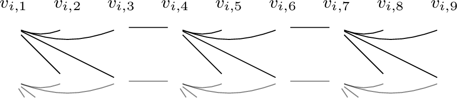 .
.
Now we give a path decomposition for \(G_{k,p}\) with width at most \(p+1\). We first iterate through the first row from left to right, and create bags to introduce the vertices one by one. If a vertex is not pivotal, we immediately forget it, with the only exception that for a vertex \(v_{1,gk}\) with \(0<g<p\), we forget it after introducing \(v_{1,gk+1}\) to cover the edge between them. After processing the first row, we stop at a bag of all the pivot vertices in the first row and all the other vertices in the first row are forgotten. Then we repeat the same process for the next rows one by one, with the only difference that we forget \(v_{i-1,(g-1)k+1}\) whenever we introduce \(v_{i,gk}\) for \(i\ge 2\) and \(0<g\le p\). Then the biggest bags are the ones containing \(v_{i,gk},v_{i,gk+1}\) for some \(i\ge 2\), which have size \(p+2\). A structured pseudocode is available in Appendix ¿sec:app:pd-1?.
Path decomposition of \(G_{k,p}\) in the proof of 11↩︎
Initialize an empty path decomposition Append a new bag introducing \(v_{1,j}\) Append a new bag forgetting \(v_{1,j-1}\) Append a new bag forgetting \(v_{1,j}\)
Append a new bag introducing \(v_{i+1,j}\)
Append a new bag forgetting \(v_{i,j-k+1}\)
Append a new bag forgetting \(v_{i+1,j-1}\) Append a new bag forgetting \(v_{i+1,j}\)
Line [line:biggest-bag] when \(j>k\) and \(j\bmod k=1\) is the step where the biggest bag in this decomposition is created, and it is of size \(p+2\), showing \(\mathrm{pw}(G_{k,p})\le p+1\).
Now we analyse the pathwidth of \(G_{k,p}^{2}\). We argue that \(G_{k,p}^{2}\) contains an \(n\times n\) grid as a subgraph, since for any \(i,j\), vertices \(v_{i,j},v_{i,j+1}\) are either connected or both adjacent to \(v_{i,k\lfloor\frac{j-1}{k}\rfloor+1}\) (the same holds for non-pivot vertices \(v_{i,j}\) and \(v_{i+1,j}\), and for pivot vertices they are both adjacent to \(v_{i+1,j+1}\)). Thus, the monotonicity of pathwidth gives
\(\displaystyle \mathrm{pw}(G_{k,p}^{2})\ge n=kp\ge \textstyle \mathchoice {\textstyle\lfloor\frac{\Delta}{2}+1\rfloor} {\lfloor\frac{\Delta}{2}+1\rfloor} {\lfloor\frac{\Delta}{2}+1\rfloor} {\lfloor\frac{\Delta}{2}+1\rfloor} {}(\mathrm{pw}(G)-1).\) ◻
Theorem 12. For any integers \(k, p\ge 2\), there exists a graph \(G_{k,p}\) with maximum degree \(\Delta=3k\) and treewidth at most \(p+1\) such that \(\mathrm{tw}(G_{k,p}^{2})\ge \textstyle \frac{2\Delta}{3}\mathrm{tw}(G_{k,p})- \textstyle \frac{2\Delta}{3}-1.\)
Similar to the previous theorem, we give a lower bound for \(\mathrm{tw}(G_{k,p}^2)\) by analyzing a specific subgraph. Since the family of these subgraphs appears to be novel to the literature, we first provide its formal definition and establish its treewidth lower bound. For any integer \(n \ge 2\), let \(T_n\) be the graph obtained by identifying one endpoint of a path \(P_n\) with each vertex of a triangle \(C_3\), and let \(H_n\) be the Cartesian product \(H_n = T_n \square P_n\) (see the diagram below for examples of \(T_3,H_3\) respectively).
Figure 7: 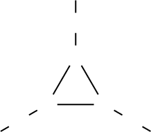 .
.
We claim the following about \(\mathrm{tw}(H_n)\), whose proof is deferred to the end of this section.
Theorem 13. For every integer \(n\ge 2\), \(\mathrm{tw}(H_n)\ge 2n-1\).
Now we start the proof of 12 assuming the validity of 13.
Proof of 12. Given integers \(k,p\ge 2\), we construct a graph \(G_{k,p}\) with maximum degree \(\Delta=3k\) and treewidth at most \(p+1\) such that \(\mathrm{tw}(G_{k,p}^{2})\ge 2kp-1\).
We use the grid-like construction in the proof of 11 as a gadget. Let \(n=kp\), we create 3 disjoint gadgets of \(n\) rows and \(n\) columns, and denote the vertices by \(\{v_{i,j}^{(h)}\mid i,j\in [n], h\in [3]\}\). Then we create an independent set of \(p\) vertices, \(r_1,r_2,\dots,r_p\), and denote them as central vertices. For each \(g\in [p]\), we add edges from \(r_g\) to \(v_{1,(g-1)k+j}^{(h)}\) for all \(j\in [k],h\in [3]\) (see below for an example with \(k=2,p=3\)).
Figure 8:  .
.
Now we give a tree decomposition of \(G_{k,p}\) with width \(p+1\) by first giving a path decomposition for the subgraph induced by \(\{r_g\}_{g\in[p]}\cup \{v_{i,j}^{(h)}\}_{i,j\in[n]}\) for each \(h\in [3]\), starting from a bag of all central vertices. We initialize the starting bag and process the first row as in the previous proof, except that \(r_g\) is forgotten when \(v_{1,gk}^{(h)}\) is introduced. Subsequent rows follow the exact same scheme, and it immediately follows that the maximum bag size remains \(p+2\) (see Appendix ¿sec:app:prof-path-decomp-tw-sqr-lb? for the full pseudocode). Finally, we can create a tree decomposition for \(G_{k,p}\) by gluing the three path decompositions together at their common starting bag.
Path decomposition for \(\{r_g\}\cup \{v_{i,j}^{(h)}\}\) in the proof of 12↩︎
Initialize a bag with all central vertices Append a new bag forgetting \(r_{g-1}\) Append a new bag introducing \(v_{1,(g-1)k+1}^{(h)}\) Append a new bag forgetting \(v_{1,(g-1)k}^{(h)}\) Append a new bag introducing \(v_{1,(g-1)k+j}^{(h)}\) Append a new bag forgetting \(v_{1,(g-1)k+j}^{(h)}\) Append a new bag forgetting \(\{r_p,v_{1,pk}^{(h)}\}\)
Append a new bag introducing \(v^{(h)}_{i+1,j}\)
Append a new bag forgetting \(v^{(h)}_{i,j-k+1}\)
Append a new bag forgetting \(v^{(h)}_{i+1,j-1}\) Append a new bag forgetting \(v^{(h)}_{i+1,j}\)
Now we analyze the treewidth of \(G_{k,p}^{2}\). We claim \(H_n\) is a subgraph of \(G_{k,p}^{2}\), because as previously argued, for any \(h\in [3]\), \(G_{k,p}^{2}\left[\{v_{*,*}^{(h)}\}\right]\) contains an \(n\times n\) grid. And for any \(j\in [n]\), \(\{v_{1,j}^{(*)}\}\subseteq N[r_{\lfloor\frac{j-1}{k}\rfloor+1}]\), so \(G_{k,p}^{2}\left[\{v_{1,j}^{(*)}\}\right]\) induce a triangle. Plugging the three grids and \(n\) triangles together gives us \(H_n\). Then the monotonicity of treewidth gives
\(\displaystyle \mathrm{tw}(G_{k,p}^{2})\ge 2n-1=2kp-1\ge \textstyle \frac{2\Delta}{3}(\mathrm{tw}(G)-1)-1.\) ◻
Now we prove 13 for completeness. We prove it by constructing a bramble of order \(2n\). We first give the formal definition of bramble, as well as its duality relation with tree decomposition, which is the main tool we use to prove 13.
Definition 3 (Bramble). A bramble* of a graph \(G\) is a family \(\mathcal{B}\) of mutually touching connected subgraphs of \(G\), i.e., for every pair \(B_1, B_2 \in \mathcal{B}\), either they share at least one vertex, or there is an edge in \(G\) with one endpoint in \(B_1\) and the other endpoint in \(B_2\). The order of a bramble \(\mathcal{B}\) is the size of its minimum hitting set.*
Theorem 14 ([36]). \(G\) has a bramble of order \(\ge k\) if and only if \(\mathrm{tw}(G)\ge k-1\).
Figure 9:  .
.
Before we start, we first define a coordinate system for the vertices of \(T_n\) and \(H_n\). We denote the vertices of \(T_n\) using a two-dimensional coordinate \((j,h), j\in [n], h\in [3]\), where \(j\) is the distance to the triangle plus \(1\) and \(h\) is the index of the path. And the vertices of \(H_n\) are denoted by \((i,j,h)\), where \(i\in [n]\) is the index of the \(T_n\) in the Cartesian product, and \(j,h\) are the coordinates in \(T_n\). We denote the first, second and third coordinate of a vertex by the level, layer and page of the vertex, respectively.
For \(i,j,h (i,j\in [n], h \in [3])\), we define \(c(i,j,h)\) to be the subgraph of \(H_n\) induced by the vertices of coordinates \((i,*,h),(i,*,h\bmod 3+1),(*,j,h)\). Intuitively, \(c(i,j,h)\) is the crossing of the following two paths:
the intersection of pages \(h,h\mod 3+1\) and level \(i\) which is a \(P_{2n}\), and
the intersection of layer \(j\) and page \(h\) which is a \(P_n\).
Now we claim the following:
The set \(\mathcal{B}=\{c(i,j,h)\mid i,j\in [n], h\in [3]\}\) is a bramble of \(H_n\).
Proof. We prove this by showing every two elements in \(\mathcal{B}\) share at least one vertex. Consider two arbitrary elements \(c(i_1,j_1,h_1), c(i_2,j_2,h_2)\) in \(\mathcal{B}\), we have the following cases:
if \(h_1=h_2\), their crossings are on the same page, so both of them pass \((i_1,j_2,h_1)\) and \((i_2,j_1,h_1)\);
if \(h_1\neq h_2\), without loss of generality we can assume \(h_2=h_1\mod 3+1\), then both of them pass \((i_1,j_2,h_2)\).
Figure 10:  .
.
Therefore, every two elements in \(\mathcal{B}\) touch each other, and \(\mathcal{B}\) is a bramble. ◻
Now we give a lower bound for the order of \(\mathcal{B}\):
Every hitting set of \(\mathcal{B}\) has size at least \(2n\).
Proof. We show any vertex set \(X\) of size \(2n-1\) fails to hit at least one element in \(\mathcal{B}\).
We first investigate the distribution of the vertices across levels. Since there are \(n\) levels and \(|X|=2n-1\), there exists a level \(i_0\) such that \(X\) contains at most one vertex in it. Without loss of generality, we assume on level \(i_0\) page \(1\) and \(2\) have no vertex in \(X\). Assuming there are a total of \(m (m\ge 0)\) vertices in \(X\) that are on page \(3\), there are no more than \(2n-m-1\) vertices in \(X\) on pages \(1\) and \(2\) in total. Now we look at pages \(1\) and \(2\). The subgraph induced by them is a grid of size \(n\times 2n\), and we know that on level (row) \(i_0\) there is no vertex in \(X\).
Figure 11:  .
.
If there exists a layer (column) \(j_0\) on page \(1\) that is not covered by any vertex in \(X\), then \(c(i_0,j_0,1)\) is not hit by \(X\). Therefore, we suppose all layers on page \(1\) are covered by \(X\). Note that this also limits \(m\le n-1\), because if \(m=n\), then the total budget for page \(1\) is \(n-1\), leaving at least one layer on page \(1\) uncovered. The budget for page \(2\) is thus \(n-m-1\), so there are at least \(m+1\) layers and levels that are not covered by \(X\). We arbitrarily pick an uncovered layer \(j_1\), then for any uncovered level \(i\), \(c(i,j_1,2)\) has to be covered by some \((i,*,3)\). However, there are \(m+1\) different such \(i\)s, and only \(m\) vertices on page \(3\), so there exists a level \(i_1\) such that \(c(i_1,j_1,2)\) is not covered by any vertex in \(X\). Therefore, \(X\) fails to hit all elements in \(\mathcal{B}\), and the hitting set of \(\mathcal{B}\) has size at least \(2n\). ◻
By [prop:bramble] and [prop:hitting-set], according to the duality between treewidth and bramble order [36], we have the lower bound for the treewidth of \(H_n\) as in 13.
5 Algorithmic lower bounds↩︎
In this section we establish that our algorithms for pathwidth and cutwidth are optimal under the \(\mathrm{pw}\)-SETH. Before we proceed let us give some intuition, focusing on the case of pathwidth. Recall that we want to justify, for each fixed values of \(\alpha,\Delta\), that parameter dependence is at least \(\left(\alpha^{\lfloor\frac{\Delta}{2}+1\rfloor}\right)^{\mathrm{pw}}\). Consider the case \(\Delta=3\), where our goal is \((\alpha^2)^\mathrm{pw}\). We will achieve this by reducing from a CSP problem with alphabet size \(\alpha\) parameterized by pathwidth. In particular, for each variable \(x\) of the initial instance and each appearance of \(x\) in a bag, we construct a player with \(\alpha\) strategies, with the goal that all these players will pick a strategy corresponding to the value of \(x\) in a satisfying assignment. It is now easy to represent each constraint; the interesting part is how to ensure that all players representing the same variable play the same strategy, while decreasing the pathwidth of the initial instance by a factor of \(2\). We can easily do this if allowed to keep the \(\mathrm{pw}\) constant, by listing the players in an \(m\times \mathrm{pw}\) grid (the left diagram), and forcing the player in row \(i\) to play the same as her copy in row \(i+1\) (and this is the essence of our cutwidth lower bound).
Figure 12:  .
.
The key idea of the pathwidth construction is now to use the larger degree to perform this information transfer more efficiently. In particular, for \(\Delta=3\), we designate every other player of a row to be a pivot player and make this player responsible for her own consistency as well as the consistency of a non-pivot player. The pivot has therefore one out-neighbor in her own row and two out-neighbors in the next row and has responsibility to ensure that this group of \(4\) players is consistent. The pivot players in each row thus become a separator (the right diagram), allowing us to decrease the pathwidth by the desired factor.
Theorem 15. For any integers \(k,\alpha\ge 2\), if there is an algorithm that given an \(\alpha\)-strategy graphical game \(\mathcal{G}\) with maximum out-degree \(\Delta=2k-1\) and pathwidth \(p\), decides whether there is a PNE in time \(\alpha^{(1-\varepsilon)k\cdot p}|\mathcal{G}|^{O(1)}\) for some \(\varepsilon>0\), then the \(\mathrm{pw}\)-SETH is false.
Proof. Suppose we are given a 3-CSP instance \(\psi\) with domain \(\Sigma\), an associated nice path decomposition for the primal graph of \(\psi\) of width \(\mathrm{pw}\) and an integer \(k\ge 2\), we build a graphical game \(\mathcal{G}=(G,\{M_v\})\) satisfying the following properties:
\(\mathcal{G}\) is \(\alpha\)-strategy where \(\alpha=|\Sigma|\) and has maximum out-degree \(\Delta=2k-1\); and
\(\mathcal{G}\) has a PNE if and only if \(\psi\) is satisfiable; and
\(\mathcal{G}\) and a path decomposition of \(G\) of width \(\frac{\mathrm{pw}}{k}+7\) can be obtained in polynomial time.
To see why this implies the theorem, suppose there exists an algorithm for PNE with runtime \(\alpha^{(1-\varepsilon)k\cdot p}|\mathcal{G}|^{C}\), then we can use this algorithm to solve the PNE instance constructed from the CSP instance in time \(\alpha^{(1-\varepsilon)k\cdot(\frac{\mathrm{pw}}{k}+7)}(n\alpha^{2k})^{C}=|\Sigma|^{(1-\varepsilon)(\mathrm{pw}+7k)+2kC}n^{C}\). When \(\mathrm{pw}>\frac{7k+2kC}{\varepsilon}\), this is \({|\Sigma|}^{(1-\varepsilon')\mathrm{pw}}n^{O(1)}\) for some \(\varepsilon'>0\), which contradicts \(\mathrm{pw}\)-SETH.
Now we give the construction. Given a path decomposition of the primal graph of \(\psi\), by adapting [24] to general CSPs and adding dummy constraints to \(\psi\), we obtain in linear time a new nice path decomposition \(B_1,\dots,B_\ell\) and a bijective function \(\mu\) from the set of constraints of \(\psi\) to the set of bags such that for each constraint \(c\), \(B_{\mu(c)}\) contains all the variables of \(c\). Under this bijection, we will check each constraint with a dedicated bag.
For all \(i\in [\ell]\) and each variable \(x_j\) in bag \(B_i\), we create a player \(v_{i,j}\) representing \(x_j\). Assuming \(B_{i}\) is used to verify a constraint containing \((x_{a_{i,1}},x_{a_{i,2}},x_{a_{i,3}})\), we then create players \(u_{i,1},u_{i,2},u_{i,3}\) and add arcs from \(u_{i,1}\) to \(v_{i,a_{i,1}},v_{i,a_{i,2}},v_{i,a_{i,3}}\), from \(u_{i,2},u_{i,3}\) to \(u_{i,1}\) and also antiparallel arcs between \(u_{i,2}\) and \(u_{i,3}\). For two consecutive bags \(B_i,B_{i+1}\), let \(B_{i}\cap B_{i+1}=\{x_1,\ldots,x_t\}\) be the set of common variables they share. Then for \(h=1,k+1,\dots,\lfloor\frac{t-1}{k}\rfloor k+1\), we create arcs from \(v_{i,h}\) to \(\left\{v_{i,h+1},v_{i,h+2},\dots,v_{i,\min(t,h+k-1)}\right\} \cup \left\{ v_{i+1,h},v_{i+1,h+1},\dots,v_{i+1,\min(t,h+k-1)}\right\}\). Two additional players \(m^{(i)}_{h,1}, m^{(i)}_{h,2}\) are introduced, with antiparallel arcs between them and arcs from \(m^{(i)}_{h,1}\) to \(v_{i,h},v_{i+1,h}\). See below for an example of \(k=3\).
Figure 13: 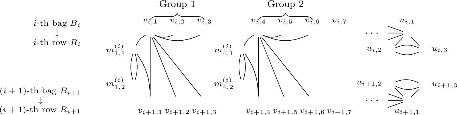 .
.
Now we construct the payoff matrices. Let \(s_{i,j}\in \Sigma\) be the strategy of \(v_{i,j}\). For \(v_{i,h}(h\in \{1,k+1,\dots\})\), the payoff matrix of \(v_{i,h}\) is defined in a way that it will want to play \(s_{i+1,h}\) if and only if \(s_{i,j}=s_{i+1,j}\) for all \(h+1\leq j \leq \min(t,h+k-1)\). For \(m^{(i)}_{h,1}\) and \(m^{(i)}_{h,2}\), we make them a conditional matching pennies gadget forcing \(v_{i,h}\) and \(v_{i+1,h}\) to play the same strategy. For \(u_{i,1}\), we make sure it plays \(1\) if and only if the joint strategy of \(v_{i,a_{i,*}}\) corresponds to a valid assignment for the constraint, and make \(u_{i,2},u_{i,3}\) a conditional matching pennies gadget forcing \(u_{i,1}\) to play \(1\). From the construction we see in any PNE, copies of each variable are consistent, and each constraint is satisfied. Finally, we give a path decomposition of width at most \(\frac{\mathrm{pw}}{k}+7\). The idea is similar to the ones used in the proof of 11, with slight changes listed as follows:
before any other players in row \(i+1\), introduce \(u_{i+1,*},v_{i+1,a_{i+1,*}}\) and forget \(u_{i+1,*}\); and
when introducing a pivot player \(v_{i+1,h}\), also introduce \(m^{(i)}_{h,*}\) and forget them right after; and
\(v_{i+1,j}\) with \(j\equiv 0\pmod k\) can be immediately forgotten.
The width can be bounded similarly. Refer to Appendix ¿sec:app:pd-pw-lb? for details. ◻
Path decomposition of the game graph in the proof of 15↩︎
Initialize a bag with \(u_{1,1},u_{1,2},u_{1,3},v_{1,a_{1,1}},v_{1,a_{1,2}},v_{1,a_{1,3}}\) Append a new bag forgetting \(u_{1,1},u_{1,2},u_{1,3}\)
Append a new bag introducing \(v_{1,j}\) Append a new bag forgetting \(v_{1,j}\)
Append a new bag introducing \(u_{i+1,1},u_{i+1,2},u_{i+1,3},v_{i+1,a_{i+1,1}},v_{i+1,a_{i+1,2}},v_{i+1,a_{i+1,3}}\) Append a new bag forgetting \(u_{i+1,1},u_{i+1,2},u_{i+1,3}\)
Append a new bag introducing \(v_{i+1,j}\) Append a new bag forgetting \(v_{i+1,j}\) Append a new bag introducing \(m^{(i)}_{j,1},m^{(i)}_{j,2}\) Append a new bag forgetting \(m^{(i)}_{j,1},m^{(i)}_{j,2}\) Append a new bag forgetting \(v_{i,j-k+1}\)
The biggest bag is created by line [line:biggest-bag-2], containing \(\lceil\frac{|B_i|}{k}\rceil\) pivot players and \(6\) others. Thus, the width of this path decomposition is at most \(\lceil \frac{|B_i|}{k}\rceil+5\le \frac{\mathrm{pw}+1}{k}+6<\frac{\mathrm{pw}}{k}+7\).
Theorem 16. For any integer \(\alpha \ge 2\), if there is an algorithm that given an \(\alpha\)-strategy graphical game \(\mathcal{G}\) with cutwidth \(\mathrm{ctw}\), decides whether there is a PNE in time \(\alpha^{(1-\varepsilon)\mathrm{ctw}}|\mathcal{G}|^{O(1)}\) for some \(\varepsilon > 0\), then the \(\mathrm{pw}\)-SETH is false.
We refer to Appendix ¿sec:app:ctw-lb? for the proof of the above theorem. These two theorems together with the result in 4.2 complete the proof of equivalence for 2.
Proof of 16↩︎
Proof. Suppose we are given a 3-CSP instance \(\psi\) with domain \(\Sigma\), an associated nice path decomposition of the primal graph of \(\psi\) with width \(\mathrm{pw}\), we build a graphical game \(\mathcal{G}=(G,\{M_v\})\) satisfying the following properties:
\(\mathcal{G}\) is \(\alpha\)-strategy where \(\alpha=|\Sigma|\); and
\(\mathcal{G}\) has a PNE if and only if \(\psi\) is satisfiable; and
\(\mathcal{G}\) and an ordering of \(V(G)\) achieving cutwidth at most \(\mathrm{pw}+4\) can be constructed in polynomial time.
If there exists an algorithm for PNE with runtime \(\alpha^{(1-\varepsilon)\mathrm{ctw}}|\mathcal{G}|^{O(1)}\), then we can use this algorithm to solve CSP in time \(|\Sigma|^{(1-\varepsilon)(\mathrm{pw}+4)}n^{O(1)}\) using the construction above, which is \(|\Sigma|^{(1-\varepsilon')\mathrm{pw}}n^{O(1)}\) for some \(\varepsilon'>0\) when \(\mathrm{pw}>\frac{4}{\varepsilon}\), contradicting \(\mathrm{pw}\)-SETH.
Now we give the construction. Similar to the proof of 15, we assume we have a bijection between the constraints and the bags in the path decomposition, and for each variable we will also make a copy for each bag it appears in, and make sure all copies of the same variable play the same strategy.
For each variable \(x_j\) in bag \(B_i\), we create a player \(v_{i,j}\) representing \(x_j\), and assume \(B_{i}\) is used to verify a constraint containing \((x_{a_{i,1}},x_{a_{i,2}},x_{a_{i,3}})\). Then create three players \(u_{i,1},u_{i,2},u_{i,3}\) and add arcs from \(u_{i,1}\) to \(v_{i,a_{i,1}},v_{i,a_{i,2}},v_{i,a_{i,3}}\), from \(u_{i,2},u_{i,3}\) to \(u_{i,1}\) and also antiparallel arcs between \(u_{i,2}\) and \(u_{i,3}\). For two consecutive bags \(B_i, B_{i+1}\) with \(B_i\cap B_{i+1}=\{x_1,\dots,x_t\}\), we create arcs \((v_{i,j},v_{i+1,j})\) for all \(j\in[t]\). The payoff matrices are defined in a way that \(v_{i,j}\) will want to play the same strategy as \(v_{i+1,j}\), \(u_{i,1}\) will only play 1 if the constraint is satisfied, and \(u_{i,2},u_{i,3}\) form a pair of matching pennies forcing \(u_{i,1}\) to play 1.
Then we have a simple layered structure where each layer corresponds to a bag in the path decomposition and checks the satisfaction status of the corresponding constraint. Therefore, we have a game graph where a PNE exists if and only if the original CSP instance is satisfiable. Moreover, the maximum out-degree in our constructed game graph is 3, so the construction can be done in polynomial time.
Finally, we give an upper bound of the cutwidth of the constructed game graph. Suppose there are \(p\) bags in total, we simply order the vertices as follows \[\begin{align} & v_{1,1},v_{1,2},\dots,v_{1,|B_1|},u_{1,1},u_{1,2},u_{1,3}, \\ & v_{2,1},v_{2,2},\dots,v_{2,|B_2|},u_{2,1},u_{2,2},u_{2,3}, \\ & \dots \\ & v_{p,1},v_{p,2},\dots,v_{p,|B_p|},u_{p,1},u_{p,2},u_{p,3}. \end{align}\]
Figure 14:  .
.
Let \(B_i\cap B_{i+1}=\{x_1,\dots,x_t\}\), then for \(v_{i,j}\), the number of arcs in the form of \((v_{i,k},v_{i+1,k})\) that cross the cut after \(v_{i,j}\) is exactly \(j\), which is at most \(\mathrm{pw}+1\). Arcs incident to \(u_{i,*}\) will make additional contribution at most 3. For \(u_{i,*}\), the number of arcs in the form of \((v_{i,j},v_{i+1,j})\) that cross the cut after \(u_{i,*}\) is exactly \(|B_i|\le \mathrm{pw}+1\), and the arcs incident to \(u_{i,*}\) will also contribute at most 3. Therefore, the cutwidth of the constructed ordering is at most \(\mathrm{pw}+4\). ◻
6 Conclusion↩︎
In this paper we established that computing a PNE is [1]-hard parameterized by standard graph parameters, such as treewidth, correcting a previous claim from the literature. We complemented this by giving optimal algorithms for this problem for parameters pathwidth and cutwidth and an improved combinatorial upper bound on the width of the square of a graph which is likely to find further applications.
The most intriguing question we leave open is the gap between the problem’s complexity for pathwidth and treewidth. As mentioned, it is extremely rare to find problems that have different complexities for these parameters. However, the gap in our tight combinatorial relations leads us to believe that PNE computation may be such a problem. Finding complexity-theoretic evidence to that effect, or conversely closing the gap by improving the treewidth-based algorithm, would therefore be very interesting. Another interesting question would be to tighten the lower bound we give for pathwidth to graphs where \(\Delta\) is even, as at the moment our bound is only tight for instances with odd degree.
References↩︎
We assume the reader is familiar with the basics of FPT algorithms as given for example in [5].↩︎
Observe that if we have \(n\) players, then the description of \(\mathcal{G}\) has size \(n\alpha^{\Delta+1}\), as for each player we are given a payoff matrix with her utility for each possible joint strategy of her closed neighborhood.↩︎
Matching pennies is a 2-player game with no PNE. Here if \(u_{i_1i_2,1}\) does not play \(1\), \(u_{i_1i_2,2},u_{i_1i_2,3}\) will simulate a matching pennies game, denying any PNE, therefore forcing \(u_{i_1i_2,1}\) to play \(1\).↩︎
We abuse the notation and also call vertices in \(t\) that have not yet been processed as temporarily light.↩︎