1 Introduction↩︎

A model trained by noisy gradient descent can be idealized as a diffusion on its loss landscape, and a basic safety question is whether the training trajectory ever enters a designated bad region of parameter space. Write \(Q_t \in \mathbb{R}^d\) for the parameters at training time \(t\) and \(\mathcal{A}_H \subseteq \mathbb{R}^d\) for a failure region: a set of parameters whose induced behavior we would like the trained model to avoid. Even when training ends safely, the trajectory can pass through \(\mathcal{A}_H\) on its way to the optimum, so the object of interest is the in-set probability \[\nu_t(\mathcal{A}_H) \;=\; \mathbb{P}(Q_t \in \mathcal{A}_H)\] at every training time \(t\), not only at convergence.

Several safety concerns share this shape. In code generation, \(\mathcal{A}_H\) is the set of parameters that emit a hidden backdoor or a known-insecure pattern, and one wants the chance that training ever lands there to be negligible. In alignment, \(\mathcal{A}_H\) is a region of misaligned or deceptive behavior that a model might drift through before settling into a benign optimum. The motivating instance for this work is the Scientist AI (SAI) Predictor safety case of [1], which separates an honest non-agentic Predictor from a scaffold that gates its outputs through a guardrail, and bounds the probability that a consequence-invariant training process produces a dangerous Predictor (one whose guarded deployment causes a designated harm event above a normative threshold) uniformly in \(t\) by \[\nu_t(\mathcal{A}_H) \;\le\; C_{\mathrm{bad}}\, R_{\mathrm{shell}}.\] Here \(R_{\mathrm{shell}}\) is the conditional fraction of dangerous Predictors inside a narrow loss band under the initialization, argued exponentially small on the grounds that danger requires many coordinated errors, and \(C_{\mathrm{bad}}\) is the within-band enrichment factor of training, assumed bounded as a stated requirement on the process. That argument treats the dynamics generating \(\nu_t\) abstractly, as a distribution over training trajectories indexed by \(t\); the present paper supplies those dynamics and bounds \(\nu_t(\mathcal{A}_H)\) directly.

We model a training run as the overdamped Langevin dynamics \[dQ_t = -\nabla J(Q_t)\, dt + \sigma\, dW_t,\] where \(J\) is the training loss on \(\mathbb{R}^d\), \(W_t\) is standard Brownian motion, and \(\sigma > 0\) is a noise level set by the optimization (informed, for example, by batch size and learning rate).

This paper proves an upper bound on the probability that the law of a Langevin training trajectory occupies the designated failure region \(\mathcal{A}_H \subseteq \mathbb{R}^d\). Under explicit smoothness, convexity, and energy-gap hypotheses on the loss \(J\), the bound is exponentially small in \(d\) and is uniform in time, after a burn-in of order \(d\). Two grades are proved: a shape-free version that uses only the total equilibrium mass \(\pi(\mathcal{A}_H)\) and the global Poincaré constant, and a shape-aware version that uses a local relaxation rate \(\lambda_{\mathcal{A}_H}\) together with a maximum-principle ceiling to remove the burn-in altogether for flux-isolated sets.

The Langevin idealization.↩︎

This SDE is the standard continuous-time model of stochastic gradient training: at small step size, minibatch SGD on a smooth loss has Itô-SDE limits with drift \(-\nabla J\) and noise covariance set by the minibatch gradient covariance [2]–[4], and the explicitly noised SGLD algorithm of [5] realizes the model used here exactly. Isotropy of the noise and the continuous-time limit are idealizations; we take them as given and do not address the discretization or anisotropy gaps.

The loss \(J\) has a minimizer \(P_n\), normalized to \(J(P_n) = 0\). We single out a failure region \(\mathcal{A}_H \subseteq \mathbb{R}^d\): a set of parameters we would like the trained model to avoid. The minimizer is safe, \(P_n \notin \mathcal{A}_H\), but the noise keeps \(Q_t\) from ever settling exactly at \(P_n\), so we must ask how much probability mass the trajectory places in \(\mathcal{A}_H\).

The natural hope is that if the failure region has small equilibrium mass \(\pi(\mathcal{A}_H)\), then \(\mathbb{P}(Q_t \in \mathcal{A}_H)\) is small for all \(t\). This hope is false in general, and the way it fails is the organizing problem of this paper.

Transient swelling.↩︎

Even under the strongest possible convexity, the trajectory mass of a small set can bulge far above both its initial and its equilibrium value. The canonical demonstration is the one-dimensional Ornstein-Uhlenbeck process \(J(Q) = Q^2/2\) with \(\pi = N(0,1)\). Start the trajectory concentrated near \(Q = 10\) and take \(\mathcal{A}_H = [4,6]\). Then the initial mass of \(\mathcal{A}_H\) is zero and its equilibrium mass is about \(10^{-5}\), yet at \(t = \log 2\) the law is approximately \(N(5, 3/4)\) and places roughly \(0.7\) of its mass in \(\mathcal{A}_H\). The mass swells by a factor of about \(10^5\) on its way home, because \(\mathcal{A}_H\) sits directly on the transport path from the start to equilibrium. No convergence rate for KL or Wasserstein distance forbids this: those are global functionals and say nothing about a single set.

Higher-dimensional swelling.↩︎

Swelling is not a one-dimensional artifact. In high dimensions the equilibrium of a strongly convex loss concentrates on a thin shell, and a failure region that is an angular slice of that shell suffers the same transit swelling, now amplified by dimension. Section 7 makes this quantitative: the transient overshoot factor for shell dynamics grows exponentially in the ambient dimension unless the geometry of \(\mathcal{A}_H\) is controlled. This is the concrete reason we cannot rely on equilibrium mass alone, and it is what motivates a geometric (Cheeger-type) notion of isolation.

What this paper proves.↩︎

We give two complementary estimates.

1. A static mass bound on \(\pi(\mathcal{A}_H)\), the probability at the end of training, which is exponentially small in the dimension \(d\) (Section 4).

2. A dynamic mass bound on \(\mathbb{P}(Q_t \in \mathcal{A}_H)\) along the trajectory (Section 5), which relaxes to the static bound after a burn-in time of order \(d\).

The dynamic bound comes in two grades. The first (Section 5) assumes only the total equilibrium mass \(\pi(\mathcal{A}_H)\) and gives a clean, dimension-free relaxation rate, at the cost of a transient window during which it is uninformative: this is exactly the swelling window. The second (Section 6) assumes in addition that \(\mathcal{A}_H\) is geometrically isolated, quantified by a local relaxation rate \(\lambda_{\mathcal{A}_H} \ge m\), which shrinks the transient window by the factor \(m/\lambda_{\mathcal{A}_H}\) and, combined with a maximum-principle ceiling, caps the trajectory mass uniformly in time. Section 7 returns to the Ornstein-Uhlenbeck and shell examples to show both grades are sharp and to exhibit the geometries where swelling is real.

1.1 Notation↩︎

Throughout, \(\nu_t\) denotes the law of \(Q_t\), \(\pi\) the stationary Gibbs measure, and \(\mathcal{A}_H\) the failure region. We use \(\sigma\) for the noise level (rather than an inverse temperature \(\beta\); the two are related by \(\beta = 2/\sigma^2\)). Three scalar quantities measure how far the initial law \(\nu_0\) is from \(\pi\) and how isolated \(\mathcal{A}_H\) is:

• \(M := \|\nu_0/\pi\|_\infty\), the initial density ratio in \(L^\infty\).

• \(\chi_0^2 := \chi^2(\nu_0 \,\|\, \pi)\), the chi-squared divergence.

• \(\lambda_{\mathcal{A}_H}\), the local spectral gap of \(\mathcal{A}_H\) (Definition in Section 6).

2 Related work and positioning↩︎

This section locates the paper in the surrounding literature along three axes: what is bounded, how the bound is structured, and what geometric information about the failure region is required.

What is bounded.↩︎

Much of the sampling literature [6]–[11] bounds a global divergence of the law from the target: KL, chi-squared, Rényi, or Wasserstein. The metastability literature [12]–[14] bounds spectral gaps and exit times of metastable wells. The SGLD hitting-time analyses [15], [16] bound the time to first reach a target region. The object controlled here is none of these: it is \(\nu_t(\mathcal{A}_H)\), the probability of being in a fixed measurable set at a fixed time. Section 7 is included precisely because no global divergence forbids transient swelling: a global functional can be small while a single set’s mass is large.

How the bound is structured.↩︎

3 is downstream of the standard \(L^2(\pi)\) contraction \(\|u_t - 1\|_{L^2(\pi)} \le \sqrt{\chi_0^2}\,e^{-mt}\), which is in [10], [11], [17], [18]. The new step is pairing this contraction with the centered indicator \(\mathbf{1}_{\mathcal{A}_H} - \pi(\mathcal{A}_H)\) rather than the raw indicator. Centering replaces the second moment \(\pi(\mathcal{A}_H)\) by the variance \(\pi(\mathcal{A}_H)(1-\pi(\mathcal{A}_H))\), which is what makes the bound informative for rare sets. The centering device is the “warm-start” trick standard in geometric sampling [19], [20], applied here to a fixed measurable set in conjunction with the chi-squared contraction. The contribution is not in any single ingredient but in the synthesis: a static dimensional bound on \(\pi(\mathcal{A}_H)\) (Section 4, sublevel volume plus smoothness, in the spirit of Gaussian concentration but with explicit constants), the \(L^2\)-to-set-mass conversion (Section 5), and the maximum-principle ceiling (4) that closes the transient window from above.

What is asked of the geometry.↩︎

The local rate \(\lambda_{\mathcal{A}_H}\) of Definition 1 is positioned carefully relative to two existing notions. In [16] a Cheeger constant of the target region is used to bound the SGLD hitting time of approximate stationary points; this and \(\lambda_{\mathcal{A}_H}\) are siblings, both measuring how isolated a set is under the dynamics, but [16] uses it on the favorable side of the dynamics (entering a good set) while 5 uses it on the unfavorable side (avoiding a bad set), so the resulting inequalities run in opposite directions. In the metastability literature [12]–[14] the analogous quantity is the Eyring-Kramers rate of escape from a metastable well, which equals \(\lambda_{\mathcal{A}_H}\) in case (b) of the Section 6.3 taxonomy (far-tail ball). That literature does not define a comparable quantity for cases (a) and (c), the off-shell ball at the mode and the shell-slice, since neither is a basin. 1 handles all three uniformly by defining \(\lambda_{\mathcal{A}_H}\) through the spectral measure of the centered indicator rather than through a Dirichlet-energy Rayleigh quotient, which is the technical move that makes the definition work on indicators outside the Dirichlet domain (Section 6.1).

What is not improved.↩︎

This paper does not strengthen the global Poincaré constant under log-concavity; the rate \(m\) from Brascamp-Lieb [21], from the Bakry-Émery \(\Gamma_2\) derivation [11], [22], and, in the non-strongly-log-concave case, from the KLS work [23] and the surveys of Cattiaux-Guillin [24], is used as a black box. Similarly, the discrete-time Langevin Monte Carlo analyses [7], [8] give convergence under weaker functional inequalities than the chi-squared bound used here (Poincaré, Latala-Oleszkiewicz, modified log-Sobolev); a future discrete-time version of the present results would build on them rather than compete with them.

Framing.↩︎

The motivation is to bound the probability that a Langevin training trajectory occupies a designated failure region at any finite time, in a high-dimensional parameter space. This places the paper next to [15], [16] in motivation, with a complementary deliverable: those papers bound when training reaches a good set, while this paper bounds whether training is currently in a bad set, in two grades, shape-free (3) and shape-aware (5), which makes the cost of geometric ignorance explicit. The OU and shell-slice examples of Section 7 show the gap between the two grades is real and exponential in \(d\), which is the strongest case for why a local rate is needed and not just a faster global rate.

3 Setup↩︎

The dynamics and its equilibrium.↩︎

With \(J \in C^2(\mathbb{R}^d)\) and minimizer \(P_n\), \(J(P_n) = 0\), the stationary distribution of the SDE is the Gibbs measure \[\pi(Q) = \frac{1}{Z}\, e^{-2 J(Q)/\sigma^2}, \qquad Z = \int_{\mathbb{R}^d} e^{-2 J(Q)/\sigma^2}\, dQ.\] This captures the distribution of \(Q_T\) at the end of training. The law \(\nu_t\) of \(Q_t\) solves the Fokker-Planck equation

\[\label{eq:fokker-planck} \partial_t \nu_t = \nabla \cdot (\nu_t\, \nabla J) + \frac{\sigma^2}{2}\, \Delta \nu_t, \qquad \nu_t\big|_{t=0} = \nu_0.\tag{1}\]

Remark (consequence invariance).↩︎

The dynamics depends on the loss landscape only through \(J\): the drift is \(-\nabla J\), the noise is independent of everything, and \(\nu_0\) is assumed independent of any auxiliary objective. Replacing any function the procedure does not see by an arbitrary other function leaves the trajectory law unchanged. This rules out by construction the mesa-optimization [25] and reward-hacking [26] failure modes, in which a training procedure ostensibly minimizing \(J\) implicitly steers toward a hidden objective. The contrast is the implicit-bias literature for discrete-time SGD [27], [28]: finite-step discretization introduces implicit regularizers (such as \(\|\nabla J\|^2/2\)) on top of \(J\), whereas the continuous-time SDE studied here does not.

Convexity and smoothness.↩︎

Most results assume the two-sided Hessian envelope \[m\, I \;\preceq\; \nabla^2 J(Q) \;\preceq\; L\, I \qquad \text{for all } Q \in \mathbb{R}^d, \quad 0 < m \le L,\] which integrates to the quadratic envelope \[\frac{m}{2}\|Q - P_n\|^2 \;\le\; J(Q) \;\le\; \frac{L}{2}\|Q - P_n\|^2.\] The upper bound (\(L\)-smoothness) alone suffices for the static dimensional bound of Section 4; the lower bound (\(m\)-strong convexity) is what supplies the spectral gap used in Sections 5 and 6.

The failure region.↩︎

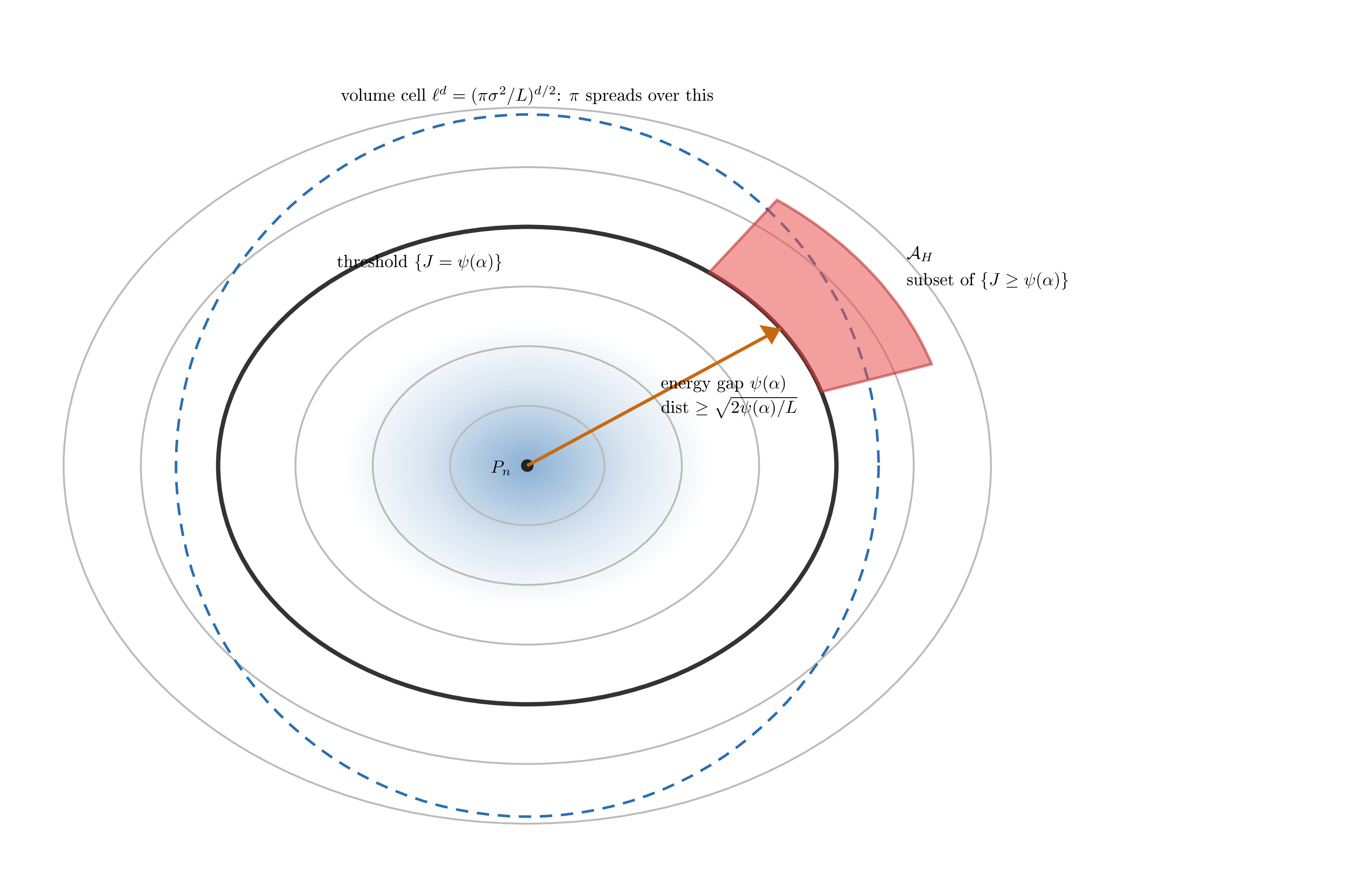
We take \[\mathcal{A}_H = \{Q \in \mathbb{R}^d : a_H(Q) > \alpha\}\] for a measurable alarm function \(a_H \ge 0\) with \(a_H(P_n) = 0\), and we assume a monotone link to the loss, \[J(Q) \;\ge\; \psi(a_H(Q)),\] for a strictly increasing \(\psi: [0,\infty) \to [0,\infty)\) with \(\psi(0) = 0\). By monotonicity \(\mathcal{A}_H \subseteq \{J \ge \psi(\alpha)\}\): triggering the alarm costs at least \(\psi(\alpha)\) in loss. This energy gap is what makes \(\mathcal{A}_H\) rare under \(\pi\).

Chi-squared divergence of the start.↩︎

When the initial law matters we record \[\chi_0^2 \;:=\; \chi^2(\nu_0 \,\|\, \pi) \;=\; \int \left(\frac{\nu_0}{\pi} - 1\right)^2 d\pi \;=\; \int \frac{\nu_0^2}{\pi}\, dQ - 1.\]

4 Static mass bound: probability at the end of training↩︎

The stationary measure \(\pi\) describes \(Q_T\) for \(T\) large, so \(\pi(\mathcal{A}_H)\) is the probability of ending training inside the failure region. We show it is exponentially small in \(d\). The mechanism is dimensional: \(\pi\) spreads over a large volume, and the rare, high-loss set \(\mathcal{A}_H\) captures exponentially little of it. This section uses only \(L\)-smoothness and a volume bound on \(\mathcal{A}_H\).

Dimensionless variables.↩︎

Define the natural length scale, the dimensionless energy variable, and the dimensionless gap \[\ell^2 \;:=\; \frac{\pi\sigma^2}{L}, \qquad s \;:=\; \frac{2 t}{\sigma^2}, \qquad \hat{\alpha} \;:=\; \frac{2 \psi(\alpha)}{\sigma^2}.\]

Sublevel-volume bound.↩︎

Let \(V(t) := \big|\{Q \in \mathcal{A}_H : J(Q) \le t\}\big|\) be the Lebesgue volume of the part of \(\mathcal{A}_H\) below loss level \(t\). Assume \(V(t) \le \Phi(t)\) for some non-decreasing \(\Phi\) with \(\Phi(t) = 0\) for \(t < \psi(\alpha)\), and set the dimensionless sublevel volume \[\hat{\Phi}(s) \;:=\; \Phi(s\sigma^2/2)\,\big/\,\ell^d,\] normalized by the volume cell \(\ell^d\). It satisfies \(\hat{\Phi}(s) = 0\) for \(s < \hat{\alpha}\).

4.1 The small-\(\sigma\) (Arrhenius) regime and the combined bound↩︎

2 is informative only when \(\pi\sigma^2 > L\), that is, when the noise is large or the dimension high. In the opposite regime a complementary barrier argument applies, using strong convexity. Since \(\pi\) is \((2m/\sigma^2)\)-strongly log-concave it has Gaussian tails of width \(\sigma/\sqrt{m}\) around \(P_n\), while smoothness places \(\mathcal{A}_H\) at radius at least \(\sqrt{2\psi(\alpha)/L}\) from \(P_n\). Gaussian concentration then gives, when \(\psi(\alpha) > dL\sigma^2/(4m)\), \[\pi(\mathcal{A}_H) \;\lesssim\; \exp\!\left(-\frac{2(m/L)\,\psi(\alpha)}{\sigma^2}\right),\] the bare Arrhenius rate \(2\psi(\alpha)/\sigma^2\) shaved by the condition number \(m/L \in (0,1]\). Folding the two bounds together through \(\min(e^{-a}, e^{-b}) = e^{-\max(a,b)}\) and defining the effective dimensional rate \[A_{\mathrm{eff}} \;:=\; \max\!\left(A,\;\; \frac{4m\,\psi(\alpha)}{L\,d\,\sigma^2}\right),\] gives the combined static bound \[\pi(\mathcal{A}_H) \leq e^{-A_{\mathrm{eff}}\, d/2}.\] In the large-\(\sigma\) or large-\(d\) regime, \(A_{\mathrm{eff}} = A\) and spreading does the work. In the small-\(\sigma\) regime \(\sigma^2 \ll 4m\psi(\alpha)/(dL)\), \(A_{\mathrm{eff}}\, d/2 = 2m\psi(\alpha)/(L\sigma^2)\) and the energy barrier does the work. The two regimes meet at the crossover \(Ad/2 \approx 2m\psi(\alpha)/(L\sigma^2)\), where the bound is least tight, and this crossover coincides with the burn-in scale of Section 5.

5 Dynamic mass control along the trajectory↩︎

The static bound is a statement at stationarity (\(t \to \infty\)). For finite \(t\) we control \(\nu_t(\mathcal{A}_H) = \mathbb{P}(Q_t \in \mathcal{A}_H)\) directly. The main result of this section assumes only the total mass \(\pi(\mathcal{A}_H)\), together with strong convexity and a finite initial chi-squared divergence. It is the dimension-free, shape-free bound. Its one weakness, a transient window in which it is uninformative, is exactly the swelling phenomenon of the introduction, and it is shortened in Section 6 by adding geometric information.

5.1 The common machinery↩︎

All bounds in this section and the next track the density ratio \[u_t := \frac{\nu_t}{\pi}.\] Substituting \(\nu_t = u_t \pi\) into 1 and using the identity \(\nabla \pi = -\frac{2}{\sigma^2}\, \pi\, \nabla J\) (the chain rule applied to \(\pi \propto e^{-2J/\sigma^2}\)), the time-independent factors cancel and \(u_t\) solves the backward Kolmogorov equation \[\partial_t u_t = \mathcal{L} u_t, \qquad \mathcal{L} = \frac{\sigma^2}{2}\,\Delta - \nabla J \cdot \nabla,\] where \(\mathcal{L}\) is the Langevin generator. Integration by parts against \(\pi\) shows \(\mathcal{L}\) is self-adjoint in \(L^2(\pi)\) with Dirichlet form \[\mathcal{E}(f) \;=\; -\langle f, \mathcal{L} f\rangle_\pi \;=\; \frac{\sigma^2}{2}\int |\nabla f|^2\, d\pi,\] and generates a conservative Markov semigroup \(P_t = e^{t\mathcal{L}}\) with \(P_t 1 = 1\). These are the standard generator, reversibility, and Dirichlet-form facts for the Langevin diffusion; see Pavliotis [10] and [11]. Every bound below converts a statement about \(u_t - 1\) into a statement about the set mass by pairing against the indicator \(\mathbf{1}_{\mathcal{A}_H}\).

5.2 The chi-squared spectral-gap bound↩︎

The centering device in Step 6 is the “warm-start” trick standard in the sampling literature ([19], [20], [6], [8]). The analytic-PDE route to the same \(L^2\) decay is in [17], [18], and a sampling-oriented exposition is in [9].

Explicit \(\chi_0^2\) for a Gaussian start.↩︎

The constant \(\chi_0^2\) is finite under mild conditions. If \(\nu_0 = N(P_n, \sigma_0^2 I)\) and \(m I \preceq \nabla^2 J \preceq L I\), then writing the requirement that the start be no wider than \(\pi\) allows, one has the closed-form envelope \[\chi_0^2 + 1 \;\le\; \left(\frac{\sigma_0^2}{s_-^2}\right)^{-d/2}\!\!\left(2 - \frac{\sigma_0^2}{s_+^2}\right)^{-d/2}, \qquad s_-^2 := \frac{\sigma^2}{2m},\;\; s_+^2 := \frac{\sigma^2}{2L},\] finite precisely when \(\sigma_0^2 < 2 s_+^2 = \sigma^2/L\). In particular \(\log \chi_0^2 = O(d)\), so \(\chi_0^2\) contributes at most an \(O(d)\) term to the burn-in below. (The clean Gaussian-Gaussian case \(J = \tfrac{a}{2}\|Q-P_n\|^2\) gives equality, and \(\chi_0^2 = 0\) when \(\sigma_0^2 = \sigma^2/(2a)\), i.e. the start equals \(\pi\).)

5.3 The maximum-principle ceiling↩︎

If the initial law has a bounded density ratio, a second, purely uniform-in-time bound is available, and it complements (\(\star\)) at small \(t\).

Combining 4 with Theorem 3, and using \(\|u_0 - 1\|_{L^2(\pi)}^2 \le \|u_0\|_\infty \int u_0\, d\pi - 1 = M - 1\), gives the two-sided sandwich with \(\sigma_t := \sqrt{(M-1)\,\pi(\mathcal{A}_H)(1-\pi(\mathcal{A}_H))}\,e^{-mt}\), \[\pi(\mathcal{A}_H) - \sigma_t \;\le\; \nu_t(\mathcal{A}_H) \;\le\; \min\!\Big(M\,\pi(\mathcal{A}_H),\;\; \pi(\mathcal{A}_H) + \sigma_t\Big).\] The two upper bounds cross at \(t_\star = \frac{1}{2m}\log\frac{1-\pi(\mathcal{A}_H)}{(M-1)\pi(\mathcal{A}_H)}\): the ceiling \(M\pi(\mathcal{A}_H)\) is tighter for \(t \le t_\star\), the relaxation bound for \(t \ge t_\star\). The ceiling requires \(M < \infty\), which fails for a point-mass start, and this failure is not cosmetic: it is exactly the case where swelling is real (Section 7).

5.4 Burn-in time and the combined safety bound↩︎

The bound (\(\star\)) is informative once its transient term is at most order one: \[\sqrt{\chi_0^2/\pi(\mathcal{A}_H)}\; e^{-mt} \;\le\; 1 \quad\Longleftrightarrow\quad t \;\ge\; \frac{1}{2m}\log\frac{\chi_0^2}{\pi(\mathcal{A}_H)}.\] Below this threshold the bound can exceed \(1\) and is vacuous; this is the swelling window. Substituting the static bound \(\pi(\mathcal{A}_H) \le K\, e^{-A d/2}\) from Theorem 2 gives the explicit burn-in time \[t_\star \;:=\; \frac{1}{2m}\log\frac{\chi_0^2}{K} \;+\; \frac{A}{4m}\, d.\] So \(t_\star\) grows linearly in \(d\) at rate \(A/(4m)\), plus a \(d\)-independent offset set by \(\chi_0^2\) and \(K\). For \(t \ge t_\star\), combining (\(\star\)) with the static bound gives the combined safety bound \[\mathbb{P}(Q_t \in \mathcal{A}_H) \;\le\; 2\,\pi(\mathcal{A}_H) \;\le\; 2 K\, e^{-A d/2},\] exponentially small in \(d\) at rate \(A/2\). In words: after a burn-in of order \(d\), the Langevin trajectory inherits the dimensionally suppressed safety of the stationary law.

6 Geometric isolation: shortening the burn-in↩︎

3 uses the global Poincaré constant \(m\) and only the total mass \(\pi(\mathcal{A}_H)\). It pays for this generality with the burn-in window, during which it cannot exclude swelling. The window is genuine for sets that lie on the transport path from \(\nu_0\) to \(\pi\) (Section 7), but for many failure regions of interest it is an artifact of discarding the geometry of \(\mathcal{A}_H\). This section restores that geometry through a local relaxation rate \(\lambda_{\mathcal{A}_H} \ge m\). The resulting bound relaxes at this faster, set-dependent rate, shortening the burn-in by the factor \(m/\lambda_{\mathcal{A}_H}\), and combined with the maximum-principle ceiling it caps the trajectory mass uniformly in time.

6.1 A pinned-down local relaxation rate↩︎

The informal idea is that mass cannot enter \(\mathcal{A}_H\) faster than it can cross the boundary \(\partial\mathcal{A}_H\), so a well-isolated set should relax faster than the global rate \(m\). Making this precise requires care, because the obvious candidate fails: the Rayleigh quotient of the centered indicator \(\phi_{\mathcal{A}_H} := \mathbf{1}_{\mathcal{A}_H} - \pi(\mathcal{A}_H)\) is \[\frac{\mathcal{E}(\phi_{\mathcal{A}_H})}{\operatorname{Var}_\pi(\phi_{\mathcal{A}_H})}, \qquad \mathcal{E}(\phi_{\mathcal{A}_H}) = \frac{\sigma^2}{2}\int |\nabla \mathbf{1}_{\mathcal{A}_H}|^2\, d\pi = +\infty,\] since \(\nabla \mathbf{1}_{\mathcal{A}_H}\) is the surface measure on \(\partial\mathcal{A}_H\). An indicator is not in the domain of the Dirichlet form, so a “restricted Poincaré constant” over step functions is vacuous. The right object is not the Dirichlet energy of the indicator but the rate at which the semigroup actually relaxes it.

Conductance as the geometric diagnostic.↩︎

The quantity that reads off isolation from the geometry of \(\mathcal{A}_H\) is the conductance under the Langevin diffusion, with diffusion coefficient \(\sigma^2/2\), \[h_{\mathcal{A}_H} \;:=\; \frac{\frac{\sigma^2}{2}\int_{\partial \mathcal{A}_H} \pi\, dS}{\min\big(\pi(\mathcal{A}_H),\, \pi(\mathcal{A}_H^c)\big)}.\] Say \(\mathcal{A}_H\) is flux-isolated if \(h_{\mathcal{A}_H}\) is bounded below independently of \(d\). A small conductance forces a slow-mode overlap and hence \(\lambda_{\mathcal{A}_H}\) close to \(m\), while for the isolated families of Section 6.3 one verifies \(\lambda_{\mathcal{A}_H} > m\) directly by symmetry or barrier comparison. We do not assert a universal one-line Cheeger lower bound \(\lambda_{\mathcal{A}_H} \ge h_{\mathcal{A}_H}^2/2\) for this spectral-measure quantity; the conductance is used as the geometric diagnostic, and the lower bound is established per family.

6.2 The flux-isolation theorem↩︎

This is 3 with the global rate \(m\) replaced by the local rate \(\lambda_{\mathcal{A}_H} \ge m\). For a flux-isolated set the burn-in time shrinks from \(\frac{1}{2m}\log(\chi_0^2/\pi(\mathcal{A}_H))\) to \(\frac{1}{2\lambda_{\mathcal{A}_H}}\log(\chi_0^2/\pi(\mathcal{A}_H))\), a saving by the factor \(m/\lambda_{\mathcal{A}_H}\), and the \(\min\) above caps the trajectory mass at \(M\pi(\mathcal{A}_H)\) for all \(t\), so no swelling above that ceiling ever occurs.

Remark (why not the linear prefactor).↩︎

The qualitatively stronger statement \(|\nu_t(\mathcal{A}_H) - \pi(\mathcal{A}_H)| \le (M-1)\pi(\mathcal{A}_H)\,e^{-\lambda_{\mathcal{A}_H} t}\), with prefactor linear in \(\pi(\mathcal{A}_H)\) and hence genuinely free of any burn-in, would follow from an \(L^1(\pi)\) contraction \(\|P_t \phi\|_{L^1(\pi)} \lesssim \|\phi\|_{L^1(\pi)} e^{-\lambda_{\mathcal{A}_H} t}\) paired against \(\|u_0 - 1\|_\infty \le M - 1\). The semigroup is an \(L^1(\pi)\) contraction but not at a positive rate in general; obtaining the exponential \(L^1\) rate requires hypercontractivity (available here from the Bakry-Émery log-Sobolev inequality) to lift \(L^1\) to \(L^2\) after a fixed lag, which yields the global log-Sobolev rate rather than the local rate \(\lambda_{\mathcal{A}_H}\). We therefore state the rigorous \(L^2\) bound and obtain the uniform-in-time control by intersecting it with the maximum-principle ceiling, as in the \(\min\) above.

Remark (the off-shell ball gains a factor).↩︎

For \(J(Q) = \tfrac{m}{2}\|Q\|^2\) the nonconstant eigenfunctions of \(-\mathcal{L}\) are Hermite polynomials, with the slowest modes (eigenvalue \(m\)) the linear coordinates \(Q_i\). For a ball centered at the mode, \(\mathcal{A}_H = \{\|Q\| < r\}\), symmetry gives \(\langle \phi_{\mathcal{A}_H}, Q_i\rangle_\pi = \int_{\mathcal{A}_H} Q_i\, d\pi = 0\) for every \(i\), so \(\phi_{\mathcal{A}_H}\) is orthogonal to the entire eigenvalue-\(m\) subspace and \(\lambda_{\mathcal{A}_H} \ge 2m\). A shell-slice, by contrast, has nonzero overlap with the linear modes, so \(\lambda_{\mathcal{A}_H} = m\) and 5 reduces to 3: no improvement, consistent with the swelling of Section 7.

6.3 High-dimensional taxonomy↩︎

The payoff of \(\lambda_{\mathcal{A}_H}\) is in the high-dimensional geometry of a strongly log-concave \(\pi\), where the mass concentrates on a thin shell. For the prototype \(J(Q) = \tfrac{1}{2}\|Q\|^2\) on \(\mathbb{R}^d\), \(\pi\) concentrates on \(\|Q\| \approx \sqrt{d}\) with \(O(1)\) width. Three families of small-\(\pi\)-mass failure regions behave very differently.

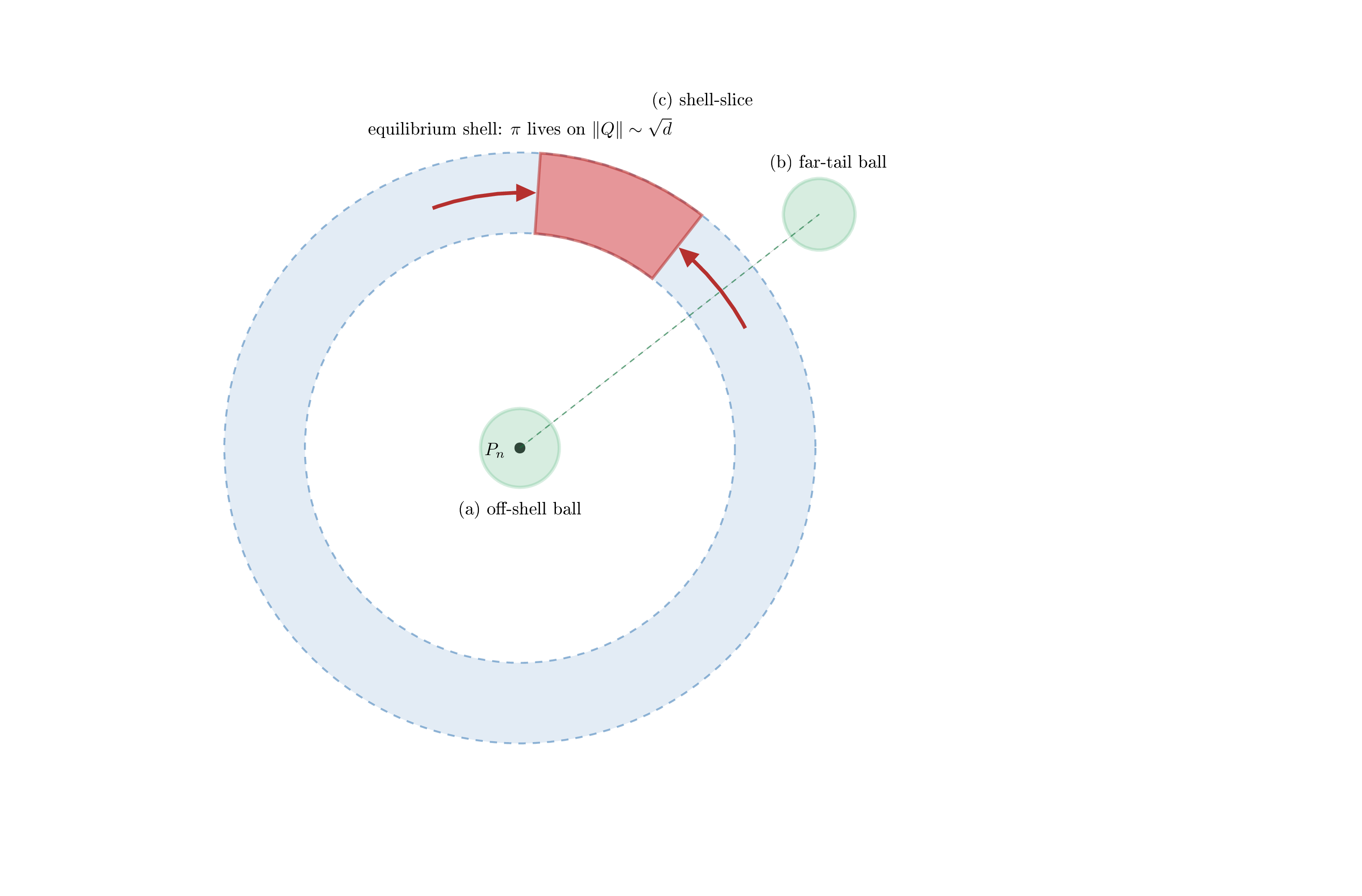
• Off-shell ball at the mode, \(\mathcal{A}_H = \{\|Q\| < r\}\) with \(r \ll \sqrt{d}\). The mode has lowest loss, but vanishing surface area faces the bulk: an entropic moat. Here \(\pi(\mathcal{A}_H) \sim e^{-d/2}\) while the boundary flux is comparably small, so \(h_{\mathcal{A}_H}\) and hence \(\lambda_{\mathcal{A}_H}\) are bounded below. Flux-isolated; 5 applies.

• Far-tail ball, \(\mathcal{A}_H = \{\|Q - Q_0\| < r\}\) with \(\|Q_0\| \gg \sqrt{d}\). A genuine energy barrier of height \(\sim \|Q_0\|^2/2\): hitting times grow exponentially (Eyring-Kramers) and \(\lambda_{\mathcal{A}_H}\) inherits the barrier-induced gap. Flux-isolated; 5 applies.

• Thin shell-slice, an angular wedge of the equilibrium shell \(\|Q\| \approx \sqrt{d}\). Equilibrium mass is small, but mass transports freely along the shell with no barrier, so \(h_{\mathcal{A}_H} \to 0\) and \(\lambda_{\mathcal{A}_H} \to 0\). Not flux-isolated; 5 is vacuous and only the ceiling \(M\pi(\mathcal{A}_H)\) survives.

The slogan: \(\pi(\mathcal{A}_H)\) small is not enough to keep \(\nu_t(\mathcal{A}_H)\) small for all \(t\); one also needs \(\lambda_{\mathcal{A}_H}\) bounded below. The shell-slice is the high-dimensional version of the swelling example, quantified next.

7 Sharpness and worked example: Ornstein-Uhlenbeck and the shell↩︎

This section makes the swelling phenomenon quantitative for the exactly solvable Ornstein-Uhlenbeck (OU) case. It shows that the burn-in window of Section 5 and the flux-isolation hypothesis of Section 6 are both necessary, and it exhibits the precise geometry, an angular slice of the equilibrium shell, where the transient overshoot is exponential in \(d\).

Take the quadratic loss \(J(Q) = \tfrac{1}{2}\sum_i \lambda_i Q_i^2\) with \(0 < \lambda_1 \le \cdots \le \lambda_d\), so the dynamics decouples into coordinatewise OU processes and \(\pi = N(0, \Sigma)\) with \(\Sigma = \operatorname{diag}(\sigma^2/(2\lambda_i))\). Start from an isotropic Gaussian \(\nu_0 = N(0, \sigma_0^2 I)\). Two quantities organize the analysis: the transient overshoot factor \[C_{\mathrm{bad}} \;:=\; \frac{\nu_{t_\star}(\mathcal{A}_H)}{\nu_0(\mathcal{A}_H)}\] at the worst time \(t_\star\), and the absolute mass \(\nu_t(\mathcal{A}_H)\) itself.

7.1 Isotropic case↩︎

Let \(J(Q) = \tfrac{a}{2}\|Q\|^2\) and let \(\mathcal{A}_H\) be confined to a level-set shell at radius \(B^\star\). With the single dimensionless ratio \[u \;:=\; \frac{(B^\star)^2}{d\,\sigma_0^2} \qquad \text{(squared shell radius over squared initial typical radius),}\] a direct Gaussian computation gives \[C_{\mathrm{bad}} \;=\; \exp\!\left[\frac{d}{2}\,\phi(u)\right], \qquad \phi(u) := u - 1 - \log u \;\ge\; 0,\] with equality \(\phi(u) = 0\) only at \(u = 1\). So the overshoot is exponential in \(d\) at rate \(\tfrac12\phi(u)\) whenever the shell radius is mismatched to the initial scale. This is the high-dimensional swelling: a set of tiny mass can gain an \(e^{\Theta(d)}\) factor in transit. The saving grace in the isotropic case is that \(\nu_t\) stays isotropic, so its mass on any shell set is bounded by the angular fraction of the shell, \[\nu_t(\mathcal{A}_H) \;\le\; R_{\mathrm{shell}} \qquad \text{(angular fraction of \mathcal{A}_H on S^{d-1}).}\] If \(R_{\mathrm{shell}}\) is itself exponentially small in \(d\), the overshoot is absorbed before it reaches absolute mass. This is exactly the dichotomy of Section 6: the shell-slice has small \(\pi(\mathcal{A}_H)\) (equilibrium reason) but is not flux-isolated (transit reason), so the burn-in window is real and \(C_{\mathrm{bad}}\) measures its depth.

7.2 Anisotropic case↩︎

With distinct \(\lambda_i\), the coordinates run at rates \(2\lambda_i\). Writing \(\rho_{0,i} = \lambda_i \sigma_0^2\) and the per-coordinate ratios \(u_i = Q_{0,i}^2/\sigma_0^2\), the overshoot factors out: \[C_{\mathrm{bad}} \;\le\; \exp\!\left[\frac{1}{2}\sum_{i=1}^d \phi(u_i)\right].\] Equality requires the per-coordinate peak times to align, which generically fails once the \(\lambda_i\) spread, so the effective dimension \(d_{\mathrm{eff}} = \#\{i : u_i \text{ far from } 1\}\) is governed by the geometry of \(\mathcal{A}_H\) relative to the initial scale. Anisotropy also destroys the uniform angular density, weakening the angular bound to \[\nu_t(\mathcal{A}_H) \;\le\; R_{\mathrm{shell}} \cdot \prod_{i=1}^d \frac{\sigma_{\max}(t)}{\sigma_i(t)},\] where \(\sigma_i(t)\) is the time-\(t\) standard deviation in coordinate \(i\). The prefactor is \(1\) at \(t = 0\) and grows to \(\prod_i \sqrt{\lambda_i/\lambda_1}\) as \(t \to \infty\), exponential in \(d\) for a spread spectrum.

7.3 Bounded condition number↩︎

The clean controllable case is a bounded condition number \(K := \lambda_d/\lambda_1\) together with an initial scale chosen in range, \(\sigma_0^2 \in [1/\lambda_d,\, 1/\lambda_1]\) (in the \(\sigma = \sqrt{2}\) normalization). Then \(\sigma_i^2(t)\) stays in \([1/\lambda_d, 1/\lambda_1]\) for all \(i\) and \(t\), so \(\sigma_{\max}/\sigma_i \le \sqrt{K}\) and the angular bound becomes uniform in time, \[\nu_t(\mathcal{A}_H) \;\le\; R_{\mathrm{shell}} \cdot K^{d/2} \qquad \text{for all } t \ge 0.\] Three regimes: \(K = 1\) recovers the isotropic bound; \(K - 1 = O(1/d)\) keeps \(K^{d/2} = O(1)\); a fixed \(K > 1\) gives exponential growth at rate \(\tfrac12\log K\). The bound is useful when \(R_{\mathrm{shell}}\) decays faster than \(K^{d/2}\) grows, that is for \(\mathcal{A}_H\) of angular radius below \(\arcsin(1/\sqrt{K})\) on \(S^{d-1}\).

7.4 Combined statement and where dimension enters↩︎

Putting the transit and angular bounds together, \[\nu_t(\mathcal{A}_H) \;\le\; \min\!\Big(\, C_{\mathrm{bad}}\cdot \nu_0(\mathcal{A}_H),\;\; R_{\mathrm{shell}}\cdot \textstyle\prod_i \sigma_{\max}(t)/\sigma_i(t)\,\Big).\] Two independent sources of exponential-in-\(d\) growth appear: the overshoot \(C_{\mathrm{bad}} = \exp[\tfrac12\sum_i \phi(u_i)]\), controlled by the geometry of \(\mathcal{A}_H\) through the \(u_i\); and the angular amplification \(\prod_i \sigma_{\max}/\sigma_i \le K^{d/2}\), controlled by the spectral spread of \(J\). Avoiding both requires either placing \(\mathcal{A}_H\) in a low-\(d_{\mathrm{eff}}\) subspace with the initial law matched to stationarity in the complementary directions, or a bounded \(K\) with \(\sigma_0\) in range and \(\mathcal{A}_H\) angularly thin. This is the constructive counterpart of the flux-isolation hypothesis of 5.

7.5 The one-dimensional swelling example↩︎

The simplest instance, recovering the introduction: \(J(Q) = Q^2/2\) on \(\mathbb{R}\) with \(\sigma^2 = 2\), so \(\pi = N(0,1)\) and \(m = 1\). Start at \(\nu_0 = \delta_{10}\) and take \(\mathcal{A}_H = [4,6]\). Then \(\nu_0(\mathcal{A}_H) = 0\), \(\pi(\mathcal{A}_H) \approx 10^{-5}\), but \(\nu_t = N(10 e^{-t}, 1 - e^{-2t})\), so at \(t = \log 2\) the law is \(N(5, 3/4)\) and \(\nu_t(\mathcal{A}_H) \approx 0.7\), an overshoot of about \(10^5\). Here \(M = \infty\) (point mass), so the ceiling 4 is vacuous, and \(\mathcal{A}_H\) is the one-dimensional analogue of a shell-slice on the transport path, so \(\lambda_{\mathcal{A}_H}\) is not bounded below and 5 does not apply. Both protective hypotheses fail at once, which is why this is the canonical demonstration that strong convexity controls the relaxation rate but not the transient peak.

8 Summary↩︎

The picture has three layers. At stationarity, the failure region has exponentially-small-in-\(d\) mass, \(\pi(\mathcal{A}_H) \le K e^{-Ad/2}\) (2), with a complementary Arrhenius rate in the small-noise regime. Along the trajectory, a shape-free bound (3) relaxes to twice this static mass after a burn-in of order \(d\), using only the total mass and the global gap \(m\). Adding geometric information, a local relaxation rate \(\lambda_{\mathcal{A}_H} \ge m\) (Definition 1, 5) replaces the global rate by a faster set-dependent one for flux-isolated sets, shortening the burn-in by the factor \(m/\lambda_{\mathcal{A}_H}\); combined with the maximum-principle ceiling it caps the trajectory mass uniformly in time.

The two grades of dynamic bound are the two ends of one tradeoff. Total-mass control is universal and dimension-free but transiently uninformative; shape-aware control shortens the transient and, via the ceiling, caps the mass uniformly, but requires verifying that \(\mathcal{A}_H\) is geometrically isolated and that the start has a bounded density ratio. The worked OU example (Section 7) shows the gap between them is real: an angular shell-slice has tiny equilibrium mass yet an \(e^{\Theta(d)}\) transient overshoot, and only the flux-isolation hypothesis rules it out. Strong convexity sets the relaxation rate; the geometry of \(\mathcal{A}_H\) decides whether there is a bulge before relaxation wins.

References↩︎