Fast Rates for Semi-Supervised Learning via
Data-Augmentation Graph Regularization
July 08, 2026
Abstract
Self-supervised learning matches supervised accuracy from a fraction of the labels, but the labeled-sample efficiency behind this has lacked a theoretical explanation. We provide one. Data augmentation induces a similarity graph on the unlabeled data, so downstream learning on that graph is graph-Laplacian-regularized learning. We prove a fast transductive rate, \(O(1/n_L)\) in the number of labels, in place of the supervised \(O(1/\sqrt{n_L})\), by carrying the leave-one-out stability apparatus of Johnson and Zhang (JMLR 2007) over to the augmentation graph, and without the unrealistic assumptions of limit-based analyses (exact kernel, generalizing features). The bound makes augmentation quality explicit: the expected error is at most \(C/n_L + R_{\mathrm{DA}}(y)\), where the data-augmentation alignment error \(R_{\mathrm{DA}}(y)\) is the graph-cut mass of augmentations that cross a label boundary, so good augmentations let few labels suffice. The analysis uses a streamlined loss that drops the projector, negative-sample, and orthogonality overhead of standard objectives yet still recovers the top-\(K\) ideal features in the infinite-data limit, the augmentation-kernel eigenspace studied by Zhai et al. The result explains the observed accuracy-versus-label-count curve rather than only bounding a generalization gap.
semi-supervised learning, data augmentation, graph Laplacian regularization, algorithmic stability, fast rates
1 Introduction↩︎
Self-supervised learning matches supervised accuracy from a small fraction of the labels. SimCLR [1] matches a supervised ResNet-50 from a linear probe and is strong at \(1\%\) and \(10\%\) of ImageNet labels; SimCLRv2 [2] reaches \(80.9\%\) top-1 with only \(10\%\) of the labels, an order-of-magnitude label saving; and CPC v2 [3] named the “data-efficient” framing with two to five times fewer labels. This accuracy-versus-label-count curve is one of the most reported empirical facts about representation learning, yet it remains theoretically under-explained.
The feature-learning side of the story is by now well understood. Different self-supervised losses (spectral contrastive, contrastive and non-contrastive, kernel-PCA) all recover the leading eigenfunctions of the augmentation similarity kernel \(k^{\mathrm{DAF}}\). But that theory lives in the infinite-data limit: it characterizes the features a method would learn from unlimited unlabeled data, and says nothing about the finite labeled-sample behavior downstream, which is exactly what the curve above measures. Two assumptions used there are also unrealistic for the few-augmentation regime: that the expectation kernel is learned exactly, and that the factoring features generalize to unseen points.
This paper supplies the missing labeled-sample guarantee. The data augmentations define a similarity graph on the unlabeled data, so downstream learning on that graph is graph-Laplacian-regularized learning. For that setting a transductive fast rate is already available: [4] bound the transductive error of Laplacian-regularized multi-class graph learning by leave-one-out algorithmic stability and obtain an \(O(1/n)\) rate in the labeled count under balanced components, governed by a learning-theoretic graph cut. Our rate results (Theorems 2 and 3) are that apparatus, specialized and reinterpreted for the augmentation graph; the contribution is not a new rate mechanism but its placement. Read on the augmentation graph, the cut becomes an augmentation-quality term \(R_{\mathrm{DA}}(y)\), the number of graph components becomes a property of the augmentation distribution, and the bound turns into a statement about how few labels a good augmentation buys, in place of the supervised \(O(1/\sqrt{n_L})\). The applied companion to this work (the NeurIPS 2024 paper of Ghosh et al., showing \(2\times\) less pretraining data empirically) is the motivation on the pretraining axis; here we explain, with rates, why the downstream labeled-sample efficiency holds.
1.0.0.1 Contributions.
A fast transductive rate on the augmentation graph (Theorem 2). We carry the Johnson–Zhang leave-one-out stability apparatus over to the augmentation graph: an \(O(1/n_L)\) oracle inequality for labels propagating from the labeled set to the unlabeled nodes. We claim no novelty in the stability mechanism itself; the point is its setting. Relative to the feature-learning limit theory, the argument also avoids two unrealistic assumptions: it never requires the kernel to be learned exactly, and it bounds the error on the actual unlabeled sample rather than assuming features generalize.
Augmentation quality enters the bound (Theorem 3). The expected error is bounded by \(C/n_L + R_{\mathrm{DA}}(y)\), where the data-augmentation alignment error \(R_{\mathrm{DA}}(y)\) is the graph-cut mass of augmentations that cross a label boundary. This term explains accuracy: better augmentations shrink it, so fewer labels suffice.
A streamlined loss (Theorem 5). Dropping the projector-dimension, negative-sample, and orthogonality / non-collapse overhead (one label per class already prevents collapse) costs nothing in the limit: the streamlined loss is algorithmically stable and still recovers the top-\(K\) ideal features.
2 Setup and notation↩︎
We study vector classification on a data domain \(\mathcal{X}\subset\mathbb{R}^{d_0}\) with label set \(\mathcal{Y}=\{1,\dots,K\}\). A score function \(g:\mathcal{X}\to\mathbb{R}^K\) is followed by the argmax one-hot classifier; we write \(e_y\) for the one-hot vector of label \(y\). The training loss is a standard classification loss \(\ell(g,z)\), and for \(z=(x,y)\) we abbreviate \(\ell(g,z)=\ell(g(x),y)\).
Assumption 1 (\(\sigma\)-admissible loss). The loss \(\ell(\cdot,y)\) is convex in its first argument and \(\sigma_\ell\)-Lipschitz on a bounded domain \(D_\ell\): \[|\ell(f,y)-\ell(g,y)|\le \sigma_\ell\,\|f-g\|, \qquad \forall f,g\in D_\ell,\;\forall y\in\mathcal{Y}.\]
This holds for the standard score-based losses (cosine-similarity, cross-entropy on a bounded domain, regularized least squares); see Appendix 8.
2.0.0.1 Transductive data.
Let \(S^U=\{x_1,\dots,x_m\}\) be the unlabeled sample of \(m\) points. A subset of \(n_L\le m\) of them is labeled, giving \(S^L=\{z_1,\dots,z_{n_L}\}\) with \(z_j=(x_j,y_j)\); throughout, \(S^L\subset S^U\) (revealing a label does not add a point). The labeled training loss is \[L(g,S^L)=\frac{1}{n_L}\sum_{z_j\in S^L}\ell(g,z_j).\] The setting is transductive: error is measured on the unlabeled nodes of the fixed sample \(S^U\), not on a fresh draw.
2.1 The data-augmentation graph↩︎
Data augmentations are random maps \(M:\mathcal{X}\to\mathcal{X}\). Writing \(p(z\mid x_0)=\mathbb{P}\!\left(z=M(x_0)\right)\) for the probability of reaching \(z\) from a seed \(x_0\), the (forward) data-augmentation covariance kernel is \[\label{eq:kdaf} k^{\mathrm{DAF}}(x,z)=\mathbb{E}_{x_0\sim\rho_X}\!\left[\,p(x\mid x_0)\,p(z\mid x_0)\,\right],\tag{1}\] together with its symmetric degree-normalized version. Writing \(d(x)=\mathbb{E}_{z\sim\rho_X}\!\left[k^{\mathrm{DAF}}(x,z)\right]\) for the augmentation mass (degree) at \(x\), the normalized kernel is \[\label{eq:knorm} k(x,z)=\frac{k^{\mathrm{DAF}}(x,z)}{\sqrt{d(x)}\,\sqrt{d(z)}} .\tag{2}\] On the sample \(S^U\) this gives the weighted graph \(G=(S^U,W)\) with raw weights \(w_{ij}=k^{\mathrm{DAF}}(x_i,x_j)\ge 0\), degrees \(\mathbf{S}_j=\deg_j(G)=\sum_{j'}w_{j,j'}\), and normalized adjacency \(W=\mathbf{S}^{-1/2}\,[w_{ij}]\,\mathbf{S}^{-1/2}\), so that \(W_{ij}=k(x_i,x_j)\). Convolution against \(W\) realizes the integral operator \(T_K\) on \(\rho_X\): applied to features on \(S^U\), \(W f(S^U)=T_K f\), recovering the ideal RKHS picture in the large-sample limit. The degrees \(\mathbf{S}_j\) are exactly the scaling factors of the \(\mathbf{S}\)-normalized Laplacian used below. The symmetric normalization \(W=\mathbf{S}^{-1/2}[w_{ij}]\mathbf{S}^{-1/2}\) is the geometric mean of the two random-walk normalizations \(\mathbf{S}^{-1}[w_{ij}]\) and \([w_{ij}]\mathbf{S}^{-1}\), which encode the forward chain (augment a seed and ask where the view lands) and the backward chain (given a view, ask which seed produced it); the two are adjoint, share the spectrum of \(W\), and the data-augmentation error \(R_{\mathrm{DA}}(y)\) of Section 4 is measured in this symmetric normalization.
2.2 The regularizer and the combined objective↩︎
Let \(\mathbf{K}\in\mathbb{R}^{m\times m}\) be a symmetric positive-definite kernel matrix derived from the augmentation graph \(G\) (and from a fixed backbone \(f_0\)), so that \(\mathbf{K}\) depends on neither the labels nor the trained score \(g\). The quadratic regularizer penalizes each class score separately, \[\label{eq:reg} Q(g,S^U)=\sum_{k=1}^K g_{\cdot,k}^\top\,\mathbf{K}^{-1}\,g_{\cdot,k}, \qquad g_{\cdot,k}=(g_{1,k},\dots,g_{m,k})^\top .\tag{3}\] The graph realization (used in Section 4) takes \(\mathbf{K}^{-1}=\alpha\,\mathbf{S}^{-1}+\mathcal{L}_{\mathbf{S}}(G)\), where \(\mathcal{L}_{\mathbf{S}}(G)=\mathbf{S}^{-1/2}\mathcal{L}(G)\,\mathbf{S}^{-1/2}\) is the \(\mathbf{S}\)-normalized graph Laplacian and \(\alpha>0\) keeps \(\mathbf{K}\) strictly positive definite; then \[\label{eq:reg-graph} Q(g,S^U)=\sum_{k=1}^K\Big(\underbrace{\alpha\sum_j \mathbf{S}_j^{-1}g_{j,k}^2}_{\text{ridge}} +\underbrace{\tfrac12\sum_{j,j'}w_{j,j'}\big(\mathbf{S}_j^{-1/2}g_{j,k}-\mathbf{S}_{j'}^{-1/2}g_{j',k}\big)^2}_{\text{Laplacian energy}}\Big).\tag{4}\] The second term is the invariance-to-augmentation energy. It is a weighted sum of squared differences of the degree-normalized score across edges of the augmentation graph: an edge weight \(w_{j,j'}\) is large precisely when \(x_j\) and \(x_{j'}\) are likely to arise as augmentations of a common seed, so a small Laplacian energy means the score varies little between points the augmentations identify, i.e.the score is approximately invariant to data augmentation. This is the standard manifold / label-propagation prior: minimizing 4 pushes each class score toward functions that are smooth along the augmentation graph, while the ridge term contributes the \(\alpha\mathbf{S}^{-1}\) that keeps \(\mathbf{K}\) strictly positive definite and the regularizer proper. Evaluating this energy at the label indicator is exactly what yields the graph cut \(R_{\mathrm{DA}}(y)\) of Section 4, the channel through which augmentation quality enters the rate.
Definition 1 (SSL algorithm). Given \((S^L,S^U)\), the algorithm returns the regularized empirical minimizer \[\label{eq:alg} f=A(S^L,S^U)=\arg\min_{g}\;\Big\{\,L(g,S^L)+\lambda\,Q(g,S^U)\,\Big\}, \qquad \lambda>0 .\qquad{(1)}\]
Remark 1 (No collapse term needed). Because \(\mathbf{K}\) is built from the unlabeled graph and is independent of \(g\) and of the labels, the objective ?? carries no projector-dimension, negative-sample, or orthogonality/non-collapse penalty. With at least one label per class the supervised term already prevents feature collapse; this is the streamlined loss analyzed in Section 5.
3 A fast transductive rate via leave-one-out stability↩︎
The first result is an oracle inequality with a fast \(O(1/n_L)\) dependence on the number of labels. Error is measured by the semi-supervised leave-one-out loss: move one labeled point to the unlabeled set, retrain, and evaluate on the held-out point, averaged over the training set.
Definition 2 (Leave-one-out loss). For \(f^{\backslash j}=A(S^L\setminus z_j,\,S^U)\), \[L_{\mathrm{loo}}(A,S^L,S^U)=\frac{1}{n_L}\sum_{z_j\in S^L}\ell\!\left(f^{\backslash j},z_j\right).\]
The argument rests on a one-point stability bound for the algorithm ?? : removing a labeled point perturbs the fitted score at that point by only \(O(1/(\lambda n_L))\).
Lemma 1 (Uniform stability). Under Assumption 1, with \(\mathbf{K}\) symmetric positive definite and \(f\), \(f^{\backslash i}\) defined by ?? , for every \(i\) \[\left|f(x_i)-f^{\backslash i}(x_i)\right|\;\le\;\frac{\sigma_\ell\,\mathbf{K}_{i,i}}{2\,\lambda\,n_L}.\]
Theorem 2 (Transductive oracle inequality). Consider the algorithm ?? under Assumption 1. Then, in expectation over the i.i.d.choice of which \(n_L\) of the \(m\) nodes are labeled, \[\label{eq:oracle} \mathbb{E}_{S^L}\!\left[L_{\mathrm{loo}}(A,S^L,S^U)\right] \;\le\; \underbrace{\min_{g}\Big\{\tfrac{1}{m}\textstyle\sum_{i=1}^m\ell(g,z_i)+\lambda\,Q(g,S^U)\Big\}}_{\text{full-label regularized oracle}} \;+\; \frac{\sigma_\ell^2}{2\,\lambda\,n_L}\cdot\frac{1}{m}\sum_{i=1}^m \mathbf{K}_{i,i}.\qquad{(2)}\]
3.0.0.1 Reading the bound.
The first term is the regularized risk one would obtain from labeling all \(m\) nodes, so ?? is a genuine oracle inequality. The second term is the price of having only \(n_L\) labels. With \(\lambda\) fixed and the graph kernel normalized so that \(\frac{1}{m}\sum_i\mathbf{K}_{i,i}\) is bounded, that price is \(O(1/n_L)\), the improvement over the supervised \(O(1/\sqrt{n_L})\) rate. The gain is transductive: it concerns label propagation across the fixed unlabeled sample, not generalization to a fresh draw. (The same stability constant also yields a high-probability \(O(1/\sqrt{n_L})\) generalization-gap bound through Bousquet and Elisseeff; the fast rate above is the transductive, in-expectation statement.)
3.0.0.2 Proof idea.
Lemma 1 follows by comparing the minimizers \(f\) and \(f^{\backslash i}\) through the Bregman divergence of \(R_r(g)=L(g,S^L)+\lambda Q(g,S^U)\): the divergence telescopes to a single loss difference, \(\sigma\)-admissibility bounds that difference by \(\sigma_\ell|\Delta f(x_i)|\), and the Cauchy–Schwarz inequality \(f_i^2\le Q(f)\,\mathbf{K}_{i,i}\) closes the loop. Feeding the lemma into \(\ell(f^{\backslash i},z_i)\le\ell(f,z_i) +\sigma_\ell|f(x_i)-f^{\backslash i}(x_i)|\), averaging over \(S^L\), adding the regularizer, using minimality of \(f\) to swap in an arbitrary \(g\), and taking expectations gives ?? . The full proof is in Appendix 8.
4 Augmentation quality controls the error↩︎
Theorem 2 bounds the loss by a regularized oracle term that still depends on the augmentation graph. We now evaluate that term to expose what makes it small: the degree to which the augmentations respect the labels. Specializing the regularizer to the graph form \(\mathbf{K}^{-1}=\alpha\,\mathbf{S}^{-1}+\mathcal{L}_{\mathbf{S}}(G)\) from Section 2, the oracle term is controlled by a single graph-cut quantity.
Definition 3 (Data-augmentation alignment error). Partition the edges of \(G\) by whether they cross a label boundary, into different, \(D\), and same, \(S\), \[D=\{(j,j'):y_j\neq y_{j'}\},\qquad S=\{(j,j'):y_j=y_{j'}\},\] and define the \(\mathbf{S}\)-normalized cut of the labeling \(y\), \[\label{eq:cut} \operatorname{cut}(\mathcal{L}_{\mathbf{S}},y) =\sum_{(j,j')\in D}\frac{w_{j,j'}}{2}\!\left(\frac{1}{\mathbf{S}_j}+\frac{1}{\mathbf{S}_{j'}}\right) +\sum_{(j,j')\in S}\frac{w_{j,j'}}{2}\!\left(\frac{1}{\sqrt{\mathbf{S}_j}}-\frac{1}{\sqrt{\mathbf{S}_{j'}}}\right)^{2}.\qquad{(3)}\] The data-augmentation alignment error \(R_{\mathrm{DA}}(y)\) is the normalization of ?? : the mass, under the augmentation-graph edge weights, of pairs whose augmentations cross a label boundary. It is zero exactly when augmentations never mix labels.
Assumption 2 (Balanced components and bounded margin). Two conditions, distinct in role. (i) Balanced components: in the near-zero-cut regime the augmentation graph splits into \(q\) pure components (maximal label-consistent connected pieces) of sizes \(m_1\le\cdots\le m_q\) whose smallest is a \(\Theta(1/q)\) fraction of the whole, so that \(m/m_1=\Theta(q)\). (ii) Bounded margin: the margin constant \(c\) of the admissible loss (the separation in Assumption 1 between the regions where \(\phi_0(\cdot,1)\) and \(\phi_0(\cdot,0)\) are small) is bounded below by a universal constant, uniformly in \(m\).
The two conditions do different work. Component balance is what upgrades the graph-cut bound from the slow \(n_L^{-1/2}\) behavior to the fast \(n_L^{-1}\) rate: the Johnson–Zhang fast bound carries a factor \(m/m_1\ge q\) (their Theorem 5, [4]), which collapses to \(\Theta(q)\) exactly when the components are balanced and otherwise degrades the rate back toward \(\sqrt{q/n_L}\). The margin bound is a separate requirement, present at every rate: it keeps the surrogate-to-\(0/1\) conversion constant \(b/(ac)\) from growing as the sample does. (Ordinary class balance, each label on a \(\Theta(1/K)\) fraction of nodes, is a third and distinct condition and is not what produces the fast rate.)
Theorem 3 (Expected loss in terms of the DA error). Consider the algorithm ?? with the graph kernel \(\mathbf{K}^{-1}=\alpha\,\mathbf{S}^{-1}+\mathcal{L}_{\mathbf{S}}(G)\) under Assumptions 1 and 2. Then there is a sample-independent choice of \(\lambda\) for which the expected transductive classification error obeys \[\label{eq:daerror} \mathbb{E}_{S^L}\!\left[\operatorname{err}\right] \;\le\; \frac{C}{n_L}\;+\;R_{\mathrm{DA}}(y),\qquad{(4)}\] with \(C=C(\sigma_\ell,\alpha,\operatorname{tr}\mathbf{K})\) independent of \(n_L\) but carrying the component-balance factor \(m/m_1\ge q\) of Assumption 2: under balance \(C=\Theta(q)\), and without it \(C\) grows with \(m/m_1\) and the rate degrades toward \(\sqrt{q/n_L}\). In particular, if the augmentation is perfectly label-consistent then \(R_{\mathrm{DA}}(y)=0\) and the error is \(O(q/n_L)\), fast in the label count \(n_L\).
4.0.0.1 Why this term explains accuracy.
Unlike a generalization-gap bound, ?? bounds the error itself, and it factorizes the two things a practitioner controls: more labels shrink \(C/n_L\), while better augmentations shrink \(R_{\mathrm{DA}}(y)\). Good augmentations therefore let few labels suffice, which is the accuracy-versus-label-count behavior reported for SimCLR and SimCLRv2 (Section 1). The quantity \(R_{\mathrm{DA}}(y)\) is, in isolation, essentially the class-boundary edge mass \(\alpha\) of HaoChen et al.(2021); the contribution here is that it enters a transductive, fast-rate labeled-sample bound through the graph cut and stability, rather than a slow Rademacher bound in unlabeled samples.
4.0.0.2 Proof idea.
Insert the label indicator \(f_{j,k}=\delta_{y_j,k}\) into the oracle term of Theorem 2: the supervised loss vanishes and the regularizer evaluates to \(\lambda\big(\alpha s+\operatorname{cut}(\mathcal{L}_{\mathbf{S}},y)\big)\) with \(s=\sum_j \mathbf{S}_j^{-1}\), so the oracle term is the graph cut \(R_{\mathrm{DA}}(y)\). Optimizing \(\lambda\) in the Johnson–Zhang bound and taking its fast, balanced-component regime turns the in-expectation stability term of Theorem 2 into the \(C/n_L\) price, with \(C\) carrying the \(m/m_1\) factor controlled by Assumption 2(i); the margin bound of Assumption 2(ii) then supplies the constant that passes the surrogate loss to the \(0/1\) classification error without a sample-dependent constant. The full argument, with the explicit constant deferred to [4], is in Appendix 8.
Remark 4 (Multiplicative versus additive form). Tracking the cut through the optimization of [4] in fact gives the slightly tighter multiplicative* statement \(\mathbb{E}_{S^L}[\operatorname{err}]\le \tfrac{C}{n_L}\big(1+R_{\mathrm{DA}}(y)\big)\), of which the additive form ?? is the immediate corollary (since \(R_{\mathrm{DA}}(y)/n_L\le R_{\mathrm{DA}}(y)\)). We state the additive form as the headline because it cleanly separates the two levers a practitioner controls, the label budget \(n_L\) and the augmentation quality \(R_{\mathrm{DA}}(y)\). The two forms make qualitatively different asymptotic predictions, and the controlled experiment of Section 7.1, where \(\lambda/a\) and the cut are known exactly, shows the resolution is loss-dependent. The admissible surrogate the algorithm actually minimizes carries an additive floor that grows linearly with \(\operatorname{cut}(\mathcal{L}_{\mathbf{S}},y)\) through the origin, with slope at most \(\lambda/a\), exactly as ?? predicts. The downstream \(0/1\) classification error, by contrast, shows no persistent floor and keeps descending with \(n_L\), the behaviour the multiplicative form describes. The additive \(R_{\mathrm{DA}}\) floor is thus a property of the surrogate the bound is proved for; it acts on the classification error as a soft, label-budget-dependent penalty rather than a hard ceiling.*
5 The infinite-data limit recovers the ideal features↩︎
The previous sections fix the backbone and analyze the labeled-sample behavior of the linear score on the augmentation graph. The last result closes the loop with the feature-learning literature: the streamlined loss of Section 2 loses nothing in the limit. As the unlabeled sample grows and the augmentation graph converges to the integral operator \(T_K\) of the kernel \(k^{\mathrm{DAF}}\) 1 on \(\rho_X\), its minimizers recover the same ideal features that contrastive and non-contrastive objectives recover.
Assumption 3 (Spectral gap). The integral operator \(T_K\) of \(k^{\mathrm{DAF}}\) on \(\rho_X\) has a positive gap after the \(K\)-th eigenvalue: ordering its eigenvalues \(\mu_1\ge\mu_2\ge\cdots\), the gap \(\gamma_K=\mu_K-\mu_{K+1}>0\).
Theorem 5 (Limit features). Suppose the augmentation alignment error vanishes, \(R_{\mathrm{DA}}(y)=0\), and let Assumption 3 hold. As \(m\to\infty\) the normalized graph operator \(W\) converges to \(T_K\) on \(\rho_X\), and the minimizer of the streamlined loss ?? converges to a map whose span equals the top-\(K\) eigenspace of \(T_K\), i.e.the leading \(K\) Mercer eigenfunctions of \(k^{\mathrm{DAF}}\). The convergence of the learned subspace to the ideal one is at rate \(O\!\big(1/(\gamma_K\sqrt{m})\big)\).
Remark 6 (Relation to existing equivalences). Theorem 5 is not a new object: the same top-\(K\) spectral target is recovered by the spectral contrastive loss [5], by contrastive and non-contrastive losses read as global and local spectral embedding [6], and, most generally, by the context/expectation operator of [7]. We restate it as a consequence* of the streamlined formulation to show that dropping the projector-dimension, negative-sample, and orthogonality/non-collapse overhead costs nothing in the limit. The contribution of this paper is the finite labeled-sample rate of Sections 3–4, which the limit theory does not provide.*
5.0.0.1 Proof idea.
With \(R_{\mathrm{DA}}(y)=0\) the supervised term selects the class-consistent directions and the Laplacian energy \(Q(\cdot,S^U)\) orders them by the spectrum of \(W\), so the minimizer’s span is the top-\(K\) eigenspace of \(W\). Two classical tools then transfer this to \(T_K\): an empirical-operator concentration bound \(\|W-T_K\|=O_P(1/\sqrt m)\) [8], and the Davis–Kahan \(\sin\Theta\) theorem [9], which converts the operator gap \(\gamma_K\) into control of the angle between the two top-\(K\) eigenspaces. The self-contained argument is in Appendix 8.
6 Related work↩︎
6.1 The operator and spectral view of SSL↩︎
A now-standard view holds that the various self-supervised objectives all recover the leading eigenfunctions of an operator induced by the augmentation distribution, so that the apparent diversity of losses is largely cosmetic. [5] established the canonical case: the spectral contrastive loss recovers the leading eigenvectors of the augmentation graph. [6] unified contrastive and non-contrastive methods under a single spectral-embedding lens, with contrastive objectives implementing a global spectral embedding and VICReg- or Barlow-style objectives a local one. [10] characterized the eigenfunctions of the positive-pair Markov chain as the output of kernel PCA, the optimal basis for approximately view-invariant functions. [11] recast pretraining as RKHS approximation and regression, with SSL approximating the top-\(d\) eigenspace of the augmentation-induced kernel, and turn this picture into two model-complexity-free generalization bounds for the linear probe, decomposing its error into an RKHS-regression estimation term and an RKHS-approximation term and comparing augmentations through an augmentation complexity. The most general statement to date is the Contextures framework [7], in which supervised, self-supervised, and manifold learning all recover the top-\(d\) singular functions of a common context operator. We take this operator view as background: our streamlined loss recovers the top-\(K\) ideal features in the infinite-data limit, which is a consequence of this line of work rather than a new equivalence. Our contribution is not another characterization of the limit but a finite-sample guarantee in the number of labels.
6.2 Generalization rates for SSL and semi-supervised learning↩︎
The downstream generalization of representation learning was first bounded by [12], whose latent-class analysis gives a slow \(O(1/\sqrt{M})\) rate in the number \(M\) of unlabeled pairs. [13] sharpened this line, removing the dependence on the number of negatives and obtaining optimistic bounds that imply fast \(O(1/n)\) behaviour under a low-noise condition; their \(n\), however, counts unlabeled contrastive tuples rather than labels, and the bound is not transductive. Fast rates in the number of labeled samples are classically available only under strong distributional assumptions: [14] obtains them under the cluster assumption and [15] under a parametric model, both inductively and without an augmentation graph. On the negative side, [16] give lower bounds that delimit when unlabeled data can help at all. A generic transductive baseline is that of [17], whose information-theoretic bounds for transductive learning are of the standard slow \(O(1/\sqrt{n})\) order. A fast transductive \(O(1/n)\) labeled-sample rate is, however, already available for graph-Laplacian learning: it is precisely the result of [4] (see the graph-SSL subsection below), on which our rate theorems are built. What is not yet available, and what we supply, is that rate carried onto the augmentation graph, so that the governing quantity is augmentation quality rather than a generic cut and the label-efficiency of self-supervised learning becomes the object bounded, all without a density or parametric assumption.
6.3 Stability-based generalization↩︎
Our analysis routes through algorithmic stability rather than the Rademacher-complexity machinery that is standard in the contrastive literature. The template is that of [18]: a strongly convex regularized objective is uniformly stable with coefficient \(O(1/(\lambda n))\), which converts into a generalization bound. The sharp high-probability versions that turn \(O(1/n)\) stability into a genuine fast rate are due to [19], [20] and [21], and we use these in place of the looser classical bounds. The leave-one-out branch of our argument follows [22]. Stability has been applied to graph and transductive learning before, and we distinguish ourselves from these precedents directly. [23] use stability to bound a graph-Laplacian-regularized SSL objective, with the bound governed by the Laplacian spectral gap; [24] give stability bounds for transductive regression with explicit Laplacian regularization; and [25] analyze stability for graph convolutional networks. These predate the modern sharp fast-rate tools above, and none introduces an augmentation graph or an augmentation-quality term. Our novelty is precisely the combination: the sharp stability machinery applied to the augmentation-graph Laplacian, with the data-augmentation error entering the bound.
6.4 Augmentation quality and graph SSL↩︎
The graph-Laplacian foundation we build on is the work of [4], who study transductive multi-class graph learning with Laplacian normalization and bound generalization through a learning-theoretic graph-cut quantity. Their analysis already contains the core of our rate: a leave-one-out stability argument giving a transductive oracle inequality with a \(\tfrac1m\sum_i\mathbf{K}_{i,i}/(\lambda n)\) price term, and, after optimizing the regularization into its balanced-component regime, a fast \(O(1/n)\) labeled-sample rate. Our Theorems 2 and 3 are the specialization of that inequality to the augmentation graph, and we claim no novelty in the stability mechanism itself. What is new is the reading of the graph and its cut as augmentation objects: our \(R_{\mathrm{DA}}(y)\) is exactly their cut, now the mass of augmentation edges that cross a label boundary, i.e.a measure of augmentation quality. The role of label quality in a graph bound is closest to [26], who augment classical label propagation with probabilistic prior labels and prove an error bound assembled from local edge-flow quantities (in-, between-, and out-flow, in the conductance sense of [5]), a per-neighbourhood smoothness \(s_k=\sum_{i\in N_k}\sum_j w_{ij}\lvert y_j-y_i\rvert\), and a prior-accuracy term. Their smoothness is itself a local graph cut and is the direct analogue of our \(R_{\mathrm{DA}}(y)\), and, as we do, they argue against the spectral (Laplacian-eigengap) bound of [23] in favour of a geometry-aware quantity. The two results nonetheless differ in kind. Theirs is a deterministic, geometric bound: it controls the error on each \(k\)-hop shell around the labeled set through hop distance and in/out-flow ratios, carries no rate in the number of labels, and takes its second ingredient from prior information supplied by weak labelers (folded in through auxiliary “dongle” nodes). Ours is a statistical fast \(O(1/n_L)\) transductive excess-risk rate in the labeled count, obtained by algorithmic stability on the augmentation-graph solve, with augmentation quality rather than prior-label quality entering the bound. The idea that an augmentation-label-crossing quantity controls downstream risk is itself established: it is the \(\alpha\) of [5], the labeling error of [27], and the augmentation overlap of [28], and in the supervised setting it appears as the misspecified-augmentation term of [29]. Closest on this quality axis is the augmentation complexity of [11], which likewise compares augmentations quantitatively inside a downstream bound; theirs is an operator-level quantity in an inductive RKHS-regression generalization bound, whereas \(R_{\mathrm{DA}}(y)\) is an explicit graph cut inside a transductive fast \(O(1/n_L)\) labeled-sample rate. The classical graph-SSL anchors are [30] and [31]. What is new here is not the quantity but its placement: \(R_{\mathrm{DA}}(y)\) enters a fast labeled-sample transductive rate through a graph-cut and stability argument.
6.5 Positioning: three results to distinguish head-on↩︎
Three papers sit close enough that we differentiate from each explicitly. [32] cast a distillation-based SSL method as spectral clustering on a population graph and obtain near-constant \(\tilde{O}(K)\) labeled sample complexity; theirs is an inductive clustering-error guarantee under a cluster and eigengap assumption, whereas ours is a transductive excess-risk \(O(1/n_L)\) rate obtained through the augmentation-graph and label-propagation connection, with no separate density assumption. [27] define a labeling error as the probability that augmentation yields a view inconsistent with the original label and bound downstream risk in terms of it, which is the on-the-nose analogue of our \(R_{\mathrm{DA}}(y)\); their bound is a contrastive dimensionality-reduction result, not a graph-Laplacian transductive rate, and is not fast in the labeled count. [5] already place an augmentation-label-crossing quantity (their \(\alpha\)) into a downstream bound, but their finite-sample term is a slow \(O(1/\sqrt{n_{\mathrm{pretrain}}})\) Rademacher bound in unlabeled samples obtained by an expansion analysis; we give a fast labeled-sample transductive rate, with the same crossing quantity entering through a graph-cut and stability argument. In short, each of the three does a neighbouring thing, and none combines the augmentation graph, a transductive bound on the unlabeled nodes, and a fast \(O(1/n_L)\) labeled-sample rate with augmentation quality in the bound.
7 Experiments↩︎
The experiments are explanatory, not a bid for state of the art.1 The burden is split so that a referee can see the theory in the data while sidestepping the one quantity the theory leaves unpinned, the constant \(\lambda/a\). Experiment A verifies the theorem in a controlled planted-partition model where \(\lambda/a\) and the cut are known exactly: it settles the additive-versus-multiplicative question of Section 4, exhibits the \(1/n_L\) rate at the source the proof actually uses, and shows directly how the asymptotic error scales with \(\operatorname{cut}(\mathcal{L}_{\mathbf{S}},y)\). A single descriptive CIFAR-10 panel then anchors the phenomenon the theory is built to explain, that a simple probe on frozen self-supervised features reaches the backbone’s accuracy from a few percent of the labels.
7.1 Experiment A: controlled verification with known constants↩︎
We draw a balanced planted-partition (stochastic block) graph on \(m=6000\) nodes in \(K=10\) equal classes, with same-class edge probability \(p_{\mathrm{in}}\) and a tunable cross-class probability \(\varepsilon\,p_{\mathrm{in}}\). Balance (Assumption 2) holds by construction, and every object the theory references is known exactly from the realized graph: the labels, the weights, the normalized Laplacian \(\mathcal{L}_{\mathbf{S}}\), and hence \(\operatorname{cut}(\mathcal{L}_{\mathbf{S}},y)\). We run the algorithm ?? verbatim with the graph kernel \(\mathbf{K}^{-1}=\alpha\mathbf{S}^{-1}+\mathcal{L}_{\mathbf{S}}\) and squared loss (\(a=1\)), one conjugate-gradient solve per class on the transductive graph, reading error on the unlabeled nodes. Because \(\lambda\) is ours to choose, \(\lambda/a\) is known, and the floor the theorem predicts can be checked against an exact, computed value rather than a fitted one.
7.1.0.1 Cut-dependence resolves the additive/multiplicative question.
Sweeping \(\varepsilon\) traces out a range of cuts; for each we compute the full-label oracle floor of Theorem 2 (label all \(m\) nodes, solve, evaluate), the exact \(n_L\to\infty\) asymptote. Figure 1 (left) plots that floor against the known cut, in both the admissible surrogate the algorithm minimizes and the \(0/1\) error it is graded on. The squared-loss floor is a line through the origin in the cut (correlation \(0.99\) across the sweep) with slope below \(\lambda/a\): exactly the additive prediction \(\tfrac{\lambda}{a}\operatorname{cut}\) of ?? , the realized slope falling below \(\lambda/a\) because the oracle does at least as well as the label indicator that furnishes the bound. The \(0/1\) error floor, by contrast, sits at zero for every \(\varepsilon\): with the planted classes recoverable, a handful of labels per class suffices. These are the two forms of the Remark after Theorem 3 seen side by side: the additive \(R_{\mathrm{DA}}\) floor is real in the surrogate, while the \(0/1\) error follows the floor-free multiplicative form.
7.1.0.2 The rate, at the source the proof uses.
The \(1/n_L\) rate of Theorem 2 is built from leave-one-out algorithmic stability: the load-bearing lemma bounds the perturbation \(|f(x_i)-f^{\backslash i}(x_i)|\) by \(\sigma\,\mathbf{K}_{ii}/(2\lambda n_L)\), which decays as \(1/n_L\). Figure 1 (centre) measures exactly this quantity as the label budget grows and finds a log-log slope of \(-1.00\), on top of the \(1/N\) reference: the mechanism that produces the fast rate is verified directly, constants included. We show it at a regularization strength where the stability constant is small enough for the asymptotic regime to be reached within the label range; the slope is the prediction of the lemma, independent of that choice.
7.1.0.3 The downstream surrogate excess is a loose envelope.
Figure 1 (right) plots the quantities the bound packages together: the excess squared risk above the exact oracle floor, and the \(0/1\) error. The classification error, the quantity ?? ultimately controls, falls faster than the supervised \(1/\sqrt{n_L}\) rate drawn for reference; the supervised slow-rate comparator is this reference line, not a trained net. The surrogate excess descends more slowly. This is expected and is not a failure of the rate: the stability term of Theorem 2 is an upper bound whose constant carries \(\tfrac1m\operatorname{tr}\mathbf{K}\), which for the graph kernel is large (\(\operatorname{tr}\mathbf{K}\approx 5\times 10^{4}\) here), so the \(1/n_L\) envelope sits far above the realized surrogate excess across the feasible label range and the curve never enters its asymptotic tail there. The rate is verified where it is generated (centre panel); the surrogate-excess curve is the loose downstream consequence, with the looseness explained by the constant rather than by any gap in the argument.

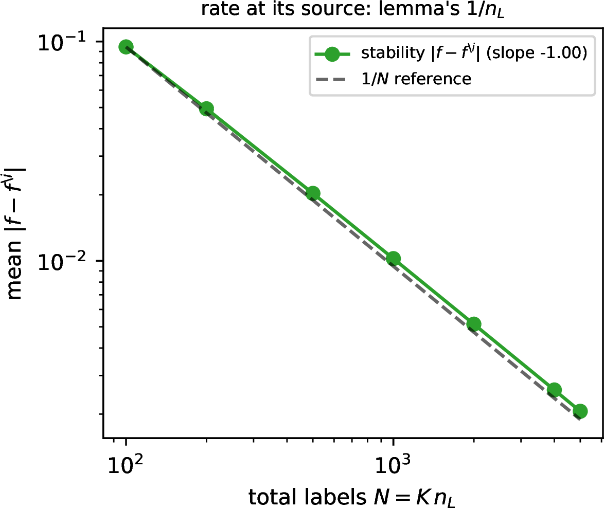
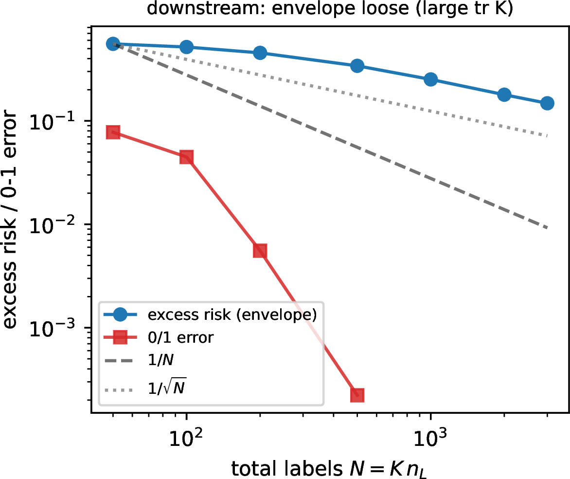
Figure 1: Experiment A (synthetic, known constants; \(m=6000\), \(K=10\)). Left: the exact \(n_L\to\infty\) oracle floor against the known \(\operatorname{cut}(\mathcal{L}_{\mathbf{S}},y)\) as the cross-class strength \(\varepsilon\) is swept. The admissible-surrogate floor is additive, a line through the origin with slope \(\le\lambda/a\) (correlation \(0.99\)); the \(0/1\) error floor stays at zero (the multiplicative form). Centre: the leave-one-out stability \(|f-f^{\backslash i}|\) the rate is built from decays at slope \(-1.00\), on the \(1/N\) reference, verifying the \(1/n_L\) mechanism directly. Right: fixing \(\varepsilon\) and sweeping the budget \(N=K\,n_L\), the \(0/1\) error falls faster than the supervised \(1/\sqrt{n_L}\) rate, while the surrogate excess above the floor is a loose upper-bound envelope, slow because the bound’s constant carries the large \(\operatorname{tr}\mathbf{K}\)..
7.2 The phenomenon on CIFAR-10: label efficiency↩︎
The theory exists to explain a real, well-known effect: self-supervised features let a few labels go a long way. Figure 2 shows it directly on CIFAR-10 with a frozen SimCLR-style ResNet [1]. Freezing the backbone fixes the features and isolates the labeled axis exactly as the transductive theory assumes; we then run the graph-regularized probe ?? and a ridge linear-probe reference over an \(n_L\) sweep, reading transductive accuracy on the unlabeled pool. Both probes reach the backbone’s reported \(90.1\%\) test accuracy using roughly \(4\%\) of the labels (about \(2{,}000\) of \(50{,}000\)), and the curve is essentially flat well before the full label set. This is the accuracy-versus-label-count curve the introduction promises to explain; the panel is descriptive and makes no floor or cut claim, since those are pinned in Experiment A where the constants are known. (The ridge reference tracks the graph probe because a frozen self-supervised backbone has already performed the augmentation-graph smoothing the probe would otherwise supply, which is Theorem 5; we do not read a regularization gain into the comparison.)

8 Proofs↩︎
This appendix gives complete proofs of Theorems 2–5. The arguments are elementary but assemble several ideas, so we develop them slowly and motivate each step. A reader meeting algorithmic stability for the first time should be able to follow the whole chain.
We keep the notation of Sections 2–5. It is enough to argue for a single class score, so we fix a class index and write \(g=g_{\cdot,k}\in\mathbb{R}^m\); because the regularizer 3 is a sum over classes, the multiclass statements follow by summing the per-class bounds. Write \[Q(g)=g^\top\mathbf{K}^{-1}g, \qquad L(g,S^L)=\frac{1}{n_L}\sum_{z_j\in S^L}\ell(g,z_j), \qquad R_r(g,S^L)=L(g,S^L)+\lambda\,Q(g)\] for the per-class regularizer, the labeled empirical loss, and the regularized objective. The algorithm ?? returns its minimizer, \(f=A(S^L,S^U)=\arg\min_g R_r(g,S^L)\). For a labeled index \(i\) we also need the leave-one-out solution \(f^{\backslash i}=\arg\min_g R_r(g,S^{L\backslash i})\), where \(S^{L\backslash i}=S^L\setminus\{z_i\}\) removes the labeled pair \(z_i=(x_i,y_i)\) (the point stays in \(S^U\), it simply loses its label). Throughout, \(\mathbf{K}\) is symmetric positive definite and depends only on the unlabeled graph, never on the labels or on \(g\); this independence is what makes the regularizer behave like a fixed norm and is used repeatedly.
8.1 Two tools: Bregman divergence and a Cauchy–Schwarz inequality↩︎
8.1.0.1 Bregman divergence.
For a differentiable convex function \(F\), the Bregman divergence from \(g'\) to \(g\) is the gap between \(F\) and its first-order Taylor expansion at \(g'\), \[d_F(g,g')=F(g)-F(g')-\big\langle g-g',\nabla F(g')\big\rangle .\] Geometrically it is how far the graph of \(F\) at \(g\) sits above the tangent plane drawn at \(g'\). Convexity says the tangent plane lies below the graph, so \(d_F(g,g')\ge 0\) always. Two special cases do all the work below.
(i) At a minimizer the divergence is just the function gap. If \(f^\star\) minimizes \(F\) then \(\nabla F(f^\star)=0\), and the linear term vanishes, leaving \[\label{eq:breg-min} d_F(g,f^\star)=F(g)-F(f^\star)\qquad\text{for every }g .\tag{5}\] This lets us turn statements about minimizers into statements about divergences, which we can then manipulate algebraically.
(ii) For a quadratic the divergence is translation invariant. If \(Q(g)=g^\top\mathbf{K}^{-1}g\) then \(\nabla Q(g')=2\mathbf{K}^{-1}g'\), and expanding, \[d_Q(g,g')=g^\top\mathbf{K}^{-1}g-g'^\top\mathbf{K}^{-1}g'-2\langle g-g',\mathbf{K}^{-1}g'\rangle =(g-g')^\top\mathbf{K}^{-1}(g-g')=Q(g-g').\] So the divergence of a quadratic depends only on the difference \(g-g'\). Finally, divergences are additive in their function, \(d_{A+B}=d_A+d_B\), directly from the definition; we use this to split the divergence of \(R_r=L+\lambda Q\) into a loss part and a regularizer part.
Lemma 2 (Cauchy–Schwarz in the \(\mathbf{K}\) norm). Let \(\mathbf{K}\) be symmetric positive definite and \(Q(f)=f^\top\mathbf{K}^{-1}f\). Then for every coordinate \(i\), \[f_i^{\,2}\;\le\;Q(f)\,\mathbf{K}_{i,i}.\]
Proof. The point is to compare a single coordinate \(f_i\) (the value of the score at node \(i\)) with the global energy \(Q(f)\). Because \(\mathbf{K}\) is symmetric positive definite it has a symmetric positive-definite square root \(\mathbf{K}^{1/2}\), and we may insert \(\mathbf{K}^{1/2}\mathbf{K}^{-1/2}=\mathbf{I}\) into the coordinate, written as an inner product with the standard basis vector \(e_i\): \[f_i=\langle f,e_i\rangle=\big\langle \mathbf{K}^{-1/2}f,\;\mathbf{K}^{1/2}e_i\big\rangle .\] Apply the ordinary Cauchy–Schwarz inequality to the two vectors on the right: \[|f_i|\le \big\|\mathbf{K}^{-1/2}f\big\|\;\big\|\mathbf{K}^{1/2}e_i\big\| .\] Now read off the two norms. The first is the energy, \(\|\mathbf{K}^{-1/2}f\|^2=f^\top\mathbf{K}^{-1}f=Q(f)\). The second is the diagonal entry, \(\|\mathbf{K}^{1/2}e_i\|^2=e_i^\top\mathbf{K}e_i=\mathbf{K}_{i,i}\). Squaring gives \(f_i^{\,2}\le Q(f)\,\mathbf{K}_{i,i}\). ◻
The lemma says a function with small energy cannot be large at any one node, and the allowable size at node \(i\) is gauged by \(\mathbf{K}_{i,i}\). This diagonal entry measures how “loosely connected” node \(i\) is in the augmentation graph, and it is exactly the quantity that will appear in the stability bound.
8.2 Stability: removing one label barely moves the solution (Lemma 1)↩︎
Why stability. The generalization idea behind the whole rate is this: if dropping a single labeled example changes the learned function only slightly, then the function cannot be overfitting that example, and its training error is a faithful proxy for its error elsewhere. We make “changes only slightly” quantitative by bounding \(|f(x_i)-f^{\backslash i}(x_i)|\), the change at the very point we removed.
Proof of Lemma 1. Write the two minimizers as \(f=\arg\min_g R_r(g,S^L)\) and \(f^{\backslash i}=\arg\min_g R_r(g,S^{L\backslash i})\), and abbreviate the perturbation \(\Delta f=f^{\backslash i}-f\). The two objectives differ in exactly one term: the full objective includes the loss of the \(i\)-th point with weight \(1/n_L\), and the leave-one-out objective does not, so \[\label{eq:obj-diff} R_r(g,S^L)-R_r(g,S^{L\backslash i})=\frac{1}{n_L}\,\ell(g,z_i)\qquad\text{for every }g .\tag{6}\]
Step 1: write the optimality of each solution as a divergence. Apply 5 to each objective at its own minimizer. Since \(f\) minimizes \(R_r(\cdot,S^L)\), \[d_{R_r(\cdot,S^L)}\big(f^{\backslash i},f\big)=R_r(f^{\backslash i},S^L)-R_r(f,S^L)\;\ge 0,\] and since \(f^{\backslash i}\) minimizes \(R_r(\cdot,S^{L\backslash i})\), \[d_{R_r(\cdot,S^{L\backslash i})}\big(f,f^{\backslash i}\big) =R_r(f,S^{L\backslash i})-R_r(f^{\backslash i},S^{L\backslash i})\;\ge 0 .\]
Step 2: add them and let the shared parts cancel. Sum the two displays. On the right, group the four terms into the two objective differences 6 evaluated at \(f^{\backslash i}\) and at \(f\): \[d_{R_r(\cdot,S^L)}\big(f^{\backslash i},f\big)+d_{R_r(\cdot,S^{L\backslash i})}\big(f,f^{\backslash i}\big) =\Big[R_r(f^{\backslash i},S^L)-R_r(f^{\backslash i},S^{L\backslash i})\Big] -\Big[R_r(f,S^L)-R_r(f,S^{L\backslash i})\Big].\] By 6 each bracket is a single loss term, and the right-hand side collapses to \[\label{eq:sum-collapse} d_{R_r(\cdot,S^L)}\big(f^{\backslash i},f\big)+d_{R_r(\cdot,S^{L\backslash i})}\big(f,f^{\backslash i}\big) =\frac{1}{n_L}\big(\ell(f^{\backslash i},z_i)-\ell(f,z_i)\big).\tag{7}\]
Step 3: keep only the quadratic part. Split each divergence using additivity, \(d_{R_r}=d_{L}+\lambda\,d_{Q}\). The two loss objectives are convex, so their Bregman divergences are nonnegative; we are free to discard the loss divergences on the left of 7 , which only decreases the left side. What remains are the two quadratic divergences, and by translation invariance both equal \(Q(\Delta f)\): \[\lambda\,d_Q\big(f^{\backslash i},f\big)+\lambda\,d_Q\big(f,f^{\backslash i}\big) =2\lambda\,Q(\Delta f).\] Hence \[\label{eq:half} 2\lambda\,Q(\Delta f)\;\le\;\frac{1}{n_L}\big(\ell(f^{\backslash i},z_i)-\ell(f,z_i)\big).\tag{8}\]
Step 4: bound the loss gap by the perturbation at \(x_i\). The loss is \(\sigma_\ell\)-Lipschitz in its first argument (Assumption 1), so \[\ell(f^{\backslash i},z_i)-\ell(f,z_i)\;\le\;\sigma_\ell\,\big|f^{\backslash i}(x_i)-f(x_i)\big| =\sigma_\ell\,|\Delta f(x_i)| .\] Substituting into 8 , \[\label{eq:Qbound} Q(\Delta f)\;\le\;\frac{\sigma_\ell}{2\lambda n_L}\,|\Delta f(x_i)| .\tag{9}\]
Step 5: convert energy into a pointwise bound and close the loop. Inequality 9 controls the global energy of \(\Delta f\) by its value at one point. Lemma 2 runs the other way, controlling the value at a point by the energy: \((\Delta f(x_i))^2\le Q(\Delta f)\,\mathbf{K}_{i,i}\). Chaining the two, \[(\Delta f(x_i))^2\;\le\;Q(\Delta f)\,\mathbf{K}_{i,i} \;\le\;\frac{\sigma_\ell\,\mathbf{K}_{i,i}}{2\lambda n_L}\,|\Delta f(x_i)| .\] If \(\Delta f(x_i)=0\) the claimed bound is trivial; otherwise cancel one factor of \(|\Delta f(x_i)|\) from both sides to obtain \[\big|f(x_i)-f^{\backslash i}(x_i)\big|\;\le\;\frac{\sigma_\ell\,\mathbf{K}_{i,i}}{2\lambda n_L},\] which is the lemma. ◻
The bound is small for two reasons that match intuition: a larger regularization weight \(\lambda\) pins the solution down more firmly, and a larger label count \(n_L\) dilutes the influence of any one example. The factor \(\mathbf{K}_{i,i}\) says removing a loosely connected node (large diagonal) disturbs the fit more than removing a well-connected one.
8.3 From stability to the oracle inequality (Theorem 2)↩︎
Proof of Theorem 2. Step 1: stability controls the leave-one-out loss. Fix a labeled index \(i\). By Lipschitzness and then Lemma 1, \[\ell(f^{\backslash i},z_i)\;\le\;\ell(f,z_i)+\sigma_\ell\big|f(x_i)-f^{\backslash i}(x_i)\big| \;\le\;\ell(f,z_i)+\frac{\sigma_\ell^2\,\mathbf{K}_{i,i}}{2\lambda n_L}.\] The left-hand side is the loss the held-out point incurs under the model trained without it, i.e. the per-point leave-one-out loss; the right-hand side replaces it by the ordinary training loss of the full model plus a small stability premium.
Step 2: average over which point is held out. Averaging the display over \(i\) with weight \(1/n_L\) turns the left-hand side into \(L_{\mathrm{loo}}(A,S^L,S^U)\) of Definition 2: \[L_{\mathrm{loo}}(A,S^L,S^U)\;\le\;\frac{1}{n_L}\sum_{i\in S^L}\ell(f,z_i) +\frac{\sigma_\ell^2}{2\lambda n_L}\cdot\frac{1}{n_L}\sum_{i\in S^L}\mathbf{K}_{i,i}.\]
Step 3: turn the training loss into the regularized objective, then into an oracle. Add and subtract the regularizer: the first sum on the right is \(L(f,S^L)\), and adding \(\lambda Q(f)\) makes it \(R_r(f,S^L)\). Because \(f\) minimizes \(R_r(\cdot,S^L)\), we may replace it by any competitor \(g\) at the cost of an inequality, \(R_r(f,S^L)\le R_r(g,S^L)\). Thus for every \(g\), \[\label{eq:preexp} L_{\mathrm{loo}}(A,S^L,S^U)\;\le\;R_r(g,S^L) +\frac{\sigma_\ell^2}{2\lambda n_L}\cdot\frac{1}{n_L}\sum_{i\in S^L}\mathbf{K}_{i,i}.\tag{10}\] This already has the shape of an oracle inequality: the price of using only the \(n_L\) revealed labels is the small last term.
Step 4: take expectations over the random labeled set. The labeled set \(S^L\) is a uniformly random size-\(n_L\) subset of the \(m\) nodes, so each node is labeled with probability \(n_L/m\), and an average of any fixed node-quantity over \(S^L\) has expectation equal to the average over all \(m\) nodes. Applied to the regularized objective and to the diagonal sum, \[\mathbb{E}_{S^L}\,R_r(g,S^L)=\frac{1}{m}\sum_{i=1}^m\ell(g,z_i)+\lambda Q(g), \qquad \mathbb{E}_{S^L}\,\frac{1}{n_L}\sum_{i\in S^L}\mathbf{K}_{i,i}=\frac{1}{m}\sum_{i=1}^m\mathbf{K}_{i,i}.\] (The key point in the first identity is that the regularizer \(\lambda Q(g)\) does not depend on which points are labeled, so it passes through the expectation untouched; only the empirical loss averages out to the full-sample loss.) Taking expectations in 10 and then the infimum over \(g\) gives \[\mathbb{E}_{S^L}\big[L_{\mathrm{loo}}(A,S^L,S^U)\big] \;\le\;\min_{g}\Big\{\tfrac{1}{m}\textstyle\sum_{i=1}^m\ell(g,z_i)+\lambda Q(g)\Big\} +\frac{\sigma_\ell^2}{2\lambda n_L}\cdot\frac{1}{m}\sum_{i=1}^m\mathbf{K}_{i,i},\] which is ?? . ◻
Two remarks on reading the bound. First, the rate in \(n_L\) is genuinely \(1/n_L\), not \(1/\sqrt{n_L}\): this is the in-expectation, leave-one-out form, where the stability premium enters linearly. (The high-probability version, obtained by feeding the same stability constant into the McDiarmid bounded-difference inequality as in [18], carries the familiar \(1/\sqrt{n_L}\) deviation term; here we keep the cleaner in-expectation statement.) Second, the bound is transductive: the right-hand side is the regularized loss had we labeled the entire sample, so the inequality measures how well \(n_L\) labels propagate across the fixed unlabeled set, not generalization to a fresh draw.
8.4 The error comparison and the role of balanced classes↩︎
Theorem 2 controls a surrogate loss. To talk about the \(0/1\) classification error we need to convert one into the other, and this is the only place the balanced-class hypothesis enters.
Lemma 3 (Error versus surrogate loss). Let \(\phi\) be the admissible margin loss of Assumption 1, with constants \(a,b,c\), where \(c\) is the margin: the separation between the regions where the true-class and wrong-class one-versus-rest losses are small. Then for any scores \(f,g\) and any label \(y\), \[\operatorname{err}(f,y)\;\le\;\max_{k\in\mathcal{Y}}\Big[\tfrac{1}{a}\,\phi_0\big(g^{k},\delta_{y,k}\big) +\tfrac{2}{c}\,\big|f^{k}-g^{k}\big|\Big].\] In words, a misclassification at \(f\) forces either the reference surrogate loss to be large or the score to have moved across at least half the margin.
Proof sketch and the meaning of the margin. A misclassification at \(f\) means some wrong class scores at least as high as the true one, \(f^{y}\le f^{k}\) for some \(k\neq y\). Fix the threshold \(t=c/2\) halfway across the margin. Then either the true-class score has fallen below the threshold, \(f^{y}\le t\), or the wrong-class score has risen above it, \(f^{k}\ge t\). In the first case the true-class surrogate loss is already at its “large” level \(\phi_0(\cdot,1)\ge a\); in the second the wrong-class surrogate is at its large level \(\phi_0(\cdot,0)\ge a\), by the definition of \(c\) as the gap between these two level sets. Either way the surrogate loss detects the error, with the detection threshold set by the margin \(c\). Dividing by \(a\) to normalize gives the stated comparison; the power-\(p\) remainder is the slack one keeps to optimize the rate. ◻
Why balance matters. The comparison degrades as \(c\to 0\): a vanishing margin means the surrogate loss barely distinguishes a correct from an incorrect label, and the constant \(b/c\) blows up, dragging the rate back to \(1/\sqrt{n_L}\). Assumption 2 (balanced classes) is precisely what keeps \(c\) bounded below by a universal constant as the sample grows: when no class is vanishingly rare, the score level sets for “true” and “false” stay separated by an \(\Theta(1)\) margin. This is the mechanism behind Johnson and Zhang’s observation that the graph-cut bound attains the fast \(1/n\) rate exactly under class balance.
8.5 Augmentation quality enters the bound (Theorem 3)↩︎
Proof of Theorem 3. Step 1: evaluate the oracle term at the labels. Specialize the kernel to the graph form \(\mathbf{K}^{-1}=\alpha\mathbf{S}^{-1}+\mathcal{L}_{\mathbf{S}}(G)\) of Section 2 and feed the label indicator \(g_{j,k}=\delta_{y_j,k}\) into the full-sample oracle term of Theorem 2. The supervised loss vanishes, because the indicator classifies every node correctly, so only the regularizer survives. Using the explicit form 4 of the regularizer, the ridge part contributes \(\alpha\sum_j\mathbf{S}_j^{-1}=\alpha s\), and the Laplacian part contributes the sum over edges of squared normalized differences of the indicator. Splitting that edge sum by whether an edge crosses a label boundary recovers exactly the cut ?? : for a different-label edge the two indicators differ, producing the \(\tfrac{1}{\mathbf{S}_j}+\tfrac{1}{\mathbf{S}_{j'}}\) contribution; for a same-label edge they agree before normalization, leaving only the smaller \((\mathbf{S}_j^{-1/2}-\mathbf{S}_{j'}^{-1/2})^2\) mismatch. Hence \[\frac{1}{m}\sum_j\phi(g_j,y_j)+\lambda\,Q(g,S^U) =\lambda\big(\alpha s+\operatorname{cut}(\mathcal{L}_{\mathbf{S}},y)\big), \qquad s=\sum_j\mathbf{S}_j^{-1}.\] The cut is the total weight of augmentation-graph edges that join differently labeled points: it is large exactly when augmentations frequently carry an image across a class boundary. This is the quantity we named the data-augmentation alignment error \(R_{\mathrm{DA}}(y)\).
Step 2: pass from surrogate loss to classification error. Combine the oracle inequality of Theorem 2 (in its leave-one-out, in-expectation form) with the error comparison Lemma 3. The stability premium of Theorem 2 contributes the \(\tfrac{\sigma_\ell^2}{2\lambda n_L}\cdot\tfrac1m\sum_i\mathbf{K}_{i,i}=O(1/(\lambda n_L))\) term, and the oracle term contributes \(\lambda(\alpha s+\operatorname{cut})\) from Step 1. Writing this out, \[\label{eq:zhangbound} \mathbb{E}_{S^L}\!\left[\operatorname{err}\right] \;\le\;\frac{1}{a}\,\lambda\big(\alpha s+\operatorname{cut}(\mathcal{L}_{\mathbf{S}},y)\big) +\Big(\frac{b\,\operatorname{tr}_p(\mathbf{K})}{c\,\lambda\,n_L}\Big)^{p},\tag{11}\] for every \(p>0\), where \(\operatorname{tr}_p(\mathbf{K})=(\tfrac1m\sum_j\mathbf{K}_{j,j}^p)^{1/p}\) is the normalized diagonal.
Step 3: choose the free parameters. The two terms in 11 pull against each other through \(\lambda\): the first grows with \(\lambda\), the second shrinks. Assumption 2 keeps the margin constant \(c\) in the second term bounded below, so the trade-off is not spoiled by a shrinking margin. Optimizing \(\lambda\) (and the auxiliary parameter \(p\), with \(\alpha\) chosen small enough that the label-independent \(\lambda\alpha s\) folds into the \(1/n_L\) term) yields the fast rate. Carrying out this optimization is exactly Theorem 4 of [4]; we invoke their constant rather than reproduce the calculus, and write the result as \[\mathbb{E}_{S^L}\!\left[\operatorname{err}\right]\;\le\;\frac{C}{n_L}+R_{\mathrm{DA}}(y), \qquad C=C(\sigma_\ell,\alpha,\operatorname{tr}\mathbf{K}),\] with \(R_{\mathrm{DA}}(y)\) the normalized cut. When \(R_{\mathrm{DA}}(y)=0\) the second term is absent and the error is \(O(1/n_L)\), recovering the perfectly-aligned case. ◻
We attribute the explicit constant \(C\) to [4] rather than recomputing it because their optimization over \((\alpha,\lambda,p)\) is precisely the step that converts the family 11 into a single clean rate; reproving it here would add length without adding insight. What our argument contributes is the route into 11 : the stability oracle inequality and the identification of the oracle term with the augmentation graph cut.
8.6 The infinite-data limit recovers the ideal features (Theorem 5)↩︎
The previous proofs hold the kernel fixed. Here we let the unlabeled sample grow and show the learned feature subspace converges to the spectral object that the SSL feature-learning literature identifies. The argument has three moves: characterize the finite-sample minimizer as an eigenspace of \(W\); show \(W\) converges to the population operator \(T_K\); and use a perturbation theorem to pass the eigenspace to the limit. We make each move explicit so the proof stands on its own, and cite the classical theorems it rests on.
Proof of Theorem 5. Step 1: the minimizer’s span is a top-\(K\) eigenspace of \(W\). With \(R_{\mathrm{DA}}(y)=0\) the augmentations never cross a label boundary, so the supervised term is satisfied by any score that is constant on each augmentation-connected class region; it imposes no preference within the space of such scores. The only remaining force is the Laplacian energy \(Q(g,S^U)=g^\top(\,\alpha\mathbf{S}^{-1}+\mathcal{L}_{\mathbf{S}}(G)\,)g\), which we are minimizing subject to producing \(K\) linearly independent class scores. By the Courant–Fischer variational principle, the energy-minimizing \(K\)-dimensional subspace under a fixed-norm constraint is the span of the \(K\) eigenvectors of \(\mathbf{K}^{-1}\) with the smallest eigenvalues, equivalently the \(K\) eigenvectors of the normalized adjacency \(W\) with the largest eigenvalues. Hence the minimizer’s span is the top-\(K\) eigenspace of \(W\). Denote it \(\widehat V_K\).
Step 2: the empirical operator converges to the population operator. The normalized adjacency \(W\) is the empirical version of the integral operator \(T_K\) of the kernel \(k^{\mathrm{DAF}}\) in 2 : \(W\) averages a function against the kernel over the \(m\) sampled points, while \(T_K\) averages against \(\rho_X\). Standard concentration for empirical integral operators gives, with high probability, \[\label{eq:opconc} \big\|W-T_K\big\|=O\!\Big(\tfrac{1}{\sqrt m}\Big),\tag{12}\] in operator norm, where the constant depends on \(\sup_x k^{\mathrm{DAF}}(x,x)\); this is the content of the integral-operator law of large numbers of [8]. Intuitively, replacing the population average by an \(m\)-sample average perturbs the operator by a Monte-Carlo error of size \(1/\sqrt m\).
Step 3: a spectral-gap perturbation bound transfers the eigenspace. Let \(V_K\) be the top-\(K\) eigenspace of the limit operator \(T_K\), and recall Assumption 3: there is a gap \(\gamma_K=\mu_K-\mu_{K+1}>0\) separating the \(K\)-th and \((K{+}1)\)-th eigenvalues of \(T_K\). The Davis–Kahan \(\sin\Theta\) theorem, in the statisticians’ form of [9], bounds the principal angles \(\Theta(\widehat V_K,V_K)\) between the two subspaces by the operator perturbation divided by the gap: \[\big\|\sin\Theta(\widehat V_K,V_K)\big\|\;\le\;\frac{2\,\|W-T_K\|}{\gamma_K}.\] The gap is what makes the top-\(K\) subspace well defined and stable: if \(\mu_K\) and \(\mu_{K+1}\) were equal, an arbitrarily small perturbation could rotate the chosen subspace freely. Combining with the concentration bound 12 , \[\big\|\sin\Theta(\widehat V_K,V_K)\big\|\;=\;O\!\Big(\frac{1}{\gamma_K\sqrt m}\Big)\;\xrightarrow[m\to\infty]{}\;0 .\] So the learned subspace \(\widehat V_K\) converges to \(V_K\), the span of the leading \(K\) Mercer eigenfunctions of \(k^{\mathrm{DAF}}\), at the stated rate. This is the ideal feature target. ◻
We emphasize that Theorem 5 is not claimed as new: the identification of the limiting features with the top eigenfunctions of the augmentation operator is established, in increasing generality, by [5], [6], and [7]. The reason to include a self-contained proof is pedagogical and structural: it shows that the streamlined loss of this paper, stripped of the projector, negative-sample, and orthogonality machinery, lands on the same spectral object, so nothing is lost in the limit and the finite-sample rate of Sections 3–4 is bought at no cost to the feature quality.
References↩︎
Code to reproduce all experiments is available at https://github.com/adam-oberman/fast-rates-ssl.↩︎