Forced condensation and anti-condensation on heavy-tailed networks
January 01, 1970
Abstract
We study a driven selection mechanism on a fixed heavy-tailed network. At each step fresh mass is injected, its direction is recomputed from the current mass profile by a power-normalization rule, and the combined mass is transported by a primitive mixing matrix. The exponent \(\theta\) controls the feedback. Positive values give more weight to larger coordinates, while negative values favor smaller ones. When \(\theta=0\), the injected mass is distributed uniformly. After deterministic growth of the total mass is scaled out, the long-run injection profile is characterized by a nonlinear Perron–Frobenius fixed point on the simplex. Hilbert’s projective metric gives a simple way to understand the stability of the system. The discounted network response brings positive profiles closer together, while the escort map scales their projective distance by \(|\theta|\). On heavy-tailed networks this fixed point separates three effects that are often conflated: response or degree tilt, anomalous inverse-participation-ratio scaling, and genuine few-node localization. Positive feedback selects high-response nodes and, when response follows degree, a hub-directed branch. Negative feedback selects low-response nodes and typically produces a broad peripheral cloud unless the lower tail of the response field is itself thin. Numerical experiments on finite power-law networks support these results. They show convergence, illustrate when the forcing rate becomes unimportant because mixing is sufficiently fast, and confirm both the sign law and the crossover in the participation ratio. This mechanism is different from both conserved-mass condensation and graph growth. Instead, feedback selects a non-equilibrium profile on a fixed, heterogeneous network.
non-equilibrium statistical mechanics ,complex networks ,condensation ,heavy-tailed networks ,nonlinear Perron–Frobenius theory ,Hilbert metric
1 Introduction↩︎
Condensation is one of the simplest ways in which a many-component system can become very unequal. In a zero-range or mass-transport process, a large share of the conserved mass can collect at a single site. In a growing network, a node with a fitness advantage can acquire a finite fraction of all links. Similar concentration can arise in multiplicative economic models, where wealth may become concentrated among a small number of agents [1]. These examples differ in their details, but they share a common warning: in a heterogeneous system, the interesting object is often not the total amount of mass, but the normalized profile selected by the dynamics.
This paper studies a deliberately spare version of that question. The network is fixed. It is not grown by preferential attachment during the dynamics. The total mass is not conserved either. Fresh mass is injected at every step, the injection direction is chosen from the current mass profile, and the network then mixes the result. The feedback rule is a power law. If \(\theta>0\), nodes that already carry more mass receive a larger share of the next injection. If \(\theta<0\), the rule is reversed and the next injection favors smaller coordinates. The case \(\theta=0\) is the neutral baseline.
The model was chosen to isolate a specific mechanism. Condensation in complex networks is usually discussed through conserved stochastic transport, zero-range processes, balls-in-boxes models, eigenvector localization, or graph growth with preferential attachment and fitness [2]–[8]. Those mechanisms are important, but they mix several ingredients. Here the substrate is fixed and the total mass grows in a trivial deterministic way. All non-trivial behavior lies in the shape of the profile after this growth is divided out. This makes it possible to ask a clean statistical-mechanics question: what profile is selected by feedback on a fixed heterogeneous network, and how does the answer depend on the sign and strength of the feedback?
The answer comes in two parts. The first is that the normalized dynamics has a fixed point, and we give explicit mixing–forcing conditions under which the original recursion converges to it. The fixed point is a nonlinear Perron–Frobenius object [9]. The linear part is a discounted resolvent of the network matrix, and the nonlinear part is the escort, or power-normalization, map. Hilbert’s projective metric gives the useful estimate: the positive network resolvent contracts projective distances, while the escort map multiplies them exactly by \(|\theta|\). The frozen-response map is therefore contractive throughout the concave range \(|\theta|<1\), with a somewhat larger fixed-point window when the network response is strongly mixing.
The second is that on a heavy-tailed network this fixed point is not described by a single word such as “condensed”. There is a degree tilt, a participation-ratio transition, and a stronger few-node localization limit. They need not occur at the same place. Positive feedback tilts mass toward high-degree or high-centrality nodes; negative feedback tilts it toward the periphery. Yet the inverse participation ratio may remain of order \(1/n\) throughout a broad range, even while the degree tilt is visible. Anti-condensation, in particular, is usually broad: if linearly many nodes sit at the lower end of the network response, negative feedback spreads mass across that peripheral class rather than placing it on one or two nodes.
The contrast with the standard pictures is instructive. In a zero-range process the total mass is fixed and the condensate is produced by stochastic transport. In a growing-network model the substrate itself changes and the winner may be a node that captures links. Here neither mechanism is present. The substrate is fixed, total growth is deterministic, and the only question is the shape of the non-equilibrium profile selected by feedback. The transition is therefore closer to a driven steady-state selection problem than to an equilibrium condensation of a conserved field.
The point can be put more concretely. If the forcing were fixed in advance, the long-run profile would be the ordinary linear response of the network. If the network response were completely homogeneous, the escort rule would have no structural information on which to act. The effect studied here appears only when both ingredients are present: the graph creates a heterogeneous response field, and the feedback rule repeatedly reweights the next injection against that field. That is what makes the sign of \(\theta\) decisive. Positive feedback rewards large response coordinates, whereas negative feedback uses the same response field in the opposite direction.
The word “condensation” will therefore be used with some care. A hub-biased profile is not automatically a condensate. A profile may have a large covariance with degree while still spreading its mass over a linear number of nodes. Conversely, a high inverse participation ratio is a stricter statement about effective support. The paper keeps these diagnostics separate because a heavy-tailed graph can make them disagree over a wide parameter range, and nowhere more so than on the negative branch, where the selected low-response set can contain many nodes.
Once the selected injection profile is known, one may also study the corresponding standing stock and the currents induced by transport. Those quantities can be useful on directed networks, but they are not needed for the condensation argument developed here; their definitions and basic identities are collected in the Supplementary Material (Sec. S5), and they are not pursued further in this paper.
The paper is organized as follows. Section 2 defines the forced mixing process and derives the autonomous limiting map. Section 3 gives a fixed-point result and an explicit sufficient condition for convergence of the original recursion. Section 4 gives the reverse-kernel and linear-response interpretation of the fixed point. Section 5 gives the heavy-tail analysis: a two-block sign law, its degree-class extension, and the participation-ratio transition. Section 6 presents finite-network simulations.
2 Model and limiting map↩︎
Vectors are columns. The network matrix acts on the left, and a column-stochastic matrix preserves total mass. Fix \(n\in\mathbb{N}\) and write \[S_{n-1}=\{x\in\mathbb{R}_{\ge0}^n:\mathbf{1}^\top x=1\},\qquad S_{n-1}^\circ=S_{n-1}\cap\mathbb{R}_{>0}^n .\] The network is represented by a matrix \(\mathbf{A}\in\mathbb{R}_{\ge0}^{n\times n}\).
Assumption 1. The matrix \(\mathbf{A}\) is column-stochastic and primitive: \[\mathbf{1}^\top\mathbf{A}=\mathbf{1}^\top,\qquad \mathbf{A}^k>0\;entrywise for some k\ge1 .\]
Column-stochasticity says that the mixing step neither creates nor destroys mass. Primitivity is the finite-state irreducibility-and-aperiodicity assumption: a perturbation can eventually be felt everywhere.
Let \(\pi>0\) be the forcing rate and \(\theta\in\mathbb{R}\) the feedback exponent. For \(u\in\mathbb{R}_{>0}^n\) define the escort map [10] \[\label{eq:Ptheta95def} P_\theta(u)=\frac{u^{\circ\theta}}{\mathbf{1}^\top u^{\circ\theta}},\qquad P_0(u)=\frac{1}{n}\mathbf{1} .\tag{1}\] The power is componentwise. For \(\theta>0\), the same formula is used on \(\mathbb{R}_{\ge0}^n\setminus\{0\}\) with the convention \(0^\theta=0\); for \(\theta<0\), all coordinates must be positive. We take \(m_0\in\mathbb{R}_{\ge0}^n\setminus\{0\}\), with \(m_0\in\mathbb{R}_{>0}^n\) when \(\theta<0\). The mass vector then evolves by \[\label{eq:m95recursion} m_{t+1}=\mathbf{A}\bigl(m_t+\pi M_t\,\gamma_t\bigr),\qquad M_t=\mathbf{1}^\top m_t,\qquad \gamma_t=P_\theta(m_t).\tag{2}\] Since \(\mathbf{1}^\top\gamma_t=1\) and \(\mathbf{A}\) is column-stochastic, \[M_{t+1}=(1+\pi)M_t,\qquad M_t=(1+\pi)^tM_0 .\] Thus the total mass grows at a fixed deterministic rate. The non-trivial object is the profile \(\gamma_t\).
Set \[a=\frac{1}{1+\pi},\qquad b=\frac{\pi}{1+\pi},\qquad u_t=a^t m_t .\] By homogeneity of \(P_\theta\), \(\gamma_t=P_\theta(u_t)\), and the rescaled recursion is \[\label{eq:u95recursion} u_{t+1}=a\mathbf{A} u_t+bM_0\,\mathbf{A}\gamma_t,\qquad \gamma_{t+1}=P_\theta(u_{t+1}).\tag{3}\] If the forcing profile were frozen at \(z\in S_{n-1}\), the stable linear filter in 3 would converge to \[w(z)=bM_0\,\mathbf{A}(I-a\mathbf{A})^{-1}z .\] This motivates the positive response matrix \[\label{eq:Lpi95def} \mathbf{L}_\pi =bM_0\,\mathbf{A}(I-a\mathbf{A})^{-1} =bM_0\sum_{k=0}^{\infty}a^k\mathbf{A}^{k+1}.\tag{4}\] The series form is useful: a unit of injected mass is mixed once, then mixed again and again, with discount \(a^k\). The corresponding autonomous map on the simplex is \[\label{eq:T95def} T(z)=P_\theta(\mathbf{L}_\pi z).\tag{5}\] The following normalization will be used repeatedly. Because \(\mathbf{1}^\top\mathbf{L}_\pi=M_0\mathbf{1}^\top\), the matrix \[\label{eq:Q95def} \mathbf{Q}=\frac{1}{M_0}\mathbf{L}_\pi\tag{6}\] is strictly positive and column-stochastic. Since \(P_\theta\) is homogeneous, \(T(z)=P_\theta(\mathbf{Q}z)\).
The role of the forcing rate \(\pi\) is easy to misread, so we pin it down before moving on. It changes the memory length in the resolvent. Large \(\pi\) makes \(a\) small, so recent injections dominate; small \(\pi\) makes \(a\) close to one, so older transported mass still matters. A “\(\pi\)-free” approximation is therefore not universal. It is accurate only when mixing over the resolvent horizon is rapid. For a well-conditioned network with a spectral gap, the relevant ratio is \(\pi/(1-|\lambda_2|)\); more generally it is the forcing time scale relative to the mixing time. In that regime the response approaches the Perron profile and the normalized fixed point depends mainly on the response field and on \(\theta\). This restricted statement is what is tested in the simulations.
The matrix \(\mathbf{Q}\) also has a useful probabilistic reading. It is the average destination of a unit of mass after one mandatory network step and then a geometrically distributed number of further steps. Thus the escort rule decides where mass is injected, while \(\mathbf{Q}\) describes the response seen after transport. The fixed point says that these two descriptions are consistent after the power normalization.
Two modeling choices deserve a word. The use of a column-stochastic network matrix is only a normalization of the transport step: it says that the transport operator redistributes existing mass before the next injection arrives. Other physical normalizations can be reduced to this one after rescaling by the natural conserved left eigenvector, provided the resulting positive cone is preserved. Primitivity, in turn, is not meant to exclude sparse networks. It is a finite-state regularity assumption ensuring that the discounted response is strictly positive. In simulations one can work with sparse primitive matrices; the resolvent is then applied through matrix-vector products or truncated filters rather than stored as a dense matrix.
The parameter \(\pi\) should also be read physically. The mean number of extra network steps in the resolvent is \((1-\!a)^{-1}-1=1/\pi\). Thus small \(\pi\) lets injected mass travel for many steps before being effectively discounted, while large \(\pi\) emphasizes the first few transport steps after injection. This affects the quantitative response field, but not the basic sign mechanism. Once \(\mathbf{Q}\) is known, the fixed point is controlled by the competition between the projective contraction of \(\mathbf{Q}\) and the amplification \(|\theta|\) of the escort map.
3 Fixed point and convergence↩︎
The proof uses Hilbert’s projective metric. For \(x,y\in\mathbb{R}_{>0}^n\) set \[\label{eq:Hilbert95def} d_H(x,y)=\log\frac{\max_i x_i/y_i}{\min_i x_i/y_i}.\tag{7}\] It ignores scale and therefore fits the normalized problem. Since \(\mathbf{L}_\pi\) is strictly positive, its projective diameter \[\Delta_\pi=\log\max_{i,j,k,\ell} \frac{(\mathbf{L}_\pi)_{ik}(\mathbf{L}_\pi)_{j\ell}}{(\mathbf{L}_\pi)_{i\ell}(\mathbf{L}_\pi)_{jk}}\] is finite. Birkhoff’s theorem [11], [12] gives the contraction factor \[\tilde{q}=\tanh(\Delta_\pi/4)\in(0,1)\] (or any larger valid Birkhoff factor). The escort map scales projective distance exactly: \[\label{eq:escort95scaling} d_H(P_\theta(u),P_\theta(v))=|\theta|\,d_H(u,v).\tag{8}\] The identity is immediate: the componentwise power sends each ratio \(u_i/v_i\) to \((u_i/v_i)^\theta\), the normalization cancels from \(d_H\), and for \(\theta<0\) the maximal and minimal ratios exchange roles, which is where the modulus comes from. Consequently, \[\label{eq:T95contraction} d_H(Tx,Ty)\le |\theta|\tilde{q}\,d_H(x,y),\qquad x,y\in S_{n-1}^\circ .\tag{9}\] Because \(\mathbf{L}_\pi>0\), the map \(T\) extends continuously to the compact simplex \(S_{n-1}\) and maps it into \(S_{n-1}^\circ\). Brouwer’s theorem therefore gives at least one fixed point for every \(\theta\). When \(q:=|\theta|\tilde{q}<1\), the frozen-response map is a strict contraction and its fixed point is unique; in particular, uniqueness holds throughout \(|\theta|<1\). This statement concerns \(T\) itself; convergence of the original finite-memory recursion requires one additional, explicit small-gain condition.
The distinction is worth spelling out. The actual recursion 3 is not the Picard iteration of \(T\): at time \(t\), the state \(u_t\) retains the response to earlier injection profiles, whereas \(T\) uses the response that would result if the present profile were frozen indefinitely. The filter is stable because \(a<1\), but its tracking error must still be controlled.
For a fully explicit sufficient condition, choose \(k_0\ge1\) with \(\mathbf{A}^{k_0}>0\) and set \[\underline u=bM_0a^{k_0-1} \min_{i,j}(\mathbf{A}^{k_0})_{ij}, \qquad \ell_\pi=\min_{i,j}(\mathbf{L}_\pi)_{ij}, \qquad m_U=\min\{\underline u,\ell_\pi\}.\] After \(k_0\) steps, both the rescaled state and its frozen response have every coordinate at least \(m_U\) and total mass \(M_0\). Define \[C_U=\frac{2}{m_U}, \qquad D_W=2\log\frac{M_0}{\ell_\pi}, \qquad C_W=M_0\frac{e^{D_W}-1}{D_W},\] where \(C_W=M_0\) when \(D_W=0\). These constants are deliberately conservative. They enter through two elementary comparisons between Hilbert’s metric and the \(\ell^1\) norm, recorded once here because both directions are used below.
Lemma 1 (Metric comparison). Let \(x,y\in\mathbb{R}_{>0}^n\). (i) If \(x\ge m\mathbf{1}\) and \(y\ge m\mathbf{1}\) for some \(m>0\), then \[d_H(x,y)\le\frac{2}{m}\,\|x-y\|_1 .\] (ii) If \(\mathbf{1}^\top x=\mathbf{1}^\top y=M_0\) and \(x,y\ge\ell\,\mathbf{1}\) for some \(\ell>0\), then \(d_H(x,y)\le D\) with \(D=2\log(M_0/\ell)\), and \[\|x-y\|_1\le M_0\,\frac{e^{D}-1}{D}\,d_H(x,y).\]
Proof. (i) For each \(i\), \(|\log(x_i/y_i)|\le|x_i-y_i|/\min(x_i,y_i)\le\|x-y\|_1/m\), and \(d_H(x,y)\le2\max_i|\log(x_i/y_i)|\).
(ii) Every coordinate of \(x\) is at most \(M_0\) and every coordinate of \(y\) is at least \(\ell\), so each ratio \(r_i=x_i/y_i\) lies in \([\ell/M_0,M_0/\ell]\) and \(d_H(x,y)\le D\). Equality of the total masses forces \(\min_i r_i\le1\le\max_i r_i\), hence \(r_i\in[e^{-d},e^{d}]\) with \(d=d_H(x,y)\), and \(|r_i-1|\le e^{d}-1\le[(e^{D}-1)/D]\,d\) because \(t\mapsto(e^t-1)/t\) is increasing on \((0,\infty)\). Multiplying by \(y_i\) and summing over \(i\) gives the claim. ◻
Part (i) will be applied with \(m=m_U\) and part (ii) with \(\ell=\ell_\pi\); these choices produce the constants \(C_U\) and \(C_W\). With \(q=|\theta|\tilde{q}\), put \[\label{eq:small95gain95matrix} \mathsf M= \begin{pmatrix} q & |\theta|C_Ua\\[2pt] C_W\tilde{q}(1+q) & a\bigl(1+|\theta|C_UC_W\tilde{q}\bigr) \end{pmatrix}.\tag{10}\]
Proof. Write \(w^t=\mathbf{L}_\pi\gamma_t\), \(\delta_t=\|u_t-w^t\|_1\), and \(e_t=d_H(\gamma_t,\gamma_\star)\). Unrolling 3 over \(k_0\) steps gives \[u_{t+k_0}=a^{k_0}\mathbf{A}^{k_0}u_t+bM_0\sum_{s=0}^{k_0-1}a^s\mathbf{A}^{s+1}\gamma_{t+k_0-1-s},\] and the oldest injection term alone is \(bM_0a^{k_0-1}\mathbf{A}^{k_0}\gamma_t\ge\underline u\,\mathbf{1}\), because \(\mathbf{A}^{k_0}z\ge\min_{i,j}(\mathbf{A}^{k_0})_{ij}\,\mathbf{1}\) for every \(z\in S_{n-1}\). Hence \(u_t\ge\underline u\,\mathbf{1}\) for \(t\ge k_0\); also \(w^t\ge\ell_\pi\,\mathbf{1}\) for every \(t\). Both vectors have total mass \(M_0\) (the recursion preserves \(\mathbf{1}^\top u_t=M_0\) because \(a+b=1\)), so after burn-in they lie in the same compact positive coordinate box.
Because \(w^t\) is the fixed point of the frozen filter, \(w^t=a\mathbf{A}w^t+bM_0\mathbf{A}\gamma_t\); subtracting this from 3 gives \(u_{t+1}-w^t=a\mathbf{A}(u_t-w^t)\), and \(\|\mathbf{A}\|_{1\to1}=1\) then gives \[\label{eq:delta95first95bound} \delta_{t+1}\le a\delta_t+\|w^{t+1}-w^t\|_1.\tag{11}\] The vectors \(w^{t+1}\) and \(w^t\) have mass \(M_0\) and coordinates at least \(\ell_\pi\), so Lemma 1(ii), applied with \(\ell=\ell_\pi\) and combined with the Birkhoff contraction of \(\mathbf{L}_\pi\), yields \[\label{eq:w95motion95bound} \|w^{t+1}-w^t\|_1\le C_W\tilde{q}\,d_H(\gamma_{t+1},\gamma_t).\tag{12}\] Next, \(\gamma_{t+1}=P_\theta(u_{t+1})\) and \(T(\gamma_t)=P_\theta(w^t)\), so the exact scaling 8 gives \(\varepsilon_t:=d_H\bigl(\gamma_{t+1},T(\gamma_t)\bigr)=|\theta|\,d_H(u_{t+1},w^t)\). For \(t\ge k_0\) both arguments have coordinates at least \(m_U\), while \(\|u_{t+1}-w^t\|_1\le a\delta_t\), so Lemma 1(i) gives \[\varepsilon_t\le |\theta|C_Ua\,\delta_t,\] and the contraction of \(T\) gives \[\label{eq:e95tracking95bound} e_{t+1}\le q e_t+|\theta|C_Ua\,\delta_t.\tag{13}\] Finally, the triangle inequality gives \[d_H(\gamma_{t+1},\gamma_t) \le\varepsilon_t+(1+q)e_t.\] Combining this with 11 –13 gives, for \(t\ge k_0\), \[\binom{e_{t+1}}{\delta_{t+1}} \le \mathsf M\binom{e_t}{\delta_t}.\] The non-negative matrix \(\mathsf M\) has spectral radius below one, so its powers decay geometrically. Hence \(e_t\to0\) geometrically. Convergence in Hilbert distance implies convergence in \(\ell^1\) on the simplex (two probability vectors satisfy \(\|x-y\|_1\le e^{d_H(x,y)}-1\), by the mass-balance step in the proof of Lemma 1), which proves the claim. ◻
Remark 2. The condition \(\rho(\mathsf M)<1\) is sufficient, not sharp. It distinguishes two issues that are sometimes blurred: \(q<1\) establishes uniqueness and global attraction for the frozen-response map, while the second condition ensures that the physical filter tracks that map closely enough. In numerical examples the fixed point can remain locally stable beyond the certified region. A checkable two-by-two form of \(\rho(\mathsf M)<1\), together with a modular version of the proof, is given in the Supplementary Material (Sec. S2).
The two limiting forcing regimes should not be conflated. When \(\pi\) is large, the filter is short and tracking is comparatively easy, but the response is close to a one-step image. When \(\pi\) is small relative to the mixing gap, the filter has a long memory and the response is closer to the Perron profile; this is the regime in which the \(\pi\)-free benchmark used below is accurate, and the Supplementary Material (Sec. S3) states the corresponding limit precisely. The heavy-tail statements concern the selected fixed point along graph sequences and are logically separate from the finite-dimensional convergence result.
Two simple checks are useful. First, if the network response is also row-stochastic, then the uniform vector is right fixed by \(\mathbf{Q}\): \[\mathbf{Q}\frac{1}{n}\mathbf{1}=\frac{1}{n}\mathbf{1}, \qquad P_\theta\!\left(\frac{1}{n}\mathbf{1}\right)=\frac{1}{n}\mathbf{1}.\] Within the unique contracting regime, a doubly stochastic response therefore selects the uniform profile: no hub or peripheral preference is generated unless the response field itself is heterogeneous. Doubly stochasticity alone does not exclude non-uniform fixed points once contraction has been lost. Second, the negative branch is not a separate model. The same fixed-point equation and the same Hilbert argument apply after reversing the power, with positivity of the initial mass added only to keep negative powers well defined.
For the rest of the paper we work in the regime in which the selected fixed point is attracting. This keeps the condensation question separate from the different problem of what happens after a fixed point loses stability.
Several identities give the fixed point a more physical form. Let \[\label{eq:y95star95def} y_\star=\mathbf{Q}\gamma_\star.\tag{14}\] Then, for \(\theta\ne0\), \[\label{eq:escort95duality} \gamma_\star=\frac{y_\star^{\circ\theta}}{\mathbf{1}^\top y_\star^{\circ\theta}}, \qquad y_\star=\frac{\gamma_\star^{\circ(1/\theta)}}{\mathbf{1}^\top \gamma_\star^{\circ(1/\theta)}}.\tag{15}\] Equivalently, \[\label{eq:escort95perron} \frac{(\mathbf{Q}\gamma_\star)_i}{\gamma_\star{}_i^{1/\theta}}\equiv \alpha_\star, \qquad i=1,\ldots,n .\tag{16}\] This is the nonlinear Perron equation behind the model. At \(\theta=1\) it reduces to the ordinary Perron problem for \(\mathbf{Q}\). At \(\theta=0\) the escort map becomes uniform and the fixed point is \(n^{-1}\mathbf{1}\).
4 Reverse kernel and linear response↩︎
The fixed point has a useful endogenous Markov kernel. It is not imposed from outside; it is built from the network response and the selected forcing profile. Define \[\label{eq:Kstar95def} (\mathbf{K}_\star)_{ij}=\frac{\mathbf{Q}_{ij}\gamma_\star{}_j}{y_{\star,i}}, \qquad y_\star=\mathbf{Q}\gamma_\star.\tag{17}\] For each \(i\), the row sums satisfy \[\sum_j(\mathbf{K}_\star)_{ij}=\frac{(\mathbf{Q}\gamma_\star)_i}{y_{\star,i}}=1,\] so \(\mathbf{K}_\star\) is a strictly positive row-stochastic matrix. The kernel is the Bayes reverse kernel associated with the pair \((\gamma_\star,y_\star)\): conditional on observing mass at response node \(i\), \((\mathbf{K}_\star)_{ij}\) is the probability that the contributing injection node was \(j\). In particular, \(y_\star^\top\mathbf{K}_\star=\gamma_\star^\top\), as required by this forward–reverse interpretation.
The same object controls local relaxation. Work in tangent coordinates. If \(h\in\mathbb{R}^n\) is a perturbation of the injection profile with \(\mathbf{1}^\top h=0\), write \(h=\gamma_\star\odot\xi\). A short calculation, recorded in the Supplementary Material (Sec. S5), gives \[\label{eq:linearized95deflated} D T(\gamma_\star)h =\theta\,\gamma_\star\odot (I-\mathbf{1}\gamma_\star^\top)\mathbf{K}_\star\xi .\tag{18}\] The deflated operator \[\label{eq:deflated95operator} \mathcal{R}_\star=(I-\mathbf{1}\gamma_\star^\top)\mathbf{K}_\star\tag{19}\] therefore determines the small perturbations that preserve total mass. In a symmetrizable special case the tangent modes are real. On a generic directed network, however, \(\mathcal{R}_\star\) can have complex conjugate modes, which permit damped rotations and, after stability is lost, cyclic behavior.
The formula also clarifies the role of \(\theta\). At a fixed point of the frozen-response map, the local multipliers are \(\theta\) times the tangent eigenvalues of \(\mathcal{R}_\star\). Along a fixed-point branch, both the explicit factor and \(\mathcal{R}_\star\) vary with \(\theta\), but increasing \(|\theta|\) can still amplify a mode past the unit circle. On a directed network this can occur through a complex conjugate pair and, under the usual non-degeneracy conditions, gives a Neimark–Sacker transition of the map, the discrete-time analogue of a Hopf bifurcation [13]. The numerical illustration below concerns this frozen-response map; the heavy-tail results do not rely on the bifurcation picture.
The endpoint observation is best read pointwise. For \(\theta\to0\), the escort map loses memory of its argument, so \(\gamma_\star\to n^{-1}\mathbf{1}\). For any fixed positive response vector, its escort concentrates on the largest coordinates as \(\theta\to+\infty\) and on the smallest coordinates as \(\theta\to-\infty\). Along a fixed-point branch, this identifies the selected set only when the response profiles converge and the relevant extrema remain separated. The positive endpoint is hub-seeking when the response profile is largest at hubs; the negative endpoint is periphery-seeking when the response profile is smallest at peripheral nodes. Outside the contraction regime, competing fixed points or cycles may intervene.
There is one further calculation that helps to read the heavy-tail results. For a fixed positive vector \(u\), \[\label{eq:small95theta95expansion95main} P_\theta(u)_i =\frac{1}{n}+\frac{\theta}{n}\left(\log u_i-\frac{1}{n}\sum_{j=1}^n\log u_j\right)+O(\theta^2), \qquad \theta\to0 .\tag{20}\] At the fixed point this gives, to first order, \[\label{eq:weak95feedback95fixed95point} \gamma_\star{}_i =\frac{1}{n}+\frac{\theta}{n}\left(\log (\mathbf{Q}\bar e)_i-\frac{1}{n}\sum_{j=1}^n\log (\mathbf{Q}\bar e)_j\right)+O(\theta^2), \qquad \bar e=\frac{1}{n}\mathbf{1} .\tag{21}\] Weak feedback therefore does not immediately create a condensate. It first creates a logarithmic response bias. Condensation, when it appears, is a stronger tail effect produced by amplifying this bias through the power map.
Equation 21 is often the easiest way to interpret data from a finite graph. It says that the first observable response to feedback is not the raw degree, but the logarithm of the transported response \((\mathbf{Q}\bar e)_i\). On an undirected graph when mixing is fast relative to forcing this quantity is close to a degree-centrality field. On a directed graph it can be quite different: a node may have many outgoing links and still receive little of the discounted response, or it may be fed strongly by a directed core. The heavy-tail theory below is therefore stated in terms of response profiles and then specialized to degree-class approximations when those approximations are justified.
5 Condensation and anti-condensation on heavy-tailed networks↩︎
The fixed point equation is general. To see what it means on a heavy-tailed network, it helps to separate three notions that are often mixed together. A profile may be tilted toward high-degree nodes. It may have anomalous inverse-participation-ratio scaling. Or it may put a macroscopic amount of mass on finitely many nodes. These are not the same event.
5.1 The sign law↩︎
First consider a two-block, one-step annealed reduction for an undirected network. There is a hub block \(H\) with \(N_H\) nodes and per-node degree \(k_H\), and a peripheral block \(P\) with \(N_P\) nodes and per-node degree \(k_P<k_H\). Let \(m_{\alpha\beta}\) be the fraction of stubs from block \(\alpha\) to block \(\beta\), so that \((m_{\alpha\beta})\) is row-stochastic and the usual stub-balance relation \(N_Hk_Hm_{HP}=N_Pk_Pm_{PH}\) holds. If \(x=\gamma_H/\gamma_P\) is the per-node hub-to-periphery injection ratio, the response ratio is \[r(x)=\frac{\varphi_H(x)}{\varphi_P(x)} =\frac{m_{HH}x+(k_H/k_P)m_{HP}}{(k_P/k_H)m_{PH}x+m_{PP}},\] and the reduced fixed-point equation is \[\label{eq:two95block95fixed95point} x=r(x)^\theta .\tag{22}\] At equal per-node injection the hub inflow advantage is \[\label{eq:g95inflow} g=r(1)=\frac{m_{HH}+(k_H/k_P)m_{HP}}{(k_P/k_H)m_{PH}+m_{PP}}\ge1,\tag{23}\] with equality only in the block-decoupled case.
Proposition 3 (Sign of the selected phase). In the two-block reduction, assume \(|\theta|<1\) and \(g>1\). The positive fixed point of 22 is unique and satisfies \[\operatorname{sign}(\log x_\star)=\operatorname{sign}(\theta).\] Moreover, for small \(|\theta|\), \[\log x_\star=\theta\log g+O(\theta^2).\] Thus positive feedback selects a hub-biased profile, while negative feedback selects a peripheral-biased profile.
Proof. Put \(\kappa=k_H/k_P>1\), so that \(\varphi_H(x)=m_{HH}x+\kappa m_{HP}\) and \(\varphi_P(x)=\kappa^{-1}m_{PH}x+m_{PP}\). In the log-coordinate \(\ell=\log x\), the right-hand side of 22 is \(F(\ell)=\theta\log r(e^\ell)\). Since \[\frac{x\,r'(x)}{r(x)} =\frac{m_{HH}x}{\varphi_H(x)}-\frac{\kappa^{-1}m_{PH}x}{\varphi_P(x)}\in[-1,1],\] one has \(|F'(\ell)|\le |\theta|<1\), so \(F\) is a contraction of the real line and the positive fixed point exists and is unique. For \(0<x<1\), \[\varphi_H(x)-x\varphi_P(x) =m_{HP}(\kappa-x)+m_{PH}\left(x-\frac{x^2}{\kappa}\right)>0,\] unless the blocks are decoupled. Hence \(r(x)>x\). If \(0<\theta<1\), then \(r(x)^\theta>x\) whether \(r(x)<1\) or \(r(x)\ge1\), so a fixed point cannot lie below one. For \(x>1\), let \(f(x)=x\varphi_H(x)-\varphi_P(x)\). Then \(f(1)=m_{HP}(\kappa-1)+m_{PH}(1-\kappa^{-1})\ge0\), while \[f'(x)=2m_{HH}x+\kappa m_{HP}-\kappa^{-1}m_{PH} \ge \min\{2,\kappa\}-\kappa^{-1}>0 \qquad (x\ge1).\] Thus \(f(x)>0\) and \(r(x)>1/x\). If \(-1<\theta<0\), then \(r(x)^\theta<x\) whether \(r(x)<1\) or \(r(x)\ge1\), so a fixed point cannot lie above one. Since \(g=r(1)>1\), \(x=1\) is not a fixed point in either case, and the inequalities are strict. Finally, expanding \(\log x=\theta\log r(x)\) about \(x=1\) yields \(\log x_\star=\theta\log g+O(\theta^2)\). ◻
The calculation is a reduction, not a pointwise theorem for every finite graph. Its usefulness is that it isolates the sign mechanism. The network supplies an inflow advantage to high-degree nodes, and the escort map either preserves that ordering (\(\theta>0\)) or reverses it (\(\theta<0\)). Assortativity then controls the strength of the advantage. Disassortative mixing repeatedly routes peripheral injections toward the hub block and amplifies the tilt, whereas strong assortativity can suppress it by keeping the blocks nearly self-contained.
The same calculation extends to degree classes. In an annealed undirected degree-class approximation, let \(P(k)\) be the empirical fraction of nodes of degree \(k\), let \(m(k\to k')\) be a degree-mixing kernel satisfying \(kP(k)m(k\to k')=k'P(k')m(k'\to k)\), and let \(\eta(k)\) be the per-node injection in class \(k\), normalized by \(\sum_k P(k)\eta(k)=1\). Then \[\label{eq:degree95class} \eta(k)=\frac{\varphi(k)^\theta}{\sum_\ell P(\ell)\varphi(\ell)^\theta}, \qquad \varphi(k)=k\sum_{k'}\frac{m(k\to k')}{k'}\,\eta(k') .\tag{24}\] Whenever the response \(\varphi(k)\) is increasing in degree, the sign of \(\theta\) again decides whether the fixed point favors the upper or lower end of the degree sequence. This is the sense in which the phase is a feedback effect, while the network structure sets the strength and shape of the phase.
A useful special case is mild disassortativity. If the factor multiplying \(k\) in \(\varphi(k)\) varies slowly over the degree classes that carry most of the mass, then \[\label{eq:mean95field95degree95law} \eta(k)\approx \frac{k^\theta}{\sum_\ell P(\ell)\ell^\theta}.\tag{25}\] This is only a mean-field law, not a pointwise theorem for a fixed finite graph. Its role is to show why the heavy-tail exponent enters through moments of the degree distribution. Positive feedback samples the upper tail more strongly, while negative feedback samples the lower end. The numerical section uses binned degree statistics for this reason; pointwise node-by-node comparisons are much noisier and can obscure the simple mechanism.
5.2 Bounds on the two phases↩︎
The sign law says where the profile tilts. Bounds are needed to say how concentrated it can become. Let \(v\in S_{n-1}^\circ\) be a reference response profile, for example the Perron profile of the relevant network response, and consider the benchmark escort \[\label{eq:benchmark95profile95intro} \gamma_\theta^\star=P_\theta(v).\tag{26}\] This benchmark is not meant to replace the full fixed point. It is a clean asymptotic model for the fast-mixing/slow-forcing regime and for degree-class calculations. It also gives sharp intuition for the two endpoints.
Before using tails, one can obtain a useful non-asymptotic envelope. Let \[R(v)=\frac{\max_i v_i}{\min_i v_i}.\] For \(\gamma^\star_\theta=P_\theta(v)\), \[\label{eq:dynamic95range95envelope} d_H\!\left(\gamma^\star_\theta,\frac{1}{n}\mathbf{1}\right)=|\theta|\log R(v), \qquad \frac{R(v)^{-|\theta|}}{n}\le \gamma^\star_{\theta,i}\le \frac{R(v)^{|\theta|}}{n}.\tag{27}\] Consequently, for every \(p\ge1\), \[\label{eq:moment95range95bound} n^{1-p}\le \sum_i(\gamma^\star_{\theta,i})^p \le n^{1-p} R(v)^{(p-1)|\theta|}.\tag{28}\] For \(p=2\), this gives \(\operatorname{IPR}(\gamma^\star_\theta)\le R(v)^{|\theta|}/n\). Thus a bounded response range rules out few-node condensation in the benchmark. A growing response range is necessary before any tail-driven concentration can appear.
The envelope also explains why the positive and negative branches may look superficially similar at small \(|\theta|\) but become very different at large \(|\theta|\). Both are controlled by the same dynamic range, yet they sample opposite ends of the response field. A heavy upper tail can be thin and extreme, while the lower end can be wide and almost flat. The sign law decides which end is sampled; the geometry of that end decides whether the selected set is small or extensive.
For \(\theta>0\), large entries of \(v\) are amplified. If a finite number of entries of \(v\) dominate the positive moments, then \(P_\theta(v)\) can become a genuine condensate. For \(\theta<0\), the smallest entries of \(v\) are amplified. But the lower end of a network response is often broad: many peripheral nodes have comparable small response. In that case negative feedback creates a peripheral cloud rather than a one-node condensate.
More explicitly, let \[M_- = \{i:v_i=\min_j v_j\},\qquad M_+=\{i:v_i=\max_j v_j\}.\] Then \[\label{eq:endpoint95limits} P_\theta(v)\to \frac{\mathbf{1}_{M_+}}{|M_+|}\quad(\theta\to+\infty), \qquad P_\theta(v)\to \frac{\mathbf{1}_{M_-}}{|M_-|}\quad(\theta\to-\infty).\tag{29}\] Thus a positive zero-temperature limit is localized only when the top response set is small, and a negative zero-temperature limit is localized only when the bottom response set is small. If \(|M_-|\) is proportional to \(n\), the negative endpoint remains broad even at infinite anti-reinforcement.
A finite-temperature version is just as important. Suppose a set \(B_n\) of size at least \(cn\) satisfies \[v_i\le C\min_j v_j\qquad (i\in B_n)\] with constants \(c,C>0\) independent of \(n\). Then, for every fixed \(\theta<0\), \[\label{eq:broad95negative95ipr} \operatorname{IPR}(P_\theta(v))=O(n^{-1}).\tag{30}\] The proof is immediate: the denominator in the escort normalization receives order \(n\) comparable contributions from \(B_n\), while no single term can dominate by more than a fixed factor. This is the mathematical reason for using the word anti-condensation. The profile moves to the low-response end, but it need not localize there.
Proposition 4 (Broad anti-condensation). Let \(v^{(n)}\in S_{n-1}^\circ\) be a sequence of response profiles. Suppose that for some constants \(c,C>0\) there are sets \(B_n\) with \(|B_n|\ge cn\) and \(v_i^{(n)}\le C\min_j v_j^{(n)}\) for all \(i\in B_n\). Then for every fixed \(\theta<0\) the benchmark anti-reinforced profile \(P_\theta(v^{(n)})\) has \(\operatorname{IPR}=O(n^{-1})\).
Proof. Let \(m_n=\min_j v_j^{(n)}\) and put \(w_i=(v_i^{(n)})^\theta\). Since \(\theta<0\), every coordinate satisfies \(w_i\le m_n^\theta\). On \(B_n\), the assumption gives \(w_i\ge (Cm_n)^\theta=C^\theta m_n^\theta\). Hence \[Z_n:=\sum_i w_i\ge |B_n|C^\theta m_n^\theta\ge cn C^\theta m_n^\theta, \qquad \sum_i w_i^2\le n m_n^{2\theta}.\] Therefore \[\operatorname{IPR}(P_\theta(v^{(n)})) =\frac{\sum_iw_i^2}{Z_n^2} \le \frac{n m_n^{2\theta}}{c^2n^2C^{2\theta}m_n^{2\theta}} =\frac{C^{2|\theta|}}{c^2 n}.\] ◻
A rough envelope is often enough to estimate how much concentration is possible before doing any fixed-point computation. If, on a class of graphs, the response coordinate \(v_i\) is comparable to a centrality score \(c_i\) in the sense that \[C_1 c_i\le v_i\le C_2 c_i\] with constants independent of \(n\), then the benchmark profile satisfies \[\label{eq:envelope95bound95main} \frac{C_1^{\theta}c_i^{\theta}}{\sum_j C_2^{\theta}c_j^{\theta}} \le P_\theta(v)_i\le \frac{C_2^{\theta}c_i^{\theta}}{\sum_j C_1^{\theta}c_j^{\theta}} \qquad (\theta>0),\tag{31}\] for \(\theta<0\) the same bounds hold after interchanging \(C_1\) and \(C_2\). This elementary bound is useful because it shows which part of the graph can carry mass before one invokes more detailed asymptotics. In the undirected fast-mixing case the score is essentially the degree. In a directed network it is the relevant stationary or resolvent response, and degree alone can be misleading.
This proposition is intentionally elementary, but it prevents a common misreading. Negative feedback does not mean that the least responsive single node must win. It means that the low-response end is selected. Whether that end is a point, a finite set, or a macroscopic cloud is a separate structural question.
5.3 Tilt, IPR, and true condensation↩︎
The inverse participation ratio \[\operatorname{IPR}(\gamma)=\sum_i\gamma_i^2\] is a top-sensitive diagnostic. It is close to \(1/n\) for a profile spread over order \(n\) nodes. Along a graph sequence, we use few-node localization in the operational sense that the IPR does not vanish. This is equivalent, up to constants, to at least one node retaining a non-vanishing share; it does not require all mass to sit on a single node. A degree tilt alone need not change the IPR very much.
The cleanest asymptotic calculation is the fast-mixing benchmark in which the fixed point is approximated by the escort of the Perron profile: \[\label{eq:benchmark95profile} \gamma_\theta^\star=P_\theta(v),\tag{32}\] where \(v\) is the normalized Perron profile of the network response. For an undirected graph with random-walk normalization, \(v_i\propto d_i\). The benchmark is not a replacement for the full fixed point; rather, it isolates the heavy-tail calculation and gives the correct limiting picture in the fast-mixing/slow-forcing regime.
Let \(u_i^{(n)}=n v_i^{(n)}\) and suppose the upper tail obeys \[\label{eq:power95tail} \#\{i:u_i^{(n)}>x\}\asymp n x^{-(\alpha-1)},\qquad 1\ll x\ll n^\zeta,\tag{33}\] with \(2<\alpha<3\) and cutoff \(u_{\max}^{(n)}\asymp n^\zeta\). Assume also that the bulk is non-degenerate, in the sense that \(\sum_i(u_i^{(n)})^s\asymp n\) for every fixed \(0<s<\alpha-1\). This holds, for example, for degree profiles with a fixed positive lower cutoff and a finite limiting mean. The natural cutoff has \(\zeta=1/(\alpha-1)\); the structural cutoff of an uncorrelated graph has \(\zeta=1/2\).
Theorem 5 (Participation-ratio transition). For the benchmark profile \(\gamma_\theta^\star=P_\theta(v^{(n)})\) with \(\theta\in(0,1)\), \[\operatorname{IPR}(\gamma_\theta^\star) =\frac{\sum_i (u_i^{(n)})^{2\theta}}{\left(\sum_i (u_i^{(n)})^\theta\right)^2}.\] Away from the logarithmic boundary cases, \[\operatorname{IPR}(\gamma_\theta^\star)\asymp \begin{cases} n^{-1}, & 2\theta<\alpha-1,\\[3pt] n^{-1+\zeta(2\theta-(\alpha-1))}, & 2\theta>\alpha-1 . \end{cases}\] At \(2\theta=\alpha-1\), \(\operatorname{IPR}(\gamma_\theta^\star)\asymp n^{-1}\log n\). Thus the IPR first leaves the uniform scaling at \[\theta_2=\frac{\alpha-1}{2}.\]
Proof. Let \(S_s=\sum_i(v_i^{(n)})^s=n^{-s}\sum_i(u_i^{(n)})^s\). The tail and bulk assumptions give the standard truncated-moment estimate for a regularly varying sequence [14]; the short layer-cake derivation is reproduced in the Supplementary Material (Sec. S4): \[\sum_i(u_i^{(n)})^s\asymp \begin{cases} n,&s<\alpha-1,\\ n\log n,&s=\alpha-1,\\ n^{1+\zeta(s-(\alpha-1))},&s>\alpha-1. \end{cases}\] Because \(\theta<1<\alpha-1\), \(S_\theta\asymp n^{1-\theta}\). Applying the displayed estimate to \(S_{2\theta}\) and dividing by \(S_\theta^2\) proves all three cases. ◻
For \(\alpha\in(2,3)\) this threshold lies inside \((1/2,1)\). That is important: the IPR can show anomalous scaling while the frozen-response map is still projectively contracting. Full few-node localization is stronger. In this benchmark, an order-one IPR would require \[\zeta\bigl(2\theta-(\alpha-1)\bigr)\ge1,\] which lies outside \(\theta<1\) for both the natural and structural cutoffs discussed above. The IPR anomaly should therefore be read as an early concentration effect, not automatically as a one-hub condensate.
The moment family records the same phenomenon more finely. Define \[\mathcal{M}_q(\gamma)=\sum_i\gamma_i^q, \qquad \Phi_n(s)=\log\sum_i v_i^s .\] For the benchmark profile, \[\label{eq:pressure95identity} \mathcal{M}_q(\gamma_\theta^\star) =\frac{\sum_i v_i^{q\theta}}{\left(\sum_i v_i^\theta\right)^q} =\exp\{\Phi_n(q\theta)-q\Phi_n(\theta)\}.\tag{34}\] The IPR is the case \(q=2\). Low moments see the broad part of the profile; high moments see the extreme tail. The Gini coefficient, effective support, top share, and IPR therefore answer different questions, and using only one of them can be misleading on finite heavy-tailed graphs.
The pressure identity also gives a finite-size susceptibility. If \[Z_n(\beta)=\sum_i v_i^\beta, \qquad \Phi_n(\beta)=\log Z_n(\beta),\] then \[\label{eq:pressure95derivatives95main} \Phi_n'(\theta)=\sum_i \gamma^\star_{\theta,i}\log v_i, \qquad \Phi_n''(\theta)=\operatorname{Var}_{\gamma^\star_\theta}(\log v_i).\tag{35}\] The entropy of the benchmark profile is \[\label{eq:entropy95pressure95main} H(\gamma^\star_\theta)=\Phi_n(\theta)-\theta\Phi_n'(\theta).\tag{36}\] Thus the same tail calculation can be read in three ways: the IPR measures second-moment concentration, the entropy measures effective support, and \(\Phi_n''\) measures local sensitivity to changing the feedback exponent. On finite networks these diagnostics need not peak at exactly the same value of \(\theta\), but in a heavy-tailed sequence they are all driven by the point at which the escort profile begins to sample the extreme tail.
For the full fixed point, the benchmark formulas should be used as asymptotic guides rather than as exact identities. When the response matrix is close to a rank-one mixing response on the relevant time scale, \(\mathbf{Q}\gamma\) is close to the Perron response for a wide range of \(\gamma\), and the benchmark calculation is accurate. When the graph is strongly modular, directed, or assortative, the same formulas remain useful after replacing degree by the appropriate response coordinate, but pointwise predictions become less reliable. This is why the numerical comparisons below use both degree-binned summaries and profile-level quantities such as IPR.
6 Numerical illustration↩︎
The simulations are checks of mechanism, not numerical proofs of the estimates. The fixed point is located by iteration of the normalized map; the rescaled recursion is also propagated directly for the convergence check. The resulting profiles are compared with the signs and scalings above.
The numerical design follows the logic of the analysis. First, one checks that different initial conditions converge to the same profile in the contracting regime. Second, one varies \(\theta\) while holding the graph fixed, because the sign law is a statement about feedback, not about changing the substrate. Third, one changes the degree-tail exponent and the system size to test the IPR threshold. Finally, directed examples are used only to illustrate loss of stability outside the certified regime; they are not used as evidence for the heavy-tail scaling theorem.
All transport matrices used in the calculations are column-stochastic. For the undirected examples, the transport is the usual random-walk normalization of the adjacency matrix after a primitive regularization; the directed examples are made primitive by self-loops or a small positive background. Fixed points are computed by iterating \(z_{r+1}=T(z_r)\) from the uniform profile until the successive Hilbert distance and the fixed-point residual are numerically negligible. Figure 5 averages eight independent graph realizations at each size; the remaining figures either use fixed illustrative instances or reuse the associated size-sweep data, with graph-specific parameters reported in their captions. These details matter because the predicted thresholds are asymptotic: at accessible sizes the transition appears as a crossover, and individual hubs can cause visible sample-to-sample fluctuations. Implementation conventions and a table of the reported parameters are collected in the Supplementary Material (Sec. S6).
Figure 1 tests convergence directly. For several initial mass vectors the normalized profiles approach the same fixed point. The decay of \(d_H(\gamma_t,\gamma_\star)\) is geometric after a short transient, as predicted by Theorem 1. The observed rates are substantially better than the worst-case constants, which is typical for Birkhoff-type estimates.
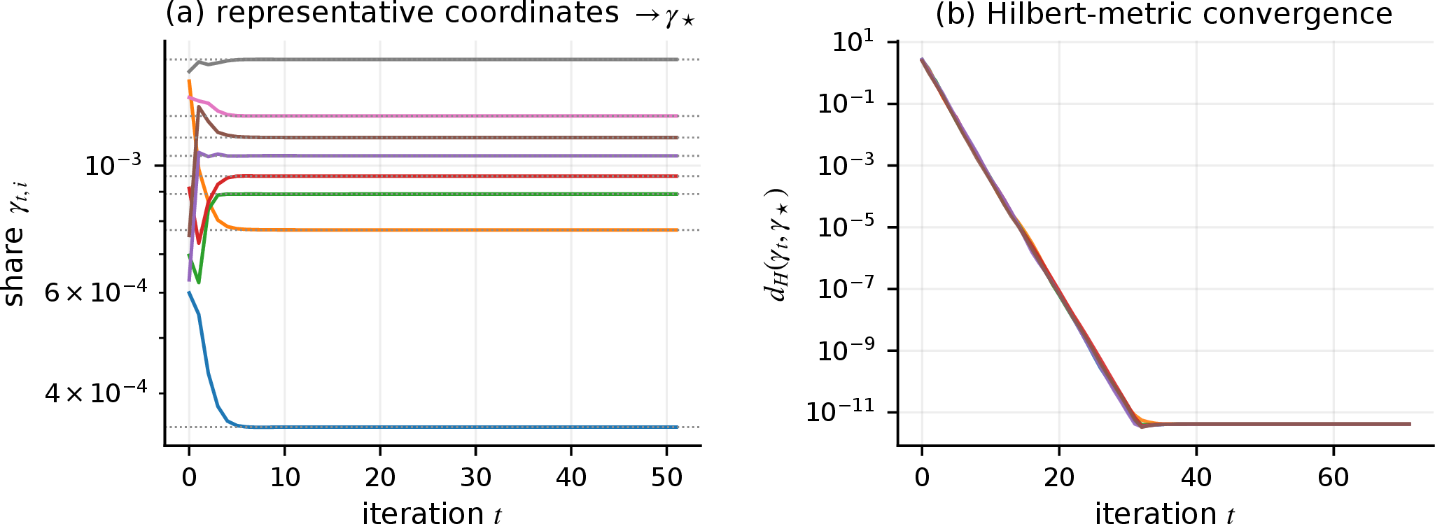
Figure 2 records a second numerical check: the dependence on the forcing rate. When mixing is fast relative to forcing, the selected profile is close to the \(\pi\)-free benchmark \(P_\theta(v)\), where \(v\) is the Perron response of the transport matrix. In the displayed example the distance is approximately linear in \(\pi/(1-|\lambda_2|)\). This is not a claim that \(\pi\) is always irrelevant. The approximation is controlled when the forcing rate is small compared with the spectral mixing gap; on a slowly mixing or modular graph the longer resolvent memory can matter substantially. The point is narrower: once the response has effectively mixed over the forcing horizon, the normalized fixed point is controlled mainly by the response profile and by \(\theta\), rather than by the absolute rate at which total mass grows.
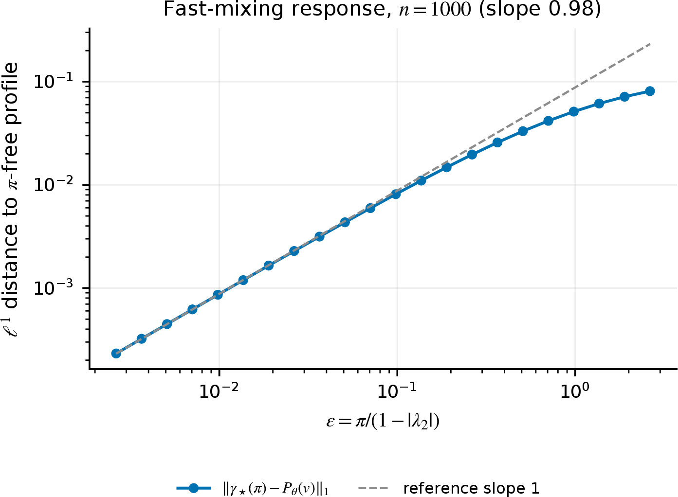
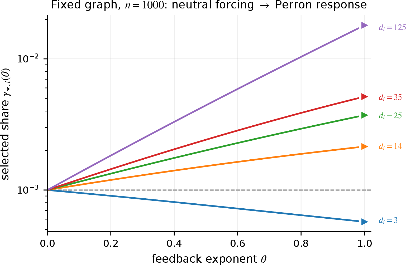
Figure 3 shows the same fixed point along the positive feedback branch on one graph. At \(\theta=0\) the forcing is uniform. As \(\theta\) increases, the profile moves continuously toward the Perron response: high-response, high-degree nodes rise, while low-response nodes lose share. This figure is deliberately simpler than a full phase diagram. It shows the central mechanism in the stable regime: the feedback exponent reweights a fixed response field rather than changing the graph.
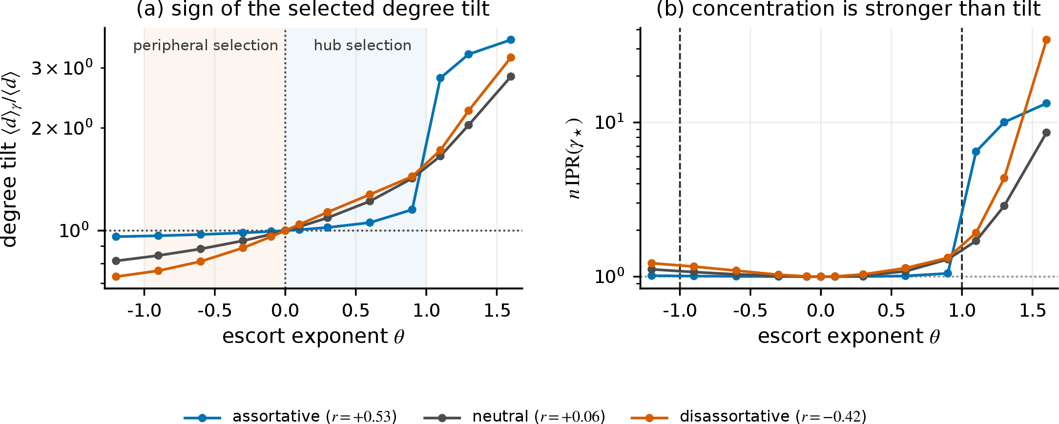
The sign law is shown in Figure 4. The tilt is measured by the mass-weighted mean degree \(\langle d\rangle_\gamma=\sum_i\gamma_{\star i}\,d_i\) divided by the unweighted mean \(\langle d\rangle=n^{-1}\sum_i d_i\), a ratio that equals one for the uniform profile. Sweeping \(\theta\) through zero, this tilt crosses its neutral value at \(\theta=0\). For \(\theta>0\) the profile tilts toward hubs; for \(\theta<0\) it tilts toward the periphery. Rewiring the same degree sequence changes the strength of the effect. Disassortative and neutral networks produce a stronger tilt, while a strongly assortative network keeps the two ends of the degree sequence more separated and hence closer to uniform in the contracting window. For \(|\theta|\ge1\) the contraction certificate of Section 3 no longer applies; on these instances the iteration of \(T\) still settled to a numerically stationary profile, and the plotted points describe that profile; no uniqueness is claimed there. The rise of the IPR outside that window is a finite-network observation. In particular, an IPR increase on the negative branch does not contradict Proposition 4: it need not survive along graph sequences with an extensive low-response class.
Figures 5 and 6 test the participation-ratio prediction. For a degree-tail exponent \(\alpha=2.5\), the predicted threshold is \(\theta_2=(\alpha-1)/2=0.75\). Below this value the IPR follows the dispersed scaling \(n^{-1}\) over the available size range. Above it, the decay becomes slower. The finite-size slope reported in these figures is the logarithmic derivative \(d\log\operatorname{IPR}/d\log n\), estimated from log–log fits over windows of consecutive sizes. Repeating the experiment for different tail exponents moves the observed kink in the expected direction. The transition is a finite-size crossover, not a sharp singularity at the sizes simulated, but the running exponent tracks the predicted threshold.

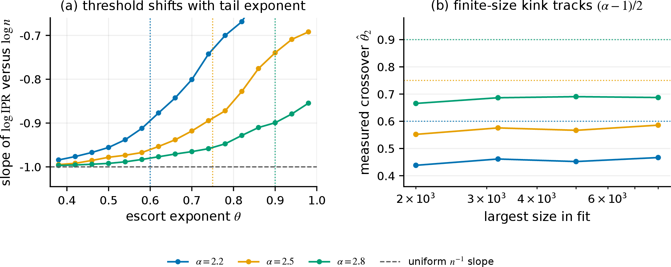
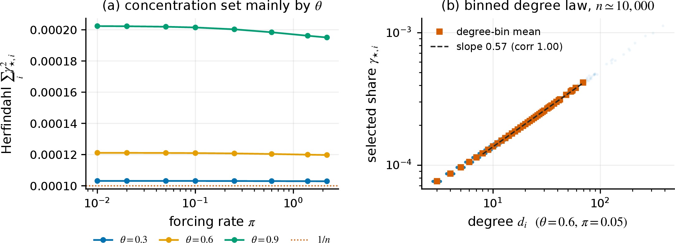
Figure 7 gives a more local check of the degree-class approximation. The Herfindahl index—the moment \(\mathcal{M}_2(\gamma_\star)=\sum_i\gamma_{\star i}^2\) of Section 5, identical to the IPR—changes strongly with \(\theta\) and weakly with \(\pi\) in the fast-mixing/slow-forcing regime, in agreement with the view that feedback exponent and response heterogeneity set the shape. The degree-binned profile follows a clear power law, while pointwise values remain noisy. The fitted exponent sits slightly below \(\theta\) itself, which is what the reduced law 24 leads one to expect: binned shares obey \(\eta(k)\propto\varphi(k)^\theta\), so the measured log–log slope is \(\theta\) times the local slope of the transported response against degree, and the primitive regularization together with residual degree correlations bends that local slope slightly away from strict proportionality \(\varphi(k)\propto k\). This is the correct interpretation of the mean-field degree law: it is a statement about binned response classes and tails, not a promise that every vertex is determined by its degree alone.
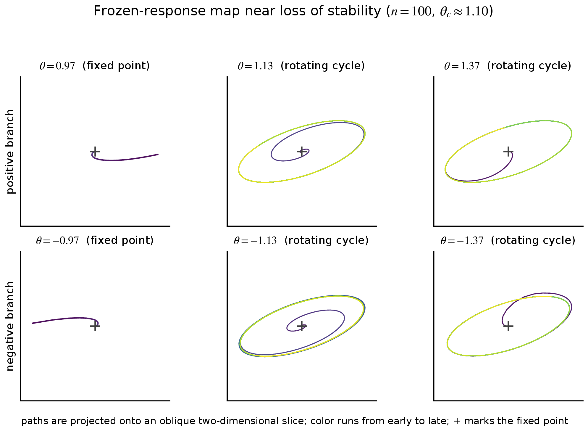
Finally, Figure 8 illustrates the iteration of the frozen-response map after its attracting fixed point loses local stability. On a directed-cycle network with a small positive background, the reverse kernel is non-reversible and the leading local multipliers form a complex pair. Numerically, beyond the crossing the map orbit settles onto a rotating wave. This calculation is not a stability theorem for the original finite-memory recursion outside Theorem 1, and it is not part of the heavy-tail condensation proof. It is included only to show that the same feedback law can select a steady profile in one regime and cyclic redistribution in another.
Taken together, the experiments support the intended reading of the theory. The fixed point is robust in the contracting regime; the sign of \(\theta\) chooses the direction of the phase; assortativity controls its strength; and the IPR transition is a tail effect, not merely a visual increase in inequality. The simulations also show the limits of the asymptotic statements. Degree-class laws are accurate after binning but noisy pointwise, and finite graphs display crossovers rather than sharp thresholds. The bifurcation panel is likewise a map-level illustration rather than evidence about the full recursion beyond the sufficient convergence condition.
These finite-size qualifications are part of the result rather than a nuisance. A real network has a largest hub, a finite peripheral class, and non-universal correlations. The theorem predicts how the diagnostics scale along graph sequences; it does not claim that a single finite graph contains a sharp thermodynamic singularity. For empirical use, the safest procedure is therefore to report several diagnostics together: degree tilt or response tilt, IPR, effective support, and top-share. Agreement among them is strong evidence for true localization, while disagreement usually indicates a broad tilted phase.
7 Conclusion↩︎
We have studied an open transport process in which a fixed network mixes mass while feedback chooses where new mass enters. After total growth is removed, the profile is governed by a nonlinear Perron–Frobenius fixed point. The useful contraction estimate is almost elementary: the positive network response contracts Hilbert’s projective metric and the escort map rescales it by \(|\theta|\). Under explicit mixing–forcing conditions, the resulting fixed point attracts every admissible orbit.
The physical content is that heavy-tailed heterogeneity does not by itself decide where mass goes. The sign of the feedback exponent decides which end of the response field is selected. Positive feedback draws mass toward high-response nodes, which are often the hubs. Negative feedback shifts it in the opposite direction, toward nodes with low response. Network assortativity and mixing then determine how strong the tilt is and whether it becomes genuine localization.
There is also a diagnostic lesson. Broad degree tilt, anomalous IPR scaling, and true few-node localization are different forms of concentration. The heavy-tail calculation shows where the IPR first leaves the uniform scaling, while the zero-temperature limits show why the negative branch can remain broad even under strong anti-reinforcement. The separation matters on finite networks, where a visibly unequal profile need not be a condensate in the participation-ratio sense.
The analysis also gives a useful practical rule. On a finite network one should not identify condensation from a single plot or a single inequality measure. The response tilt shows whether mass is drawn toward high- or low-response nodes. The IPR and entropy indicate whether the favored group is genuinely small. Degree-binned averages then show whether the apparent centrality pattern extends across the network or is driven by only a few exceptional nodes. The warning applies with most force to anti-condensation, where the selected low-response class may be extensive.
The model is intentionally minimal. It leaves several extensions open: random forcing, time-dependent networks, conserved components, and empirical estimation of the feedback exponent from data. A complementary direction is to study standing-stock and edge-current observables after the selected injection profile has been identified, especially on directed networks near a loss of fixed-point stability.
Supplementary material↩︎
The Supplementary Material contains a modular proof of the convergence criterion with a checkable form of the small-gain condition (Sec. S2), a precise slow-forcing limit for the resolvent response (Sec. S3), the truncated-moment calculation behind the participation-ratio crossover (Sec. S4), the reverse-kernel derivation together with standing-stock and current observables (Sec. S5), and numerical implementation notes with a table of the reported parameters (Sec. S6).