1 Introduction↩︎

Given a base function \(f\), consider the task of computing its \(n\)-fold product function \(f^n(x_1, \ldots, x_n) := (f(x_1), \ldots, f(x_n)).\) A natural approach is to apply an optimal algorithm for \(f\) independently to each input, using \(n\) times the cost of computing a single instance. But is this optimal?

This problem is known as the direct-sum question, and it is among the most central in computational complexity theory. It has been studied extensively across a variety of computational models such as circuit complexity [1]–[4], communication complexity [5]–[10], information complexity [7], [11], [12], and query complexity [13]–[18], to name just a few.

In parallel, another line of research investigates the complexity of composition functions \(g \circ f^n\). For an arbitrary “outer gadget” \(g\), the optimal bounds (i.e. proportional to the complexity of \(f\) and \(g\)) are known under certain complexity measures such as deterministic query complexity [19]–[21] and quantum query complexity [22], [23]. However, for general complexity measures, a starting point is to understand the complexity of \(g\circ f^n\) when \(g\) is an explicit gadget. That is, to study how the cost of computing \(g \circ f^n\) scales with the cost of computing \(f\) and with \(n\), for a specific \(g\). Naively, one could still compute \(f\) on each input and then apply \(g\) to the outputs. In the spirit of the direct-sum question, we may ask whether this simple strategy is optimal.

Besides the identity gadget for which 1 becomes the direct-sum problem, perhaps the most extensively studied gadget is the \(\mathsf{XOR}\) function, which computes the parity of its \(n\)-bit input. Results of this type, often called the XOR lemma, have also been well-established in various computational models, e.g. [4], [7], [24]–[28]. Beyond the XOR lemma, however, our understanding of 1 is relatively limited and is mostly contained to query complexity with respect to the \(\mathsf{OR}\), \(\mathsf{GapOR}\), and \(\mathsf{MAJ}\) gadgets [29]–[31].

1.0.0.1 Gap-Majority Lemma.

We focus on the gap-majority gadget which computes the majority of \(n\) binary inputs if the bias is \(\Omega(\sqrt{n})\). Formally, define the gadget \(\mathsf{GapMAJ}_n: \{\pm1\}^n \rightarrow \{\pm1\}\) as: \[\begin{align} \mathsf{GapMAJ}_n(z_1,\ldots,z_n) := \begin{cases} +1 & \text{if } \sum_{i=1}^{n} z_i \geq 0.01 \sqrt{n}, \\ -1 & \text{if } \sum_{i=1}^{n} z_i \leq -0.01 \sqrt{n}. \end{cases} \end{align}\] Given a base function \(f: \mathcal{X} \rightarrow \{\pm 1\}\), we aim, with probability at least \(0.99\), to compute the composite function \[\begin{align} \mathsf{GapMAJ}_n \circ f^n(X_1,\ldots,X_n) := \begin{cases} +1 & \text{if } \sum_{i=1}^{n} f(X_i) \geq 0.01 \sqrt{n},\\ -1 & \text{if } \sum_{i=1}^{n} f(X_i) \leq -0.01 \sqrt{n}. \end{cases} \end{align}\]

At first glance, it is even unclear what the naive approach should be. One natural attempt is as follows: suppose there exists an algorithm \(\mathcal{A}\) that computes \(f(X)\) with error \(1/(100n)\). We can estimate \(\sum_{i=1}^n f(X_i)\) by applying \(\mathcal{A}\) independently to each input and summing the results. By the union bound, this recovers the exact sum with probability \(0.99\), yielding the correct output.

However, we can exploit the generous margin of \(\pm 0.01\sqrt{n}\) to do better. Suppose \(\mathcal{A}\) computes \(f(X)\) with a small constant error, say \(10^{-100}\). By standard concentration bounds, the estimate of \(\sum_{i=1}^n f(X_i)\) is within \(\pm 10^{-10}\sqrt{n}\) of the true value with high constant probability, which suffices to distinguish between the “\(+1\)” and “\(-1\)” cases of \(\mathsf{GapMAJ}_n \circ f^n\). Thus, the naive approach requires only \(n\) times the resources needed to compute \(f\) with low “constant” error.

With this benchmark established, the natural question is whether such linear scaling is optimal. We refer to this as the gap-majority lemma question.

1.1 Main Results↩︎

We study the gap-majority lemma in the realm of two-player randomized communication. In this setting, two players hold separated parts of inputs of a function \(f: \mathcal{X} \times \mathcal{Y} \to \{\pm 1\}\), namely Alice has \(X \in \mathcal{X}\), Bob has \(Y \in \mathcal{Y}\), and they exchange a (possibly randomized) sequence of messages to compute \(f(X, Y)\) with reasonable constant success probability. The scheme by which the players exchange messages and produce an output is called a communication protocol.

Correspondingly, the gap-majority composition problem of a base function \(f\), denoted \(\mathsf{GapMAJ}_n \circ f^n\), assigns \(X = (X_1, \ldots, X_n)\) to Alice and \(Y = (Y_1, \ldots, Y_n)\) to Bob. The players then must, with high constant probability, jointly compute \[\begin{align} \mathsf{GapMAJ}_n \circ f^n(X_1,\ldots,X_n, Y_1,\ldots,Y_n) := \begin{cases} +1 & \text{if } \sum_{i=1}^{n} f(X_i, Y_i) \geq 0.01 \sqrt{n}, \\ -1 & \text{if } \sum_{i=1}^{n} f(X_i, Y_i) \leq -0.01 \sqrt{n}. \end{cases} \end{align}\]

Our main result establishes the gap-majority lemma in this setting when the notion of cost is internal information, denoted \(\IC(\cdot)\), which quantifies the amount of information revealed by the protocol.³ In particular, we show that computing \(\mathsf{GapMAJ}_n \circ f^n\) requires \(\Omega(n)\) times the information needed to compute a single instance of \(f\), up to a small additive loss.

We make a few remarks regarding this theorem. First, we may even relax the range of \(f\) so that it only requires \(f(x,y) \in \{\pm 1\}\) over the support of \(\mu\). Second, the \(O(1)\)-additive “loss” in information cost is in fact unavoidable. To see this, consider the simple example \(f(x,y) := x - y\) with respect to the input distribution \(\mu\) which is uniform over \((x,y) \in [10^4] \times [10^4]\) conditioned on \(x - y \in \{\pm 1\}\). In this example, any protocol \(\eta\) that computes \(f(x,y)\) over \(\mu\) with probability \(0.501\) must reveal \(\Omega(1)\) bits of information.⁴ On the other hand, there is a deterministic protocol \(\pi\) which computes \(\mathsf{GapMAJ}_n \circ f^n\) while communicating only \(O(\log{n})\) bits: Alice sends the value \(\sum_{i=1}^n x_i\) to Bob, who then can compute \(f^{+n}(x_1,\ldots,x_n,y_1,\ldots,y_n) = \sum_{i=1}^n x_i - \sum_{i=1}^n y_i\) and decides if it is at least \(0.01\sqrt{n}\) or at most \(-0.01\sqrt{n}\).

More importantly, although the \(O(1)\)-additive loss is small and oftentimes negligible, it comes at the expense of round complexity: in our proof of 3, the protocol \(\eta\) uses \(O(\log n)\) more rounds than \(\pi\) does. Such a mismatch in the number of rounds can be undesirable in certain applications. For example, a standard approach to proving single-pass streaming lower bounds is to reduce a streaming algorithm to a one-way communication problem and then prove a communication lower bound. The one-way restriction is typically the primary source of hardness, and as a result, losing an additional \(O(\log n)\) rounds in the reduction may lead to a significantly weaker lower bound.

To remedy this, we also provide a variant of the gap-majority lemma which also preserves the number of rounds!

It is helpful to view 4 as a counterpart to 3: one can preserve the number of rounds at the cost of \(O(\log n)\) extra bits, as opposed to \(O(1)\) in the unbounded-round setting. It remains an open question whether the best of both worlds can be achieved; that is, whether there exists an \(r\)-round protocol \(\eta\) with only \(O(1)\) bits of information loss. We conjecture this is possible.

Finally, we emphasize that both of our gap-majority lemmas are strong, in the sense that they achieve asymptotic optimality in both the scaling of information cost and the error tradeoffs, as witnessed by the naive approach. This makes \(\mathsf{GapMAJ}\), to our knowledge, only the third explicit gadget known to admit a strong composition theorem in two-player communication, following the identity gadget (i.e., the direct-sum theorem) [7], [9] and the XOR gadget (i.e., the XOR lemma) [25], [27], [28].

1.2 Implication↩︎

1.2.0.1 Why Gap-Majority?

Gap-type problems have long served as fundamental tools for proving lower bounds for approximation problems. The underlying reason is simple yet powerful: many approximation tasks can be reduced to distinguishing between two well-separated cases of a decision problem—precisely the scenario highlighted by a “gap” function.

A particularly important instance of the gap-majority lemma arises when the base function is \(f: \{\pm 1\} \times \{\pm 1\} \rightarrow \{\pm 1\}\) is the XOR function (with basis change), defined as \(f(x,y) := xy\). In this case, the composition \(\mathsf{GapMAJ}_n \circ f^n\) translates to the well-celebrated Gap-Hamming problem in the two-player communication setting: Alice and Bob each hold a vector in \(\{\pm 1\}^n\), and their goal is to decide whether the inner product between their vectors is at least \(0.01\sqrt{n}\) or at most \(-0.01\sqrt{n}\). The problem was formally introduced by Indyk and Woodruff [32] who also proved the optimal lower bound of \(\Omega(n)\) in one-way communication. The complete unbounded round lower bound, however, only arrived a decade later [33]–[35]. Regardless, since its inception (or even prior to that), Gap-Hamming has quickly become a cornerstone of communication complexity which, both explicitly and implicitly, leads to countless lower bounds across multiple computational models [32], [36]–[41].

1.2.0.2 A new framework for proving lower bounds.

While the Gap-Hamming problem alone has already yielded a rich array of lower bounds results, our gap-majority lemmas provide an even more generic framework for amplifying the hardness of “any” base decision problem \(f(x,y)\) into the hardness of an associated approximation problem \(f^{+n}(x_1,\ldots,x_n,y_1,\ldots,y_n) := f(x_1,y_1) + \ldots + f(x_n,y_n)\). By a standard reduction from our main results (3 and 4), we obtain the following corollaries.

These corollaries yield a clean framework for proving communication lower bounds for approximation problems. Conceptually, this framework plays a role analogous to that of direct-sum theorems, which lift lower bounds from a base problem to its \(n\)-fold product version, a technique that has seen frequent success in the literature. In our setting, however, the emphasis is on systematically lifting hardness from a decision problem to an approximation problem via the following recipe:

1. Reduction. Show that an algorithm for approximating the target problem \(\mathcal{P}\) can be used to approximate \(f^{+n}\) within \(\pm 0.01\sqrt{n}\), for some appropriate choices of a base decision problem \(f\) and \(n \in \mathbb{Z}^+\).

2. Base lower bound. Prove that any protocol that decides \(f\) with probability \(0.501\) requires at least \(\mathcal{I}\) bits of information.

Then, by applying either 1 or 2 as a black box, we obtain an information and communication lower bound of roughly \(\Omega(n \cdot \mathcal{I})\) for the approximation problem \(\mathcal{P}\).

1.2.0.3 Lower Bound Applications.

For completeness, we showcase the power of the gap-majority lemma through a few of its quick applications.

• Communication Complexity of Gap-Hamming. As previously noted, the Gap-Hamming problem is a particularly important instance of the gap-majority composition. While the optimal communication lower bound of \(\Omega(n)\) bits has long been established [33]–[35], it is only natural to recover such bound through the lens of our gap-majority framework. We present this proof in 6.1. Indeed, treating the gap-majority lemma as a “black-box” amplification tool, our proof proceeds through a very simple and clean reduction to the classical set-disjointness problem.

• Streaming Complexity of Triangle Counting. Given an \(n\)-vertex, \(m\)-edge graph with \(T\) triangles presented as an edge-arrival stream, the triangle counting problem asks for a \((1 \pm \varepsilon)\)-approximation to the number of triangles in \(G\), that is, to output an estimate \(\widetilde{T}\) satisfying \(|\widetilde{T}-T|\leq \varepsilon T\). A naive solution is to store the entire graph and use \(\widetilde{O}(m)\) space. This bound turns out to be beatable subjected to the range of parameters. For instance, Buriol et al. [42] gave a sampling-based algorithm using \(\widetilde{O}\left(\frac{mn}{\varepsilon^2 T}\right)\) space, surpassing the naive algorithm when \(G\) has many triangles.

  To this end, we show, via gap-majority framework, that these two quantitative upper bounds are jointly optimal: any randomized single-pass streaming algorithm for \((1 \pm \varepsilon)\)-approximate triangle counting requires \(\Omega\left(\min\left\{m,\;\frac{mn}{\varepsilon^2 T}\right\}\right)\) bits of space, for a reasonable range of \(T\). Prior to our work, the best-known space lower bound is \(\Omega\left(\min\left\{m,\;\frac{mn}{T}\right\}\right)\) bits due to Braverman, Ostrovsky, and Vilenchik [43].⁵ Hence, our contribution lies in bringing up the missing \(1/\varepsilon^2\) factor of these existing lower bounds. We present this proof in 6.2.

For brevity, we defer the extended introduction and complete lower bound proof of both problems to 6. We leave it as an intriguing direction whether our gap-majority lemmas can be applied (either in a black-box or white-box manner) to derive lower bounds beyond those listed here.

2 Preliminaries↩︎

2.0.0.1 Notations.

For a base function \(f\) with real-valued outputs, we define its \(n\)-fold summation as \(f^{+n}(X_1,\ldots,X_n) := f(X_1) + \ldots + f(X_n)\). We may occasionally write \(f^{+n}\) simply as \(f^{+}\), omitting the number of summands.

Following standard convention in probability, we use uppercase letters to denote random variables and lowercase letters for their realization. For a joint distribution \(\pi\) over multiple random variables, \(\pi(A)\) denotes the marginal distribution of \(A\), and \(\pi(a)\) its probability mass at \(A=a\). Similarly, \(\pi(A \mid B)\) denotes the conditional distribution of \(A\) given \(B\), and \(\pi(A \mid b)\) the distribution of \(A\) conditioned on \(B=b\). We write \(\mathbb{E}[A]\) and \(\textrm{Var}[A]\) for the expectation and variance of \(A\), respectively, and use subscripts to indicate the variable of integration, e.g. \(\mathbb{E}_A[f(A)]\). When clear from context, we omit the subscript. We will also frequently use the following simple fact which can be proven via the Cauchy-Schwarz inequality.

2.0.0.2 Communication Protocol.

We adopt the distributional view of randomized communication protocols. A protocol \(\pi\) is represented as a joint distribution \((X,Y,M,R)\), where \((X,Y) \sim \mu\) is the input pair given to Alice and Bob, \(M= (M_1,M_2,\ldots)\) is the transcript, and \(R\) denotes public randomness. The protocol operates as follows. Alice and Bob receive inputs \((X,Y) \sim \mu\) respectively. Assume Alice speaks first. She draws the first message \(M_1 \sim \pi(M_1 \mid XR)\) and sends it to Bob. Bob then draws the second message \(M_2 \sim \pi(M_2 \mid M_1YR)\) and sends it back to Alice. The communication between players goes on as needed, and thereby forms a transcript \(M\). Without restricting the number of rounds (i.e. the number of messages), if the protocol is designated to compute a function \(f\), we may assume that the final message of the protocol is the players’ answer to \(f(X,Y)\). We can always enforce this assumption, e.g. if Alice is responsible for computing \(f(X,Y)\), she simply sends an extra (short) message to Bob indicating the answer. The communication cost of \(\pi\), denoted \(\mathsf{CC}(\pi)\), is measured by the worst-case length of the message \(M\).

2.0.0.3 Protocol with Bounded Rounds.

A special case of communication protocols occurs when we restrict the number of rounds of communication to \(r\). We may assume wlog that \(r\) is odd. In this setting, Alice and Bob can communicate for \(r\) rounds and towards the end of their conversation, Bob is asked to produce an answer to \(f(X,Y)\). Note that Alice may not know this answer. We denote an \(r\)-round protocol by \(\pi = (X,Y,M,A,R)\), where \(M = (M_1,\ldots,M_r)\) is the sequence of \(r\) messages, \(R\) is shared public randomness, and \(A\) is Bob’s output computed from \(MYR\). Denote \(\mathcal{A}\) to be the space of all possible answers \(A\). For instance, we use \(\mathcal{A} = \{\pm 1\}\) for decision problems.

2.0.0.4 Information Cost.

The information cost of a protocol \(\pi = (X,Y,M,R)\) is given by the quantity: \[\IC(\pi) := I(M:X \mid YR) + I(M:Y \mid XR)\] where \(I(\cdot:\cdot)\) denotes mutual information. It is helpful to interpret \(\mathsf{IC}(\pi)\) as the amount of information that \(\pi\) reveals about the players’ inputs. To see this, from Alice’s view at the end of \(\pi\), she learns the transcript \(M\) while already knowing her own input \(X\) and randomness \(R\). Hence, the term \(I(M:Y \mid XR)\) quantifies the information she gains about Bob’s input \(Y\) after running \(\pi\).

The information cost is also defined by the same quantity even if \(\pi = (X,Y,M,A,R)\) is bounded-round. Note that we always have \(\mathsf{IC}(\pi) \leq \mathsf{CC}(\pi)\).

2.0.0.5 Rectangle Property.

Rectangle property is one of the defining features of communication protocols. It asserts that in a communication protocol whose inputs consist of multiple coordinates drawn from a product distribution, conditioned on a set of disjoint inputs and the message \(M\) (and randomness \(R\)), the remaining portions of players’ input are independent.

3 Approach↩︎

In this section, we outline the roadmap toward our two main results (3 and 4), with the proof of key technical lemmas deferred to later sections.

3.1 Gap-Majority Lemma↩︎

Our proof of 3 proceeds by introducing a new measure called the observer’s variance.

In words, the observer’s variance measures, from the perspective of an external observer, the uncertainty of \(f(X,Y)\) after the protocol concludes. Particularly from an external view, they see only the transcript \(M\) and the public randomness \(R\), but not the players’ private inputs. For each realization of \(MR\), the observer considers the posterior distribution of \(f(X,Y)\) conditioned on these values and evaluates the uncertainty \(f(X,Y)\) via its variance. Averaging over all \(MR\) then yields \(\Phi_{\textrm{obs}}(\pi @ f)\), representing the expected variance of \(f\) given the protocol’s external view.

With this definition in place, we now state the two key ingredients that together establish the gap-majority lemma (3).

3.1.0.1 Ingredient #1: Gap-majority implies low variance.

We first show that any protocol that computes gap-majority with high constant probability must admit low linear observer’s variance, say at most \(0.99n\). This phenomenon was previously observed in a streaming setting by Braverman, Garg, and Woodruff [45], who showed that any streaming algorithm capable of computing the exact majority necessarily has low linear variance. For our purposes, we strengthen this result to the communication setting for gap-majority composition, as stated in [lem:gapmaj95then95low95variance]. We emphasize that our proof follows closely from [45] to which we defer to the appendix.

3.1.0.2 Ingredient #2: A new direct-sum theorem.

To motivate our second ingredient, it is best to discuss the following toy question: How should the information cost and observer’s variance for \(f^{+n}\) scale relative to those for a single instance of \(f\)?

In an easy direction, suppose that we have a protocol \(\theta\) for computing \(f\) using \(\mathcal{I}\) bits of information, and with variance \(\sigma^2\). We can then employ a naive approach by applying \(\theta\) on the \(n\) pairs of inputs independently, and then sum up the answers. This approach simply use \(n \cdot \mathcal{I}\) bits of information. But how does the variance of \(f^{+n}\) scale? The key observation is that each execution of \(\theta\) is independent; thus, we can directly sum up the variance to \(n\sigma^2\). Notice that the optimality question of this naive protocol is exactly the direct-sum problem: we may ask if the scaling factor \(n\) of information costs and variances are tight, or even stronger, are they simultaneously tight?

Our second ingredient is a direct-sum theorem that answers this question in an affirmative, barring a small additive loss. We state the result here and present its proof in 4.

Crucially, we view this lemma as a central technical contribution of our work. Note that unlike [lem:gapmaj95then95low95variance], the condition \(\mathbb{E}_\mu[f(x,y)] = 0\) is not required here. Whether [lem:main95lemma] has further applications beyond the gap-majority setting, in our opinion, is a direction worth exploring.

As a remark, [lem:main95lemma] extends naturally to the setting where \(f\) maps to the interval \([-d,d]\) and \(\Delta \in (0,d^2)\) for some \(d \in \mathbb{R}^+\). In this case, the statement remains the same except that the additive loss in the information cost becomes \(O(1+\log{\frac{d^2}{\Delta}})\). For brevity, we omit this proof.

3.1.0.3 Putting all together.

We now combine both ingredients to recover the gap-majority lemma.

3.2 Round-Preserving Gap-Majority Lemma↩︎

We now sketch the proof of 4 which is an analogue of 3 restricted to the class of \(r\)-round communication. As outlined in 2, we may assume that \(r\) is odd and write an \(r\)-round protocol as \(\pi = (X,Y,M,A,R)\), where \(M = (M_1,\ldots,M_r)\) is the sequence of \(r\) messages, and \(A\) is the output produced solely by Bob after the \(r\) rounds of communication. Since Bob can no longer communicate the answer \(A\) back to Alice (otherwise it would have taken an extra round), the observer’s variance is no longer a reliable proxy for distributional error. To accommodate this, we refine the notion of variances by distinguishing it into two types: observer’s and Bob’s.

In principle, the observer’s variance remains the same as before, only now adapted to the bounded round setting: an external observer sees \(MRA\) and measures the expected variance of \(f(X,Y)\) conditioned on this view. Bob’s variance, however, is new: it quantifies the expected variance of \(f(X,Y)\) from Bob’s perspective at the end of the protocol, given that he sees \(MRAY\). When \(f\) is a decision problem, this quantity turns out to be related to the distributional error.

Following the same avenue, we introduce the two key ingredients tailored to \(r\)-round communication. The variance bound ([lem:gapmaj95then95low95variance951way]) parallels [lem:gapmaj95then95low95variance], and for brevity, we omit its proof. The round-preserving direct-sum theorem ([lem:main95lemma95oneway]) is analogous to [lem:main95lemma], except for a slightly larger additive loss in the information cost. Notably, the proof of [lem:main95lemma95oneway] is more technically involved than that of [lem:main95lemma] due to the round constraint. We present this proof in 5.

We conclude by combining [lem:gapmaj95then95low95variance951way] and [lem:main95lemma95oneway] to prove our second main result.

3.3 Proof Outline↩︎

Three proofs are deferred from this section. The proof of [lem:gapmaj95then95low95variance] is provided in Appendix 8. The proof of [lem:main95lemma] and [lem:main95lemma95oneway] are provided in 4 and 5 respectively.

4 Direct-Sum for Variance and Information↩︎

In this section, we prove [lem:main95lemma], thereby completing the proof of the gap-majority lemma (3). We adopt the setting of the lemma: let \(f: \mathcal{X} \times \mathcal{Y} \rightarrow \{\pm 1\}\) be an arbitrary base function, and let \(\mu\) be an arbitrary input distribution. Denote by \(\pi = (X,Y,M,R)\) a protocol over the product distribution \(\mu^n\), where \(X = (X_1,\ldots,X_n)\) and \(Y = (Y_1,\ldots,Y_n)\) with each \((X_i,Y_i)\) drawn independently from \(\mu\). Let \(\Delta \in (0,1)\) be an arbitrary additive loss parameter.

A key component of our proof is an adaptation of the protocol decomposition technique [25], [28]. Given a protocol \(\pi\) operating on \(n\) input pairs drawn according to \(\mu^n\), a decomposition is a procedure that yields two smaller-yet-meaningful subprotocols, \(\pi_0\) and \(\pi_1\), each operating on \(n/2\) input pairs drawn according to \(\mu^{n/2}\). As employed in [25], [28], their decompositions are carefully designed to trace how information is distributed across different parts of the input. A key distinction in our work is that our decomposition is tailored to handle not only the distribution of information, but also the distribution of observer’s variances across all the \(n\) input pairs.

Particularly, we describe the protocols \(\pi_0\) and \(\pi_1\) (yielded by our decomposition) in [pi0,pi1]. Each protocol operates on \(n/2\) pairs of input, denoted \((X', Y')\), drawn from \(\mu^{n/2}\).

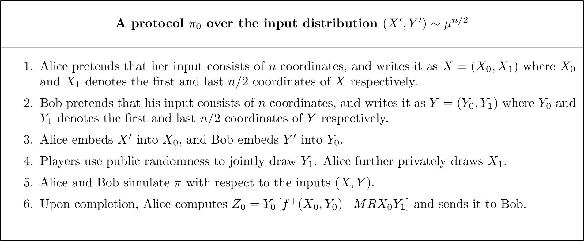
Equivalently, we may adopt the following distributional view of each protocol. Note that we write \((M,Z_i)\) to denote a transcript \(M\) followed by an extra message \(Z_i\).

• \(\pi_0 = (X_0, Y_0, (M,Z_0), RY_1)\) where \(Z_0 = \underset{Y_0}{\mathbb{E}}\left[f^+(X_0, Y_0) \mid MRX_0Y_1\right]\) computable by Alice. This is because \(Z_0\) is a deterministic function of \(MRX_0Y_1\) in which she knows by the end of \(\pi\).

• \(\pi_1 = (X_1, Y_1, (M,Z_1), RX_0)\) where \(Z_1 = \underset{X_1}{\mathbb{E}}\left[f^+(X_1, Y_1) \mid MRX_0Y_1\right]\) computable by Bob. This is because \(Z_1\) is a deterministic function of \(MRX_0Y_1\) in which he knows by the end of \(\pi\).

For the moment, we assume that Alice and Bob can communicate the exact values of \(Z_0\) and \(Z_1\), and that these variables take values from some discrete space \(\mathcal{Z}\). Of course, this assumption does not necessarily hold in general. The purpose of this simplification is purely expository; we will remove this assumption shortly, incurring only minor losses.

The primary advantage of this decomposition is that it enables a clean algebraic decomposition of our two key measures of interest: the information cost and the observer’s variance.

4.0.0.1 Decomposition of Information Costs.

We first show that under the decomposition, the information costs decompose linearly with some small additive loss.

4.0.0.2 Decomposition of Variances.

Next, we show that the observer’s variance decomposes linearly. We begin by reinterpreting the observer’s variance of each protocol.

As a result, we obtain a linear decomposition of observer’s variances.

4.0.0.3 Lifting the assumptions about \(Z_0, Z_1\).

Recall that in the protocol \(\pi_0\), we require Alice to compute \(Z_0 = \underset{Y_0}{\mathbb{E}}\left[f^+(X_0, Y_0) \mid MRX_0Y_1\right]\) and communicate it exact value to Bob. To lift the assumptions, we now instead let Alice sends the value of \(Z_0^2\) rounded down to the nearest multiple of \(\frac{\Delta}{32}\). We denote such value by a random variable \(\hat{Z}_0^2\). Bob also replaces \(Z_1\) with \(\hat{Z}_1^2\), defined analogously. The implications of such rounding scheme are as follows.

• Observe that the range of \(Z_0^2\) and \(Z_1^2\) is \([0,n^2]\). This allows us to set a discrete space \(\mathcal{Z}\) to be \(\{0, \frac{\Delta}{32}, \ldots \frac{\Delta}{32}, \ldots, \frac{\Delta}{32} \cdot \lfloor n^2 \cdot \frac{32}{\Delta}\rfloor\}\). As a result, \(|\mathcal{Z}| = O(\frac{n^2}{\Delta})\). Plugging this into 7, the decomposition of information costs may incur an additive loss of at most \(O(\log{\frac{n}{\Delta}})\) bits.

• In the variance analysis of 8, the exact value of \(Z_0^2\) (and symmetrically, \(Z_1^2\)) was only used in 2 . Replacing \(Z_0^2\) by \(\hat{Z}_0^2\) introduces at most an additive error of \(\frac{\Delta}{32}\) to \(\Phi_{\textrm{obs}}(\pi_0 @ f^{+n/2})\). The same argument applies to \(\pi_1\), giving a total additive loss of at most \(\frac{\Delta}{16}\) to the combined variance decomposition.

In summary, replacing the exact values \(Z_0\) and \(Z_1\) by their squared and rounded counterparts \(\hat{Z}_0^2\) and \(\hat{Z}_1^2\) preserves the linear decomposition properties, at the cost of an additive \(O(\log \tfrac{n}{\Delta})\) in information and \(\tfrac{\Delta}{16}\) in variance. This yields the following decomposition lemma.

We are now ready to prove the main result of this section.

5 Round-Preserving Direct-Sum for Variance and Information↩︎

We now prove [lem:main95lemma95oneway], thereby completing the proof of the round-preserving gap-majority lemma (4). We adopt the setting of the lemma: let \(f: \mathcal{X} \times \mathcal{Y} \rightarrow \{\pm 1\}\) be an arbitrary function, and let \(\mu\) be an arbitrary input distribution. Denote by \(\pi = (X,Y,M,A,R)\) an \(r\)-round protocol over the product distribution \(\mu^n\), where \(X = (X_1,\ldots,X_n)\) and \(Y = (Y_1,\ldots,Y_n)\) with each \((X_i,Y_i)\) drawn independently from \(\mu\). We also write \(M = (M_1,\ldots,M_r)\) as a sequence of \(r\) messages. We may assume \(r\) is odd so that Alice sends the last message \(M_r\) and Bob is responsible for outputting the answer \(A\) from the answer space \(\mathcal{A}\). Note that Alice may not know this answer \(A\). Let \(\Delta \in (0,1)\) be an arbitrary additive error parameter.

In a nutshell, the exact decomposition procedure from 4 fails here for two reasons. First, in the protocol \(\pi_1\) (2), Bob must send \(Z_1\) back to Alice. This takes an extra round of communication to which we cannot afford. To overcome this, we change the structure of our decomposition. Specifically, we instead decompose the protocol \(\pi\) operating on \(n\) input coordinates into two subprotocols: \(\pi^{<n}\) which operates on the first \(n-1\) input pairs, and \(\pi^{n}\) which operates on the single final input pair. Additionally, after simulating \(\pi\) in \(\pi^{<n}\) (similar to Line 5 in 1), Alice will send an extra auxiliary message to Bob simultaneously with her last message \(M_r\) (note that this does not cost an extra round), whereas in \(\pi^{n}\), Bob will no longer send any extra message back to Alice! This modification preserves the number of rounds of both subprotocols at \(r\) while introducing only a larger-yet-manageable additive loss in the information cost.

Second, in \(r\)-round protocols (when \(r\) is odd), only Bob is required to produce the output. Consequently, the observer’s variance is no longer an accurate proxy for the error, since Bob cannot use an additional round to relay the answer to Alice, preventing the external observer from seeing it. To address this, we use the reformulation of variances that is tailored to \(r\)-round protocols (recall 2). Precisely, we show that the decomposition of variances similar to 10 still hold, if we instead measure the variance of \(\pi^n\) from Bob’s perspective.

5.0.0.1 Decomposition.

We now describe the modified decomposition scheme. Given an \(r\)-round protocol \(\pi\), the decomposition produces two smaller \(r\)-round subprotocols \(\pi^{<n}\) and \(\pi^n\) described in 3 and 4. Note that \(\pi^{<n}\) operates on an input distribution \((X',Y') \sim \mu^{n-1}\) and \(\pi^{n}\) operates on an input distribution \((X',Y') \sim \mu\).

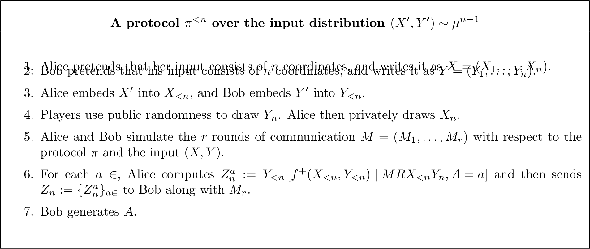
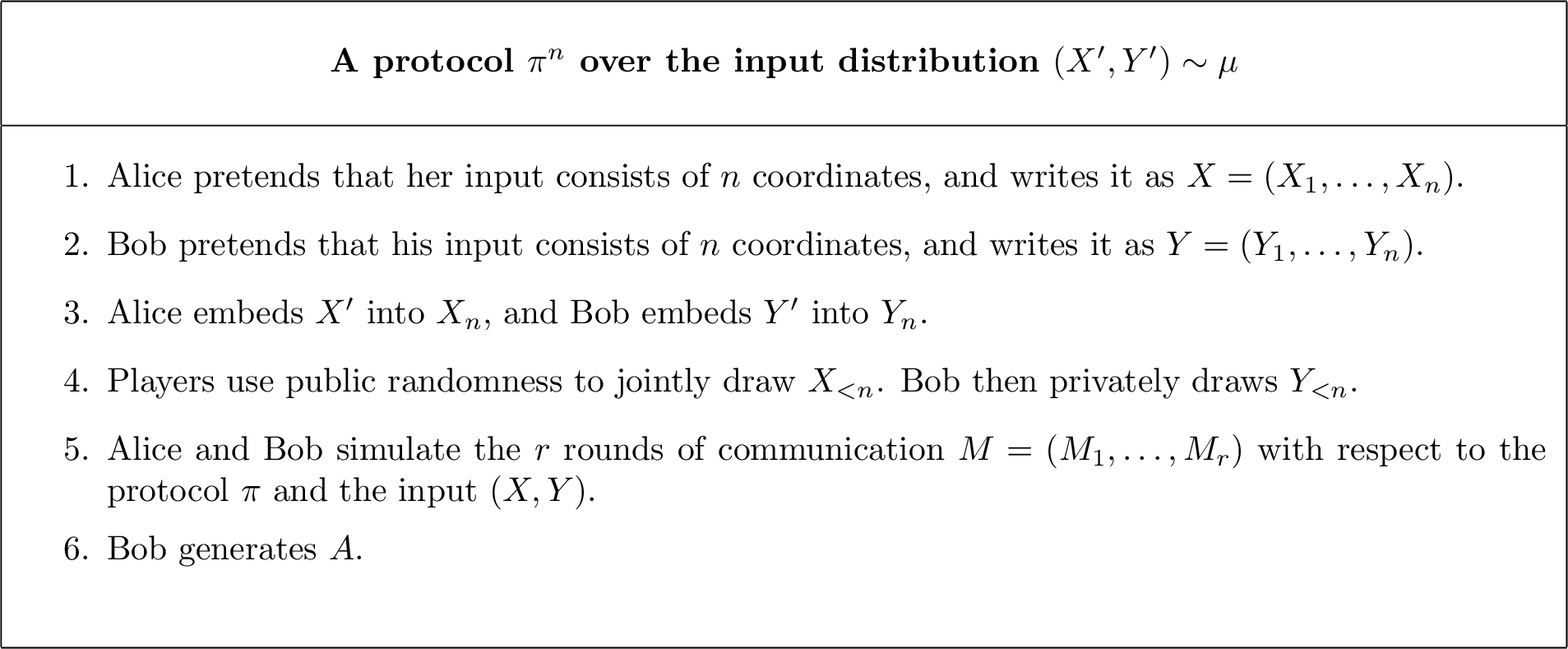
Equivalently, we may adopt the following distributional view of each protocol.

• \(\pi^n = (X_n, Y_n, M, A, RX_{<n})\).

• \(\pi^{<n} = (X_{<n}, Y_{<n}, M \odot Z_n, A, RY_{n})\) where \(Z_n\) consists of \(Z_n^a = \underset{Y_{<n}}{\mathbb{E}} \left[f^+(X_{<n}, Y_{<n}) \mid MRX_{<n}Y_n, A=a\right]\) for each \(a \in \mathcal{A}\) computable solely by Alice. Here we write \(M \odot Z_n\) to denote the \(r\)-round transcript \(M\) with Alice appending \(Z_n\) to her last message \(M_r\). Note further that for a fixed value of \(a\in \mathcal{A}\), \(Z^a_n\) is a deterministic function of \(MRX_0Y_1\).

For convenience, we make the same assumption as in the previous section: each \(Z_n^{a}\) takes values from a discrete set \(\mathcal{Z}\). As before, we will lift this assumption shortly.

5.0.0.2 Decomposition of Information Costs.

Analogous to the proof of 7, without the \(Z_n\) in \(\pi^{<n}\), the information costs of \(\pi^n\) and \(\pi^{<n}\) sums up to the information cost of \(\pi\). The extra message \(Z_n\) of \(\pi^{<n}\) incurs additional \(O(|\mathcal{A}| \cdot \log{|\mathcal{Z}|})\) bits, as there are \(|\mathcal{A}|\) choices of \(a\), and each \(Z_n^{a}\) can be represented with \(O(\log{|\mathcal{Z}|})\) bits. This yields the following information cost decomposition. We omit its formal proof for brevity.

5.0.0.3 Decomposition of Variances.

Analogous to 11, we show that the decomposition of variance still holds, if the variance of \(\pi^n\) is now evaluated from Bob’s perspective.

5.0.0.4 Lifting the assumptions about \(Z_n\).

We now lift the assumptions of exact communication of \(Z_n\) in the same fashion as we did in 4. For each \(a \in \mathcal{A}\), instead of Alice sending each \(Z_n^a\) exactly, she sends the value of \((Z_n^a)^2\) rounded down to closest multiple of \(\frac{\Delta}{32}\). The implications of such rounding scheme are as follows.

• Observe that the range of each \(Z_n^{a}\) is \([0,n^2]\). This allows us to set a discrete space \(\mathcal{Z}\) to be \(\{0, \frac{\Delta}{32}, \ldots \frac{\Delta}{32}, \ldots, \frac{\Delta}{32} \cdot \lfloor n^2 \cdot \frac{32}{\Delta}\rfloor\}\). As a result, \(|\mathcal{Z}| = O(\frac{n^2}{\Delta})\). Plugging this into 10, the decomposition of information costs may incur an additive loss of \(O(|\mathcal{A}| \cdot \log{\frac{n}{\Delta}})\) bits.

• Similar to before, such rounding scheme introduces an additive loss to observer variance of \(\pi^{<n}\) by \(\frac{\Delta}{32}\). Here, though, Bob’s variace does not suffer any losses. As a result, the decomposition of variances may incur an additive loss of \(\frac{\Delta}{32}\).

In summary, by replacing the exact communication of \(Z_n\) by its squared and rounded version, we obtain the following round-preserving decomposition lemma.

We are now ready to prove the main result of this section.

6 Lower Bound Applications↩︎

Finally, we demonstrate the power of the gap-majority lemma by using it to derive lower bounds for the communication complexity of Gap-Hamming and the streaming complexity of triangle counting. We begin by revisiting a few fundamental communication problems and their information lower bounds. These problems, throughout this section, will serve as the base functions for our gap-majority reduction. The first problem is set-disjointness.

The next problem is indexing. In fact, we will use a slightly non-standard variant of indexing which restricts the support size.

We note that there are many known information-theoretic proofs of these lower bounds; see, for example, the folklore arguments of [46], [47] or the comprehensive textbook by Rao and Yehudayoff [48].

6.1 Gap-Hamming↩︎

Consider the following Gap-Hamming problem in the two-player communication setting.

Since its formal introduction by Indyk and Woodruff [32], Gap-Hamming has quickly become one of the central problems in communication complexity. Due to its “gap” structure, it has served as a key tool for proving lower bounds for a variety of problems, such as streaming frequency moment estimation [36]–[38], [40], sketching complexity of graph cuts [41], testing of boolean function properties [39], to name just a few. Notably, early applications of the Gap-Hamming problem were restricted to the one-way communication in which the optimal lower bound \(\Omega(n)\) was quickly established in the original paper of [32]. It was only in 2012 that Chakrabarti and Regev [33] proved that \(\Omega(n)\) bits of communication are required even for protocols with unbounded rounds. Though their original proof was quite technically involved, a sequence of follow-up works [34], [35] provided significantly simpler proofs. Another set of milestones was achieved by [49]–[51], who obtained the explicit information lower bound: they showed that, under various distributions, any protocol computing \(\mathsf{GH}_n\) must reveal \(\Omega(n)\) bits of information about the players’ inputs.

As briefly discussed earlier, \(\mathsf{GH}_n\) is in fact a special case of the gap-majority composition obtained by taking \(f(x,y) := xy\). Therefore, it is almost mandatory for us to recover its optimal \(\Omega(n)\) lower bound through our gap-majority framework. We remark although the lower bound result is not quantitatively novel, we consider our proof strategy to be the main takeaway message: utilizing the gap-majority lemma as a “black-box” tool, our lower bound proof of \(\mathsf{GH}_n\) is merely a simple and clean reduction from the classical set-disjointness problem.

The rest of this subsection will prove 14. We first describe its hard distribution in which we will prove an information lower bound against.

6.1.0.1 Hard distribution \(\mathcal{D}_{\mathsf{GH}}\) for \(\mathsf{GH}_n\).

Let \(n = 4k^{2}t\) for a sufficiently large constant \(k\). We partition the \(n\) coordinates into \(t\) disjoint blocks of size \(4k^{2}\). For each block \(i \in [t]\), Alice receives \(X_i \in \{\pm 1\}^{4k^{2}}\) and Bob receives \(Y_i \in \{\pm 1\}^{4k^{2}}\), jointly drawn from the following distribution \(\mathcal{D}_{\text{block}}\).

1. Sample \((X'_i, Y'_i) \sim \mathcal{D}_{\mathsf{DISJ}_k}\).

2. The first \(3k^{2}\) coordinates of \(X_i\) and \(Y_i\) are indexed by \([k] \times [3k]\) and constructed as follows. For each \(l \in [k]\):

   • If \(l \in X'_{i}\), set \(X_i(l,j) = -1\) for \(1 \le j \le k\), and \(+1\) otherwise.

   • If \(l \notin X'_{i}\), set \(X_i(l,j) = -1\) for \(k+1 \le j \le 2k\), and \(+1\) otherwise.

   • If \(l \in Y'_{i}\), set \(Y_i(l,j) = -1\) for \(1 \le j \le k\), and \(+1\) otherwise.

   • If \(l \notin Y'_{i}\), set \(Y_i(l,j) = -1\) for \(2k+1 \le j \le 3k\), and \(+1\) otherwise.

3. The next \(k^{2}-k\) coordinates of both \(X_i\) and \(Y_i\) are set to \(+1\).

4. The final \(k\) coordinates of \(X_i\) are set to \(+1\), and the final \(k\) coordinates of \(Y_i\) are set to \(-1\).

We now prove the linear lower bound of gap-hamming.

6.2 Triangle Counting↩︎

Consider the following triangle counting problem in a single-pass streaming setting.

A naive streaming algorithm for triangle counting simply stores the entire graph as the stream progresses, which requires \(\widetilde{O}(m)\) bits of memory. Beyond this trivial approach, a long line of work has culminated in a randomized algorithm that uses \(\widetilde{O}\!\left(\frac{mn}{\varepsilon^2 T}\right)\) space [42]–[44], [52]–[54]. In this section, we show that, up to \(\operatorname{polylog}(n)\) factors, these two upper bounds taken together are in fact optimal even with respect to the dependence on \(\varepsilon\).

Our proof of 15 follows a standard approach by reducing \(\mathsf{TC}\) to a new one-way communication problem \(\mathcal{P}\) (state shortly). We assume the setting of parameters \(m,n,\tau,T\) as stated in 15, and may assume further that \(\varepsilon^2 T \geq n\). Let \(\mathcal{A}\) be a streaming algorithm with space \(S\) and succeeds for \(\mathsf{TC}\) with probability \(0.999\). Our ultimate goal is to show that \(S \geq \Omega\left(\frac{mn}{\varepsilon^2T}\right)\). We note that in our upcoming reduction, we shall construct a graph with \(\Theta(n)\) vertices, \(\Theta(m)\) edges, and \(\Theta(T)\) triangles instead of exactly \(n\) vertices, \(m\) edges and \(T\) triangles. These numbers can then be scaled as needed.

Set \(t = \Theta(1/\varepsilon^{2})\), \(k = \Theta(\sqrt{\frac{mn}{\tau}})\), and \(b = \Theta(\varepsilon^2 \tau/n)\) for suitable leading constants. We also ensure that \(t,k,b \geq 1\) which is possible due to the set-up of our parameters. Consider the following one-way (distributional) communication problem \(\mathcal{P}\) which can be interpreted as a \(\pm 0.01\sqrt{t}\) approximation of \(\mathsf{IND}_{k^2, k^2/10}^{+t}\) over the distribution \(\mathcal{D}_{\mathsf{IND}_{k^2, k^2/10}}^{t}\).

1. Sample \(t\) i.i.d. instances of \(\mathcal{D}_{\mathsf{IND}_{k^2, k^2/10}}\), namely \((S_{i}, \ell_{i})\) for each \(i,j \in [t]\).

2. Alice receives all the \(\{S_{i}\}_{i \in [t]}\) and Bob receives all the \(\{\ell_{i}\}_{i \in [t]}\).

3. Alice sends one message \(M\) to Bob, who then are asked to compute \(\sum_{i \in [t]} \mathsf{IND}_{k^2, k^2/10}(S_{i}, \ell_{i})\) within \(\pm 0.01\sqrt{t}\) error.

We will first prove the lower bound of \(\mathcal{P}\) via our round-preserving gap-majority lemma taken with \(r=1\).

We now make the reduction by constructing a one-way protocol \(\pi\) for \(\mathcal{P}\) that succeeds with probability \(0.99\). To do so, the players use their input to construct a graph \(G\) of \(\Theta(n)\) vertices, \(\Theta(m)\) edges, and \(\Theta(T)\) triangles, and then invoke the streaming algorithm \(\mathcal{A}\) for \(\mathsf{TC}\).

6.2.0.1 Vertices.

\(G\) has \(n+2tkb = \Theta(n)\) vertices where the first \(n\) vertices are labeled \(z_{1},...,z_{n}\), and the remaining \(2tkb\) vertices are split into \(2t\) disjoint blocks of size \(kb\) named \(X_{1},\ldots,X_{t}\) and \(Y_{1},\ldots,Y_{t}\). Each block \(X_i\) and \(Y_i\) is further split into \(b\) mini-blocks of size \(k\) named \(X_{i,1},\ldots,X_{i,b}\), and \(Y_{i,1},\ldots,Y_{i,b}\) respectively. There are no edges within the \(X\)’s parts nor within the \(Y\)’s parts.

6.2.0.2 Edges and edge-partition.

For each \(i \in [t]\), consider the input pair \((S_{i}, \ell_{i}) \in \{\pm 1\}^{k^2} \times [k^2]\) given to Alice and Bob respectively. For each \(j \in [b]\), Alice views the induced subgraph \(X_{i,j} \cup Y_{i,j}\) as a vector of dimension \(k^2\). She then encodes \(S_{i} \in \{\pm 1\}^{k^2}\) by drawing the \(k^2/10\) edges corresponding to the positions of 1s. For a pair of vertices \(x \in X_{i,j}\) and \(y \in Y_{i,j}\) that \((x,y)\) encodes \(\ell_{i}\), Bob draws \((z_q,x)\) and \((z_q,y)\) for every \(q \in [n]\). Note that the graph contains \(2nbt + (k^2/10) \cdot bt = \Theta(m)\) edges.

6.2.0.3 Protocol \(\pi\).

Alice starts the streaming algorithm \(\mathcal{A}\) with an empty graph. She then inserts all of her edges and send the memory content to Bob. Bob then continues inserting all of his edges. In the end, Bob queries \(\mathcal{A}\) for \(\widetilde{T}\) such that \(|T-\widetilde{T}| \leq \varepsilon T\) with probability \(0.99\) and answers \(\frac{2\widetilde{T}}{bn}-t\).

6.2.0.4 Wrapping-up.

By chaining 16 and 17, \(\pi\) must use \(\Omega\left(\frac{mn}{\varepsilon^2T}\right)\) bits of communication. Since the sole message from Alice is the memory content of \(\mathcal{A}\) which is \(S\) bits, we have \(S \geq \Omega\left(\frac{mn}{\varepsilon^2T}\right)\) as desired.

7 Acknowledgement↩︎

The authors thank Elena Gribelyuk, Cheng Jiang, Yang Hu, Yinchen Liu, and Santhoshini Velusamy for helpful discussions that inspired this work. We are especially grateful to and credit Sepehr Assadi for pointing out the potential application of gap-majority lemmas to streaming triangle counting in 6.2. We also thank anonymous FOCS 2026 reviewers for their valuable feedback and for identifying typographical errors in an earlier draft.

AI Disclosure. Numerical calculations in the proof of [lem:gapmaj95then95low95variance] (shown in Appendix 8) were assisted by ChatGPT.

8 Proof of [lem:gapmaj95then95low95variance]↩︎

We give the missing proof of [lem:gapmaj95then95low95variance], which closely follows Claim 6 of [45].

References↩︎

---

1. Department of Computer Science, Princeton University. Supported by NSF CAREER award CCF-233994.  [ps3122@princeton.edu](ps3122@princeton.edu){.uri}↩︎

2. Department of Computer Science, Princeton University. Supported by NSF CAREER award CCF-233994.  [yuhch123@gmail.com](yuhch123@gmail.com){.uri}↩︎

3. We will formally define the information cost in 2.↩︎

4. To see this, consider the protocol \(\eta\) from Alice’s perspective. Knowing \(x\), her prior view of \(y\) is equally likely to be \(x-1\) or \(x+1\). After the communication, she gains a small constant advantage in predicting \(y\). Hence, her posterior view of \(y\) shifts from her prior view by \(\Omega(1)\), meaning that she must have learned \(\Omega(1)\) bits of information.↩︎

5. In fact, there are other known lower bounds parameterized by additional structural parameters. We omit these bounds since our regime is parameterized solely by \(n,m,T\), and \(\varepsilon\). Readers may consult [44] for further references.↩︎