ArgTca: Attribute Relation Graph for
Test-Time Calibration of Vision-Language Models
July 08, 2026
Abstract
Reliable confidence estimation remains a key limitation of test-time adaptation in vision–language models (VLMs), where prompt tuning improves zero-shot accuracy but often degrades calibration due to entropy-driven overconfidence. Prior approaches mitigate this using LLM-derived class attributes and contrastive regularization, yet treat attributes independently, ignoring their relational structure. We propose ArgTca, which represents (class, attribute) pairs as nodes in a Symbolic Attribute Graph and trains a Graph Attention Network (GAT) via contrastive objectives to produce structurally informed embeddings capturing inter-attribute dependencies.
We introduce two attribute selection strategies: ArgTca-Div for intra-class diversity and ArgTca-Disc for inter-class discrimination. Experiments across \(9\) benchmarks show that ArgTca-Div reduces average ECE(\(\downarrow\)) by \(\sim37\%\) over baselines, whereas ArgTca-Disc consistently performs as the second-best variant, reducing average ECE by \(\sim17\%\) over baselines. These results suggest that modeling symbolic attribute interactions provides a principled approach for reliable test-time adaptation in VLMs.
1 Introduction↩︎
Vision-language models (VLMs) such as CLIP [1] have shown strong zero-shot image recognition by aligning images and text in a shared embedding space through large-scale contrastive pretraining. CLIP performs zero-shot classification of an image by computing cosine similarities between its visual embedding and class-conditioned text features generated from prompt templates such as “a photo of a {class}”. While effective, such templates are suboptimal and domain-agnostic. Test-time prompt tuning (TPT) [2] addresses this by optimizing prompt tokens for each test image using only its own augmented views, with no labeled data. However, TPTs entropy minimization objective inherently drives the model toward overconfident predictions, producing miscalibrated outputs, quantified by the Expected Calibration Error (ECE) [3]. It poses a fundamental barrier to deploying VLMs in safety-sensitive applications such as healthcare diagnostics and autonomous systems, where unreliable uncertainty estimates can have serious consequences.
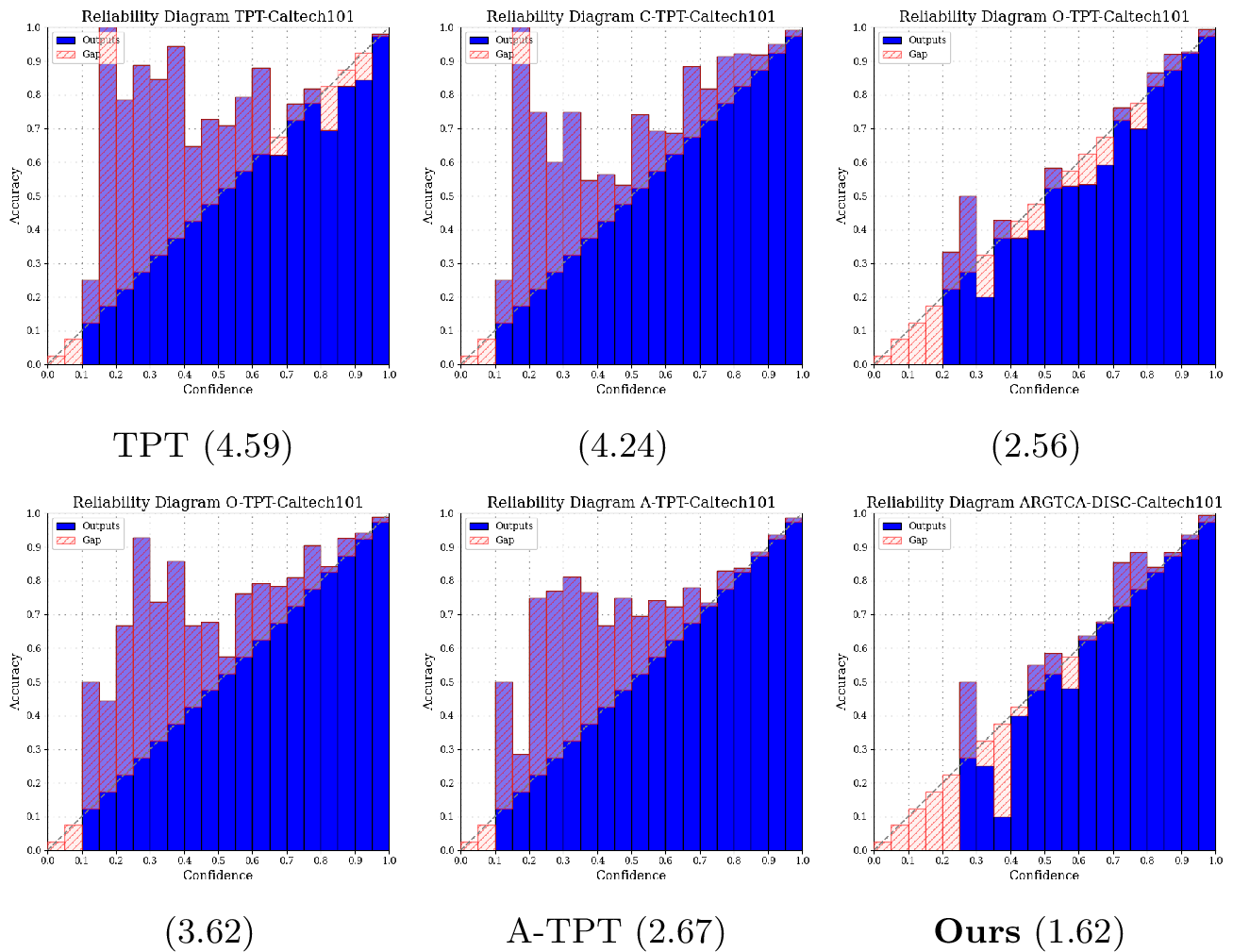
A key insight motivating recent work is that calibration and accuracy are largely decoupled: different prompts can achieve nearly identical top-1 accuracy while exhibiting significantly divergent ECE [4]. This implies that the geometry of the textual feature space, rather than predictive accuracy alone, governs how well-calibrated a VLMs predictions are. C-TPT [4] and O-TPT[5] exploit this by adding a feature-dispersion loss and angular dispersion respectively, that spreads class-conditioned text features across the hypersphere. TCA [6] complements these geometric objectives by adding LLM-extracted visual attributes for semantically grounded prompt initialization, combined with a contrastive intra-class and inter-class regularization over the resulting text embeddings, achieving strong calibration.
1.0.0.1 Structural limitations of TCA.
Despite strong calibration performance, TCA exhibits two structural failures that directly degrade the geometry of class-conditioned text features. First, attributes are selected as a flat set based on cosine-similarity without any relational context: on texture-rich datasets such as DTD, attributes such as rough, bumpy, and grainy are nearly collinear in CLIP’s embedding space, so top-\(M'\) selection clusters attribute embeddings tightly and undermines the separation that calibration requires. Second, attributes shared ubiquitously across different classes—such as mammal across leopard, dolphin, and beaver in Caltech101—carry diminished discriminative capacity, leaving their embeddings proximate across class boundaries. Both the failure modes are invisible to TCA’s selection procedure, which operates purely on similarity based ordering of LLM generated attributes without any notion of relational geometry between attributes.
We propose ArgTca (Attribute Relation Graph for Test-time Calibration Adaptation), a graph-based framework that addresses both structural failures through a Symbolic Attribute Graph (SAG) constructed by representing (class, attribute) pairs as nodes, trained offline via a Graph Attention Network with no task supervision. Two selection strategies derived from the graph — ArgTca-Div for intra-class diversity and ArgTca-Disc for inter-class discrimination. Both strategies operate at zero additional test-time cost — Note: the graph is trained once offline and selection is performed before tuning begins.
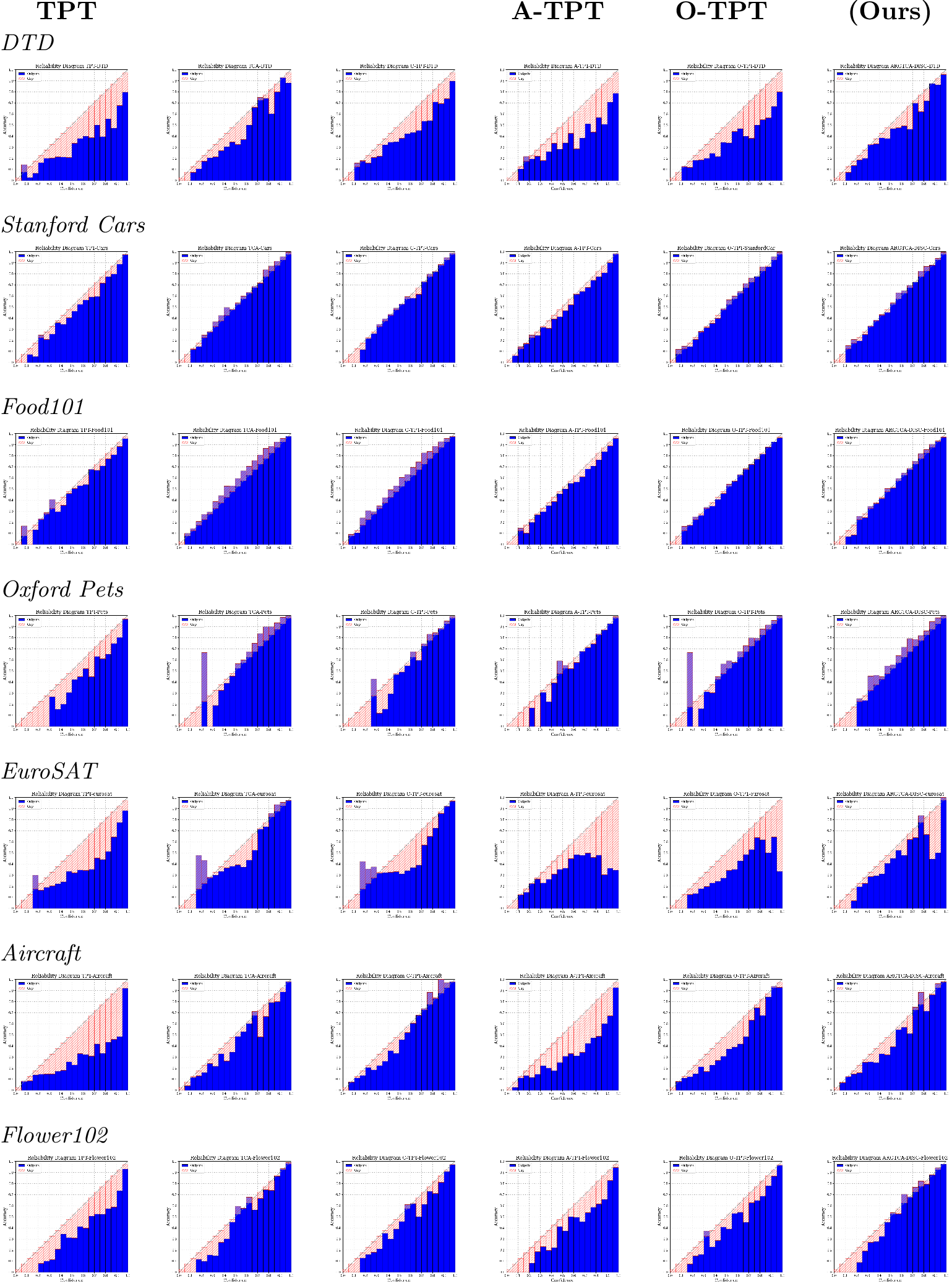
We validate ArgTca across nine benchmark datasets spanning fine-grained recognition, texture classification, and domain-shifted imagery and demonstrate empirically that graph-structured relational reasoning over attributes is a key driver of calibration improvement — as shown in Figure 1, ArgTca produces reliability diagrams most closely aligned with the perfect calibration diagonal, outperforming existing prompt-tuning baselines. Our key contributions are:
We identify two structural failures in TCA: near-synonymous intra-class attributes that cluster on the hypersphere, and ubiquitous cross-class attributes that carry no discriminative capacity yet receive no suppression. We construct a Symbolic Attribute Graph (SAG) from class specific attributes and train a Graph Attention Network via supervised contrastive learning to produce relational embeddings capturing intra-class complementarity and cross-class redundancy.
We introduce two selection strategies from graph-refined embeddings: ArgTca-Div, maximising intra-class semantic complementarity; and ArgTca-Disc, maximising distance from all other-class embeddings. Both strategies operate at zero additional test-time cost and are evaluated across nine benchmarks using CLIP ViT-B/16.
2 Related Work↩︎
2.1 Test-Time Adaptation of VLMs↩︎
Foundation models such as CLIP [1], [7] enable zero-shot classification by aligning image and text in a shared embedding space. While learned prompt methods like CoOp [8] and CoCoOp [9] improve over hard prompts, they require labeled data, limiting zero-shot applicability. TPT [2] removes this constraint by adapting prompts via entropy minimization over augmented views of a single test image, extended further by DiffTPT [10] and PromptAlign [11] through improved augmentation and distribution alignment. However, entropy minimization drives overconfident predictions across all TPT-family methods, significantly degrading calibration relative to the zero-shot baseline[4].
2.2 Calibration of Vision-Language Models↩︎
Post-hoc methods such as temperature scaling [3] and Platt scaling [12] require labeled validation data, making them impractical at test time. C-TPT [4] establishes that TPT degrades calibration, and that well-calibrated prompts exhibit higher Average Text Feature Dispersion (ATFD). O-TPT [5] refines this, showing that ATFD displaces the feature centroid without ensuring pairwise angular separation — the operative quantity for calibration on the unit hypersphere. A-TPT [13] addresses a further degeneracy in O-TPT when \(N > |D|\) (\(N\): #datapoints, \(D\): feature dimensions), enforcing pairwise angular separation without dimensional constraints. TCA [6] initializes prompts with LLM-extracted visual attributes and applies intra- and inter-class contrastive regularization, but treats attributes as a flat set ignoring relationships — a gap our work addresses.
2.3 Graph-Based VLM Adaptation↩︎
GNNs [14], [15] have proven effective for learning over relational data. In VLM adaptation, GraphAdapter [16] uses dual knowledge graphs for supervised few-shot transfer, HGCLIP [17] encodes label taxonomies for hierarchical classification, and VCGPrompt [18] builds visual concept graphs for prompt learning. These works demonstrate that relational structure over the label space improves representation quality in VLMs, however are designed to operate in supervised settings, not for zero-shot calibration. In contrast, ArgTca utilizes symbolic graph edges in a fully label-free setting, specifically targeting calibration improvement.
ArgTca occupies the intersection of all three research threads retaining TCA’s semantically grounded prompt initialization, corrects its flat-set attribute selection through a Symbolic Attribute Graph, and directly optimizes the geometric properties of text feature space that govern calibration — none of the prior works simultaneously achieves.
3 Methodology↩︎
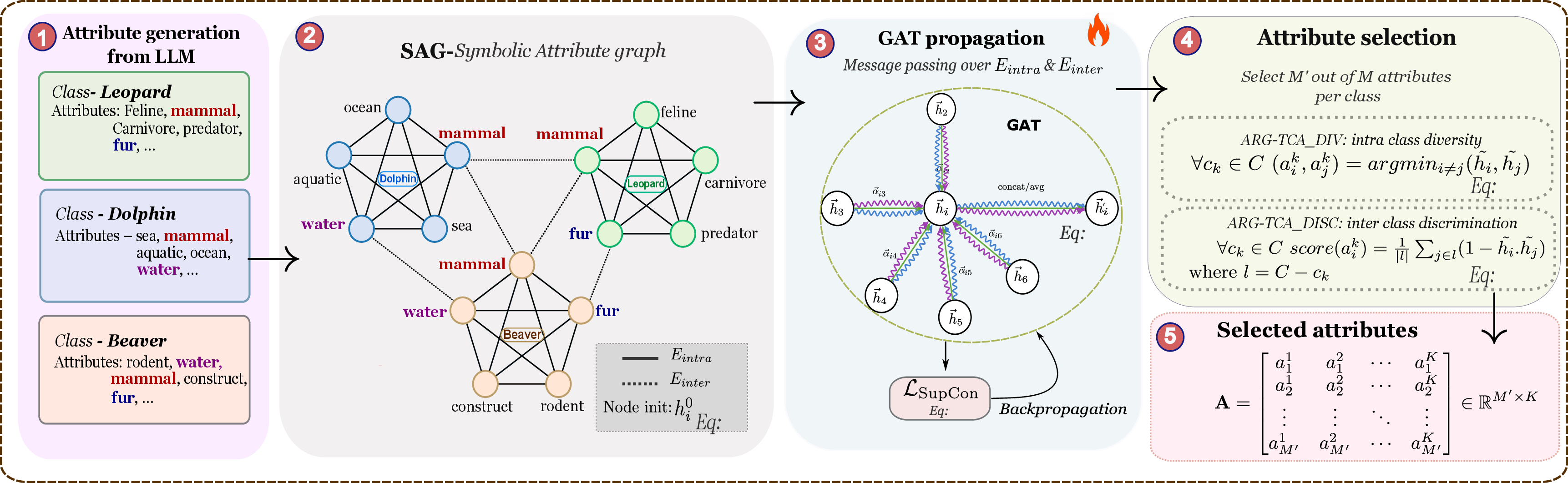
ArgTca replaces TCA’s [6] similarity-based attribute selection with
a graph-informed selection via two phases. In Phase 1, a Symbolic Attribute Graph (SAG) is constructed over all \((\text{class, attribute})\) pairs, with intra-class edges (\(E_{\text{intra}}\)) encoding within-class attribute relations and inter-class edges (\(E_{\text{inter}}\)) encoding cross-class sharing. A Graph Attention Network (GAT) is trained with a
supervised contrastive objective (Eq. 7 ), producing relational embeddings that capture intra-class complementarity and inter-class redundancy. These drive two principled selection strategies: ArgTca-Div, which selects the most semantically complementary attribute pair per class, spanning the widest semantic range for diverse prompt adaptation signals; and ArgTca-Disc, which scores each
attribute by its mean angular distance from all other-class nodes and selects the top-\(M'\) per class — these maximally class-specific descriptors strengthen TCA’s inter-class
regularizer. Figure 2 gives an overview of the proposed graph-informed attribute selection.
In Phase 2, selected attributes initialize the standard TCA test-time tuning procedure without modification. The graph’s contribution is purely structural: deciding which attributes appear, not how they
are represented. Moreover, graph training and attribute selection are performed once offline before testing, incurring no additional test-time cost.
3.1 Preliminaries↩︎
3.1.0.1 Notation
Let \({C} = \{c_1,\ldots,c_K\}\) be a set of \(K\) class labels and \(A_k = \{a_1,\ldots,a_M\}\) be the set of \(M\) LLM-generated visual attributes for class \(k\), giving \(N = K \times M\) total (\(c_k,a_j\)) pairs. A full list of notations is provided in Table 4 in Appendix.
3.1.0.2 TCA background
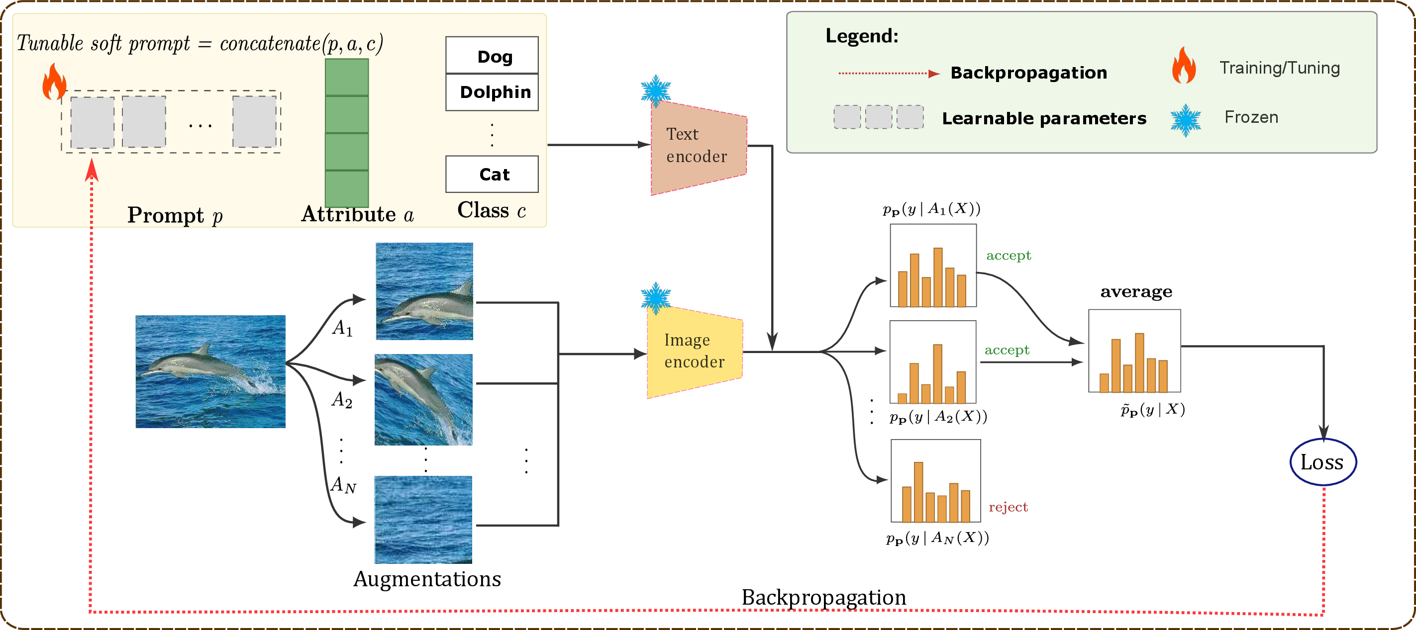
TCA [6] initializes soft prompts using visual attributes and defines per-class text features via
attribute-conditioned prompt embeddings. For each class \(k\) and each of its \(M'\) selected attributes, a prompt is assembled as \[t_{k,m} = \mathbf{p} \oplus \mathbf{a}_m \oplus \mathbf{c}_k, \label{eq:prompt}\tag{1}\] where \(\mathbf{p}\) is the learnable soft context (initialised to "a photo of a"),
and \(\mathbf{a}_m\), \(\mathbf{c}_k\) are the token embeddings of the attribute and class name strings, respectively. The text feature is \(f_{k,m} =
g(t_{k,m})\), where \(g(\cdot)\) denotes the frozen CLIP text encoder. Class probabilities combine all attribute prompts via a bag-of-attributes softmax aggregation:
\[\small p(y = k \mid x) = \frac{\displaystyle\sum_{m=1}^{M'} \exp\!\bigl( f_{\mathrm{img}}(x)\cdot f_{k,m}/\tau\bigr)}{\displaystyle\sum_{k'=1}^{K}\sum_{m=1}^{M'} \exp\!\bigl( f_{\mathrm{img}}(x)\cdot f_{k',m}/\tau\bigr)} \label{eq:tca95prob}\tag{2}\] where \(\tau\) is CLIP’s learned logit scale. The test-time objective minimizes: \[\mathcal{L}_{\mathrm{TCA}} = \mathcal{L}_{\mathrm{TPT}} - \alpha\,\mathcal{L}_{\mathrm{inter}} + \beta\,\mathcal{L}_{\mathrm{intra}} \label{eq:tca95loss}\tag{3}\] with \(\alpha\) weights how aggressively class centroids \(\mu_k\) are pushed away from the global centroid \(\mu\), and \(\beta\) weights how tightly each class’s attribute embeddings \(f_{k,m}\) are pulled toward their class centroid \(\mu_k\). \(\mathcal{L}_{\mathrm{TPT}}\) is the entropy of the average prediction over the \(\lfloor B \cdot p_{\mathrm{sel}}\rfloor\) most confident of \(B\) augmented views. \(\mathcal{L}_{\mathrm{inter}} = \frac{1}{K}\sum_k\left\lVert\mu_k - \mu\right\rVert_2\) is the mean distance of class centroids \(\mu_k = \frac{1}{M'}\sum_m f_{k,m}\) from the global centroid \(\mu\); maximizing it spreads classes apart. \(\mathcal{L}_{\mathrm{intra}} = \frac{1}{K}\sum_k\frac{1}{M'}\sum_m\left\lVert f_{k,m}-\mu_k\right\rVert_2\) is minimized to make each class’s attribute prompts consistent. Only \(\mathbf{p}\) is updated; all other parameters are frozen.
3.2 Phase 1 — Symbolic Attribute Graph and GAT Training↩︎
3.2.1 Node Initialization↩︎
We adopt the \(M\) visual attributes per class provided by [6], generated offline via GPT-4
prompting across all nine benchmark datasets. Specifically, for each class \(c_k\), an LLM is prompted with the class name to produce a list of descriptive visual attributes \(a_m\), which are subsequently ranked in descending order of relevance by cosine similarity between the attribute and class name embeddings [6]. Each class-attribute pair (\(c_k\), \(a_j\)) is represented as a graph node, initialized with \(\ell_2\)-normalized EOS hidden state obtained by encoding the phrase “a \(a_{j}\) of a \(c_k\)” through frozen CLIP text encoder,\(g(\cdot)\): \[\mathbf{h}^{(0)}_i \;=\; g\!\left(\texttt{"a } a_j \texttt{ of a } c_k\texttt{"}\right)
\;\in\; \mathbb{R}^{d} \label{eq:h0}\tag{4}\]
3.2.2 Symbolic Attribute Graph (Sag)↩︎
We define the edge set \(E\) via a symbolic rule over the node vocabulary: \[\mathcal{E}= \Bigl\{(i,j) \Big| i \neq j \text{ and } \underbrace{c_i = c_j}_{{E_{intra}}} \text{ or } \underbrace{a_i = a_j}_{{E_{inter}}}\Bigr\} \label{eq:edges}\tag{5}\]
where both directions are included and self-loops are omitted. In equation 5 \(\mathcal{E}_{\mathrm{intra}}\) connects all attribute nodes belonging to the same class (\(c_i = c_j\)), enabling the GAT to jointly aggregate every attribute perspective of a class; \(\mathcal{E}_{\mathrm{inter}}\) connects nodes that sharing a common attribute token across different classes — for instance, mammal links leopard, dolphin, and beaver in Caltech101 — allowing the GAT to propagate how the same descriptor is contextualized differently across class neighborhoods.
For \(K\) classes each with \(M\) attributes, \(|\mathcal{E}_{\mathrm{intra}}| = K \cdot M \cdot (M - 1)\) is guaranteed regardless of the data distribution.
3.2.3 GAT & hybrid Objective↩︎
We use GAT to propagate feature information across \(\mathcal{E}_\text{intra}\) and \(\mathcal{E}_\text{inter}\) edges so that each attribute node aggregates both the complementary perspectives of its own class and the cross-class context of any shared attribute, producing node embeddings \(\mathbf{h}^{(L)}\) where same-class attributes are pulled into a compact, coherent cluster while cross-class attribute representations are pushed apart. Concretely, at layer \(l\), the updated embedding of node \(i\) is computed as: \[\mathbf{h}^{\text{l}}_i = ELU \left(\Big\|_{h=1}^{H} \sum_{j \in \mathcal{N}(i)} \alpha^h_{j} \cdot \mathbf{W}_h \mathbf{h}_j^{l-1}\right) \label{eq:gat}\tag{6}\] where \(\|\) denotes head-wise concatenation over \(H\) attention heads, \(\mathcal{N}(i)\) is the set of neighbors of node \(i\) under \(\mathcal{E}\), and \(\mathbf{W}^{(l)}_h \in \mathbb{R}^{d/H \times d}\) is the head-specific linear projection at layer \(l\). The attention coefficient \(\alpha^{(l,h)}_{ji}\) measures the relative importance of neighbor \(j\) to node \(i\) under head \(h\), and \(ELU\) induces non-linearity. Full architectural details including the attention coefficient computation are given in section 8 of appendix.
GAT Training Objective The GAT is trained using supervised contrastive loss [19] where same-class \((c_k, a_j)\) nodes form positives, and all inter-class nodes form negatives.
\[\small \mathcal{L}_\text{SupCon} = \frac{1}{|\mathcal{A}|}\sum_{i \in \mathcal{A}} \frac{-1}{|P(i)|} \sum_{p \in P(i)} \\ \log \frac{\exp\left(\tilde{\mathbf{h}}_i^{\top} \cdot \tilde{\mathbf{h}}_p / \tau\right)}{\displaystyle\sum_{j \neq i} \exp\left(\tilde{\mathbf{h}}_i^{\top} \cdot \tilde{\mathbf{h}}_j / \tau\right)} \label{eq:supcon}\tag{7}\] where \(\tilde{\mathbf{h}}^{(L)} = \mathbf{h}^{(L)}/ \|\mathbf{h}^{(L)}\|_2\) and \(\mathcal{A}\) = nodes that have at least one positive. This trains the GAT to produce class-cohesive representations in \(\mathbf{h}^{(L)}\) space while discriminating against all other classes.
3.3 Attribute Selection (Post training)↩︎
After GAT training, the learned \(\mathbf{h}^{(L)}\) is used to select \(M'\) of the \(M\) attributes per class using one of two criteria. Both strategies operate entirely offline at zero test-time cost.
3.3.0.1 ArgTca-Div — Intra-class diversity
For each class \(c_k\in C\), select the pair \((a_i^k, a_j^k)\) with the minimum cosine similarity in the graph-refined embedding space — i.e., the most semantically complementary pair: \[(a_i^k, a_j^k) = \arg\min_{i \neq j \in I_k}\; \tilde{h}^{(L)}_i \cdot \tilde{h}^{(L)}_j. \label{eq:div}\tag{8}\]
3.3.0.2 ArgTca-Disc:
For each node \(a_i^k\) in class \(c_k\), we compute discriminability score measuring its mean angular distance from all other-class nodes:
\[\text{score}(a_i^k) \;=\; \frac{1}{|\bar{\Omega}_k|} \sum_{j \notin \Omega_k} \Bigl(1 - \cos\!\bigl(\tilde{h}^{(L)}_i,\;\tilde{h}^{(L)}_j\bigr)\Bigr), \label{eq:disc}\tag{9}\] where \(\Omega_k\) denotes the global node indices for class \(k\) and \(\bar{\Omega}_k\) all other-class indices. The top \(M'\) attributes by score are selected per class.
3.4 Phase 2 — Test-Time Tuning↩︎
3.4.0.1 Prompt construction
For each \(c_k\) and its \(M'\) attributes selected in Phase 1, prompts are assembled via Eq. 1 , with \(\mathbf{a}_m\) and \(\mathbf{c}_k\) as frozen CLIP token embeddings. The per-class text feature is \(f_{k,m} = g(t_{k,m})\) and class probabilities follow Eq. 2 . The full positional breakdown is given in Table ¿tbl:tab:prompt95breakdown?. \[\small \label{prompt95layout} \text{prompt}\, t_{k,m} = \underbrace{[\mathrm{SOS}]}_{\text{pos }0} \Big\| \underbrace{\mathbf{p}}_{\text{pos }1\text{-}n_\text{ctx}} \Big\| \underbrace{{a}_m^k, \text{cls tokens},\ldots}_{\text{ pos }n_\text{ctx}+1\;\cdots\;76}\tag{10}\]
3.4.0.2 Test-time objective & inference
For each test image, the top \(\lfloor B \cdot p_\text{sel} \rfloor\) most confident of \(B\) augmented views are selected and a single AdamW step minimizes \(\mathcal{L}_{\text{TCA}}\) (Eq. 3 ) on \(\mathbf{p}\). Final prediction uses the non-augmented image with the updated \(\mathbf{p}\), which is reset before each new test image. Figure 7 in appendix illustrates the prompt-tuning process.
4 Experimental Setup↩︎
4.1 Datasets and Baselines↩︎
We evaluate on nine benchmarks datasets, using ViT-B/16 as CLIP backbone and following the evaluation protocol of baselines [1], [20]. Dataset details are provided in section 7 in appendix. Furthermore, we compare our proposed approach against recent, state-of-the-art approaches:
TCA [6]: The direct predecessor, which initializes prompts with LLM-generated visual attributes and applies contrastive intra- and inter-class regularization. Our method builds on and improves upon TCA’s attribute selection procedure.
C-TPT [4]: Adds a text feature dispersion loss (ATFD) to TPT [2] to improve calibration.
O-TPT [5]: Replaces ATFD with pairwise angular separation between class centroids.
A-TPT [13]: Fixes O-TPT’s degeneracy when classes exceed embedding dimension.
All baselines are re-evaluated under identical hyperparameters tuned on the Caltech101 validation set, following the protocol of TCA ([6]).
4.2 Implementation Details↩︎
All experiments are done on a single A100 80GB GPU. The CLIP backbone is fully frozen throughout both phases.
4.2.0.1 Phase 1 — Offline Graph Training.
Each dataset’s attribute graph is constructed from \(N_{\text{attr}} = 10\) LLM-generated attributes per class (from [6]), giving \(K \times 10\) graph nodes. The Graph Attention Network (AttributeGAT; 2 layers, 4 heads, 512-dimensional node features) is trained for 100 epochs with supervised contrastive loss (Eq. 7 ), temperature \(\tau = 0.07\), and the Adam optimizer with learning rate \(10^{-3}\). Phase-1 training is done offline and completes in under two minutes per dataset.
4.2.0.2 Phase 2 — Test-Time Prompt Tuning.
We follow the standard TCA evaluation protocol: soft context initialised to “a photo of a” (\(n_{\text{ctx}} = 4\)), 64 augmented views per test image with the top 10% selected by entropy, and a single gradient step per image with batch size 64. Regularization weights: ViT-B/16 uses \(\alpha = 10\), \(\beta = 35\); \(M'{=}2\) attributes per class are selected from the graph-refined embeddings via either the diversity (ArgTca-Div) or discriminability (ArgTca-Disc) criterion.
4.2.0.3 Metrics
We report top-1 accuracy (Acc, %, \(\uparrow\)) and Expected Calibration Error (ECE, %, \(\downarrow\)) computed with 20 equal-width bins following [6]. Lower ECE indicates better-calibrated predictions.
5 Results↩︎
5.1 Main Results↩︎

Table 1 shows that ArgTca-Div achieves the best average ECE of \(4.45\%\), reducing miscalibration by \(26.7\%\), \(31.5\%\), \(42.4\%\), and \(48.0\%\) over C-TPT, TCA, O-TPT, and A-TPT respectively, while improving average accuracy simultaneously. ArgTca-Disc achieves the highest average accuracy of \(64.68\%\), with an ECE of \(5.90\%\) — a \(2.8\%\), \(9.2\%\), \(23.7\%\), and \(31.0\%\) reduction over C-TPT, TCA, O-TPT, and A-TPT respectively. Notably, A-TPT achieves competitive accuracy (\(64.84\%\)) but at a significantly higher calibration cost (ECE: \(8.55\%\)). ArgTca-Disc breaks this trade-off — matching A-TPT’s accuracy within \(0.2\%\) while reducing its ECE by \(31\%\), confirming that graph-structured attribute reasoning provides consistent calibration gains.
| Method | |||||||||||
|---|---|---|---|---|---|---|---|---|---|---|---|
| Pre-trained Backbone: CLIP Vit-B/16 | Embedding dimension: 1024-d | |||||||||||
| TPT (NeurIPS’22) | Acc. | 93.83 | 87.08 | 66.32 | 69.31 | 84.70 | 23.61 | 46.70 | 42.79 | 67.27 | 64.62 |
| ECE | 4.59 | 5.77 | 5.25 | 13.27 | 4.05 | 16.48 | 21.35 | 21.49 | 13.01 | 11.70 | |
| C-TPT (ICLR’24) | Acc. | 93.35 | 84.14 | 65.45 | 69.79 | 83.28 | 23.85 | 46.04 | 27.8 | 59.7 | 61.49 |
| ECE | 4.24 | 2.77 | 1.94 | 5.21 | 3.77 | 12.27 | 15.16 | 3.89 | 6.07 | ||
| (ECML’25) | Acc. | 93.82 | 90.51 | 65.92 | 69.18 | 69.18 | 24.96 | 44.73 | 45.52 | 66.9 | 63.31 |
| ECE | 2.56 | 6.3 | 7.85 | 3.67 | 5.28 | 4.52 | 11.26 | 5.25 | 6.50 | ||
| O-TPT (CVPR’25) | Acc. | 93.67 | 88.55 | 65.65 | 69.96 | 83.52 | 23.46 | 46.87 | 42.85 | 66.90 | 64.60 |
| ECE | 3.62 | 7.15 | 3.13 | 7.75 | 19.75 | 20.92 | 3.56 | 7.73 | |||
| A-TPT (ICLR’26) | Acc. | 93.75 | 88.49 | 66.44 | 69.83 | 83.57 | 23.34 | 47.22 | 43.29 | 67.64 | 64.84 |
| ECE | 2.67 | 10.38 | 2.20 | 13.64 | 19.81 | 17.53 | 6.11 | 8.55 | |||
| (Ours) | Acc. | 92.82 | 89.48 | 65.07 | 70.36 | 83.64 | 24.69 | 47.34 | 32.84 | 69.63 | 63.99 |
| ECE | 3.44 | 2.75 | 4.83 | ||||||||
| (ours) | Acc. | 93.19 | 88.91 | 66.47 | 69.59 | 83.85 | 25.05 | 46.63 | 39.53 | 68.70 | 64.68 |
| ECE | 3.37 | 4.29 | 19.81 | ||||||||
5.2 Calibration Quality: Confidence Distributions and Reliability↩︎
The confidence bin plots (Figure 4) reveal that TCA, O-TPT, and A-TPT accumulate incorrect (red) predictions at high confidence levels, indicating systematic overconfidence. ArgTca-Disc achieves the lowest ECE of \(1.62\%\) at \(93.2\%\) accuracy, with incorrect predictions concentrated at low confidence and correct predictions (green) dominating the high-confidence region. By contrast, O-TPT (ECE: \(3.61\%\)) and TCA (ECE: \(2.56\%\)) exhibit red-green mixing in mid-confidence bins (2–4), while A-TPT (ECE: \(2.67\%\)) partially improves but still misclassifies samples at low confidence.
The radar plot (Figure 3) confirms this trend across all nine benchmarks: ArgTca consistently occupies the innermost region, with gains most pronounced on Aircraft (ECE: \(1.21\%\) vs.\(8.19\%\) for A-TPT), Food101 (\(1.75\%\) vs.\(2.02\%\) for A-TPT), and Flower (\(2.88\%\) vs.\(10.38\%\) for A-TPT). Reliability diagrams (Figures 1, 8) further corroborate this, with ArgTca showing the closest alignment to the calibration diagonal — particularly in high-confidence bins (0.8–1.0) — confirming that graph-based attribute selection suppresses overconfidence without inducing underconfidence.
5.3 Accuracy–Calibration Trade-off↩︎
The two selection strategies encode complementary objectives. ArgTca-Div selects the most semantically complementary attribute pair per class, maximizing angular spread in \(\mathbf{h}^{(L)}\) space. The resulting diverse prompt initialization provides strong gradient signals for both \(\mathcal{L}_{\mathrm{intra}}\) and \(\mathcal{L}_{\mathrm{inter}}\), driving higher accuracy alongside well-calibrated text distributions. ArgTca-Disc instead targets attributes maximally distant from other-class embeddings, initializing prompts with high inter-class separation and more conservative updates — effective on datasets with severe inter-class confusion (e.g., Caltech101, Aircraft) but less consistent across all nine benchmarks.
Recommendation: ArgTca-Div for broad cross-dataset calibration; ArgTca-Disc when inter-class confusion dominates.


Figure 4: Confidence bin plots on Caltech101 (ViT-B/16). Green/red indicate correct/incorrect predictions. ArgTca-Disc achieves the lowest ECE with the cleanest separation between correct and incorrect predictions across confidence bins.. a — TCA, b — O-TPT, c — A-TPT, d — ArgTca (Ours)
5.4 Ablation Studies↩︎
| Variant | Sel. | Caltech101 | OxfordPets | DTD | |||
|---|---|---|---|---|---|---|---|
| 3-4(lr)5-6(lr)7-8 | Acc | ECE | Acc | ECE | Acc | ECE | |
| (Full) | Div | 92.82 | 2.52 | 89.48 | 47.34 | ||
| Disc | 93.19 | 88.91 | 46.63 | 6.36 | |||
| Div | 93.18 | 2.36 | 89.32 | 3.84 | 45.04 | ||
| Disc | 93.51 | 90.00 | 3.50 | 45.74 | 5.31 | ||
| Div | 92.21 | 2.73 | 88.74 | 3.87 | 46.81 | 5.65 | |
| Disc | 93.39 | 2.60 | 88.99 | 3.71 | 45.98 | 8.95 | |
| Div | 93.10 | 2.53 | 88.63 | 3.44 | 45.92 | 5.16 | |
| Disc | 92.25 | 2.43 | 88.50 | 3.55 | 44.27 | 6.33 | |
4pt
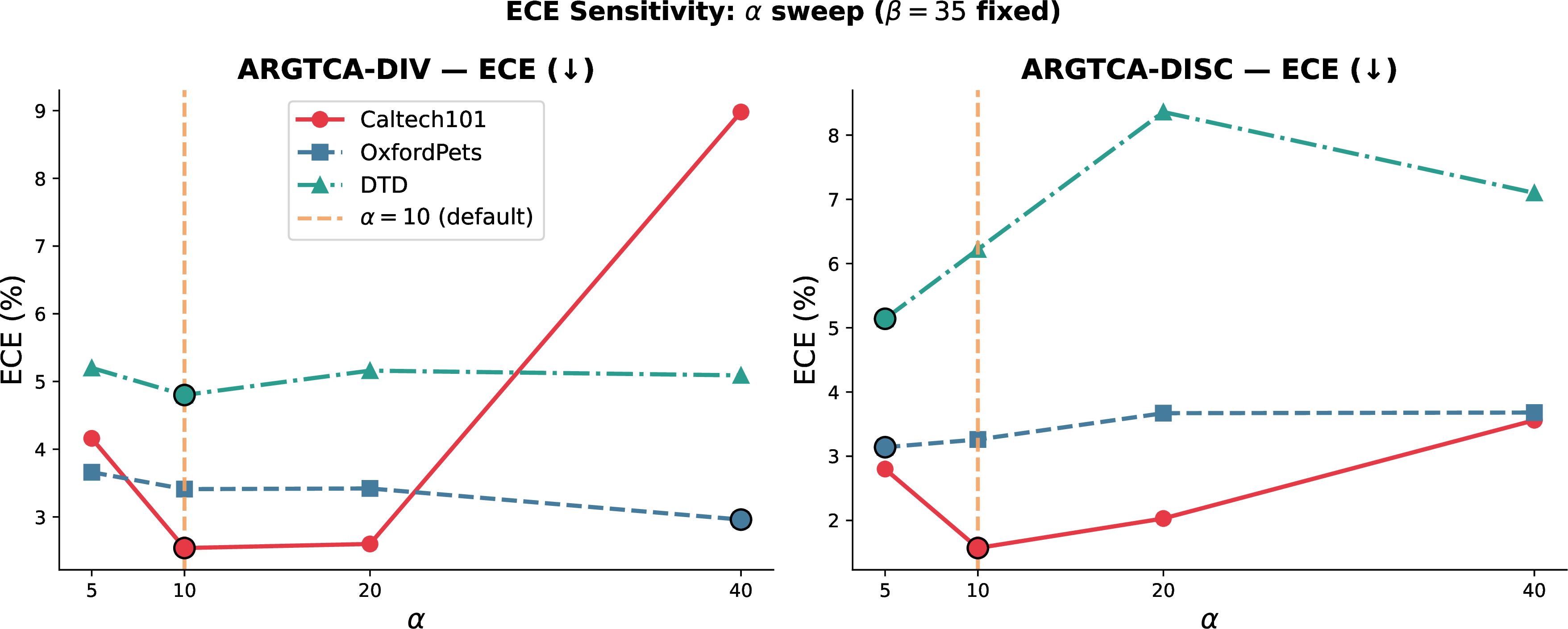
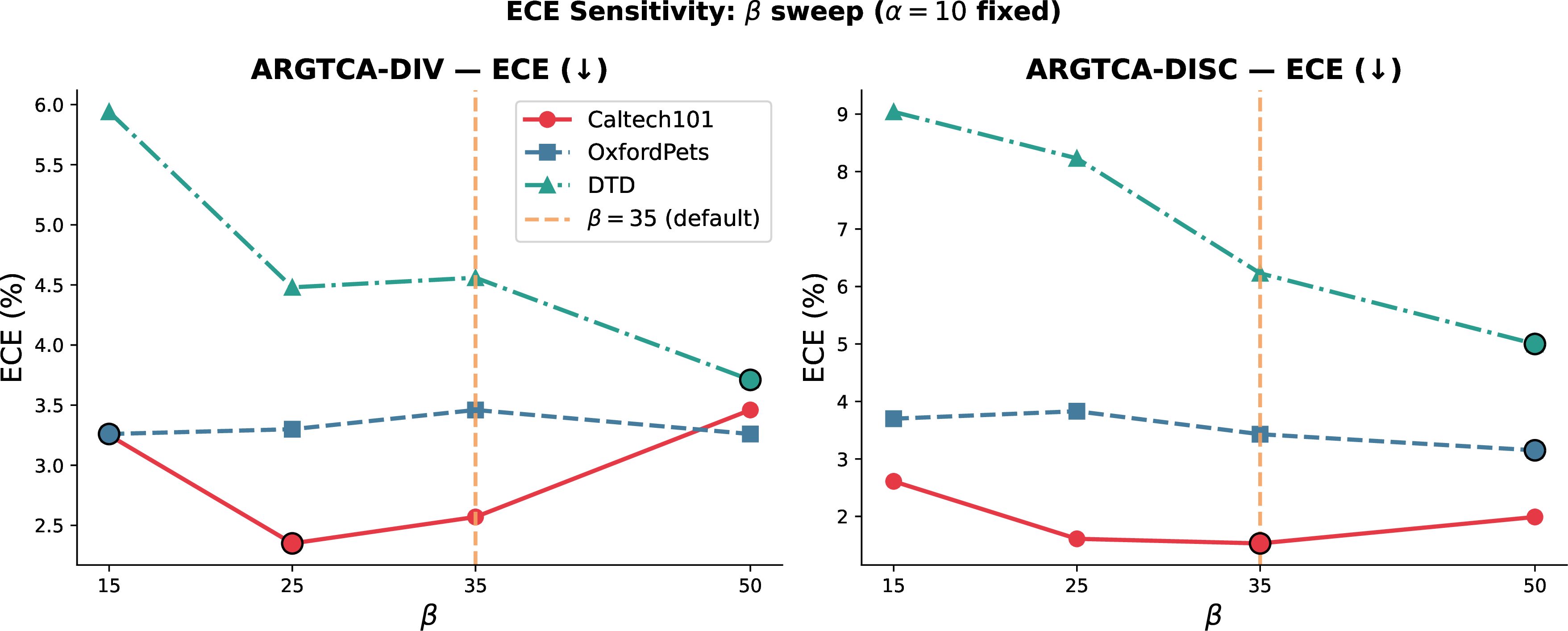
All ablations use ViT-B/16 on Caltech101, OxfordPets, and DTD. We ablate three components of ArgTca: (i) edge structure — Sag trained with \(\mathcal{E}{=}\emptyset\), removing message passing while retaining contrastive training and Div/Disc selection; (ii) GAT training — Div/Disc applied directly to raw CLIP EOS embeddings \(\mathbf{h}^{(0)}\), skipping Phase 1 entirely; and (iii) selection criterion — Phase 1 run in full but with random attribute selection (\(M'{=}2\), seed 42). We additionally sweep \(\alpha \in \{5,10,20,40\}\) (\(\beta{=}35\) fixed) and \(\beta \in \{15,25,35,50\}\) (\(\alpha{=}10\) fixed). A detailed per-ablation description and hyperparameter sweep figures are in shown Appendix 9.
The ablation results (Table 2) confirm the contribution of each component. Removing edge structure (i) degrades ECE on DTD for both Div (\(3.17{\to}4.91\)) and Disc (\(6.36{\to}4.91\)). Skipping GAT training entirely (ii) causes the largest degradation: DTD ECE rises to \(5.65\) (Div) and \(8.95\) (Disc), confirming that relational contrastive training is critical for texture-heavy datasets. Random selection (iii) degrades DTD Div ECE from \(3.17\) to \(5.16\) with minimal accuracy impact, directly isolating the geometric Div/Disc criteria as the operative calibration mechanism.
| Dataset | Class | (top-2) | ||
|---|---|---|---|---|
| Caltech101 | ||||
| airplane | aircraft, travel | transportation, altitude | jet, airline | |
| camera | image, digital | digital, vintage | dslr, digital | |
| chair | design, chair | design, director’s | elegant, chair | |
| face | images, human | natural, adults | emotion, casual | |
| motorbike | motorbike, pillion | seat, suspension | suspension, motorbike | |
| OxfordPets | ||||
| Abyssinian | Abyssinian, cats | restful, observant | cats, feline | |
| Boxer | Dog, Boxer | Athletic, Friendly | Boxer, Pet | |
| Maine Coon | Feline, Cat | Tabby, Fluffy | Kitten, Coon | |
| Persian | Adorable, Persian | Adorable, Lying | Persian, Adorable | |
| Shiba Inu | Shiba, Dog | Cute, Foxy | Inu, Shiba | |
| DTD | ||||
| banded | design, casual | material, colorful | casual, colorful | |
| bumpy | uneven, unequal | unequal, geometric | knobby, indented | |
| crystalline | natural, crystals | natural, glittering | shimmering, crystals | |
| dotted | variation, design | variation, fashion | dots, stylized | |
| woven | interwoven, craftsmanship | material, organic | handwoven, craftsmanship | |
4pt
5.4.0.1 Attributes selected by TCA vs.ArgTca.
TCA selects top-\(M'\) attributes by cosine similarity to the class name, surfacing near-synonymous descriptors that cluster tightly on the hypersphere. ArgTca-Div selects the maximally complementary pair in \(\mathbf{h}^{(L)}\) space; ArgTca-Disc selects the pair most distant from all other-class embeddings. Per-class examples are in Table 3.
5.4.0.2 Hyperparameter sensitivity (\(\alpha\), \(\beta\)).
Both weights are stable across \(\alpha \in \{5,10,20,40\}\) and \(\beta \in \{15,25,35,50\}\): ECE varies by at most \({\sim}2\%\) across the full sweep, with the ViT-B/16 defaults (\(\alpha{=}10\), \(\beta{=}35\)) lying in the stable plateau (see Figures 5–6). Full ECE sweep for both selection strategies are provided in Appendix 9.
6 Conclusion↩︎
We present ArgTca, a test-time calibration framework for CLIP that replaces flat attribute selection in TCA with graph-relational reasoning. A GAT trained via supervised contrastive loss over the Symbolic Attribute Graph (Sag) produces attribute embeddings encoding intra-class diversity and inter-class discriminability, giving rise to two selection criteria: ArgTca-Div and ArgTca-Disc. Across nine benchmarks, ArgTca-Div achieves the lowest average ECE (\(4.45\) ), reducing miscalibration by up to \(48\%\). Ablations confirm that edge topology, contrastive training, and geometric selection each contribute independently. Future works include a unified selection objective jointly optimiing diversity and discriminability, and cross-dataset graph transfer to remove the per-dataset offline build requirement.
Limitations↩︎
6.0.0.1 LLM attribute quality.
The method inherits TCA’s dependence on LLM-generated attribute quality. Domains where LLMs produce generic or noisy attributes (e.g., satellite imagery) remain challenging. Richer, domain-specific attribute generation strategies may be needed for such cases.
6.0.0.2 Accuracy–calibration tradeoff.
ArgTca-Div and ArgTca-Disc are complementary but not jointly optimal: across benchmarks, ArgTca-Div tends to improve accuracy while ArgTca-Disc tends to reduce ECE, and no single variant dominates on both metrics simultaneously. Practitioners must choose a selection strategy based on deployment priority, which limits plug-and-play usability without prior knowledge of the target domain.
6.0.0.3 Dataset-specific graph.
The Sag and GAT are trained independently per dataset, so applying ArgTca to a new benchmark requires re-running Phase 1. The learned graph structure does not transfer across datasets or domains, and Phase 1 cannot be run when the class vocabulary is unavailable at build time, constraining applicability in fully zero-shot settings.
6pt
@p0.72r@ Section & Page
A Datasets &
B GAT Architecture Details &
Attention and Aggregation &
Residual, Normalisation, and Projection &
Node Attention Score &
C Ablation Studies &
C.1 Attribute Comparison: TCA vs. vs. &
C.2 Zero Graph Edges &
C.3 No GAT Training (Raw CLIP EOS Embeddings) &
C.4 Random Attribute Selection &
C.5 Hyperparameter Sensitivity (\(\alpha\), \(\beta\)) &
D Prompt Token Layout &
E Notation Reference &
TCA Pipeline Overview &
Reliability Diagrams Across All Datasets (ViT-B/16) &
Attribute Comparison: TCA vs. vs. &
Ablation Results &
Prompt Token Layout — &
Notation Reference &
| Position | Content | Notes |
|---|---|---|
| 0 | SOS token embedding | Frozen |
| \(1\)–\(n_{\text{ctx}}\) | Soft prompt \(\mathbf{p} \in \R^{n_{\text{ctx}} \times D_t}\) | Learnable (tuned at test time) |
| \(n_{\text{ctx}}+1\) | \({a}_m^k\) | graph selected attribute |
| \(n_{\text{ctx}}+2\) – \(L\!-\!1\) | Class tokens + EOS + padding | Frozen |
7 Datasets↩︎
We evaluate on nine benchmarks: Caltech101 [21] (general objects), StanfordCars [22], FGVC-Aircraft [23], OxfordPets [24], and Flowers102 [25] (fine-grained recognition), Food101 [26] (food categories), DTD [27] (perceptual textures), UCF101 [28] (action recognition), and EuroSAT [29] (satellite land-use). We follow the standard [8] test splits used in TCA [6], evaluating on the test set only with no labeled data.
Notation Reference↩︎
A full list of all the notations used in the document are provided in Table 4.
| Symbol | Shape / Type | Meaning |
|---|---|---|
| \(K\) | scalar | Number of classes |
| \(M\) | scalar | Attributes loaded per class (num_attributes\(=10\)) |
| \(M'\) | scalar | Attributes selected for injection (prompt_attributes\(=2\)) |
| \(N = K \times M\) | scalar | Total graph nodes |
| \(d = 512\) | scalar | CLIP token embedding dimension |
| \(c_k\) | string | Class name for class \(k\) |
| \(a_j\) | string | \(j\)-th attribute string |
| \((c_k, a_j)\) | tuple | Node \(i\) in the graph |
| \(\hzero_i\) | \(\R^d\) | Initial node embedding (CLIP EOS hidden state) |
| \(\hL_i\) | \(\R^d\) | GAT output (refined node embedding) |
| \(\p\) | \(\R^{n_{\text{ctx}} \times d}\) | Soft prompt context (trainable, Phase 2) |
| \(g(\cdot)\) | \(\R^d\) | CLIP text encoder EOS hidden state |
| \(f(\cdot)\) | \(\R^{d_{\text{out}}}\) | CLIP text encoder full output (after projection \(\mathbf{T}\)) |
| \(\tau\) | scalar | InfoNCE temperature |
| \(\alpha,\,\beta\) | scalars | TCA inter / intra loss weights |
8 GAT Architecture Details↩︎
Our graph-based attribute selection follows the Graph Attention Network (GAT) framework of [15], which assigns learned importance weights to neighborhood edges during message passing, enabling the model to selectively aggregate information from the most relevant neighbors. Our Sag is an undirected graph; each undirected edge \(\{u, v\} \in \mathcal{E}\) is represented as two directed edges \((u \to v)\) and \((v \to u)\) during message passing, following standard practice in GAT implementations.
8.0.0.1 Attention and aggregation.
For each edge \(\{u,v\}\) and head \(h\), the normalized attention coefficient is: \[\small \alpha_{uv,h} = \frac{ \exp\!\left(\mathrm{LeakyReLU}( \mathbf{a}_h^\top[\widetilde{\mathbf{h}}_{u,h} \| \widetilde{\mathbf{h}}_{v,h}])\right) }{ \sum_{u'\in\mathcal{N}(v)} \exp\!\left(\mathrm{LeakyReLU}( \mathbf{a}_h^\top[\widetilde{\mathbf{h}}_{u',h} \| \widetilde{\mathbf{h}}_{v,h}])\right) },\] where \(\widetilde{\mathbf{h}} = \mathbf{h}^{(l)}W_{\text{layer}}\) is the linearly projected embedding. Node representations are updated as: \[\small \widetilde{\mathbf{h}}^{(l)} = \mathrm{ELU}\!\left( \mathrm{concat}_{h=1}^{H} \!\left[\sum_{u\in\mathcal{N}(v)} \mathrm{drop}(\alpha_{uv,h})\cdot\widetilde{\mathbf{h}}_{u,h}\right] \right).\]
8.0.0.2 Residual, normalisation, and projection.
After \(L\) layers, a residual connection (with \(W_{\mathrm{res}}\) initialised to \(\mathbf{I}\)) mitigates over-smoothing, followed by \(\ell_2\) normalisation: \[\mathbf{h}^{(L)} = \mathrm{normalize}\!\left( \widetilde{\mathbf{h}}^{(L)} + W_{\mathrm{res}}\,\mathbf{h}^{(0)} \right).\] A two-layer MLP projects to the final embedding: \(\mathbf{z} = W_2(\mathrm{GELU}(W_1\mathbf{h}^{(L)}+\mathbf{b}_1))\).
8.0.0.3 Node attention score.
A scalar importance score per node, used for attribute selection in ArgTca-Div and ArgTca-Disc, is computed as the mean attention coefficient across heads and layers: \[\mathrm{attn}[v] = \frac{1}{LH} \sum_{l=1}^{L}\sum_{h=1}^{H} \frac{1}{|\mathcal{N}(v)|} \sum_{u\in\mathcal{N}(v)} \alpha_{uv,h}.\] This scalar serves as the basis for attribute selection in both ArgTca-Div and ArgTca-Disc (Section 3.2).
9 Ablation Studies↩︎
9.1 Attribute comparison: TCA vs.ArgTca-Div vs.ArgTca-Disc.↩︎
The table 3 lists the two attributes selected per method for a representative subset of classes from Caltech101, OxfordPets, and DTD. TCA ranks attributes by cosine similarity between each attribute’s frozen CLIP embedding and the class name embedding, selecting the top-\(M'\); ArgTca-Div selects the most complementary pair by minimum pairwise cosine similarity in \(\mathbf{h}^{(L)}\) space; ArgTca-Disc selects the pair with highest mean cosine distance to all other-class embeddings in \(\mathbf{h}^{(L)}\) space.
9.2 Zero graph edges.↩︎
To isolate the contribution of the Sag edge structure, we train the GAT with \(\mathcal{E}= \emptyset\): all nodes are present and trained via supervised contrastive loss, but no message passing occurs. Without edges, each GAT layer reduces to an independent per-node linear transform; no cross-class or within-class structural context propagates. Attribute selection uses the same Div/Disc criteria on these edge-free embeddings. The calibration drop on DTD relative to the full model (Table 2) confirms that the Sag’s edge topology — not the contrastive objective alone — drives selection quality.
9.3 No GAT training (raw CLIP EOS embeddings).↩︎
We skip Phase 1 entirely and apply the Div/Disc selection criteria directly to the initial embeddings \(\mathbf{h}^{(0)}\) (frozen CLIP EOS hidden states, Eq. 4 ), without any contrastive training. This tests whether GAT training adds value beyond the semantic geometry already present in CLIP’s encoder. The DTD ECE degrades substantially (Disc: \(8.95\) vs.\(6.36\) for the full model), showing that contrastive relational training is necessary for reliable attribute discrimination on texture-heavy datasets.
9.4 Random attribute selection.↩︎
We run Phase 1 in full (SAG construction, GAT training) but replace Div/Disc selection with a random draw of \(M' = 2\) attributes per class (seed 42). This isolates the selection criterion: random selection degrades ECE on DTD (Div: \(5.16\) vs.\(3.17\) for the full model) while leaving Caltech accuracy largely unchanged, confirming that the geometric Div/Disc criteria are the operative mechanism for calibration improvement, not merely the graph training.
9.5 Hyperparameter sensitivity (\(\alpha\), \(\beta\)).↩︎
Figures 5 and 6 show ECE as \(\alpha\) and \(\beta\) are swept independently (\(\alpha \in \{5,10,20,40\}\) with \(\beta{=}35\) fixed; \(\beta \in \{15,25,35,50\}\) with \(\alpha{=}10\) fixed), evaluated on Caltech101, OxfordPets, and DTD for both ArgTca-Div and ArgTca-Disc. Both metrics are stable across the swept range: ECE varies by at most \({\sim}1.5\%\) on Caltech101 and \({\sim}2.0\%\) on DTD for \(\alpha\), and by at most \({\sim}1.8\%\) on DTD for \(\beta\). The optimal region is \(\alpha \in [10,20]\) and \(\beta \in [25,35]\); the ViT-B/16 defaults (\(\alpha{=}10\), \(\beta{=}35\)) lie within this plateau, confirming robustness to precise hyperparameter choice.

References↩︎
Equal contribution.↩︎