quantum differential equations ,quantum algorithms ,one-ancilla ,qubit-efficient ,extrapolation ,classical postprocessing ,circuit depth

1 Introduction↩︎

Differential equations are among the most important mathematical models in science and engineering, with wide-ranging applications across many disciplines. Designing quantum algorithms for differential equations has been an important direction in quantum computing. In particular, time-dependent linear differential equations have received significant attention, especially in dissipative and non-unitary regimes where the dynamics cannot be directly treated as standard Hamiltonian simulation. Significant developments in quantum algorithms have been made for this task. While we do not attempt to give an exhaustive survey here, representative state-of-the-art approaches include methods based on quantum linear systems algorithms with history-state encodings [1]–[6], time-marching methods [7], [8], linear combinations of Hamiltonian simulation [9]–[14], unitary-dilation [15]–[18], Lindbladian embeddings [19], quantum eigenvalue processing [20], and other fault-tolerant primitives. We remark that this dissipative regime is a standard setting shared across state-of-the-art quantum algorithmic frameworks for general linear differential equations, rather than an additional assumption specific to the present work or to a particular line of work.

As in many areas of quantum algorithms, existing quantum differential equation solvers can be broadly viewed from two complementary perspectives. On the one hand, near-term algorithms are designed to be more compatible with current or early fault-tolerant hardware, often avoiding expensive coherent control, large ancilla registers, or deep circuit constructions. Variational and other NISQ approaches fall into this category, but rigorous performance guarantees are often difficult to establish in general. On the other hand, fully fault-tolerant quantum algorithms are developed with provable guarantees and can achieve excellent, sometimes optimal and near-optimal asymptotic scaling. However, these algorithms typically rely on advanced fully fault-tolerant primitives such as block-encodings, quantum linear systems algorithms (QLSA), quantum singular value transformation (QSVT), linear-combination-of-unitaries (LCU) techniques, compression gadget, or coherent control over many time steps. These ingredients can require many ancilla qubits and complicated circuit structures, making them less friendly to realize on near-term or early fault-tolerant devices.

A recent algorithm in [21] provides a different point in this landscape. It gives a one-ancilla quantum algorithm for linear differential equations of the dissipative form considered in this work. The algorithm only uses local Hamiltonian simulation and mid-circuit measurements, preserves locality, and avoids advanced fault-tolerant subroutines such as LCU, QSVT, QLSA, or compression gadget. In this sense, it is both near-term friendly and mathematically rigorous: it is simple enough to be implemented with an optimal one-ancilla qubit, yet still comes with a provable error analysis. This makes it an attractive candidate for early demonstrations of quantum algorithms for non-unitary dynamics and differential equations. This favorable hardware structure, however, comes with a tradeoff. The algorithm does not aim to achieve the optimal asymptotic scaling of fully fault-tolerant quantum differential equation solvers. In particular, its circuit depth has an \(\mathcal{O}(1/\epsilon)\) dependence on the target accuracy \(\epsilon\), reflecting the first-order nature of the underlying quantum algorithm.

Quantum resources remain expensive, even in the early fault-tolerant regime. It is therefore important to use classical computation and processing whenever possible to reduce the amount of coherent quantum evolution required. A particularly successful strategy in this direction is to use classical post-processing, and in particular extrapolation-based algorithmic error mitigation, to reduce quantum resources without changing the underlying quantum simulation primitive. Pioneering works in this direction include [22]–[24], which explored this idea for Hamiltonian simulation, including circuit-depth reduction for Trotter product formulas and qDRIFT, as well as recent works on open quantum systems governed by Lindbladian dynamics [25], [26]. The step-size extrapolation viewpoint is also closely related to zero-noise extrapolation in quantum error mitigation, where data obtained at several effective noise strengths are classically extrapolated to the zero-noise limit [27]–[30].

In this work, we bring this perspective to the one-ancilla quantum algorithm for linear differential equations. The dynamics considered here are not necessarily unitary or completely positive and trace-preserving, as in Hamiltonian or Lindbladian cases. We ask whether extrapolation-based classical post-processing can provably reduce the circuit depth of this near-term-friendly differential equation solver, without changing the underlying quantum circuit or introducing additional ancilla qubits. We answer this question affirmatively for unnormalized observable estimation. For each time step size, we run the one-ancilla circuit to the final time and estimate an unnormalized observable from raw measurement data. We then combine the estimates from multiple step sizes using either Richardson extrapolation or Chebyshev interpolation, thereby extrapolating the observable to the zero-step-size limit. In this way, tools from classical numerical analysis and approximation theory are used to extract a more accurate observable estimate from a family of coarse, hardware-friendly quantum circuits.

Technically, there are two important differences between the present setting and the previously studied Hamiltonian and Lindblad settings. The first difference concerns the regularity estimates for the step-size-dependent observable map, the crucial step for this kind of postprocessing analysis. In Hamiltonian simulation, observable dynamics can be described naturally in the Heisenberg picture by unitary conjugation. In a trace-preserving Lindblad simulation, there is likewise a natural dual semigroup acting on observables. These structures allow one to analyze the step-size dependence of observables directly. In the present postselected ODE setting, however, the successful evolution is described by a non-unitary map acting on state vectors, and the target observable has the form of a quadratic expression involving both the forward map and its Hilbert-space adjoint. When the one-step map is analytically continued to a complex step size, taking the Hilbert-space adjoint becomes anti-holomorphic rather than holomorphic. To obtain derivative bounds for extrapolation, we therefore introduce a holomorphic adjoint lift, which agrees with the usual adjoint on real step sizes but remains holomorphic in the complexified step-size variable. This is the key analytic ingredient that allows us to prove the regularity estimates needed for Richardson extrapolation and Chebyshev interpolation.

The second difference concerns the sampling and observable-estimation model. In Hamiltonian and trace-preserving Lindblad simulation, the simulated object is itself a normalized quantum state or density matrix, and each circuit execution contributes a bounded observable sample from that object. For general non-unitary differential equations, by contrast, a successful quantum output is a normalized state that encodes the solution rather than the unnormalized solution itself, while the squared norm of the unnormalized solution is encoded in the postselection success probability. In the present postselected ODE algorithm, each raw circuit execution includes mid-circuit postselection measurements as part of its built-in design; if one of these measurements returns an undesired outcome, the trajectory is rejected by the postselection procedure. In the original state-preparation view, such rejected trajectories are discarded by design. For unnormalized observable estimation, however, we retain the statistical contribution of these rejection events by recording them as zero-valued samples, while postselection-accepted trajectories contribute the measured observable outcome. This zero-on-rejection estimator is unbiased for the unnormalized observable associated with the time-discretized solution. Consequently, the success probability is automatically incorporated into the raw estimator, and no separate estimation or extrapolation of the success probability is required.

Our main contribution is a complete extrapolation framework for this setting, which reduces the maximum quantum circuit depth from an \(\mathcal{O}(1/\epsilon)\) dependence on the target accuracy \(\epsilon\) to an \(\mathcal{O}(\mathop{\mathrm{polylog}}(1/\epsilon))\) dependence (4, 5). We prove derivative estimates for the unnormalized observable as a function of the time step size (1), establish deterministic bias bounds for general linear post-processing (2), and then specialize the framework to Richardson extrapolation and Chebyshev interpolation, deriving for each the sample complexity, circuit depth, and gate count (4, 5). We also give an upper bound on the sample complexity of the zero-on-failure estimator via concentration inequalities (3), together with a matching lower bound for the independent-shot sampling model (6), showing the resource count to be optimal. Under a geometrically local assumption on the generator, these bounds specialize to an explicit maximum circuit depth in terms of the system size and evolution time (2), and to fully explicit gate count scalings (4, 5). In particular, for Chebyshev interpolation, the maximum circuit depth has only logarithmic-squared dependence on the target accuracy for observable estimation, replacing the inverse-accuracy dependence of the direct first-order method; Richardson extrapolation achieves an even smaller logarithmic dependence (2). However, Richardson extrapolation’s weights grow polynomially in \(1/\epsilon\), rather than Chebyshev’s polylogarithmic growth (3). In geometrically local settings, this gives a depth reduction while preserving the one-ancilla and locality-preserving structure of the original algorithm. We also discuss numerical tests that illustrate the theory. One class of examples comes from convection-diffusion equations, where the differential operator naturally decomposes into anti-self-adjoint and dissipative parts and where the jump operators are simple in either the grid basis or the Fourier basis. Another class comes from the interacting Hatano-Nelson model, a non-Hermitian many-body system exhibiting the non-Hermitian skin effect. These examples demonstrate how the extrapolation framework can be applied both to PDE-inspired problems and to many-body non-Hermitian dynamics.

The rest of the paper is organized as follows. In 2, we review the one-ancilla quantum differential equation solver and present the hybrid quantum-classical extrapolation algorithm. 3 proves the local error bounds, the backward-error derivative estimates, and the deterministic extrapolation error bounds. In 4, we analyze the sampling concentration and quantum resource requirements. 5 presents numerical experiments for convection-diffusion equations and the interacting Hatano-Nelson model. We conclude in 6.

2 Algorithm Overview and Classical Postprocessing↩︎

This section sets up the algorithmic framework used throughout the paper. We first recall the one-ancilla quantum differential equation solver, describe how to classically post-process the measurement outcomes, and then provide a pseudocode for the algorithm.

2.1 Algorithm↩︎

Throughout, we work in a finite dimension and consider the autonomous dissipative linear ODE \[\frac{d}{dt}\ket{\psi(t)}=A\ket{\psi(t)},\quad A=-iH-\sum_{j=1}^{J}D_j, \quad D_j=L_j^\dagger L_j\succeq 0,\] with Hermitian \(H=H^\dagger\) and \(J\) dissipative terms. The exact solution is \(\ket{\psi(t)}=e^{tA}\ket{\psi(0)}\). We assume \(\ket{\psi_0}=\ket{\psi(0)}\) is a normalized initial state, \(\|\ket{\psi_0}\|=1\).

We recall the one-ancilla algorithm construction of  [21], establishing notation for the rest of the paper. For each dissipative term \(D_j\), define the Hermitian dilation \[G_j=\begin{pmatrix} 0 & L_j^\dagger \\ L_j & 0 \end{pmatrix}.\] Post-selecting the ancilla on outcome \(\ket{0}\) after evolving under \(G_j\) for time \(\sqrt{2s}\) gives the system-only operator \[C_j(s) := (\bra{0} \otimes I) e^{i\sqrt{2s}G_j}(\ket{0}\otimes I)=I-sD_j+O(s^2),\] and the leading order term reproduces the dissipative contraction \(e^{-sD_j}\). The closed form of this postselected block is \(C_j(s)=\cos(\sqrt{2s}D_j^{1/2})\), which is proved in 1. Composing the \(J\) postselected blocks with one Hamiltonian simulation step approximates the evolution \(e^{sA}\) over a single time step of size \(s\): \[K_s:=e^{-isH}C_J(s)\cdots C_1(s).\] For a realizable step size \(s=T/R\), \(R\in\mathbb{N}\), the successful state after \(R\) steps is \[\ket{u_s(T)}:=K_s^R\ket{\psi_0},\] with a success probability \(p(s):=\|\ket{u_s(T)}\|^2\). As \(s\rightarrow 0\), \(\ket{u_s(T)}\) approximates \(\ket{\psi(T)}\).

For an observable \(O=O^\dagger\), we aim to estimate the observable signal \[g_O(0):= \bra{\psi(T)}O\ket{\psi(T)}=\bra{\psi_0}(e^{TA})^{\dagger}O(e^{TA})\ket{\psi_0}.\] The data produced by a single circuit run with a step size \(s\) is \[g_O(s):= \bra{u_s(T)}O\ket{u_s(T)},\] and the extrapolation algorithm uses \(g_O(s_\ell)\) for several distinct step sizes \(s_\ell\) to estimate \(g_O(0)\). If the desired target is instead the observable’s value conditional on successful postselection, one could either extrapolate \(f_O(s)=\frac{g_O(s)}{p(s)}\) directly from successful postselections, or extrapolate \(g_O(s)\) and \(p(s)\) separately and then take a ratio.

2.2 The Extrapolation Method↩︎

3.1 shows that achieving accuracy \(\epsilon\) directly, by shrinking the step size \(s\) until the algorithm’s own discretization error is small enough, forces a circuit depth scaling as \(\mathcal{O}(1/\epsilon)\). The rest of this paper shows that this cost can be reduced to \(\mathcal{O}(\mathrm{polylog}(1/\epsilon))\) by running the circuit at several step sizes that remain coarse, and combining the results through classical post-processing.

For a fixed step size \(s\), the circuit is run repeatedly. Each run returns the random variable \[Y_s:=\begin{cases} \text{the measured value of O on the successful branch}, &\text{if every postselection succeeds}\\ 0, &\text{otherwise} \end{cases},\] recording zero rather than discarding the run when a postselection fails, so that \(\mathbb{E}[Y_s]=g_O(s)\) (9). Averaging \(Y_s\) over many repetitions gives an estimate of \(g_O(s)\). 4.1 bounds the number of repetitions needed for a target accuracy.

Running this procedure at several distinct step sizes \(s_1,\ldots, s_m\), each one realizable and each coarser than direct estimation at the target accuracy would require, gives a sequence of estimates of \(g_O(s_1),\ldots, g_O(s_m)\). These are combined into a single estimate of \(g_O(0)\) using a weighted average \(\sum_\ell a_\ell g_O(s_\ell)\), with weights chosen so that the combination agrees with \(g_O(0)\) up to an error controlled by how smoothly \(g_O\) depends on \(s\).

Richardson extrapolation and Chebyshev interpolation, treated in 4.3 and 4.4, are two choices of step sizes and weights for this same procedure. Richardson extrapolation places step sizes at harmonically shrinking values, while Chebyshev interpolation clusters them according to the roots of Chebyshev polynomials. The two trade off differently: Richardson achieves a smaller maximum circuit depth for a given accuracy target, while Chebyshev’s weights are better conditioned, which affects the number of circuit repetitions needed rather than the depth itself.

2.3 Pseudocode↩︎

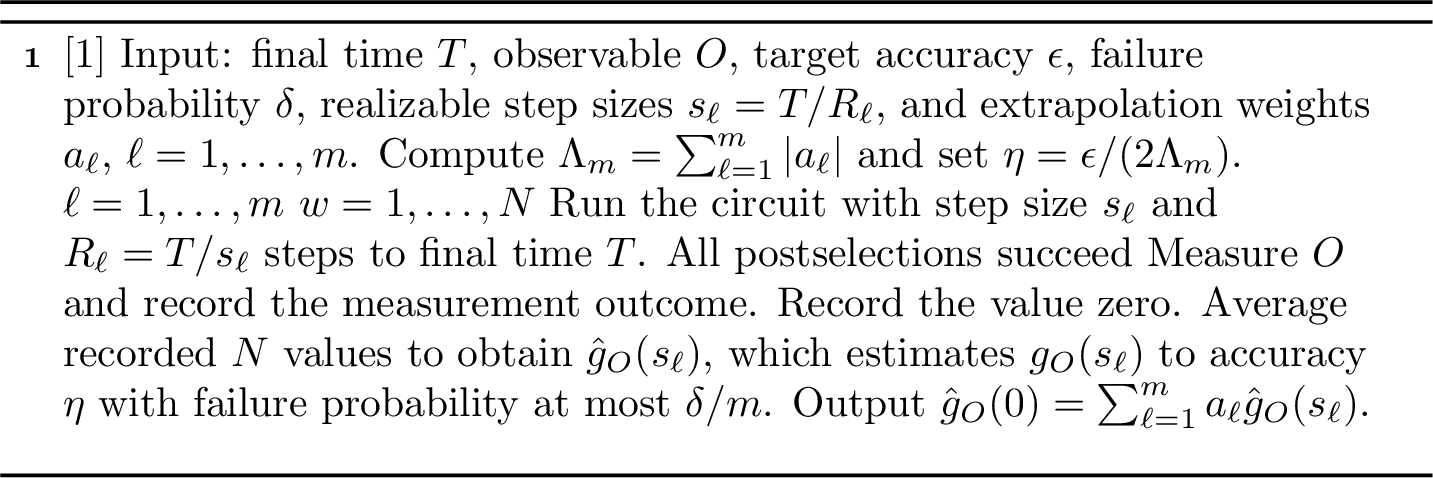
The quantum sampling routine is the same for Richardson and Chebyshev post-processing. The only input that changes is the list of nodes and weights \(\{(s_\ell,a_\ell)\}_{\ell=1}^{m}\). The pseudocode for the algorithm is shown in 1.

3 Numerical Analysis↩︎

This section proves the analytic estimates underlying the postprocessing procedure. We begin with local error bounds for the one-ancilla solver, and then use holomorphic adjoint arguments to obtain derivative estimates for the step-size-dependent observable map. These derivative estimates are the key ingredient in the extrapolation analysis and lead to the deterministic extrapolation bias bounds.

3.1 Local Error Bounds↩︎

We bound the one-step defect \(K_s-e^{sA}\) and its accumulation over \(R\) steps to the final time \(T\). Write \[B_0:=-iH,\quad B_j=-D_j\;\text{for}\; 1\le j\le J, \quad A=\sum_{\nu=0}^{J}B_{\nu},\] and define \[S:=\sum_{\nu=0}^{J}\|B_\nu\|=\|H\|+\sum_{j=1}^{J}\|D_j\|,\] \[\Gamma_{\mathrm{PF}}:=\sum_{0\le \mu<\nu\le J}\|[B_\nu,B_\mu]\|, \quad \Gamma_{\mathrm{cos}}:=\frac{2}{3}\sum_{j=1}^{J}\|D_j^2\|, \quad \Gamma_{\mathrm{loc}}:=\frac{1}{2}\Gamma_{\mathrm{PF}}+\Gamma_{\mathrm{cos}}.\] \(S\) measures the overall strength of the generator. The two error scales have different origins: \(\Gamma_{\mathrm{PF}}\) comes from the noncommutativity of \(J+1\) pieces \(B_\nu\), while \(\Gamma_{\mathrm{cos}}\) is the truncation error of each postselected cosine block. \(\Gamma_{\mathrm{loc}}\) combines them into the single scale used in the bounds below.

Before using these constants, we record a closed-form expression for \(C_j(s)\) that the remainder of this subsection relies on.

This closed form allows us to read off the operator norm of \(C_j(s)\) directly from the spectrum of \(D_j\).

Since \(C_j(s)\) and \(e^{-sD_j}\) are both contractions, we next bound the distance between them directly.

Combined with the contraction bounds above, this per-block defect yields a bound on the error of the full one-step map \(K_s\) against \(e^{sA}\).

Having controlled the error of a single step, we accumulate it over \(R\) repetitions to reach the final time \(T\).

Achieving accuracy \(\epsilon\) therefore requires step size \(s=\mathcal{O}(\epsilon/(T\Gamma_{\mathrm{loc}}))\), or equivalently \(R=\mathcal{O}(T^2\Gamma_{\mathrm{loc}}/\epsilon)\) time steps, giving the \(\mathcal{O}(1/\epsilon)\) circuit depth that motivates the extrapolation framework developed in the remainder of the paper.

3.2 Complex Step Error Bounds↩︎

To bound how \(g_O(s)\) varies with step size, we extend \(C_j(s)\) and \(K_s\) to complex step size \(z\) and study the resulting holomorphic objects. This extension is required for the extrapolation bias estimates established later in this section. The constants \(S\) and \(\Gamma_{\mathrm{loc}}\) from 3.1 reappear unchanged. However, contractivity no longer holds off the real axis, so the bounds below grow exponentially in \(|z|\) rather than remaining bounded by one.

For complex \(z\), define \[C_j(z):=\sum_{k=0}^{\infty}\frac{(-1)^k(2z)^k}{(2k)!}D_j^k, \quad K_z:=e^{zB_0}C_J(z)\cdots C_1(z).\] Then \(K_z\) is entire in \(z\), with \(K_z=I+zA+O(z^2)\).

We first bound the defect of each postselected block against the exponential it approximates on the complex domain.

Then, we collect the exponential bounds that replace contractivity for complex step size.

The defect of \(K_z\) against \(e^{zA}\) now follows the same argument as 1, with each contractivity bound replaced by its complex counterpart from the previous lemma.

This defect bound controls \(K_z\) itself. However, extrapolation requires control of the generator. We therefore show that \(K_z\) admits a well-defined logarithm near \(z=0\) and bound the distance of this logarithm from \(A\).

3.3 Holomorphic Adjoint Lift↩︎

The eventual bound on the observable signal requires both \(A_{\mathrm{eff}}(z)\) and an adjoint object to be holomorphic in \(z\) simultaneously. Writing \(A_{\mathrm{eff}}(z)=A+\sum_{k=1}^{\infty}E_kz^k\) for its Taylor expansion about \(z=0\), guaranteed by 7, the operator adjoint \(A^\dagger _{\mathrm{eff}}(z)\) conjugates both the coefficients \(E_k\) and the scalar \(z^k\), giving \[A^\dagger _{\mathrm{eff}}(z) = A^\dagger +\sum_{k\ge 1}E_k^\dagger \bar{z}^k.\] This expression depends on \(\bar{z}\) rather than \(z\), so it is anti-holomorphic, not holomorphic, off the real axis.

To retain holomorphy, we instead conjugate only the operator coefficients, leaving the scalar \(z^k\) untouched, and define the holomorphic adjoint lift \[A_{\mathrm{eff}}^\sharp (z):=A^\dagger +\sum_{k\ge 1}E_k^\dagger z^k.\] For real \(z=s\), \(\bar{s}=s\), so \(A^\sharp_{\mathrm{eff}}(s)=A_{\mathrm{eff}}(s)^\dagger\) exactly. For complex \(z\), \(A^\sharp_{\mathrm{eff}}(z)\) remains holomorphic.

3.4 Sharp Derivative Bounds for the Observable Signal↩︎

The complex step constructions of the previous two subsections yield derivative bounds on \(g_O(s)\) as a function of the real step size \(s\), required by the extrapolation bias bound later. Cauchy’s integral formula converts a bound on a holomorphic function over a disk into a bound on its derivatives at the center of a smaller disk. It remains to show that the relevant holomorphic lift of \(g_O\) is bounded on such a disk.

Define \(Q:=\max\{S,T\Gamma_{\mathrm{loc}}\}\). This constant combines the strength of the generator with the accumulated effect of dissipation over the full evolution time.

A preliminary identity motivates the construction below. By definition, \(K_s=e^{sA_{\mathrm{eff}}(s)}\), so for the realizable step size \(s=T/R\), \[K_s^R=e^{RsA_{\mathrm{eff}}(s)}=e^{TA_{\mathrm{eff}}(s)}.\] Since \(\ket{u_s(T)}=K_s^R\ket{\psi_0}\), this gives \(\ket{u_s(T)}=e^{TA_{\mathrm{eff}}(s)}\ket{\psi_0}\), which means the holomorphic lift constructed below reproduces \(g_O(s)\) precisely at real, realizable step sizes.

3.5 Deterministic Extrapolation Biases↩︎

The derivative bound established in 1 converts directly into a bias bound for any linear combination of \(g_O(s_\ell)\) values, through the classical Lagrange interpolation remainder formula.

Let \(s_1,\ldots, s_m\) be distinct realizable step sizes in \((0,s_{\mathrm{max}}]\). Define the Lagrange basis polynomials and the resulting extrapolation weights to zero \[\label{eq:def95a95l95Lambda95m} \phi_\ell(x):=\prod_{k\ne \ell}\frac{x-s_k}{s_\ell-s_k}, \quad a_\ell:=\phi_\ell(0), \quad \Lambda_m:=\sum_{\ell=1}^{m}|a_\ell|.\tag{5}\] The extrapolated estimator is \[\hat{g}_O(0):=\sum_{\ell=1}^{m}a_\ell\hat{g}_O(s_\ell),\] where \(\hat{g}_O(s_\ell)\) denotes a raw estimator of \(g_O(s_\ell)\) obtained from circuit measurements.

4 Concentration and Quantum Resource Estimate↩︎

This section establishes the quantum resource estimates. We first use concentration inequalities to derive sampling-cost bounds for the zero-on-failure estimator, and then obtain maximum single-run circuit-depth and total gate-count estimates for both Richardson extrapolation and Chebyshev interpolation.

4.1 Sampling Model and Concentration↩︎

2 bounds the deterministic error of extrapolating from exact values \(g_O(s_\ell)\). In practice each \(g_O(s_\ell)\) is itself only available as an estimate from a finite number of circuit executions, using the random variable \(Y_s\) defined in 2.2. We bound the resulting statistical error and the number of executions required to control it.

Boundedness and unbiasedness are the hypotheses required to apply Hoeffding’s inequality, used below to bound the sampling error.

2 and 3 combine into the total error guarantee for the extrapolated estimator.

4.2 Resource Estimate↩︎

3 gives the number of circuit executions \(N\) required for each step size. We convert this into circuit depth and gate count. For a step size \(s_\ell\), one raw circuit execution to the final time \(T\) has depth \[D_{\mathrm{run}}(s_\ell):=\frac{T}{s_\ell}d_{\mathrm{step}},\] where \(d_{\mathrm{step}}\) is the depth of a single time step. If \(g_\mathrm{step}\) is the gate count of one time step and \(g_{\mathrm{meas}}\) is the gate count of the final measurement of \(O\), one raw execution at \(s_{\ell}\) uses \[G_{\mathrm{run}}(s_\ell):= g_{\mathrm{step}}\frac{T}{s_\ell}+g_{\mathrm{meas}}\] gates.

Note that \(D_\mathrm{total}\) is an aggregate depth budget, the sum of circuit depths over all raw executions, not a gate count.

4.3 Richardson Resources↩︎

Richardson extrapolation instantiates 2 and 3 with harmonically spaced step sizes. Let \(s_\mathrm{max}>0\) be a prescribed upper bound on the largest step size, and define \[R_1=\left\lceil\frac{T}{s_\mathrm{max}}\right\rceil, \quad R_\ell=\ell R_1, \quad s_\ell=\frac{T}{R_\ell}, \quad \ell=1,\ldots, m.\] Since \(R_\ell\in\mathbb{N}\), all of the step sizes are realizable. Moreover, \[s_\ell=\frac{s_1}{\ell}, \quad s_1=\frac{T}{\lceil T/s_{\mathrm{max}} \rceil},\] so the realizable nodes retain the harmonic spacing exactly. We assume throughout that \(s_\mathrm{max}\le T\). Then, \[\frac{s_\mathrm{max}}{2}\le s_1\le s_\mathrm{max}.\] The upper bound is given by the construction. From \(\frac{T}{s_\mathrm{max}} \ge \frac{1}{2}\left\lceil\frac{T}{s_\mathrm{max}}\right\rceil\), we get the lower bound \(s_1=\frac{T}{\lceil T/s_\mathrm{max}\rceil}\ge \frac{s_\mathrm{max}}{2}\).

The product bound controls the deterministic bias, and the two reciprocal bounds control the maximum depth, the aggregate depth, and gate budgets.

4.4 Chebyshev Resources↩︎

Chebyshev interpolation instantiates the same two results with nodes clustered according to Chebyshev polynomial roots rather than spaced harmonically. Let \(s_\mathrm{max}>0\), and suppose the nodes are realizable, \(s_\ell=T/R_\ell\) for some \(R_\ell\in\mathbb{N}\), and satisfy \[c_{ch}\theta_\ell \le s_\ell\le \theta_\ell, \quad \theta_\ell:=s_\mathrm{max}\cos^2\left(\frac{(2\ell-1)\pi}{4m}\right), \quad \ell=1,\ldots, m,\] for a universal constant \(c_{ch}\in(0,1]\).

The reciprocal sum agrees with Richardson’s order in \(m\). The maximum reciprocal does not, since the smallest Chebyshev node decreases quadratically in \(m\) rather than linearly, yielding a different scaling for the maximum depth.

4.5 Geometrically Local Scaling↩︎

Assume \(H\) and each \(L_j\) are geometrically local on \(n\) qubits. Each acts on \(\mathcal{O}(1)\) qubits arranged on a constant dimensional lattice, \(J=\mathcal{O}(n)\), all local coefficients are \(\mathcal{O}(1)\), and each local term fails to commute with at most \(\mathcal{O}(1)\) other local terms.

In a single-ancilla sequential implementation, one time step applies the \(\mathcal{O}(n)\) Hamiltonian terms and the \(J=\mathcal{O}(n)\) dissipative blocks one at a time, each requiring \(\mathcal{O}(1)\) depth and gates by geometric locality, so \(d_\mathrm{step}=\mathcal{O}(n)\) and \(g_\mathrm{step}=\mathcal{O}(n)\). If \(O\) is \(k\)-local, \(g_\mathrm{meas}=\mathcal{O}(k)\).

If \(T\Gamma_\mathrm{loc}\ge S\), then \(Q=T\Gamma_\mathrm{loc}=\mathcal{O}(nT)\).

The remaining quantities, \(N\), \(D_\mathrm{total}\), and \(G_\mathrm{total}\), depend additionally on \(\Lambda_m\), which has not yet been bounded for either method.

Standard Chebyshev interpolation theory gives a Lebesgue constant bound of \(\mathcal{O}(\log m)\) for the ideal nodes  [26]. In an actual digital quantum simulation, the step size must be realizable, \(s_\ell=T/R_\ell\) with \(R_\ell\in\mathbb{N}\). Thus, the implemented nodes are rounded versions of the ideal nodes, i.e., \[\label{eq:roundCheyNodes} R_\ell = \left\lceil \frac{T}{\theta_\ell} \right\rceil, \qquad s_\ell = \frac{T}{R_\ell}.\tag{6}\] The effect of this rounding on the weight norm is a purely classical stability question for perturbed Chebyshev nodes. This rounding issue has been carefully studied in the Hamiltonian and Lindblad step-size extrapolation settings [23], [25]. A particularly useful lemma is [25], which we adapt to the present notation below.

Assume throughout that \(T\ge b_3{s_\mathrm{max}}m^2\log m\) so that \(\Lambda_m^{\mathrm{Cheb}}=\mathcal{O}(\log m)\).

The growth rate in 13 is qualitatively different from 14. Chebyshev’s weights grow logarithmically in \(m\), while Richardson’s grow exponentially.

These weight bounds yield bounds on \(N, G_\mathrm{total}\) in terms of the given constants for both extrapolation methods below. Since \(d_\mathrm{step}=\mathcal{O}(n)=g_\mathrm{step}\) in this geometrically local regime, as established above, \(D_\mathrm{total}\) is asymptotically equivalent to \(G_\mathrm{total}\) and carries no additional information. We therefore report only \(G_\mathrm{total}\), which has a direct operational meaning as a total gate count, unlike the depth budget quantity \(D_\mathrm{total}\).

In particular, since \(N^\mathrm{Rich}\) and \(G_\mathrm{total}^\mathrm{Rich}\) both inherit the factor of \(\|O\|^2/\epsilon^2\) from Hoeffding concentration (3), in addition to the \(\mathcal{O}(1)\) polynomial contribution from \((\Lambda_m^\mathrm{Rich})^2\) bounded in 3, the overall exponent governing the dependence on \(\|O\|/\epsilon\) is at least \(2\).

4.6 Sampling Lower Bound↩︎

In the independent-shot sampling model considered here, the total number of raw circuit executions is necessarily \(\Omega(1/\epsilon^2)\) for constant failure probability. Since each raw execution has a nonzero gate cost, the total gate count also inherits this \(\Omega(1/\epsilon^2)\) sampling factor. This means that the factor of \(1/\epsilon^2\) in \(N\), \(D_\mathrm{total}\), and \(G_\mathrm{total}\) stated above is unavoidable for any estimator in the independent-shot sampling model. We note that the lower bound proof is rather standard, which we present here for completeness.

5 Numerical Results↩︎

In this numerical section, we provide numerical results supporting our theoretical findings. We test on two differential equation examples. One is the Hatano-Nelson model, an ordinary differential equation, and the other is the convection-diffusion equation, a partial differential equation.

5.1 Hatano-Nelson Model↩︎

We consider the Hatano-Nelson model, an important non-Hermitian lattice model in physics [34]–[36]. The defining feature of this model is non-reciprocal hopping, where the hopping amplitude from site \(j\) to site \(j+1\) differs from the amplitude in the reverse direction. This feature gives rise to characteristic non-Hermitian phenomena, most notably the non-Hermitian skin effect, in which eigenstates and dynamical profiles accumulate near one boundary under open boundary conditions.

In the numerical experiments, we use the nearest-neighbor interacting spinless fermionic Hatano-Nelson model \[\begin{align} H_{\rm HN} = \sum_{j=1}^{N-1} \left[ J(c^{\dagger}_{j+1}c_j+c^{\dagger}_{j}c_{j+1}) + \gamma(c^{\dagger}_{j+1}c_j-c^{\dagger}_{j}c_{j+1}) + V n_j n_{j+1} \right], \label{eq:numerics95hn95interacting} \end{align}\tag{7}\] where \(c_j\) and \(c_j^\dagger\) are fermionic annihilation and creation operators and \(n_j=c_j^\dagger c_j\). The parameter \(J\) gives the reciprocal hopping strength, \(\gamma\) controls the non-reciprocal part, and \(V\) is the nearest-neighbor interaction strength. This model is also considered in [21], where the Jordan-Wigner transformation and the resulting circuit-level implementation of the one-ancilla ODE algorithm are described in detail. We do not repeat the circuit synthesis here.

In the numerical tests, we use the parameter values \[\begin{align} N=5, \qquad J=1, \qquad \gamma=0.8, \qquad V=1.5, \qquad T=2. \label{eq:numerics95hn95parameters} \end{align}\tag{8}\] The initial state is the fixed-particle-number computational basis state \[\ket{\psi_0}=\ket{01010}. \label{eq:numerics95hn95initial95state}\tag{9}\] We consider the edge-imbalance observable \[\begin{align} O_{\rm edge} = \sum_{i=1}^N \frac{N+1-2i}{N-1} n_i, \qquad n_i=\frac{I-Z_i}{2}. \label{eq:edge95imbalance} \end{align}\tag{10}\] This observable measures the signed imbalance of the particle density between the two ends of the chain. The coefficient \((N+1-2i)/(N-1)\) is positive near the left boundary and negative near the right boundary, so a positive value indicates stronger occupation near the left edge, while a negative value indicates stronger occupation near the right edge. It is therefore a compact scalar diagnostic for the boundary accumulation associated with the non-Hermitian skin effect. We note that the observable is also simple from the measurement perspective. It is a weighted sum of the single-site number operators \(n_i\), and is diagonal in the computational basis after the Jordan-Wigner transformation. Thus it can be estimated from site occupation measurements without measuring multi-qubit off-diagonal Pauli strings.

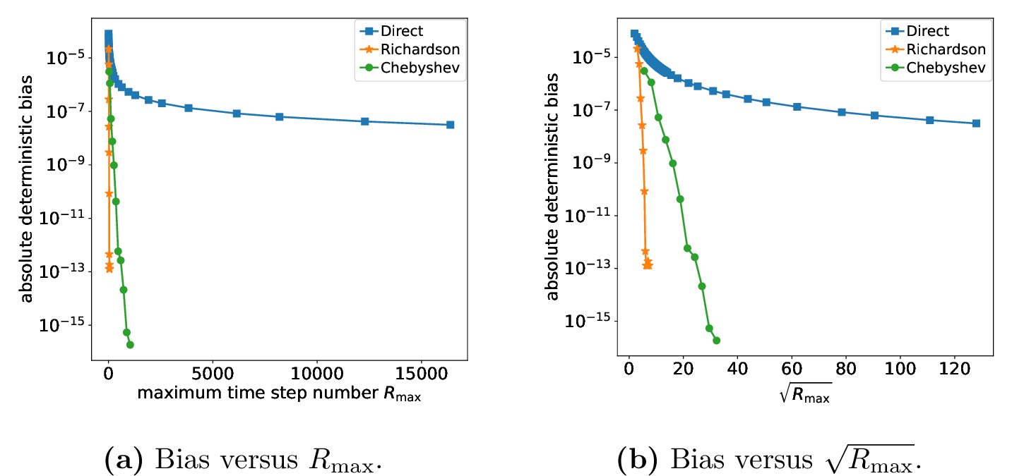
2 shows the deterministic-bias reduction at fixed data points. The \(x\) axis is \(R_{\max}=\max_j R_j\), the maximum number of time steps among the finite-step circuits used in the extrapolation, where \(s_j=T/R_j\). The actual maximum single-run circuit depth is \[D_{\max}=d_{\rm step}R_{\max},\] up to lower-order measurement overheads. The \(y\) axis shows the absolute deterministic bias \[\left|g_O^{\rm approx}-g_O(0)\right|,\] where \(g_O(0)=\bra{\psi_0}(e^{TA})^{\dagger}O(e^{TA})\ket{\psi_0}\) is the exact zero-step reference and \(g_O^{\rm approx}\) is either the direct finite-step value or the extrapolated value. The direct method behaves as expected for a first-order discretization: decreasing the step size improves the error slowly. Richardson and Chebyshev both reduce the bias rapidly as the number of nodes increases. This supports the derivative-bound picture that \(g_O(s)\) is smooth enough near \(s=0\) for polynomial extrapolation to cancel or interpolate the leading step-size error terms.

At a higher degree, the Richardson curve can stop improving. This is expected in finite precision. If the computed scalar data are perturbed as \(\widetilde{g}(s_j)=g(s_j)+\xi_j,\) then the extrapolated perturbation is \(\sum_j a_j\xi_j,\) with bound \[\left|\sum_j a_j\xi_j\right|\le \Lambda_m\max_j |\xi_j|, \qquad \Lambda_m=\sum_j |a_j|.\] Richardson weights become increasingly oscillatory as \(m\) grows, so a small numerical perturbation can be amplified. Chebyshev interpolation has a milder weight growth in these tests and gives smoother high-degree behavior. This is why Chebyshev is the more stable choice when finite precision, node rounding, or finite-shot noise is present.

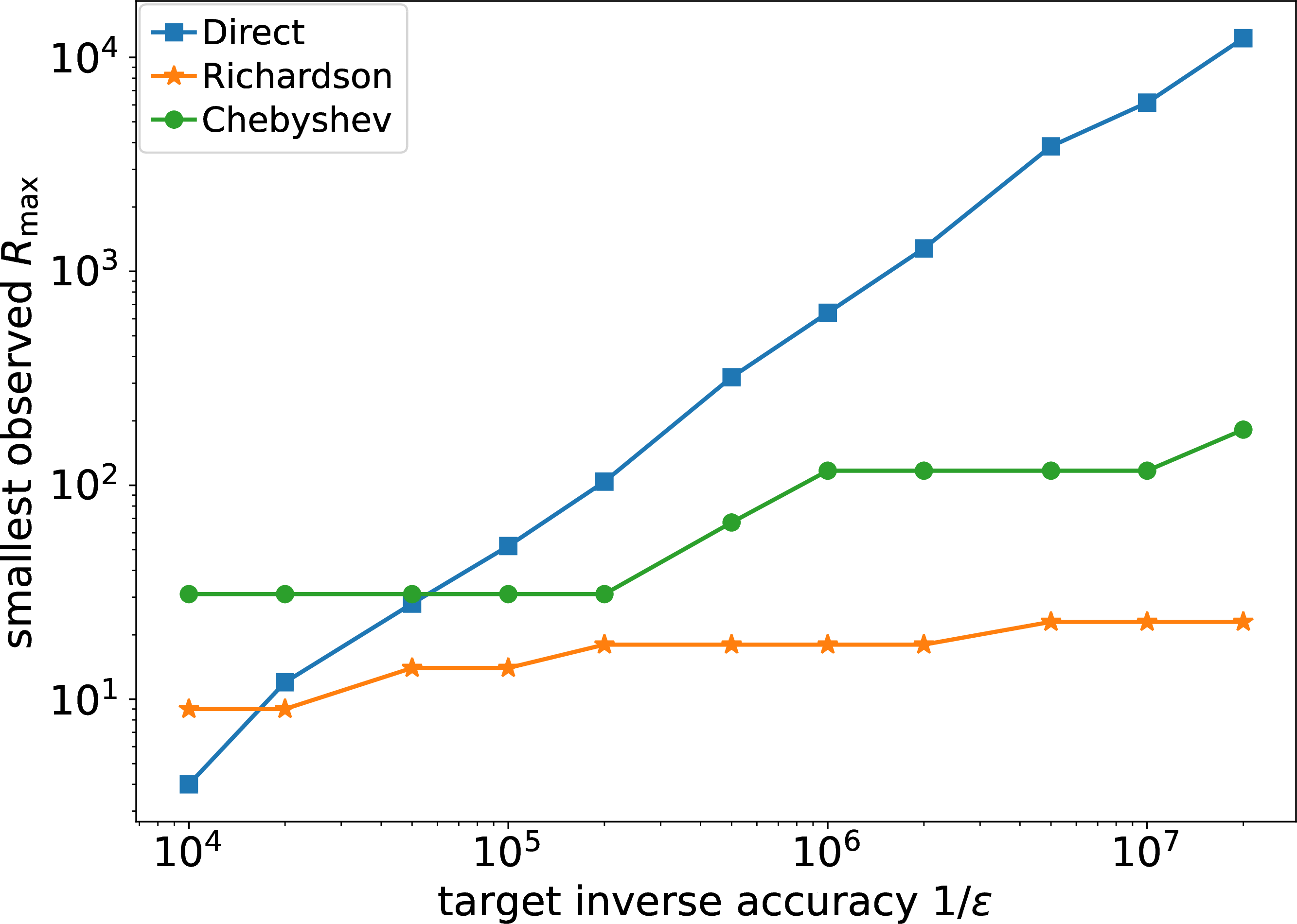
3 inverts the previous comparison. For each target accuracy \(\epsilon\), we record the smallest observed \(R_{\max}\) such that this precision is reached. The direct curve grows quickly as \(1/\epsilon\) increases, consistent with first-order accuracy. The Richardson and Chebyshev curves do not change much. In particular, they are step-like because both \(m\) and \(R\) are integer-valued, but they remain far below the direct curve in the high-accuracy regime. The last visible upward step in the Chebyshev curve is a degree-selection effect. In the Hatano-Nelson data, the \(m=4\) Chebyshev interpolant has \[R_{\max}=117, \qquad E\approx 5.30\times 10^{-8}.\] It satisfies all targets down to \(\epsilon=10^{-7}\), but it does not satisfy the stricter target \(\epsilon=5\times 10^{-8}\). The selected degree then increases to \(m=5\), giving \[R_{\max}=182, \qquad E\approx 7.53\times 10^{-9}.\] The jump \(117\to 182\) is therefore not an instability. It reflects the discrete change in \(m\) and the relation \(R_{\max}=\Theta(m^2)\).

5.2 Convection-Diffusion Equation↩︎

The second benchmark is a two-dimensional periodic convection-diffusion equation, \[\partial_t c(x,y,t)=-\nabla\cdot\left(v(x,y)c(x,y,t)\right)+\nu\Delta c(x,y,t).\] In the numerical example, we choose the following parameters \[v(x,y)=\alpha(\sin y,\sin x), \quad \alpha =1.2, \quad \quad \nu=\frac{1}{2}, \quad T=0.75.\] The equation is discretized on a \(6\times 6\) Fourier spectral grid. We note that this small-sized discretization is only meant for demonstration purposes. The initial condition is a normalized Gaussian on the torus, namely, \[c_0(x,y) = C\exp\left( -\frac{ d_{\rm torus}(x,\pi/2)^2+d_{\rm torus}(y,\pi/2)^2 }{2\sigma^2} \right), \qquad \sigma=0.55,\] where \(C\) is chosen so that \(\|c_0\|_2=1\), and \[d_{\rm torus}(a,b) = \min\{|a-b|,\;2\pi-|a-b|\}.\] The observable is the low-Fourier-shell projector \[O_{\rm low}=\sum_{0<|k|\le 2}|k\rangle\langle k|.\] This observable measures the unnormalized low-frequency content of the solution. We perform similar numerical tests to the Hatano-Nelson model for the convection-diffusion equation.

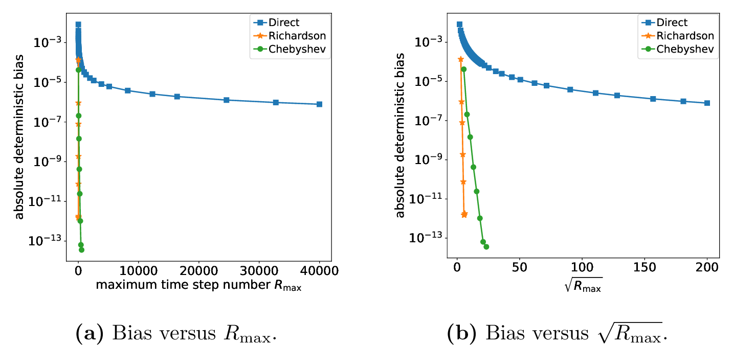
4 shows that the extrapolation mechanism is consistent with the theory. The convection-diffusion observable also exhibits rapid bias reduction under Richardson and Chebyshev postprocessing. The plotted extrapolated curves use \(m=2,\ldots,9\). This range shows the deterministic decay regime before the high-degree numerical floor dominates the experiment. The direct method remains much larger over the same range of maximum step numbers.

5 gives the required-depth comparison for the PDE observable. The direct method requires rapidly increasing \(R_{\max}\) as the target accuracy is tightened. In the plotted range, it reaches \(R_{\max}=32768\) for \(\epsilon=10^{-6}\). The extrapolated methods need much smaller depth. The Chebyshev curve has a visible step because the selected degree changes discretely. In this data set, the \(m=2\) Chebyshev interpolant has \[R_{\max}=29, \qquad E\approx 4.20\times 10^{-5}.\] It satisfies targets down to \(\epsilon=5\times 10^{-5}\), but not the target \(\epsilon=2\times 10^{-5}\). Increasing to \(m=3\) gives \[R_{\max}=63, \qquad E\approx 2.07\times 10^{-7}.\] The jump \(29\to 63\) is therefore a degree-selection effect. It is consistent with the Chebyshev relation \(R_{\max}=\Theta(m^2)\), since the factor is close to \((3/2)^2\) up to rounding from the constraint \(s_j=T/R_j\).

6 Conclusion and Remarks↩︎

In this work, we use classical step-size postprocessing techniques to reduce the circuit depth of the one-ancilla quantum differential equation solver. We show that both Richardson extrapolation and Chebyshev interpolation can substantially reduce the maximum single-run circuit depth. Compared with directly using the finite-step solver, the maximum depth per run improves from \(\mathcal{O}(1/\epsilon)\) to \(\mathcal{O}(\mathop{\mathrm{polylog}}(1/\epsilon))\) in the target accuracy \(\epsilon\), up to problem-dependent prefactors. While Richardson extrapolation exhibits a faster initial convergence rate, Chebyshev interpolation offers better numerical stability. Consequently, the preferred choice in practice depends on the target accuracy regime and the specific error and stability considerations of the application. Quantitatively, Richardson’s extrapolation weights grow exponentially in the number of nodes, while Chebyshev’s grow only polylogarithmically, after accounting for the discreteness of realizable step sizes. These scalings are consistent with the numerical experiments.

From a technical standpoint, a core ingredient distinguishing this work from existing literature on time-step extrapolation lies in handling the adjoint operators inherent to differential equations. We successfully addressed this challenge by introducing the holomorphic lift framework, bridging the gap between extrapolation techniques and general quantum ODE simulations.

This work demonstrates how classical postprocessing can be systematically combined with quantum circuits to mitigate quantum resource overheads for linear differential equations. Such a perspective may be naturally extended to other quantum differential equation solvers to achieve improved quantum estimates. The one step block underlying the present algorithm achieves only first order accuracy in the step size, and whether a post selected construction with higher order accuracy exists, compatible with the present extrapolation framework, remains open. Ultimately, validating the feasibility and robustness of this protocol on actual quantum hardware platforms remains an important and interesting future direction.

7 Acknowledgement↩︎

This work is supported by the U.S. Department of Energy, Office of Science, Accelerated Research in Quantum Computing Centers, Quantum Utility through Advanced Computational Quantum Algorithms, grant no. DE-SC0025572. We also acknowledge the support from the National Science Foundation CAREER Award DMS-2438074.

8 Chebyshev Node Identities↩︎

This appendix establishes the two trigonometric identities used to bound the Chebyshev node products and reciprocal sums in 11. Let \(T_n\) denote the degree \(n\) Chebyshev polynomial of the first kind, satisfying \(T_n(\cos \alpha)=\cos(n\alpha)\), with leading coefficient \(2^{n-1}\) for \(n\ge 1\), and satisfying Chebyshev’s differential equation \[(1-x^2)T_n''(x)-xT_n'(x)+n^2T_n(x)=0.\] Fix \(m\ge 1\) and write \(\theta_\ell:=\frac{(2\ell-1)\pi}{4m}\) for \(\ell=1,\ldots,m\).

References↩︎