Physics-Audited Agentic Discovery in Scientific Machine Learning
July 08, 2026
Abstract
In agentic scientific machine learning (SciML), large language model (LLM) agents can discover surrogate models and select one by an automated score, typically an error metric. A low error, however, does not establish that the predicted fields satisfy the physics that matter for mechanics, such as boundary conditions, superposition, stiffness scaling, or causality. We introduce Physics-Audited Agentic SciML (PA-SciML), a verification-first workflow for agentic SciML discovery. The workflow fixes a scoring evaluator before search, derives reviewable machine-checkable physics requirements, checks each trained candidate on its outputs, and separately searches prescribed input ranges or measured load-history spans for high-violation cases without reference solution fields. A surrogate is reported as verified only under the stated checks. When enabled, the workflow also adds advisory numerical probes before training and tests one modeling change at a time to record which isolated edits are associated with score gains before reuse. In the reported computational-solid-mechanics numerical examples, the static elasticity run selects a surrogate with lower validation error than the error-only baseline while both selected models pass the common linear-elastic checks. In the transient elastodynamics run, an error-only baseline with similar mean error fails a stricter causality check by responding to future parts of the loading history, while the selected surrogate passes the stated checks. The main distinction is per-candidate physics evidence on predicted fields, not a richer aggregate score.
1 Introduction↩︎
Computational solid mechanics often requires repeated solutions to PDE-governed boundary-value and initial-boundary-value problems. Design sweeps, uncertainty quantification, inverse identification, and digital-twin workflows can require many evaluations of full displacement, stress, or history-dependent field responses. High-fidelity finite-element simulations remain the reference tool, but repeated solves can be too expensive when the geometry, material law, loading, or boundary data must be varied many times. Scientific machine learning (SciML) and neural-operator surrogates offer a complementary route: learn a map from problem inputs to solution fields so that a new case can be evaluated without a fresh finite-element solve [1]–[4]. The practical difficulty is that constructing a useful surrogate still depends on problem-specific choices of architecture, training strategy, physics-informed structure, and evaluation metric.
Large language model (LLM) agents are beginning to automate parts of this workflow. One branch writes and runs simulation code for finite-element mechanics and computational fluid dynamics [5]–[8]. Another branch automates engineering design and design review [9]. A third branch, closest to this paper, automates SciML model discovery: agents can propose surrogate designs, implement training code, critique candidates, and select models with limited human intervention [10]–[12], building on earlier automation of physics-informed network design [13], [14]. These systems make surrogate design less manual, but they also move a mechanics question to the center of the workflow: after an automated system selects a surrogate, what evidence shows that its predicted fields satisfy the physics the model is meant to emulate?
Score- or reward-mediated selection is not enough to answer that question. A validation error, training loss, or composite scientific reward can rank candidate models, but it does not necessarily check each trained surrogate’s outputs against machine-checkable physical requirements. Existing agentic SciML systems include important verification and diagnostic steps, but those checks are generally aimed at generated code, execution, plan consistency, or aggregate reward rather than at a separate output-level physics check on each scored surrogate [11], [12]. This is the gap addressed here. A selected surrogate may be plausible because it scores well, yet still lack direct evidence that its predicted fields obey the stated boundary, symmetry, scaling, or time-ordering requirements. The risk is also recognized in the agentic SciML literature: LLM-mediated debate may not reflect physically rigorous reasoning unless it is paired with numerical verification [10].
The gap is consequential in the numerical examples reported below, but in different ways across the two mechanics problems. In the static linear-elasticity example, a common post-run audit shows that both the audit-enabled selected surrogate and the error-only baseline satisfy the stated linear-elastic checks; there, the audit provides supporting evidence that the lower-error selected surrogate has not traded accuracy for violations of superposition, stiffness scaling, or roller boundary conditions. In the transient elastodynamics example, the distinction is decisive: rechecking an error-only baseline against a stricter causality requirement shows that it responds to future parts of the loading history. This is an output-level failure of the predicted field, not merely an implementation inconvenience. Together, the examples show why low error should not be read as evidence that a selected surrogate passes the stated physics checks.
We introduce Physics-Audited Agentic SciML (PA-SciML), a verification-first framework for agentic SciML discovery that adds per-candidate physics evidence to model selection. The framework is designed for agentic SciML more broadly; this paper demonstrates it on neural-operator surrogates for computational solid mechanics. PA-SciML fixes reviewable physics requirements before candidate search, scores every successful candidate with one fixed evaluator, applies sampled, machine-checkable physics checks to predicted outputs, and separately searches prescribed input ranges or measured load-history spans for high-violation cases without reference solution fields. A selected surrogate is reported as verified only under the stated checks. When enabled, the workflow also adds advisory pre-training numerical probes for proposed model changes and tests one isolated edit at a time to record the changes associated with score gains before reuse.
The contribution of this work is to make specified physics-check evidence part of the selection evidence for automated surrogate discovery. Rather than treating low validation error as sufficient, PA-SciML requires the predicted fields of a selected surrogate to pass prescribed machine-checkable physics checks in the stated verification setting. The numerical examples show two complementary roles for this evidence. In the static elasticity example, it documents that the selected lower-error surrogate remains consistent with the stated linear-elastic checks. In the transient example, it exposes a causality failure that the error metric misses. The same framework also records supporting evidence around the selection decision, including searches over admissible inputs without reference solution fields, advisory numerical probes before full training, and isolated-edit tests after discovery. This separation keeps failed execution, predictive error, physics-check results, and post-run analysis from being conflated.
The remainder of the paper is structured as follows: 2 situates PA-SciML within the SciML, neural-operator, agentic-discovery, and trustworthiness literatures; 3 details the framework and verification layer; 4 presents the experimental design and numerical examples; and [sec:discussion] [sec:conclusion] discuss limitations and outlook.
2 Related work↩︎
Scientific machine learning provides one route from repeated PDE solves to reusable surrogate models. Physics-informed neural networks embed governing-equation residuals in the training objective [1], while the broader physics-informed machine-learning literature shows how governing equations, boundary and initial conditions, conservation constraints, and data can be combined in neural models for forward and inverse PDE problems [2]. These works establish a foundation for physics-informed neural PDE solvers and surrogate models, but practical use still leaves problem-dependent choices: the architecture, residual weighting, training strategy, and the form in which physical information enters the model.
Neural operators and related full-field surrogates address the many-query setting by learning maps from problem inputs to solution fields. The theory behind this class of models includes universal approximation results for nonlinear operators [15] and the modern neural-operator framework, in which learned maps act between function spaces [16]. Two architectures anchor much of the field: DeepONet, which combines branch and trunk subnetworks [3], and the Fourier neural operator, which parameterizes an integral kernel in Fourier space [4]. Approximation-error estimates are available for DeepONet [17]. Both families have expanded in directions important for PDE surrogates: physics-informed operator learning adds residual-based constraints to the learned map [18], [19]; DeepONet variants include multiple-input operators [20] and comparative extensions benchmarked against Fourier neural operators [21]; and Fourier-operator variants address general geometries and multiphase-flow prediction [22], [23]. For this paper, the relevant design space includes both function-to-function operators and parameter- or load-to-field surrogates built from operator-learning architectures. Across that space, the architecture, physics-informed loss terms, geometry encoding, and data representation remain choices made for each problem.
In computational solid mechanics, learned surrogates have been developed for several physical tasks rather than a single model family. Constitutive and field-response surrogates cover path-dependent plasticity, thermo-viscoplastic transient material behavior, and full-field stress prediction [24]–[26]. Energy-based neural formulations have been introduced for finite-deformation hyperelasticity [27]. Operator-learning and parametric-PDE work covers fracture and damage, reduced models of input-output maps, nonlocal kernel networks, time-dependent input histories, and geometry-dependent full-field prediction [28]–[32]. A complementary finite-element-coupled line embeds neural networks inside finite-element solvers for nonlocal continuum damage and coupled multiphysics [33], [34], within a broader machine-learning and data-mining literature for continuum mechanics [35]. This literature demonstrates that surrogate models can represent rich mechanics responses, but it also illustrates why surrogate construction remains expert- and task-specific: each study must choose the architecture, training formulation, geometry representation, finite-element coupling, and physical structure appropriate to its problem.
Automating those modeling choices is therefore a natural next step. Auto-PINN searches over selected PINN architecture and hyperparameter choices using training loss as the search objective [36]. PINNsAgent uses Physics-Guided Knowledge Replay with Memory Tree Reasoning Strategy to optimize PINN architectures and hyperparameters [13], while Lang-PINN coordinates PDE, PINN, code, and feedback agents to turn natural-language task descriptions into executable PINN code with validation or feedback steps [14]. More recent agentic SciML systems broaden the search from tuning toward model and method discovery. AgenticSciML combines role-specialized agents, structured debate, retrieval of prior methods, and evolutionary search to generate and select SciML solutions [10]. ATHENA organizes numerical method discovery as an iterative propose-implement-evaluate process guided by expert-derived blueprints and a composite scientific reward [11]. GRAFT-ATHENA extends this direction toward cross-problem transfer through structured problem and method representations, metric neighborhoods, and reward-calibrated priors [12]. These systems indicate that agentic search can reduce manual method design. At the same time, their selection mechanisms are mediated by training loss, validation error, scientific reward, diagnostics, or trial history, rather than by a separate machine-checkable output test on each selected learned surrogate. AgenticSciML also identifies the underlying risk directly: LLM-mediated debate and justification may not reflect physically rigorous reasoning unless paired with numerical verification signals [10]. Reported error levels across this literature are regime-specific: canonical physics-informed PDE benchmarks, data-driven Burgers operator learning, and solid-mechanics surrogate learning differ in problem class, supervision, and metric [11], [12].
Language-model agents have also been applied to neighboring parts of the scientific and engineering pipeline. Agents can write, run, or debug mechanics, finite-element, PDE, and OpenFOAM workflows [5]–[8]. Other systems address knowledge-guided engineering design and optimization [9], autonomous chemistry experiment planning [37], tool-augmented chemistry reasoning [38], and end-to-end AI research workflows [39]. These works are important context for agentic automation, but their main objects are simulation code, design candidates, laboratory actions, or research workflows, not the selection of learned SciML surrogates using machine-checkable physics evidence on their predicted fields.
The agentic workflows above draw on a broader LLM-agent literature. ReAct introduced interleaved reasoning and tool or environment actions [40]. Multi-agent debate studies answer refinement through interaction [41]. CAMEL studies role-playing communicative agents [42], AutoGen provides a framework for composing conversational multi-agent workflows [43], and MetaGPT structures role-specialized collaboration through standardized operating procedures [44]. Reflexion uses verbal self-reflection over task feedback [45], and LLM-as-judge work studies model-based evaluation and its biases [46]. This machinery helps systems propose, coordinate, critique, and evaluate candidates. By itself, however, it does not establish whether a selected surrogate’s displacement, stress, or time-history fields satisfy the physics required by the mechanics problem.
This question connects agentic SciML to the trustworthiness literature. One strand builds physical information directly into model construction: governing-equation loss or likelihood terms can support label-free surrogate training [47]. Hard-constrained physics-informed neural networks can enforce constraints in inverse design for topology optimization [48], and conservation laws or other analytic constraints can be built into neural-network architectures or loss functions [49]. Another strand analyzes trained neural networks after training. Formal-verification tools can prove specified input-output properties or return counterexamples for supported ReLU or piecewise-linear networks [50], [51]; adversarial-robustness work studies worst-case input perturbations and robust-optimization formulations [52], [53]; and uncertainty-quantification methods estimate predictive uncertainty in neural SciML models, including PDE and operator-learning settings [54]. Together, these areas show that physical constraints can be built into learning and that trained networks can be checked, probed, or equipped with uncertainty estimates. What remains missing in the agentic SciML discovery line surveyed above is a workflow that applies machine-checkable output-level physics checks to each scored learned surrogate, separately searches the prescribed input set for large violations without reference solution fields, and reports the selected surrogate using that evidence rather than only an aggregate reward, training loss, or validation-error objective. The framework we present next addresses that gap.
3 Framework↩︎
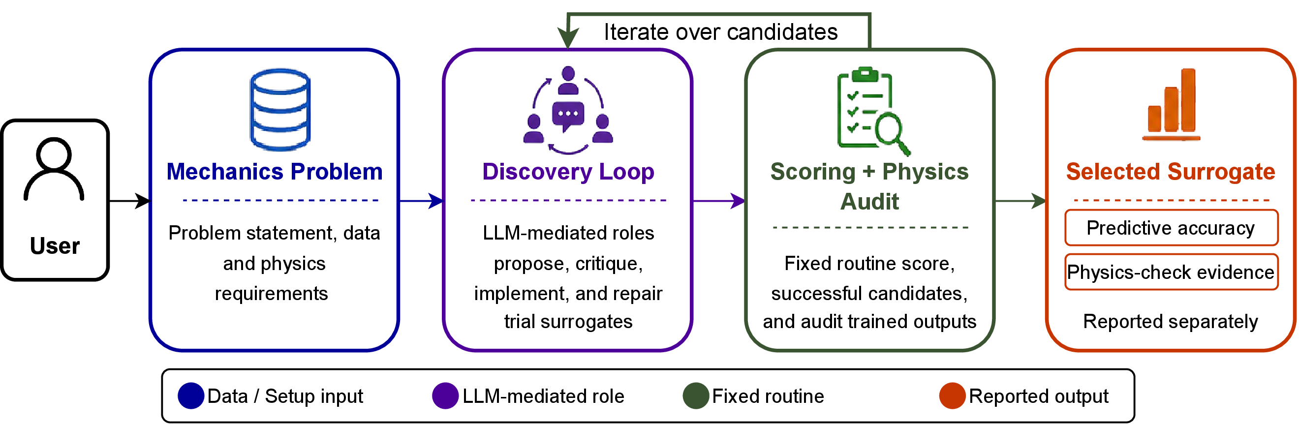
Physics-Audited Agentic SciML (PA-SciML) is a framework for discovering scientific machine learning (SciML) surrogates for mechanics problems while reporting predictive accuracy separately from specified physics-check evidence. 1 gives a high-level overview and 2 summarizes the full workflow; 1 2 list the LLM-mediated roles and the fixed routines that score, check, and report candidates. The method is organized into three parts: the Discovery loop, the Verification layer, and Post-discovery attribution with Method-card saving. Executability checks within Candidate search and a complete run record run across all three, keeping execution failure separable from predictive error and physics-check behavior. The Discovery loop has two parts: setup and Candidate search. The run begins from user-specified problem information: the problem statement, data description, admissible input domain, and scoring target. Setup reads that information and fixes the derived records used later, including the data summary, Fixed evaluator, and, when auditing is enabled, physics contracts. Candidate search generates, trains, scores, and records trial surrogates in a Candidate search tree. The Verification layer defines the stated physics checks, applies them to trained candidate outputs through the Physics audit, and uses the Sampled hard-contract gate to report a selected surrogate under those checks. Post-discovery attribution and Method-card saving optionally test isolated edits associated with score gains and save a reusable method card when the required checks pass; the candidate that produced the method card is also recorded. Thus, LLM-mediated roles help explore surrogate designs, while fixed routines produce the evidence used for scoring, physics checking, and final reporting.
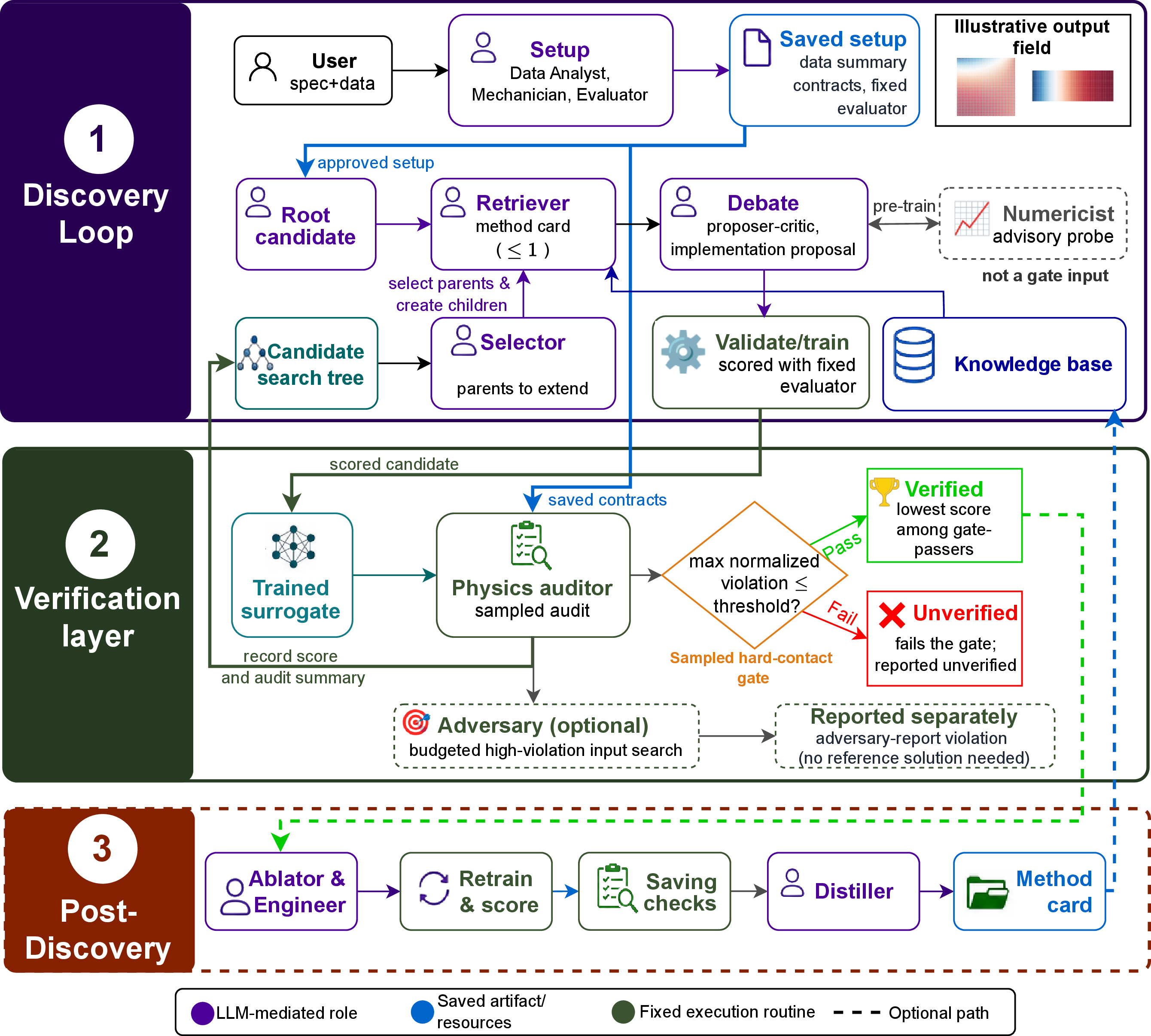
| Role | Purpose | Role | Purpose | |||
|---|---|---|---|---|---|---|
| Data analyst | Summarizes the available data and problem context for setup. | Proposer | Suggests candidate model changes during Candidate search. | |||
| Evaluator | Drafts the predictive scoring routine that becomes the Fixed evaluator for comparing candidates. | Critic | Reviews proposed changes before implementation. | |||
| Mechanician | Selects supported physics-check types and proposes their parameters, labels, and tolerances from the supplied problem statement and setup-generated calibration evidence. | Engineer | Implements proposed trial surrogates and repair edits. | |||
| Root engineer | Builds the first trial surrogate from the original specification. | Debugger | Diagnoses candidate failures for bounded repair attempts. | |||
| Retriever | Selects at most one saved method card when retrieval is enabled. | Selector | Chooses which scored candidate to extend next. | |||
| Result analyst | Summarizes candidate predictions, scores, and physics-check evidence. | Ablator | Decomposes improved changes into isolated edits for fixed retesting. | |||
| Distiller | Drafts a method card after the required score and audit checks pass and the candidate that produced the method card is recorded. |
| Routine | Purpose | |
|---|---|---|
| Fixed evaluator | Gives every successfully scored trial surrogate the same lower-is-better predictive score. | |
| Candidate validation and scoring routine | Checks that a candidate exposes the expected interface and can run, applies completeness and repair checks, trains it when possible, applies the Fixed evaluator, and records whether the attempt succeeded, so execution failure is not confused with prediction error. | |
| Physics Auditor | Applies the configured physics checks to predicted fields and records the maximum normalized violation, \(\violmax{}\), for audited candidates. | |
| Sampled hard-contract gate | Reports the lowest-score audited surrogate that passes the sampled hard physics checks; if none pass, the reported surrogate is marked unverified. | |
| Adversary | Optional high-violation input search called after the Physics audit; it keeps a trained surrogate fixed and varies admissible inputs to report large physics-check violations separately from the Sampled hard-contract gate. | |
| Numericist | Runs advisory numerical probes for proposed model changes before full training; these probes do not decide final reporting. | |
| Method-card saving rule | Check the required score improvement, the physics-check condition when required, and the evidence record before a method card is saved. |
3.1 Discovery loop↩︎
The Discovery loop constructs and tests trial surrogate models under one scoring rule. The run begins from user-specified problem information: the problem statement, data description, admissible input domain, and scoring target. During setup, the workflow reads that information, prepares a data summary, and builds and saves the Fixed evaluator before Candidate search begins. Here, fixed means that the Fixed evaluator is reused unchanged for candidate comparison; it is not a formal guarantee that the saved file could not later be changed or that the Fixed evaluator is independently correct. Predictive comparisons are therefore conditional on the Fixed evaluator and its validation data. 3 shows the setup and Candidate search path.
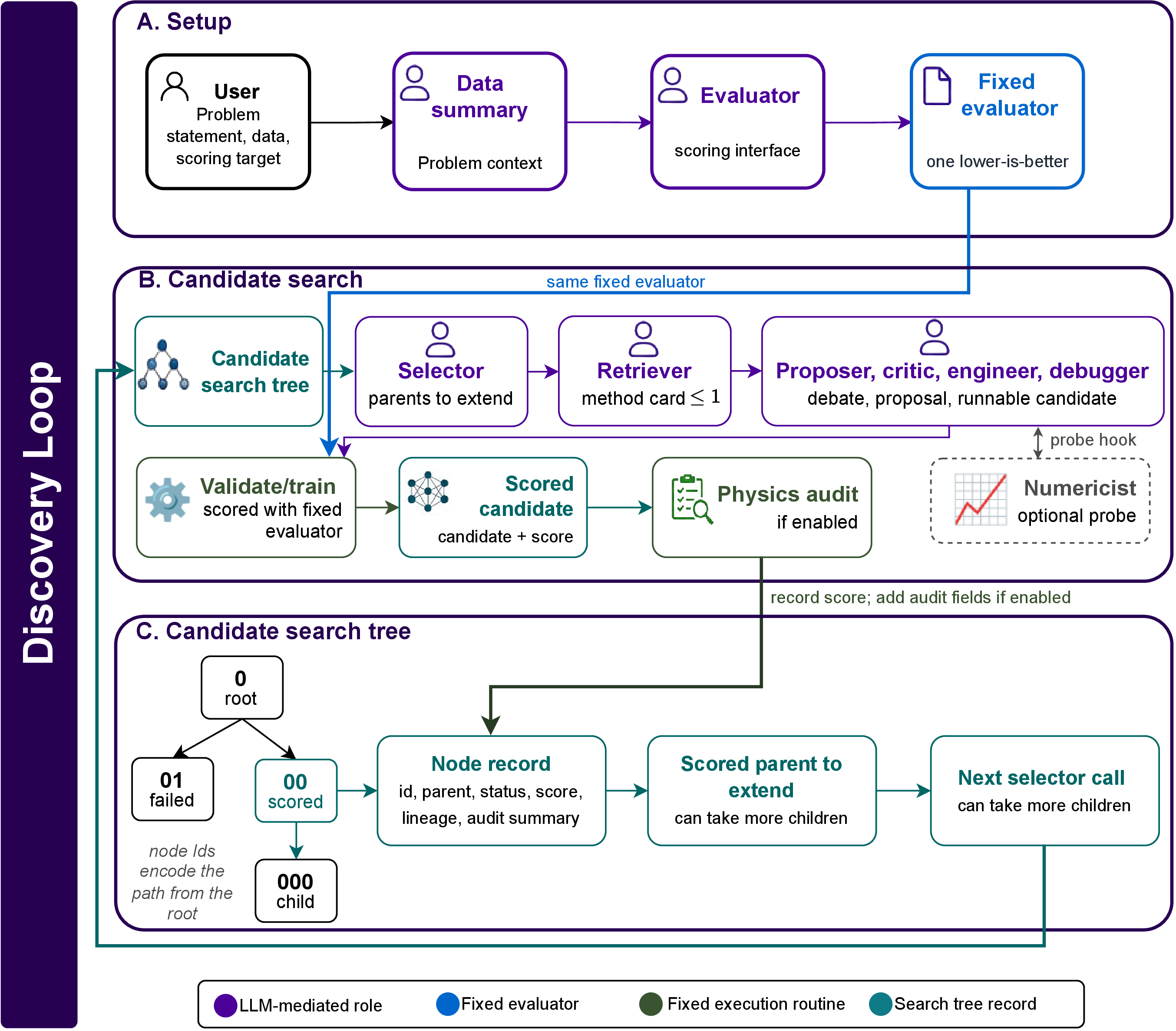
The Candidate search grows a Candidate search tree. The root candidate is generated from the supplied problem specification. Each later node is a child obtained by editing an already scored parent. The tree records lineage, status, score when available, and links to detailed run artifacts; it is a record of surrogate-design history, not a finite-element tree or a tree of solution fields.
The Candidate search separates LLM-mediated design from fixed evidence production. For each selected parent, the Proposer suggests a candidate modification and the Critic reviews it before implementation. The Engineer implements the plan; when validation or scoring fails, the Debugger attempts repairs. The workflow then validates the implementation, trains the candidate, and scores it with the Fixed evaluator. Validation checks that the candidate exposes the expected prediction interface and that the Fixed evaluator can compute a scalar score; completeness and repair checks catch empty, truncated, syntactically invalid, or missing-entry-point implementations, and a candidate that cannot be scored is not used as a parent for later edits. When the run has more scored candidates than it can extend in the next iteration, the Selector chooses which parents to extend while retaining the current best candidate when it can still be extended by additional child candidates. The Retriever may supply one saved method card for the selected parent; if no suitable entry is selected, Candidate search proceeds without one. When enabled, the Numericist runs advisory numerical probes before full training; these probes are not physics contracts and do not enter the Sampled hard-contract gate.
Candidate scoring and physics verification are separate. Without a contract file, the workflow can still score and compare trial surrogates, but it does not report that the selected surrogate passed physics checks. With a contract file, recorded physics-check results can inform later choices about which candidate to modify, while the final selected-surrogate claim is governed by the Sampled hard-contract gate defined in the next subsection. These results do not change the debate that produced the audited candidate. Instead, they are stored in the candidate record and summarized in later reports for related candidates, so later Proposer, Critic, and, when retrieval is enabled, Retriever steps can use the previous physics-check behavior.
3.2 Verification layer↩︎
When auditing is enabled, problem-specific physics requirements are encoded as contracts. The Verification layer denotes the full set of choices and routines used to produce physics evidence; the Physics audit is the fixed-code, per-candidate execution of the sampled contract checks within that layer. A contract is a typed physics-check specification interpreted by routines that are part of the framework implementation and supplied before the run. It is not executable check code written by an LLM-mediated component or newly written for each candidate. The contract file selects a supported check type and supplies its parameters, severity, and tolerance. Hard-contracts gate verified selected-surrogate reporting; soft contracts are recorded only as diagnostics. The admissible input domain for audit is denoted \(\mathcal{Z}\). It is a space of problem inputs, such as parameters or load histories, not the spatial body \(\Omega\) and not a space of solution fields. A verification setting fixes the contract file, hard/soft labels, tolerances, sampling protocol, \(\mathcal{Z}\), reporting threshold, and, when enabled, the Adversary search settings. Unless explicitly qualified as an Adversary report or reference audit, verified means passing the Sampled hard-contract gate for that setting. This is in-domain, contract-bounded evidence, not a proof outside \(\mathcal{Z}\). 4 summarizes the in-run Physics audit and Sampled hard-contract gate, followed by the separate optional Adversary report and any post-run reference-audit reports.
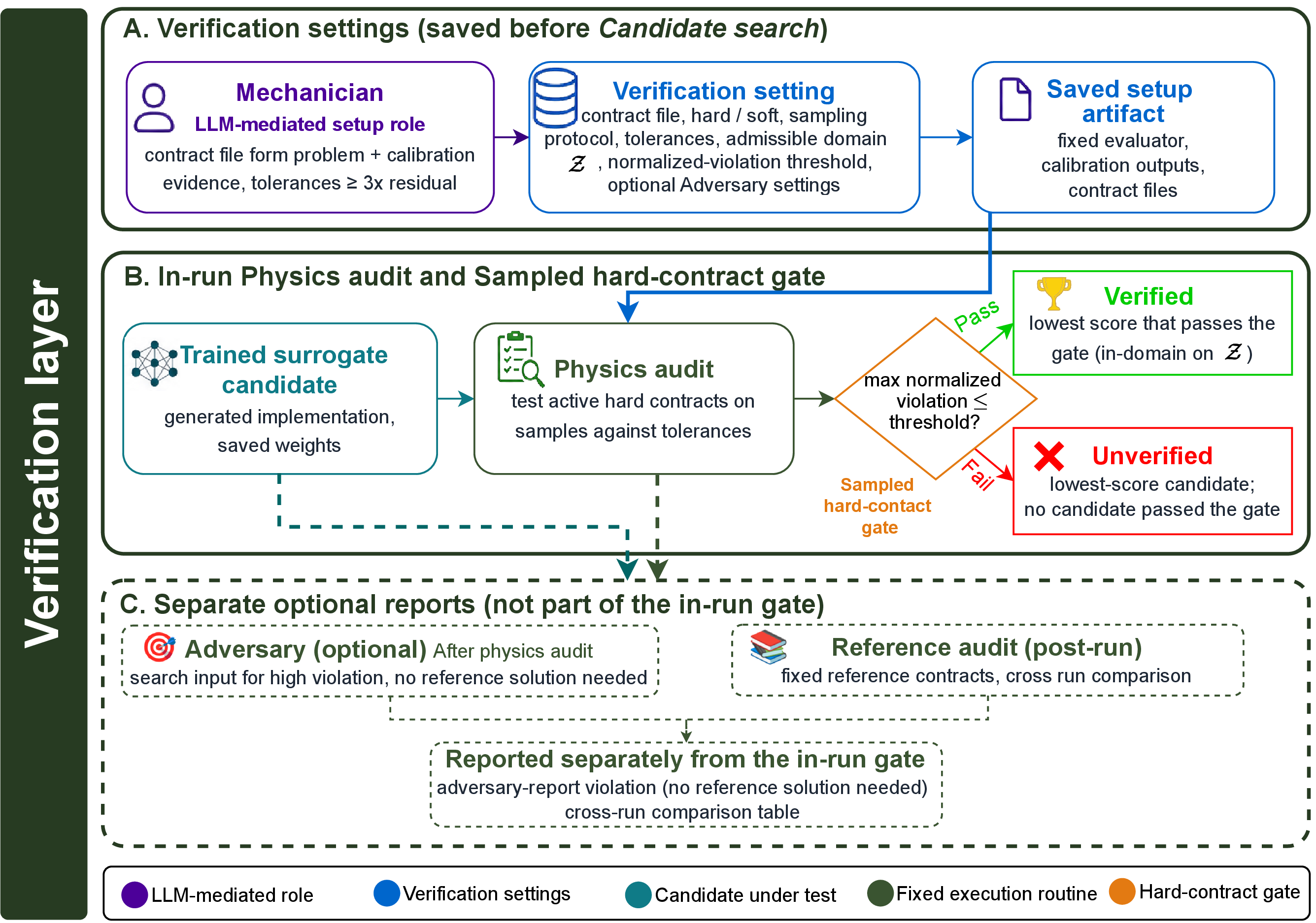
In audited runs, a scored candidate is checked only when a valid score and contract file are present. The Physics audit checks active hard contracts on finite probes drawn from, constructed within, or specified in \(\mathcal{Z}\). Skipped hard checks are reported but excluded, so a pass is a pass over active, non-skipped hard checks. Audit failures do not count as passes. After this sampled audit, the optional Adversary can run a high-violation input search for hard checks with implemented search objectives and directly compute hard checks where implemented, without reference solution fields. Disabling this search removes the separate Adversary report, but it does not change the Physics audit, \(\mathrm{viol}_{\max}{}\), or the in-run Sampled hard-contract gate. Post-run reference audits are also separate verification settings and do not redefine the in-run Sampled hard-contract gate.
Contracts and the Mechanician. Supported contracts cover check families implemented in the framework, such as linearity or scaling, symmetry or antisymmetry, boundary or initial-condition consistency, output bounds, and temporal-consistency checks. These families are not universal mechanics assumptions: the contract file should include only properties valid for the governing regime, inputs, and outputs being audited. Shared names may have mode-specific meanings, for example finite-dimensional parameter checks versus function-valued input checks. Appendix 7 gives a catalogue of implemented checks.
During setup, an LLM-mediated setup component, the Mechanician, drafts the contract file from the supplied problem statement and calibration evidence generated before any candidate surrogate is trained. The Mechanician does not write executable check code; it chooses among the supported check types and proposes their parameters, hard/soft labels, and tolerances, which are then interpreted by the fixed audit routines. Calibration estimates residual or scale levels for available probes; it is not a constitutive fit and not a residual estimate for every possible contract. The workflow prompts the Mechanician to choose tolerances no tighter than \(3\times\) measured calibration residuals when such residual evidence exists. This \(3\times\) rule is guidance during contract proposal, not an automatically enforced validity guarantee. Tolerances, hard/soft labels, and the input domain are therefore setup assumptions of the verification setting and are archived for review.
Before Candidate search begins, the Fixed evaluator, calibration outputs, and contract file are saved and reused during Candidate search. Post-run comparison audits may rerun the in-run contract file or alternative files on existing selected surrogates, but they do not validate calibration-to-tolerance choices. A check can be soft in one setting and hard in another, so PASS/FAIL labels and rounded violations must be read with the contract file that produced them.
Fixed-code physics checks. The Physics audit runs no LLM-written contract-checking code. The trained surrogate is the object under test: each check calls the candidate only through its input-output map, such as input parameters or load histories in and predicted fields out. Thus the checking and aggregation logic are fixed, while the generated surrogate implementation and learned weights are treated as the surrogate being audited. The resulting evidence concerns the predicted fields under the specified checks.
For each active hard contract \(c\), the Physics audit applies the check to a finite probe set \(\mathcal{S}_c\) and computes a dimensionless violation \(v_c(q)\) for each probe \(q\). The sampled hard-contract statistic is \[\begin{align} \mathrm{viol}_{\max}{} = \max_{c \in \mathcal{H}} \frac{\max_{q \in \mathcal{S}_c} v_c(q)}{\tau_c}. \end{align} \label{eq:violmax}\tag{1}\] where \(\tau_c>0\) is the contract tolerance and \(\mathcal{H}\) is the non-empty set of active hard contracts after skipped checks are removed. A candidate passes the Sampled hard-contract gate when \(\mathrm{viol}_{\max}{}\) is no larger than the configured reporting threshold. If no hard contract remains active, the Physics audit reports no Sampled hard-contract gate pass.
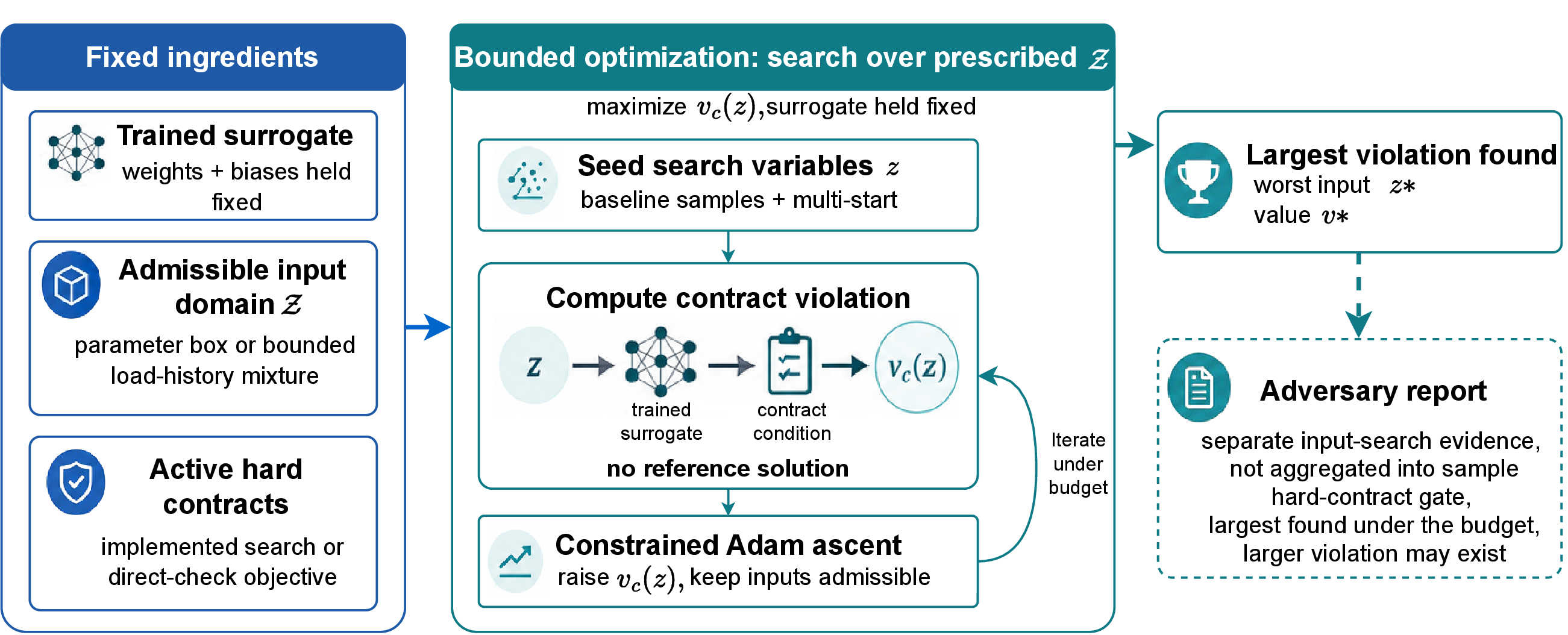
Physics Auditor, Adversary, and Sampled hard-contract gate. The Physics Auditor is the fixed audit routine that computes sampled contract results for scored candidates and stores compact audit summaries in the Candidate search tree; full results remain in the run artifacts. It is not an LLM agent. The optional fixed high-violation search routine, the Adversary, is called after the Physics audit when enabled (5). Its search objectives and direct-check routines are part of the framework implementation and are available only for selected hard-check types. It keeps the trained surrogate fixed: the learned weights and biases are not updated. Here, bounded means that the search is restricted to the prescribed admissible input domain \(\mathcal{Z}\): it varies only the input-side search variables \(z\) that parameterize admissible probes and maximizes the corresponding contract violation \(v_c(z)\). In the reported runs, this optimization seeds the search variables from baseline samples and multiple starts, then raises the violation by constrained Adam ascent while keeping the constructed inputs admissible. For parameter-vector inputs, the variables are normalized coordinates in the prescribed box; for function-valued inputs, they are bounded mixture coefficients over admissible load histories. Its objective uses surrogate outputs and contract conditions, not reference solution fields. Direct hard checks are computed where implemented; hard checks without an implemented search or direct-check routine are not included in the largest violation reported by the Adversary. The report gives the largest violation found under the chosen budget and parameterization; it does not prove that larger violations are absent.
Values from Adversary reports, soft diagnostics, and post-run reference audits are reported separately from the in-run Sampled hard-contract gate. At final reporting, an audit-enabled run selects the lowest-score candidate among those with sampled \(\mathrm{viol}_{\max}{}\) no larger than the configured threshold; if no candidate passes, it reports the lowest-score candidate as unverified. The run may also report a Pareto front in the score and violation plane: among candidates with both a score from the Fixed evaluator and a sampled \(\mathrm{viol}_{\max}{}\), the front contains those for which no other candidate has both a lower score and a lower violation.
3.3 Post-discovery attribution and method-card saving↩︎
Post-discovery attribution asks whether a child’s score gain can be reproduced by one isolated edit after Candidate search. 6 traces the optional path from an improving parent–child edge through single-edit retraining tests to the checks that decide whether a method card is saved. A saved method card can be retrieved in later Candidate search runs.
The attribution routine, called the Ablator, uses an LLM to split an improving parent–child code change into at most \(K\) testable edits. For each parsed edit, the Engineer creates a parent-code variant containing only that edit, and fixed routines retrain and rescore the variant under the same Fixed evaluator. For parent score \(s_{\mathrm{parent}}\), child score \(s_{\mathrm{child}}\), and single-edit score \(s_{\mathrm{edit},i}\), define \(g=s_{\mathrm{parent}}-s_{\mathrm{child}}\) and The largest \(\phi_i\) is reported as an operational share of the gain, not causal proof. The corresponding interaction residual is a score-space diagnostic, not a governing-equation residual. Retraining noise and edit interactions can make \(\phi_i<0\) or \(\phi_i>1\).
Method-card saving is independently enabled. The Distiller uses an LLM to draft the method-card text only after the required saving checks pass: a successful child with valid parent and child scores, sufficient relative improvement, dominant single-edit share of at least \(0.5\), no existing method card for that candidate, and audit pass when required. Fixed code validates required metadata, records the candidate that produced the method card and the supporting evidence, and saves the method card. Adversary reports are not part of the Method-card saving rule unless explicitly cited.
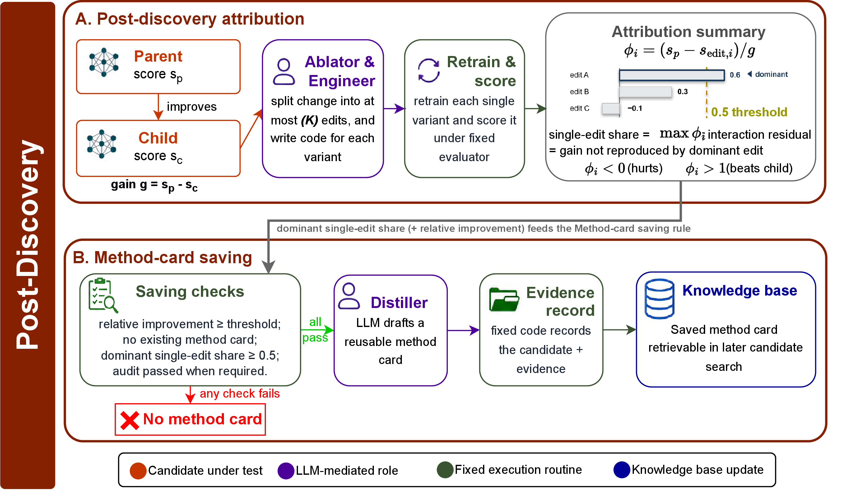
The in-run contract file and any post-run comparison contract file are separate verification settings. Likewise, Post-discovery attribution provides evidence rather than causal proof: ablation results show how isolated edits perform under retraining, and any saved method card records the candidate it came from and the checks that supported saving it, so the method card can be retrieved in a later search.
3.4 Reproducibility and traceability↩︎
Each run preserves a complete record: the Fixed evaluator, the contract file when used, the search and audit budgets, candidate lineage, candidate implementations, logs, scores, and audit summaries. This record is what lets execution failure, predictive error, and physics-check behavior be told apart; the executability and repair checks described in 3.1 produce the failed-run status that the record distinguishes from a genuine physics pass or fail.
The record establishes only that a candidate ran and was scored; it does not establish physical validity. The Fixed evaluator provides predictive-error evidence, while the Physics audit provides physics-check evidence by applying fixed routines to contracts proposed during setup by the Mechanician. Metric-parity checks can rerun the Fixed evaluator on an archived candidate to verify score compatibility, but they do not provide evidence of mechanics. The numerical examples specify domains, budgets, contract inventories, baseline definitions, and result values.
4 Numerical examples↩︎
4.1 Common setup and reporting↩︎
Each numerical example follows the same reporting protocol. We first specify the governing boundary-value or initial-boundary-value problem, the admissible inputs, the solution field to be approximated, the reference data, and the physical requirements used to check the predicted field. The inputs may be loads, source terms, boundary data, material parameters, or load histories, depending on the problem. Before Candidate search begins (3.1), the run fixes one lower-is-better Fixed evaluator; every successfully trained surrogate in that example is scored by this same evaluator. When auditing is enabled, the run also fixes the physics-check specification for the stated verification setting (3.2). Trial surrogates are then trained, scored, and, where applicable, checked under prescribed computational budgets. The run record preserves the predictive score, the physics-check summary, and how each trial surrogate is related to earlier attempts.
All predictive comparisons are within-example comparisons. A raw score in one problem should not be read against a score in another, because each problem has its own field scale, validation data, and Fixed evaluator. Physics claims are likewise local to the check specification and verification setting that produced them. Post-run reference audits can compare already trained selected surrogates under a common set of checks, but those audits are separate verification settings; they do not change the live Sampled hard-contract gate, the pass or fail rule that compares each candidate’s largest tolerance-normalized hard-check violation with a fixed threshold (1 ). Each example therefore reports both the predictive accuracy of the selected surrogate relative to reference solution fields and whether its outputs satisfy the stated physical checks.
4.2 Parametric linear elasticity↩︎
The first numerical example concerns a small-strain, two-dimensional linear-elastic body occupying \(\Omega=[0,1]^2\). The material response is parameterized by Young’s modulus and Poisson ratio. Let \(\mathbf{u}=(u_x,u_y)\) denote the displacement, \(\boldsymbol{\varepsilon}\) the infinitesimal strain, and \(\boldsymbol{\sigma}\) the Cauchy stress. In the absence of body forces, the static boundary-value problem has the standard form \[\begin{align} \nabla\!\cdot\boldsymbol{\sigma} &= \mathbf{0} && \text{in } \Omega, \\ \mathbf{u} &= \bar{\mathbf{u}} && \text{on } \Gamma_u, \\ \boldsymbol{\sigma}\cdot\mathbf{n} &= \bar{\mathbf{t}} && \text{on } \Gamma_t, \end{align}\] where \(\Gamma_u\) and \(\Gamma_t\) denote displacement and traction boundaries and \(\mathbf{n}\) is the outward unit normal. The small-strain kinematics and isotropic constitutive relation are \[\boldsymbol{\varepsilon}(\mathbf{u}) = \tfrac12\left(\nabla\mathbf{u}+(\nabla\mathbf{u})^{T}\right), \qquad \boldsymbol{\sigma}=\mathbb{C}(E,\nu):\boldsymbol{\varepsilon}. \label{eq:elastic-constitutive}\tag{3}\] Here \(\mathbb{C}(E,\nu)\) denotes the isotropic elastic stiffness associated with the \(E,\nu\) material parameterization. The domain is discretized on a fixed mesh of 2601 nodes. The loading is a uniform traction \(\bar{\mathbf{t}}=(f_x,f_y)\) on the top edge \(y{=}1\), where \(f_x\) is the tangential component and \(f_y\) the normal component, each in \([-0.3,0.3]\). The material parameters vary over \(E\in [5,20]\) and \(\nu\in [0.15,0.35]\), and the left edge \(x{=}0\) is traction-free. Roller supports fix the normal displacement on the other two edges: the bottom edge has zero vertical displacement, \(u_y=0\) on \(y{=}0\), and the right edge has zero horizontal displacement, \(u_x=0\) on \(x{=}1\). The tangential displacement component on each roller-supported edge is free to slide and varies with the loads applied on the top edge. The finite-element reference data, surrogate output, and validation target all contain both displacement components. The surrogate maps the four scalars \(\mathbf{z}=(f_x,f_y,E,\nu)\) to the full displacement field \(\mathbf{u}=(u_x,u_y)\) at the mesh nodes. Therefore, both roller conditions, \(u_x=0\) on the right edge and \(u_y=0\) on the bottom edge, enter the physics checks. 7 summarizes the domain, the top-edge traction, and the roller supports.
![Figure 7: Parametric linear elasticity: domain and boundary conditions. The unit square \Omega=[0,1]^2 is an isotropic linear-elastic solid with material parameters E and \nu. A uniform traction \bar{\mathbf{t}}=(f_x,f_y) is applied on the top edge y{=}1, with f_x the tangential and f_y the normal component, each varying over [-0.3,0.3] across samples (red arrows show one representative direction). The left edge x{=}0 is traction-free and there is no body force. Roller supports fix the normal displacement on the other two edges, u_y=0 on the bottom edge y{=}0 and u_x=0 on the right edge x{=}1, leaving the tangential component free to slide. The surrogate predicts both displacement components, so both roller conditions enter the physics checks.](/article/2607.07379/figures/elasticity_domain.png "fig:")
The mechanics of this problem impose simple but important structure on the predicted field. For fixed material parameters, linear elasticity gives traction superposition: the displacement produced by two applied tractions together should equal the sum of the two separate displacement fields. For fixed traction and \(\nu\), scaling \(E\) by a factor \(c\) should scale the displacement field by \(1/c\). The full displacement field should also reverse sign when both traction components are reversed, and it should satisfy the two roller constraints. A scalar predictive-error score does not enforce these properties. In this example, the reference audit is used primarily as a consistency check: it asks whether the audit-enabled search preserves these linear-elastic requirements while matching the error-only comparison, not whether the error-only selected surrogate is physically inadmissible.
4.2.0.1 Reference data and metric.
The reference displacement fields are finite-element solutions on the fixed mesh described above. The dataset contains 4000 training cases and 1000 held-out validation cases. The predictive metric is the mean per-sample relative \(L^2\) error of the full displacement vector \((u_x,u_y)\) on the validation set (\(\text{rel-}L^2\), lower is better). This Fixed evaluator is saved before Candidate search and reused unchanged for every comparison. Because relative error can be sensitive when the reference displacement is very small, we also report percentile and worst-case errors.
4.2.0.2 Selected surrogate.
The audit-enabled run selected a physics-structured DeepONet whose architecture carries the linear-elastic structure of the problem by construction (8). The branch network receives only the Poisson ratio; the traction components and Young’s modulus enter through the fixed compliance prefactors \(f_x/E\) and \(f_y/E\), which multiply four branch heads, one pair per displacement component; and two coordinate factors that vanish on the roller edges multiply the assembled output, as shown in [lst:elasticity-champion]. Consequently, load superposition and reciprocal \(E\) scaling hold for any value of the trained weights; reversing both traction components reverses the predicted displacement field; and the two roller conditions are satisfied identically. Training determines only the Poisson-ratio dependence of the four head fields and the spatial basis supplied by the trunk. Concretely, the branch maps the normalized Poisson ratio through three \(256\)-wide tanh layers with a skip connection into four bias-free linear heads, each producing \(p=64\) coefficients; the heads that couple \(f_y/E\) to \(u_x\) and \(f_x/E\) to \(u_y\) carry the Poisson coupling between the load direction and the transverse response. The trunk evaluates \(17\) fixed features of the coordinates, nine polynomial and eight sinusoidal terms, and passes them through a \(256\)-wide residual network of three blocks with tanh activations into two bias-free heads that supply \(64\) spatial basis functions per displacement component; each predicted component is the inner product of its coefficient and basis vectors, multiplied by the roller factor and a fixed per-component output scale. The model has about \(6.3\times10^{5}\) trainable parameters. In mechanics terms, the model is a discrete superposition representation, \(\mathbf{u} = (f_x/E)\,\mathbf{G}_x(\nu) + (f_y/E)\,\mathbf{G}_y(\nu)\), with \(\mathbf{G}_x\) and \(\mathbf{G}_y\) learned unit-load response fields over the mesh. None of this structure was prescribed: the problem specification fixes only the branch-trunk product form and the two-component output, and the candidate search introduced the factorization at its first improving step, as the isolated-edit comparison below records.
![Figure 8: Selected surrogate for the parametric elasticity example: a physics-structured DeepONet. Blue boxes are the trained networks; neutral boxes are fixed by construction and carry the linear-elastic structure. The branch turns the Poisson ratio into four head fields A,B,C,D, and the fixed compliance prefactors f_x/E and f_y/E assemble coefficients that are linear in the loads, so, for any trained weights, load superposition and reciprocal-E scaling hold, and reversing both traction components reverses the predicted displacement field. The trunk turns 17 fixed coordinate features, nine polynomial and eight sinusoidal, into the spatial bases \Phi_{u_x} and \Phi_{u_y}. After the coefficient-basis inner product, the roller factors, (1-x) on u_x and y on u_y, enforce u_x=0 at x{=}1 and u_y=0 at y{=}0 identically, and a fixed per-component scale sets the output amplitude. The assembled model is the discrete superposition \mathbf{u}=(f_x/E)\,\mathbf{G}_x(\nu)+(f_y/E)\,\mathbf{G}_y(\nu) with learned unit-load response fields \mathbf{G}_x, \mathbf{G}_y, and has about 6.3\times10^{5} trainable parameters. [lst:elasticity-champion] shows the corresponding listing.](/article/2607.07379/figures/elasticity_surrogate.png "fig:")
Listing lst:elasticity-champion: Listing for the selected surrogate of the parametric elasticity example, showing the load and material factorization. Input normalization, device handling, and output scaling are omitted. The branch sees only the Poisson ratio; the loads and Young's modulus enter through compliance prefactors, and coordinate factors impose the roller conditions identically.
fx, fy = params[:, 0:1], params[:, 1:2]
E,  nu = params[:, 2:3], params[:, 3:4]
fx_over_E, fy_over_E = fx / E, fy / E      # loads enter only as fx/E, fy/E
A, B, C, D = self.branch(nu_norm)          # branch input: Poisson ratio only
coeff_ux = fx_over_E * A + fy_over_E * B   # linear in (fx, fy) by construction
coeff_uy = fx_over_E * C + fy_over_E * D   # reverses sign when loads reverse
ux = einsum('bp,mp->bm', coeff_ux, trunk_ux_basis)  # DeepONet inner product
uy = einsum('bp,mp->bm', coeff_uy, trunk_uy_basis)
ux = ux * (1.0 - x)                        # right-edge roller: ux = 0 at x = 1
uy = uy * y                                # bottom-edge roller: uy = 0 at y = 0
4.2.0.3 Physics checks.
The physics checks encode these linear-elastic consequences as finite-sample tests on predicted displacement fields. In the live audit-enabled run, the hard checks are load superposition, reciprocal \(E\) scaling, the bottom-edge \(u_y\) condition, the right-edge \(u_x\) condition, and sign reversal under load reversal; an amplitude bound is recorded as a soft diagnostic. For the common post-run comparison below, the reference checks use four hard requirements: load superposition, reciprocal \(E\) scaling, right-edge \(u_x\), and bottom-edge \(u_y\). Load-sign reversal is reported separately as a diagnostic because, in this linear-elastic setting, it follows from the same linearity that gives load superposition. The amplitude bound is also reported as a diagnostic. Thus, each pass/fail label and normalized violation should be read together with the particular set of checks used to produce it (3.2).
4.2.0.4 Accuracy.
On the held-out displacement fields, the selected surrogate from the audit-enabled run attains a \(\text{rel-}L^2\) of 8.864 × 10⁻⁵. The error-only baseline, selected by predictive error alone with physics checks switched off during Candidate search, reaches 2.103 × 10⁻⁴. The selected surrogate’s worst validation case (1.376 × 10⁻⁴) and \(95\)th-percentile error (1.249 × 10⁻⁴) are also lower than the baseline values (3.376 × 10⁻⁴ and 3.148 × 10⁻⁴, respectively; 3). These values are a single-run comparison between two independently discovered surrogates, not a variance-estimated accuracy claim. The selected surrogate and this error-only baseline were scored by the same held-out relative-error evaluator. The validation error distribution of the selected surrogate is narrow, with mean 8.864 × 10⁻⁵, median 9.331 × 10⁻⁵, and maximum 1.376 × 10⁻⁴ (9 (a)). 10 shows the displacement-magnitude fields behind these numbers: in each case the displacement is largest near the top-left corner, where the loaded top edge meets the traction-free left edge, and the predicted \(|\mathbf{u}|\) is in good agreement with the reference from the \(10\)th to the \(90\)th error percentile. The gain is consistent with the isolated-edit evidence reported below: the dominant improving edit is the physics-structured factorization described above (5).
| Surrogate | val.p95 | val.max | sampled | Adversary | status | |
|---|---|---|---|---|---|---|
| Selected surrogate | 8.864 × 10⁻⁵ | 1.249 × 10⁻⁴ | 1.376 × 10⁻⁴ | 1.708 × 10⁻⁴ | 2.087 × 10⁻³ | pass |
| Error-only baseline | 2.103 × 10⁻⁴ | 3.148 × 10⁻⁴ | 3.376 × 10⁻⁴ | 1.080 × 10⁻³ | 2.582 × 10⁻³ | pass |
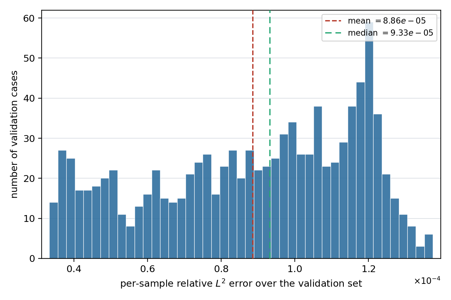
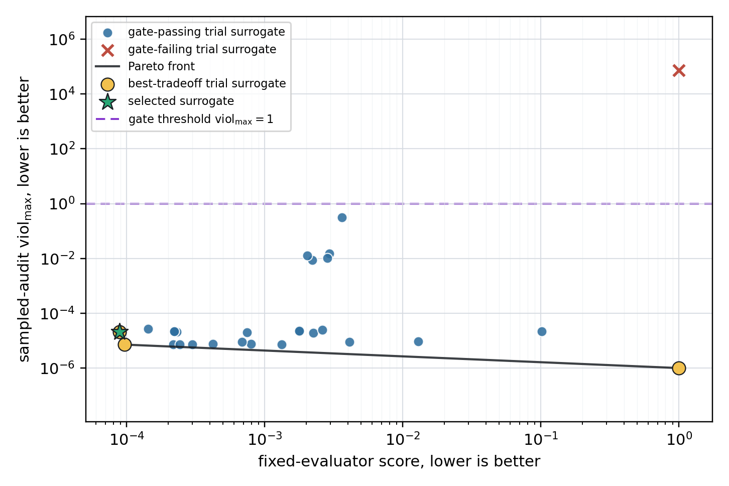
Figure 9: Parametric linear elasticity, selected surrogate diagnostics. (a) Distribution of the per-sample relative \(L^2\) error of the selected surrogate over the 1000 validation cases (mean 8.864 × 10⁻⁵, median 9.331 × 10⁻⁵, maximum 1.376 × 10⁻⁴). (b) Predictive error against worst sampled physics violation for every successfully scored and audited trial surrogate in the Candidate search, on logarithmic axes; the dashed line is the Sampled hard-contract gate threshold (\(\mathrm{viol}_{\max}{}=1\)). The selected surrogate (star) has the lowest error among gate-passing candidates. The only gate-failing candidate is also a high-error trial surrogate. Sampled violations of exactly zero are plotted at the axis floor of \(10^{-6}\) so that they appear on the logarithmic scale. Panel (b) uses live sampled audit values from the Candidate search; 3 reports the separate common reference audit for the selected models..
![Figure 10: Parametric linear elasticity: displacement-magnitude fields of the selected surrogate. Reference (top row) against selected-surrogate prediction (bottom row) of the displacement magnitude |\mathbf{u}| over the unit square \Omega=[0,1]^2, for the validation cases at the 10th, 50th (median), and 90th percentiles of the per-sample relative L^2 error (n=\num{1000}); each column header gives the selected case’s error. The two panels of a column share one color scale, with the power-of-ten factor above the bar. In every case the displacement is largest near the top-left corner, where the loaded top edge meets the traction-free left edge, and the prediction is in good agreement with the reference across the distribution, consistent with the narrow error distribution in 9 (a).](/article/2607.07379/figures/field_quantiles_elasticity.png "fig:")
4.2.0.5 Physics verification.
The physics checks test the predicted displacement fields directly for the linear-elastic structure stated above; they use no reference solutions. Re-checking the same models against the common reference checks, without retraining, shows that both surrogates pass the stated hard checks (3 4). The normalized violations are all at least two orders of magnitude below the pass threshold, and most are much smaller. The error-only baseline’s largest sampled value comes from reciprocal \(E\) scaling, while the selected surrogate’s largest sampled value comes from load superposition. These small quantities should not be read as a mechanically meaningful advantage of one model over the other. Both correspond to raw residuals near the single-precision noise floor, well below each model’s own predictive error, so the gap between them carries no physical information. For the selected surrogate, the checked properties hold by construction, as described above, and the audit confirms that the exported trained model preserves them under the reference routines. The error-only baseline likewise carries the loads linearly by construction and imposes the roller conditions through boundary factors; its reciprocal \(E\) dependence is partly learned, and the training data reduce that scaling residual to about 1 × 10⁻⁵ in relative terms. The Adversary, the separate no-reference high-violation input search that holds each trained surrogate fixed and varies only admissible inputs, confirms that the largest violations it finds remain far below the pass threshold for both models (5). Thus, this example is a no-failure verification case: the audit documents that the more accurate selected surrogate still satisfies the stated linear-elastic checks, while the decisive pass/fail contrast is provided by the transient example below.
| Check | severity | selected surrogate | error-only baseline |
|---|---|---|---|
| load superposition | hard | 1.708 × 10⁻⁴ / 2.087 × 10⁻³ | 9.46 × 10⁻⁵ / 3.03 × 10⁻⁴ |
| \(1/\Emod\) scaling | hard | 0 / 0 | 1.080 × 10⁻³ / 2.582 × 10⁻³ |
| right-edge | hard | 0 / 0 | 0 / 0 |
| bottom-edge \(u_y\) | hard | 9.83 × 10⁻¹⁵ / 1.44 × 10⁻¹⁴ | 9.87 × 10⁻¹⁵ / 1.45 × 10⁻¹⁴ |
| load-sign reversal | soft\(\dagger\) | 0 / n.a. | 0 / n.a. |
| amplitude bound | soft\(\dagger\) | 0 / n.a. | 0 / n.a. |
4.2.0.6 Candidate search.
The audit-enabled run generated 28 trial surrogates. All 28 were scored and audited; 27 passed the live Sampled hard-contract gate, and the one failure is a degenerate candidate whose predicted field collapsed toward zero, rejected with a normalized violation four orders of magnitude above the threshold. The error-only run also generated 28 successfully scored trial surrogates, but physics checks were switched off during its Candidate search. The error-versus-violation plot in 9 (b) therefore summarizes the audit-enabled search: the selected surrogate is the lowest-error candidate among those passing the live gate, while the single failed candidate has a score near one and is not competitive by predictive error. In this example, the live gate does not change the low-error selection; it mainly records that the selected surrogate satisfies the stated checks.
4.2.0.7 Isolated-edit comparison.
An improving step in the candidate search usually changes several things at once, for example the architecture, the training schedule, and implementation details. The isolated-edit comparison asks, after the search, which single change mattered. This follows the Post-discovery attribution procedure in [sec:attribution-method-card-saving] 6; the reported share is the single-edit quantity \(\phi_i\) in 2 . Each improving step on the path to the selected surrogate is split into its individual edits; each edit is applied on its own to the starting model of that step, and the resulting variant is retrained and rescored under the same fixed metric. Four improving steps were examined this way (5). Only the first gave a clear answer: replacing a generic branch network with the physics-structured factorization described above recovers, by itself, more than the entire improvement of that step, which means the changes made alongside it were neutral or harmful. This edit was saved as a method card, a reusable design note that later discovery runs can retrieve. The three later steps did not reduce to one change: their edits improve the score only in combination, the leading edit of one step worsens the score when applied alone, and the leading edits of the final two steps recover less than half of their steps’ gains. We therefore treat only the physics-structured factorization as a reusable lesson from this example.
| Improvement step | saved isolated edit | share of gain |
|---|---|---|
| first improvement | physics-structured DeepONet branch | 149% |
4.2.0.8 What this example shows.
Taken together, the example teaches two things. First, the audit-enabled run reached the more accurate surrogate in this comparison, and the physics evidence shows that this accuracy is not obtained by sacrificing any stated physical requirement. Second, and independent of the accuracy outcome, the audit changes what is known: both surrogates satisfy the stated linear-elastic checks, but without the audit that statement would be unavailable for either of them, because a low predictive error alone says nothing about superposition, stiffness scaling, or the roller conditions. The transient example that follows provides the complementary case, in which the same reporting protocol exposes an accurate error-selected surrogate that violates a hard physical requirement.
4.3 Transient elastodynamics↩︎
The second numerical example concerns a thin rectangular linear-elastic body in the transient regime. The strip \(\Omega = [-0.5, 0.5] \times [-0.1, 0.1]\) (length \(1\), height \(0.2\)) has material properties that are fixed for every sample, Young’s modulus \(E= 10\), Poisson ratio \(\nu= 0.25\), and density \(\rho = 1\) in consistent units, and is discretized with second-order triangular finite elements on a mesh with 4681 nodes. Starting from zero initial displacement and velocity, the solid is driven by a prescribed motion of its right edge; the left edge is fixed, and the long edges are traction-free (11). With the small-strain kinematics and isotropic constitutive relation of 3 , here under plane stress, the displacement field \(\mathbf{u}(\mathbf{x}, t) = (u_x, u_y)\) obeys \[\begin{align} \rho\,\ddot{\mathbf{u}} &= \nabla\!\cdot\boldsymbol{\sigma} && \text{in } \Omega \times (0, T], \\ \mathbf{u}(\mathbf{x}, 0) &= \mathbf{0}, \quad \dot{\mathbf{u}}(\mathbf{x}, 0) = \mathbf{0} && \text{in } \Omega, \\ \mathbf{u} &= \mathbf{0} && \text{on the left edge } x = -0.5, \\ \mathbf{u} &= \bar{\mathbf{u}}(t) && \text{on the right edge } x = +0.5, \\ \boldsymbol{\sigma}\cdot\mathbf{n} &= \mathbf{0} && \text{on the long edges } y = \pm 0.1, \end{align}\] with \(T = 2\) and no body force. The prescribed motion \(\bar{\mathbf{u}}(t) = (\bar{u}_x(t), \bar{u}_y(t))\) translates the right edge as a whole: it is uniform along the edge and varies only in time. The input supplied to the surrogate contains four time-series channels sampled at 100 uniform steps over \(t \in [0, T]\): the prescribed edge displacements \(\bar{u}_x, \bar{u}_y\) and the corresponding velocity channels. The displacement channels define the boundary motion; the velocity channels are the corresponding time derivatives supplied as additional input information, not independent boundary conditions. The surrogate maps this boundary-motion history to the full transient displacement field \((u_x, u_y)\) at every node and time. Thus the surrogate input is a sampled function of time, and inertia enters the balance of momentum.
![Figure 11: Transient elastodynamics: domain and boundary conditions. The thin strip \Omega=[-0.5,0.5]\times[-0.1,0.1] is an isotropic linear-elastic solid in plane stress with material properties fixed for every sample, E=10, \nu=0.25, and \rho=1 in consistent units; only the loading history varies between samples. The left edge x{=}{-}0.5 is fully fixed, u_x=u_y=0. The right edge x{=}{+}0.5 follows a prescribed time-dependent motion \bar{\mathbf{u}}(t)=(\bar u_x(t),\bar u_y(t)) over t\in[0,2], uniform along the edge so the edge translates as a whole; the red arrows show the two motion components. The long edges y{=}{\pm}0.1 are traction-free, and the body starts from rest, with zero initial displacement and velocity. The surrogate maps this right-edge motion history to the full transient displacement field (u_x,u_y).](/article/2607.07379/figures/elastodynamics_domain.png "fig:")
Disturbances excited at the moving right edge propagate along the strip and reflect from the fixed left edge, so the response at any node is a history-dependent superposition of traveling waves. Beyond spatial boundary and linearity checks, this problem therefore adds a temporal requirement with no static analogue: causality. For a transient elastic solid starting from rest, the displacement at time \(t\) may depend on the boundary motion up to \(t\), but it should not depend on motion prescribed later in the history. A surrogate trained and scored on complete trajectories can have a low mean error while failing this forward-in-time requirement.
4.3.0.1 Reference data and metric.
The reference trajectories are transient finite-element solutions on the fixed mesh described above, and the held-out validation set contains 500 load histories. Candidates are ranked by the fixed accuracy measure for this example: the mean relative \(L^2\) error over the complete displacement history and all mesh nodes. Because the body starts from rest, the field norm is small at early times; relative errors there are less physically informative than errors after the response develops. We therefore report the mean error together with the \(95\)th-percentile and maximum validation errors. All accuracy and physics checks below use the same 500 validation histories. In the post-run reference audit, both surrogates are re-evaluated with the same fixed accuracy routine; the recomputed mean errors reproduce their discovery-run scores, confirming that the comparison uses one validation set and one accuracy measure. The common reference audit uses only the physics checks reported below.
4.3.0.2 Selected surrogate.
The audit-enabled run selected a DeepONet with a causal load branch and a factorized space-time trunk (12). The branch encodes the four input channels through a causal convolution: the history is padded on the left, so the branch coefficients at time \(t\) see only the prescribed motion up to \(t\), and the branch carries no bias, so the response is linear in the load history and reverses sign when the prescribed motion is reversed. The output adds two parts: a lifting term, linear in \(x\), that carries the prescribed motion exactly on the right edge and vanishes on the fixed left edge, and a learned correction multiplied by an envelope that vanishes at \(t=0\) and on the left and right edges ([lst:elastodynamics-champion]). Causality, load linearity, amplitude scaling, sign symmetry, zero response to zero input, and the two displacement boundary conditions therefore hold by construction for any trained weights, and the zero initial state follows because the envelope vanishes at \(t=0\) and every admissible history starts from rest. Training determines the temporal kernels of the branch and the spatial and temporal bases of the correction. Concretely, each displacement component has its own single-layer causal convolution, a bank of \(p=32\) learned kernels spanning the full \(100\)-step window over the four input channels; each branch coefficient is therefore a discrete hereditary integral of the loading history, the counterpart of the Duhamel convolution that gives the exact response of a linear transient system driven from rest. The correction basis is factorized per component: a spatial network maps the coordinates and their sinusoidal embeddings, with the \(y\) frequencies scaled by the strip’s five-to-one aspect ratio, through two \(192\)-wide tanh layers into \(32\) spatial functions, and a separate temporal network maps the time coordinate and its sinusoidal embedding through two \(160\)-wide tanh layers into \(32\) temporal functions; the space-time basis is their product. The model has about \(2.0\times10^{5}\) trainable parameters, and the prescribed motion enters the output twice, analytically through the lifting and causally through the branch. None of this structure was prescribed: the problem specification fixes only the operator’s input-output form and leaves the load-history encoder and the trunk decomposition open, and the candidate search introduced the causal branch together with the factorized space-time representation at its second improving step, as the isolated-edit comparison below records.
![Figure 12: Selected surrogate for the transient elastodynamics example: a DeepONet with a causal load branch and a factorized space-time trunk. Blue boxes are the trained networks, one per displacement component; neutral boxes are fixed by construction and carry the transient linear-elastic structure. The branches read the right-edge motion history through left-padded, bias-free causal convolutions, so the coefficients b_{u_x}(t) and b_{u_y}(t) depend only on past loading. They act as discrete hereditary (Duhamel) integrals, are linear in the loading history, and reverse sign when the prescribed motion is reversed. The per-component space-time basis is the product \Phi_i(x,y,t)=\varphi_i(x,y)\,\psi_i(t) of 32 learned spatial and temporal functions, giving the correction r_i=b_i\cdot\Phi_i. The output assembly adds a lifting term g=\alpha\,\bar{\mathbf{u}}, with \alpha=x+0.5, which reproduces the prescribed right-edge motion exactly at x{=}{+}0.5 and vanishes at the fixed left edge x{=}{-}0.5, to the correction gated by the envelope \tau(t)\,\beta(x), which vanishes at t{=}0 and on the left and right edges, so the correction cannot perturb the initial state or the displacement boundary conditions. Causality, load linearity, amplitude scaling, sign symmetry, zero response to zero input, the zero initial state, and the two displacement boundary conditions therefore hold for any trained weights. The prescribed motion enters the output twice, analytically through the lifting and causally through the branches, and the model has about 2.0\times10^5 trainable parameters. [lst:elastodynamics-champion] gives the corresponding listing.](/article/2607.07379/figures/elastodynamics_surrogate.png "fig:")
Listing lst:elastodynamics-champion: Listing for the selected surrogate of the transient example, showing the causal branch and boundary structure. Normalization and output scaling are omitted. Left padding makes the branch causal; the lifting carries the prescribed right-edge motion and vanishes at the fixed left edge; the envelope vanishes at $t=0$ and on the left and right edges.
x_pad = F.pad(load, (T - 1, 0))            # left-pad: only past load values in view
b_ux  = self.branch_ux(x_pad)              # causal Conv1d, no bias: linear and causal
trunk_ux = phi_ux * psi_ux                 # factorized spatial x temporal basis
r_ux  = einsum('btp,tnp->btn', b_ux, trunk_ux)  # learned correction field
alpha = x + 0.5                            # 0 at fixed left edge, 1 at moving right edge
g_ux  = alpha * u_bar_x                    # lifting: prescribed motion, exact at x = +0.5
envelope = tau * beta                      # zero at t = 0 and at x = -0.5, +0.5
ux = g_ux + envelope * r_ux
4.3.0.3 Physics checks.
The physics checks reflect the linear transient setting: superposition and amplitude scaling of load histories, sign symmetry, zero response to zero input, zero initial displacement, agreement with the prescribed right-edge motion, causality, and an amplitude bound. The calibration evidence recorded before any surrogate was trained shows that the initial displacement is exactly zero at every node and sample, and that the reference right edge tracks its prescribed displacement channels to a maximum residual of 1.6 × 10⁻⁷, about 2 × 10⁻⁴ of the prescribed-motion scale. The live verification setting treated five checks as hard: superposition, amplitude scaling, sign symmetry, zero output for zero input, and zero initial displacement. It recorded midpoint causality and prescribed-right-edge consistency as soft diagnostics. The head-to-head comparison below uses a common reference set in which causality and the prescribed right edge are hard, while sign symmetry is soft. This gives six hard checks, each gated at a \(5\)% normalized tolerance. Each check defines a dimensionless raw violation, for example a relative \(L^2\) difference for superposition or a response-normalized residual for the zero-input check, which is then divided by the check tolerance; Appendix 7 catalogues the definitions. In the live run, causality was recorded but did not disqualify candidates. In the post-run comparison, both selected surrogates are checked again with causality treated as a hard requirement; the causality failure reported below comes from this common reference audit (3.2).
4.3.0.4 Accuracy.
On the held-out transient displacement fields, the selected surrogate attains a \(\text{rel-}L^2\) of 2.629 × 10⁻³, against 2.724 × 10⁻³ for the error-only baseline, about \(3.5\)% lower; its \(95\)th-percentile error (4.42 × 10⁻³) and worst validation case (5.48 × 10⁻³) are also below the baseline values (4.90 × 10⁻³ and 9.51 × 10⁻³, respectively; 6). The per-sample error distribution clusters near the mean, with only a small number of larger-error cases up to that worst case (13 (a)). 14 shows the field behavior behind these numbers: for a median-error case, the predicted and reference displacement histories at the node nearest the strip center are in good agreement and both build up from rest, consistent with the zero initial conditions (14 (a)), while the final-time displacement magnitude, largest in the interior of the strip, agrees from the \(10\)th to the \(90\)th error percentile, with visible discrepancy only in the hardest decile, concentrated where the field carries the most spatial structure (14 (b)). Enabling the physics checks therefore shows no accuracy penalty in this comparison.
| Surrogate | val.p95 | val.max | sampled | Adversary | status | |
|---|---|---|---|---|---|---|
| Selected surrogate | 2.629 × 10⁻³ | 4.42 × 10⁻³ | 5.48 × 10⁻³ | 0.00 | 0.00 | pass |
| Error-only baseline | 2.724 × 10⁻³ | 4.90 × 10⁻³ | 9.51 × 10⁻³ | 12.62 | 2750.62 | fail |
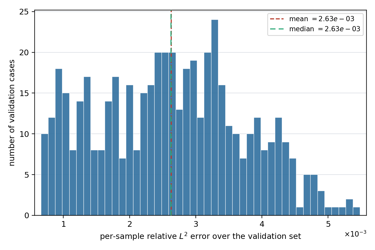
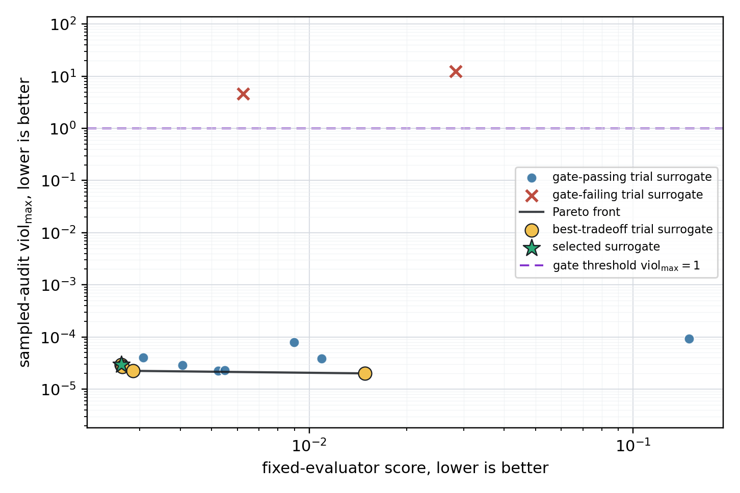
Figure 13: Transient elastodynamics, selected surrogate diagnostics. (a) Distribution of the per-sample relative \(L^2\) error of the selected surrogate over the full validation set (\(n=\num{500}\)) (mean 2.629 × 10⁻³, median 2.628 × 10⁻³, maximum 5.48 × 10⁻³); the error clusters near the mean, with a small number of larger-error cases up to the worst case. (b) Predictive error against worst sampled physics violation for every successfully scored and audited trial surrogate in the Candidate search, on logarithmic axes; the dashed line is the Sampled hard-contract gate threshold (\(\mathrm{viol}_{\max}{}=1\)). As in the first example, the selected surrogate (star) attains the lowest error with no reported violation at table precision, and nearly all trial surrogates satisfy the checks, so the tradeoff is governed mainly by predictive error. The accurate-but-acausal error-only baseline of 7 would lie far above the threshold. Panel (b) uses live sampled audit values from the candidate search; 6 reports the separate common reference audit for the selected models..
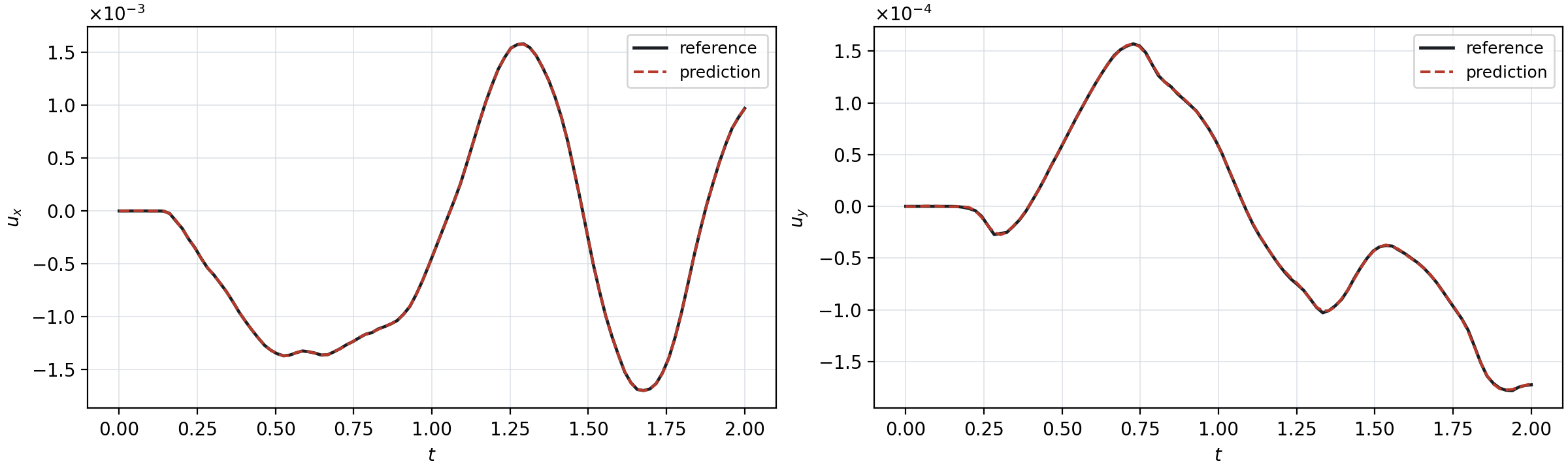
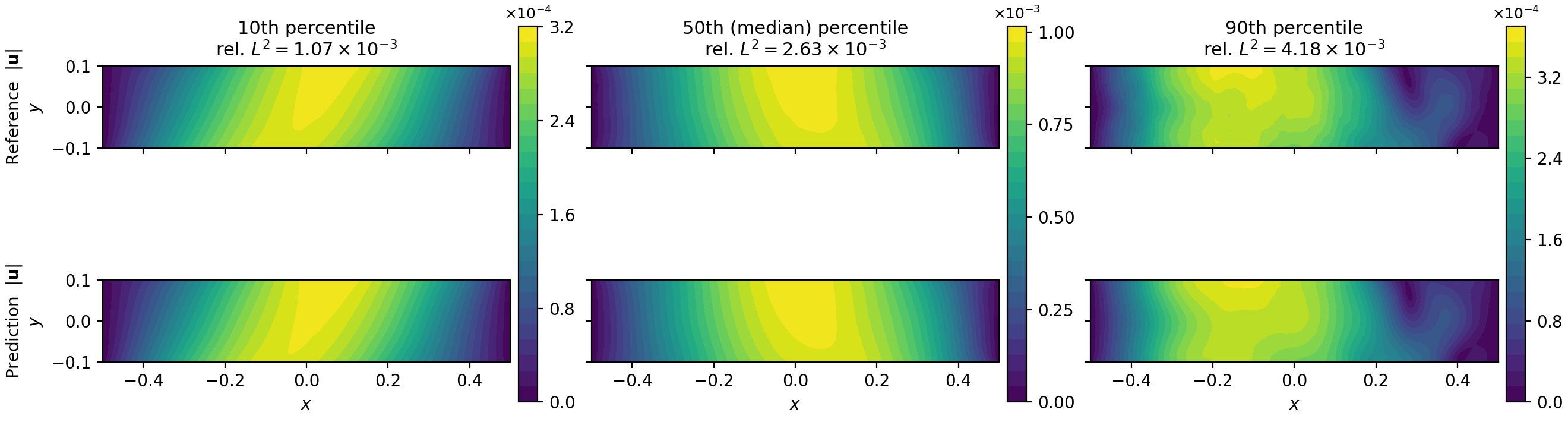
Figure 14: Transient elastodynamics: field behavior of the selected surrogate. (a) Reference (solid) and predicted (dashed) displacement histories \(u_x(t)\) and \(u_y(t)\) at the interior node nearest the strip center, for the median-error validation case (relative \(L^2\) 2.63 × 10⁻³); the curves are in good agreement and both build up from rest, consistent with the zero initial conditions. (b) Magnitude of the final-time displacement field \(|\mathbf{u}|\) over the strip, reference (top row) against prediction (bottom row), for the validation cases at the \(10\)th, \(50\)th (median), and \(90\)th percentiles of the per-sample relative \(L^2\) error (\(n=\num{500}\)); each column header gives the selected case’s error, and the two panels of a column share one color scale, with the power-of-ten factor above the bar. The prediction is in good agreement with the reference across the distribution, with visible discrepancy only in the hardest decile; 6 reports the corresponding aggregate statistics and physics checks..
4.3.0.5 Physics verification: causality.
Under the common reference set, the error-only baseline fails the reference physics checks for a forward transient surrogate: its predicted response before a given time changes when only later boundary motion is changed. The baseline uses a bidirectional load-encoding branch that reads the whole sequence, so early predictions can depend on later boundary motion. It breaches three hard checks in the Adversary report: causality (2750.62), load superposition (2.79), and the prescribed right edge (1.99), each above the normalized pass threshold of \(1\). The causality check is direct. It forms two boundary-motion histories that are identical up to the midpoint of the time window and differ only after that time. A causal forward surrogate should then predict the same displacement field before the midpoint for both histories. The error-only baseline does not. At sampled validation histories, the pre-midpoint displacement field changes by about \(63\)% in relative \(L^2\) norm; with a \(5\)% tolerance, this gives the sampled normalized violation 12.62. The separate input search holds the trained surrogate fixed and varies bounded mixtures of admissible load histories (5). It finds cases where the pre-midpoint response changes by more than one hundred times its norm, giving the reported value 2750.62. This dependence on future boundary motion is not visible in the mean error that selected the model.
The selected surrogate avoids this failure mode by construction, as described above: its causal branch cannot condition on future boundary motion. Its causality, zero-input, initial-condition, right-edge, and sign-symmetry violations are exactly zero under the reference routines, and its only nonzero values, 4.5 × 10⁻⁶ sampled and 6.7 × 10⁻⁵ under search on the load-linearity checks, sit at the arithmetic noise floor of single-precision superposition. The reference audit therefore separates two surrogates with similar predictive error by a mechanics requirement that is essential for forward transient prediction.
| Requirement | selected surrogate | error-only baseline |
|---|---|---|
| load superposition | 4.5 × 10⁻⁶ / 6.7 × 10⁻⁵ | 0.25 / 2.79 |
| amplitude scaling | 2.2 × 10⁻⁶ / 0 | 0.09 / 0.55 |
| zero input, zero output | 0 / 0 | 0.02 / 0.03 |
| zero initial displacement | 0 / 0 | 0.07 / 0.08 |
| causality | 0 / 0 | 12.62 / 2750.62 |
| prescribed right edge | 0 / 0 | 0.29 / 1.99 |
| sign symmetry\(\dagger\) | 0 / n.a. | 0.15 / n.a. |
| amplitude bound\(\dagger\) | 0 / n.a. | 0 / n.a. |
4.3.0.6 What the failure means.
A surrogate whose present response changes with future loading is not a valid forward model for settings in which the future load history is unknown. It is unsuitable for control, real-time estimation, or what-if prediction, because the computed displacement at the current time would depend on boundary motion that has not yet occurred. This failure is not apparent from a standard trajectory-error plot. When the complete load history is supplied, the error-only baseline can match the reference trajectory with low mean error; a single predicted trajectory does not show whether the same earlier response would be obtained if only the future part of the loading were changed. The causality distinction between the two surrogates therefore comes from the physics check.
4.3.0.7 Candidate search.
The search record is not the main evidence in this example, but it shows how often trial surrogates ran to completion and satisfied the in-run physics checks. Two of the 16 trial surrogates exceeded the training-time budget and did not produce usable scores. Of the 14 scored surrogates, 12 passed the Sampled hard-contract gate. The two in-run gate failures were trained surrogates with moderate predictive errors (scores 2.83 × 10⁻² and 6.25 × 10⁻³), but their largest sampled violations, 12.5 and 4.7, came from the zero-input check. In physical terms, each predicted a nonzero displacement response for a body starting from rest under zero prescribed boundary motion; both also failed checks that follow from linearity of the transient problem. Thus, the live audit removed physically inadmissible trial surrogates during Candidate search, although neither had a lower predictive error than the selected surrogate. Among the surrogates that passed the in-run checks, the score-versus-violation plot mainly orders candidates by predictive error (13 (b)). The two timeout failures show that the compute budget remained an active constraint for this transient example (3.4); 4.4 discusses this limitation.
4.3.0.8 Isolated-edit comparison.
Following the Post-discovery attribution procedure in [sec:attribution-method-card-saving] 6, with the single-edit share \(\phi_i\) defined in 2 , post-run analysis found one dominant edit in each of the three improving steps leading to the selected surrogate, and the Method-card saving step saved a method card documenting each dominant edit (8). The first improvement replaced the model with a linear-residual operator network whose output is linear in the load history. Tested alone, this edit recovers more than the full score gain of its step and builds the load-linearity and amplitude-scaling checks into the model form. The second step introduced a factorized space-time representation together with the causal load branch, and the final refinement added per-component temporal bases with sinusoidal coordinate features suited to the oscillatory response. Each of these two edits reproduces roughly half of its step’s score gain on its own. The causal branch requires one qualification: the isolated-edit share measures predictive-error improvement, whereas the causality benefit is a structural property confirmed by the audit.
| Improvement step | dominant single edit | single-edit share |
|---|---|---|
| first improvement | linear-residual operator-network model | 129% |
| second improvement | factorized space-time representation with causal load branch | 57% |
| final refinement | per-component temporal bases with Fourier features | 55% |
4.3.0.9 What this example shows.
The two surrogates are nearly indistinguishable by mean predictive error, and the training trajectories contain no signal against reading future boundary motion; only the causality check separates a valid forward model from an inadmissible one. Under this reference verification setting, the physics evidence changes the reported outcome in a way that no held-out error statistic in this example detected. Which requirements gate is part of the verification setting (3.2): the live setting had recorded causality as a soft diagnostic, and only the reference grading makes the failure disqualifying, which argues for review of proposed contracts; 4.4 returns to this point. This conclusion is single-run evidence under the stated checks and input domain.
4.4 Discussion and limitations↩︎
Taken together, the numerical examples support the central premise of the framework, and the asymmetry between them is itself informative. On a linear static problem with several thousand clean finite-element solutions, error-driven selection already produced a surrogate that passes the common reference checks. That conclusion is available only because the surrogate was checked after the run: without the Verification layer or an equivalent post-run audit, the baseline would be a low-error model whose behavior under the stated physics checks was unknown. In the audit-enabled run, the audit supplied this physics-check evidence, did not reduce accuracy, and rejected one degenerate candidate during Candidate search, but it did not need to overrule the predictive ranking. On the transient problem, the post-run reference audit exposed a failure that the mean held-out error did not: one error-selected surrogate responds to future parts of the loading history. The value of explicit physics evidence is therefore not that error-only selection always fails; it is that whether it fails depends on the governing regime and on requirements, such as causality, that the reported error metric need not measure. The evidence must be produced and reported rather than presumed.
A second observation concerns what the candidate searches produced. In both examples the selected surrogate satisfies the relevant checks by construction, and the constructions are classical mechanics representations: a discrete superposition of unit-load response fields scaled by compliance prefactors in the static example, and a causal hereditary integral of the loading history, the discrete counterpart of a Duhamel convolution, in the transient one. Neither structure was prescribed; both were introduced by the search, and the isolated-edit comparisons associate them with the largest score gains. The physics checks then play a different role than one might first expect: rather than catching a well-trained but non-compliant selected field, they confirm that the saved surrogate carries its intended structure, and they document the transient regime where that structure is decisive. This pattern, structure introduced by the search and checked by the audit, is single-run evidence, but it suggests that machine-checkable physics requirements can favor architectures a mechanician would recognize as principled.
4.4.0.1 Scope of a physics pass.
A pass is a conditional statement: the trained surrogate satisfied the hard physics checks that were specified for a particular verification setting. That setting fixes the contract file, tolerances, which checks are hard and which are diagnostic, the admissible input domain, the sampling rule, and any high-violation input-search budget. The reported pass or fail label comes from the Sampled hard-contract gate, which checks the hard requirements at sampled audit inputs (1 ). If an Adversary report is also shown, it is a separate calculation: the trained surrogate is held fixed, the input is varied within the admissible set, and the largest violation found within the finite budget is reported. This search strengthens the evidence when it finds no larger violation, but it does not prove that no larger violation exists. Requirements not written into the contract file are outside the claim, and hard checks without an implemented input-search routine rely only on the sampled audit; these appear as not applicable in the Adversary columns. For this reason, every pass/fail label and normalized violation value should be read together with the verification setting that produced it.
4.4.0.2 Choosing the physics checks.
The framework does not decide by itself which physical requirements should be used as pass/fail checks. That choice is part of the mechanics setup. In the runs reported here, an LLM-mediated setup step proposed the physics-check file from the supplied problem statement and from calibration evidence generated before any candidate surrogate was trained. The file was then fixed for the run. The proposed checks, tolerances, and hard or diagnostic labels should therefore be read as reviewable modeling choices, not as automatic evidence of physical validity.
The two examples show why this matters. In the live transient run, causality was recorded only as a diagnostic check, so a causality failure would be reported but would not disqualify a candidate during Candidate search. In the common post-run reference audit, causality was made a hard check, so the same type of failure becomes disqualifying. In the static elasticity reference audit, load-sign reversal is kept as a diagnostic because it follows from load linearity in this regime and is not counted as a second independent gate. Thus, a pass/fail label has meaning only together with the check file that defines which requirements are hard, which are diagnostic, and what tolerances are used. The framework saves the contract files, calibration outputs, sampled audits, Adversary reports, and reference audits so these choices can be inspected. Thus, reviewing the proposed physics checks is part of specifying the verification problem itself.
4.4.0.3 Limitations.
The evidence has explicit limits. First, each comparison is one audit-enabled run against one error-only run at a single random seed and fixed budgets. This single-seed scope reflects the cost of a discovery run, which is twofold: the training compute for tens of trial surrogates, and the language-model usage that proposes, implements, repairs, and reviews them throughout the search. Candidate search is nevertheless stochastic, so the observed accuracy orderings are single-run observations, not stable properties of the method, and repeated runs with different seeds are the most direct next check. Second, the audit-enabled arm differs from the error-only arm as a bundle: the Verification layer, the advisory numerical probes run before candidates are trained, and the physics-check summaries available to later candidate proposals all change together. The observed gains therefore belong to the workflow at the stated budget rather than to any single component; rerunning the search with one component switched off at a time, for example the Sampled hard-contract gate or the probes, remains future work. Third, both baselines come from our own group rather than from independent implementations: the elasticity baseline is the same workflow with verification disabled, which is the intended controlled comparison, and the transient baseline is an earlier error-only run whose score the post-run reference audit reproduces under the same fixed routine. Independent external baselines would strengthen the comparison. Finally, the searches are modest, with 28 and 16 trial surrogates under fixed iteration budgets, and two candidates in the transient example exceeded the training-time budget and were conservatively treated as failures; the claims concern verification at the stated budgets, not the best surrogate a larger search might find.
4.4.0.4 Outlook.
The natural next steps follow from these limits: repeated runs with different seeds to bound run-to-run variation, and reruns with one framework component switched off at a time to separate the bundle; systematic accounting of compute and language-model usage; independently specified and reviewed contract files; and broader mechanics problems, including nonlinear constitutive behavior and three-dimensional domains, where linearity-based checks must be replaced by regime-appropriate requirements. Other useful comparisons include data-poor variants of the same problems and variants trained from governing-equation residuals rather than reference data, compared under identical fixed evaluators; these would test whether the physics checks remain informative when the amount or type of training signal changes. Method cards, the reusable design notes saved only when an improvement passes the required score and audit checks, and retrievable in later searches, offer a mechanism for accumulating such evidence across problems; whether reuse actually improves later searches is itself a testable claim for future runs.
5 Conclusion↩︎
This paper presents Physics-Audited Agentic SciML (PA-SciML), an audit-enabled workflow for agentic SciML surrogate discovery in mechanics. The workflow keeps creative model search separate from executable evidence: trial surrogates are generated, trained, and scored by one Fixed evaluator, while fixed routines check the predicted fields against machine-checkable physics contracts under a stated verification setting. Final reporting distinguishes low prediction error from passing the Sampled hard-contract gate and records separate Adversary reports where available. A discovered surrogate is therefore reported as verified against named checks, tolerances, and input domains, rather than as plausible on the strength of a single accuracy score.
The numerical examples show what this distinction adds. In static parametric elasticity, the audit-enabled run reached a selected surrogate with \(\text{rel-}L^2\) 8.864 × 10⁻⁵, against 2.103 × 10⁻⁴ for the error-only baseline in these single-seed runs, and both surrogates pass the common reference checks: the audit supplied a certificate at no accuracy cost, and the gain traces to a physics-structured architecture identified by the isolated-edit comparison. In transient elastodynamics, two surrogates separated by only a few percent in mean error, 2.629 × 10⁻³ against 2.724 × 10⁻³ on the full validation set, differ decisively on a causality requirement. Under the common reference audit, the error-only baseline responds to future parts of the loading history, with normalized violations of about 13 at sampled inputs and about 2750 under the Adversary search; the selected surrogate is causal by construction and shows no reported violation. Post-discovery analysis keeps reuse claims bounded in the same way: a design change is saved as a method card only when its gain survives single-edit retraining and the required checks, and in the one example where saving was enabled, exactly one change, the physics-structured branch, met that rule.
Agentic discovery platforms have shown that language-model agents can produce accurate SciML surrogates [10], [11]; the verification and reporting studied here address the complementary requirement of mechanics practice: adopting a surrogate only together with stated physical evidence. The integration studied here, physics checks fixed at setup and run on trained candidates, is by no means the final word; rather, it opens a design space in which agentic discovery is verification-aware from the outset, with physical requirements shaping how candidates are proposed and trained, not only how they are audited and reported. We expect explicit physics reporting of this kind to become a precondition for using discovered surrogates in engineering analysis.
Acknowledgements↩︎
This work was partially supported by the Sand Hazards and Opportunities for Resilience, Energy, and Sustainability (SHORES) Center, funded by Tamkeen under the NYUAD Research Institute Award CG013. The authors would also like to acknowledge the support of the NYUAD Center for Research Computing for providing resources, services, and skilled personnel.
6 Reproducibility↩︎
6.1 Data availability↩︎
The code and data supporting this study will be made publicly available upon publication of the paper.
6.2 Language-model assignments↩︎
For reproducibility, 9 records the language-model backends assigned to the LLM-mediated workflow roles in the reported audit-enabled runs. These assignments apply to proposal, critique, code generation and repair, setup of physics-check files, and optional post-run analysis. They do not apply to fixed routines: scoring by the Fixed evaluator, the Physics audit, the Adversary search, and the Sampled hard-contract gate are executed by the workflow code.
| Workflow role group | Backend | |
|---|---|---|
| Problem analysis, Fixed evaluator construction, retrieval, proposal, implementation, and result summary | Claude | |
| Physics-check setup, optional Post-discovery attribution, and optional Method-card saving | Claude | |
| Root engineer, critic, and debugger | GPT | |
| Selector ensemble | GPT, Claude, Claude |
3pt
7 Physics-check types used in the numerical examples↩︎
This appendix supports 3.2 by listing the physics-check types used in the two numerical examples, including the in-run audit files and the post-run comparison audit files. In parameter-vector mode (the
implementation’s box mode), the surrogate input is a bounded vector of scalars, such as loads or material parameters. The Physics audit can therefore create probes by changing selected vector components within prescribed bounds. In
input-history/function mode (the implementation’s dataset mode), the surrogate input is a whole function or time history, such as a boundary-loading history. The Physics audit draws such inputs from a prescribed input bank or
forms bounded combinations and transformations of those inputs. The list excludes check names recognized by the code but unused in the reported examples, and it is not a list of universal mechanics assumptions. A verification setting chooses which checks
are physically valid for the problem, marks each check hard or soft, assigns tolerances, and defines the admissible input domain used by the Physics audit and by any separate Adversary search. The LLM-mediated setup component, the
Mechanician, does not introduce new executable check code. It proposes the run-specific contract file by selecting and parameterizing checks from the implementation’s supported check types; the Physics audit then interprets that file and
executes the selected checks using fixed routines.
For each check \(c\), the Physics audit computes a pre-tolerance violation \(v_c\). The normalized violation is \(v_c/\tau_c\), where \(\tau_c\) is the tolerance assigned to that check. A probe is one audit input or a coordinated set of inputs, for example a base input and its scaled copy. Root-mean-square (RMS) scales are computed over the inputs used in that Physics audit call, except where the table states that a cached typical field scale is used.
| Check type | Input mode | Probe used by Physics audit | Pre-tolerance violation \(v_c\) | |||
|---|---|---|---|---|---|---|
| linearity | parameter vector; input history/function | Parameter-vector mode: construct a configured superposition probe over selected parameter coordinates. Input-history/function mode: superpose whole input functions using bounded coefficients. | Relative \(L^2\) against the superposed prediction, with a small denominator floor. | |||
| scaling | parameter vector; input history/function | Parameter-vector mode: multiply one configured parameter coordinate by \(\lambda\) and compare with \(\lambda^\alpha\) times the base output, where \(\alpha\) is the configured homogeneity exponent. Input-history/function mode: scale the whole input function by \(\lambda\), \(0<\lambda<1\). | Relative \(L^2\) against the scaled reference, with the same denominator floor. | |||
| symmetry | parameter vector; input history/function | Parameter-vector mode: negate listed parameter coordinates. Input-history/function mode: negate the whole input function. | Relative \(L^2\) against the expected response under input negation: identity leaves the output unchanged, while negate flips its sign, as specified by output_transform. | |||
| bc_exactness | parameter vector | Select boundary nodes by a coordinate mask and compare the predicted field to the prescribed target value. | Maximum masked absolute error divided by the mean per-sample RMS of the full predicted field over the audited inputs. | |||
| bound | parameter vector; input history/function | Sample configured inputs and check that outputs remain inside the configured interval. | Worst interval excess divided by interval span. | |||
| zero_input | input history/function | Use the zero load or zero function input. | Output RMS divided by a cached typical output-field RMS. | |||
| ic_exactness | input history/function | Interpret the output as a time sequence and check a selected time slice. | Maximum absolute slice error divided by cached typical output-field RMS. | |||
| causality | input history/function | Build input histories that agree through a selected cut time and differ only at later times. | Relative \(L^2\) difference of the predicted responses up to the cut time. | |||
| prescribed_bc_ consistency | input history/function | At masked boundary nodes, compare selected predicted field components with the prescribed boundary-value history specified by the configured input-channel mapping. | Worst boundary mismatch divided by the RMS of the mapped prescribed boundary-value histories over audited inputs and time levels. |
3pt