Hardness of Frequency-Related Queries on Compressed Strings
July 08, 2026
Compressed indexing is a recent trend in the design of data structures that aims to support fundamental string queries in space proportional to the size of the data in compressed form. One of the most popular compression frameworks in this field is grammar compression. A length-\(n\) string \(T \in \Sigma^{n}\) (where \(\Sigma\) is any finite set of size up to \(|\Sigma| = |T|^{\mathcal{O}(1)}\)) represented using a context-free grammar of size \(|G|\) can be augmented to support random access queries (given any \(i \in [1 \mathinner{.\,.}n]\), return \(T[i]\)) in \(\mathcal{O}(|G| \log^{\mathcal{O}(1)} n)\) space and \(\mathcal{O}(\log^{\mathcal{O}(1)} n)\) time. Numerous other queries, including pattern matching, longest common extension, lexicographical predecessor/successor, Burrows–Wheeler Transform, suffix array, and even suffix tree queries, can also be supported within the same bounds.
Despite this progress, one fundamental class of queries has remained elusive: frequency-related queries, such as reporting the number of occurrences of a symbol \(c \in \Sigma\) in a substring \(T(b \mathinner{.\,.}e]\) (the so-called rank query), or simply checking whether \(c\) occurs in \(T(b \mathinner{.\,.}e]\) (the symbol occurrence query). To date, no fully general structure achieving \(\mathcal{O}(|G| \log^{\mathcal{O}(1)} n)\) space and \(\mathcal{O}(\log^{\mathcal{O}(1)} n)\) query time is known. In this work, we establish new conditional lower bounds for frequency-related problems:
We prove that answering rank and symbol occurrence queries on grammar-compressed texts in polylogarithmic time using a \(\mathcal{O}(|G| \log^{\mathcal{O}(1)} n)\)-space structure that is constructible from the input grammar in \(\mathcal{O}(|G| \log^{\mathcal{O}(1)} n)\) time would imply an \(\mathcal{O}(n^2 \log^{\mathcal{O}(1)} n)\)-time algorithm for Boolean Matrix Multiplication (BMM), where the best known algorithms achieve \(\mathcal{O}(n^{2.371339})\) time. Our result is achieved using a more general lower bound for efficiently answering a batch of rank and symbol occurrence queries.
We generalize the above result, showing that even LZ78-compressed strings cannot support efficient rank queries. Since LZ78 is provably weaker than grammar compression, this yields a stronger result: rank and symbol occurrence queries remain hard for a wider class of compressors. We further show that achieving even additive approximations of rank queries would imply faster BMM algorithms.
After establishing hardness of rank and symbol occurrence queries, we consider a broader class of frequency-related queries and show that, under the popular Orthogonal Vectors (OV) conjecture, other problems, including range distinct counting and range mode frequency queries, also cannot be efficiently supported in compressed space.
In summary, we develop new techniques for reasoning about computation over compressed data, and establish tight connections between compressed indexing and long-standing problems in fine-grained complexity. This sheds new light on compressed indexing by isolating a new class of frequency-related queries whose complexity hinges on known hard problems.
1 Introduction↩︎
Text indexing is a classical problem that asks to preprocess a given length-\(n\) sequence (text, string) \(T \in \Sigma^{n}\) over an alphabet \(\Sigma\), so that we can efficiently answer various queries on \(T\). To date, numerous indexes using \(\mathcal{O}(n)\) space are known, supporting a wide range of queries with query times typically ranging from \(\mathcal{O}(1)\) to \(\mathcal{O}(\log^{\mathcal{O}(1)} n)\). These include classical queries such as suffix arrays/trees [1]–[3], longest common extension (LCE) [2], [4], pattern matching [5]–[8], rank/select [9], [10], lexicographical predecessor/successor [11], and many others [12]–[16].
While classical indexes remain fundamental in many applications and are still frequently used in practice, the need to index massive, highly repetitive sequences arising from projects such as the 100,000 Genomes Project [17] or the ongoing 1+ Million Genomes Initiative [18] has led to the development of compressed variants. A compressed index for a length-\(n\) text \(T\) is a data structure of size close to \(\mathcal{O}(C(T))\) (where \(C(T)\) is the output size of some lossless compression algorithm, or a measure of the repetitiveness of \(T\)) that supports efficient queries (typically in \(\mathcal{O}(\log^{\mathcal{O}(1)} n)\) time) on the original uncompressed text \(T\).
The design of a compressed index primarily depends on the underlying compression representation. One particularly popular framework used in text indexing is grammar compression. In this method, a text \(T \in \Sigma^{n}\) is represented as a context-free grammar (CFG) whose language consists only of the text \(T\). One reason grammar compression has become a popular framework is its strong theoretical guarantees: the smallest grammar can be efficiently approximated within a \(\mathcal{O}(\log n)\) factor [19]–[21], and grammar sizes are closely related to Lempel–Ziv compression [20] and the run-length compressed Burrows–Wheeler transform [22]. More generally, grammar compression belongs to a broader family of repetitiveness measures used in compressed indexing. Besides the size of a smallest grammar, this family includes the LZ77 size [23], the run-length BWT size \(r(T)\) [24], the size of the smallest string attractor [25], and the substring complexity \(\delta(T)\) [26], to name a few. Across a series of works [19], [20], [22], [25]–[28], it has been shown that for these and other standard measures, the worst-case gaps are only \(\mathcal{O}(\log^{\mathcal{O}(1)} n)\) factors. Thus, if one ignores polylogarithmic factors, using smallest grammar size, LZ77 size, run-length BWT size, smallest attractor size, or \(\delta(T)\) as the space benchmark leads to the same notion of compressed space.
State-of-the-art compressed indexes in this repetitiveness-based setting support the majority of central string processing queries, including:
Using the polylogarithmic relations above, their space usage can be bounded with respect to any grammar \(G\) representing a text \(T \in \Sigma^{n}\) (where \(\Sigma\) is an alphabet of size up to polynomial in \(|T|\), i.e., \(|\Sigma| = |T|^{\mathcal{O}(1)}\)) by \(\mathcal{O}(|G| \cdot \log^{\mathcal{O}(1)} n)\), with query times ranging from \(\mathcal{O}(\log \log n)\) to \(\mathcal{O}(\log^{\mathcal{O}(1)} n)\). We refer to surveys of Navarro [44], [45] for further details.
Within this common compressed-space regime, the lower-bound picture began with proving that random access requires \(\Omega(\tfrac{\log n}{\log \log n})\) time in \(\mathcal{O}(\delta(T) \log^{\mathcal{O}(1)} n)\) space [46]. More recent work in [47] extends this understanding to most of the above non-frequency queries and establishes a clean dichotomy. In the cell-probe model with word size \(\Theta(\log n)\), any such index requires \(\Omega(\tfrac{\log n}{\log \log n})\) time for random access, LCP-array, suffix array, inverse suffix array, and LCE queries, whereas BWT, PLCP, LF, inverse LF, and lexicographical predecessor/successor queries require \(\Omega(\log \log n)\) time. These bounds match known upper bounds and already hold over a binary alphabet. Thus, this work yields two optimal query-time classes, \(\Theta(\tfrac{\log n}{\log \log n})\) and \(\Theta(\log \log n)\), for much of the classical compressed-indexing toolkit.
Despite this progress, one fundamental class of queries has remained elusive: frequency-related queries. These include reporting the number of occurrences of a symbol \(c \in \Sigma\) in a substring \(T(b \mathinner{.\,.}e]\) (the so-called rank query), or simply checking whether \(c\) occurs in \(T(b \mathinner{.\,.}e]\) (the symbol occurrence query). Rank queries are among the most widely used queries in string processing [13], [48]–[52]. In the uncompressed setting, these queries can be supported easily in \(\mathcal{O}(\log n)\) time by storing the list of occurrences of each character, and more efficient solutions are known in the case of an integer alphabet, i.e., when \(\Sigma = [0 \mathinner{.\,.} \sigma)\) [9], [53], [54].
In the compressed setting, however, the understanding of these queries is significantly more limited due to their dependence on the alphabet size. The classical queries (such as random access, pattern matching, suffix array, LCE, or BWT) can be supported in compressed space independently of the alphabet size, i.e., even when \(\Sigma = \{1, \ldots, \sigma\}\) and \(|\Sigma| = |G|^{\mathcal{O}(1)}\) or \(|\Sigma| = |T|^{\mathcal{O}(1)}\). Rank and symbol occurrence queries, however, appear to depend strongly on the alphabet size. In the small-alphabet regime, upper and lower bounds are well understood:
Belazzougui et al. [55] describe a data structure that, for any SLP \(G\) representing a string \(T \in \Sigma^{n}\) with \(\Sigma = \{1, \ldots, \sigma\}\), uses \(\mathcal{O}(|\Sigma||G|)\) words of space and answers rank queries in \(\mathcal{O}(\log n)\) time. They also describe a more general trade-off using \(\mathcal{O}(\tau |\Sigma| |G| \log_{\tau}(n/|G|))\) space and \(\mathcal{O}(\log_{\tau} (n/|G|))\) query time, for \(2 \leq \tau \leq \log^{\epsilon} n\) and any constant \(\epsilon > 0\). For \(\tau = \log^{\epsilon} n\), this yields a structure using \(\mathcal{O}(|\Sigma| |G| (\log^{\epsilon} n) \cdot \log(n / |G|) / \log \log n)\) words of space, answering queries in \(\mathcal{O}(\log(n/|G|) / \log \log n)\) time.
On the other hand, Prezza [52] generalized the lower bound of Verbin and Yu [46] and demonstrated that any data structure using \(\mathcal{O}(|G| \log^{\mathcal{O}(1)} n)\) space cannot support rank queries in \(o((\log n) / \log \log n)\) time. The same paper also shows how to achieve trade-offs similar to those in [55] for a wide range of compressed representations by generalizing them to string attractors [25].
Consequently, when the alphabet is small, e.g., when \(|\Sigma| = \mathcal{O}(\log^{\mathcal{O}(1)} n)\), the above solutions yield structures using \(\mathcal{O}(|G| \log^{\mathcal{O}(1)} n)\) space that support rank queries in the optimal time \(\mathcal{O}(\tfrac{\log n}{\log \log n})\). For large alphabets (say, when \(|\Sigma| = |T|^{\mathcal{O}(1)}\)), the situation is different:
The trade-off from [55] in this case yields structures using \(\widetilde{\mathcal{O}}(|\Sigma| |G|)\) space, which, for example, when \(|\Sigma| = |G|\) corresponds to quadratic space \(\mathcal{O}(|G|^2)\). At the other extreme, a naive solution using \(\mathcal{O}(|G|)\) space answers rank queries in \(\mathcal{O}(|G|)\) time.
On the hardness side, the authors of [55] showed that if we can preprocess a grammar of size \(g\) with \(g'\) nonterminals that generates a string of length \(N\) in \(T(g, g', N)\) time and produce a data structure of size \(S(g, g', N)\) that answers rank queries on the generated string in time \(t(g, g', N)\), then, given a DAG with \(|V|\) nodes, \(|E|\) edges (possibly with multiedges), \(\beta\) sources, and \(\sigma\) sinks, we can, after \(\mathcal{O}(|E| + T(g, g', N))\)-time preprocessing, produce a data structure of size \(\mathcal{O}(|E| + S(g, g', N))\) that counts the number of distinct paths from any node of the DAG to one of the \(\sigma\) sinks in time \(\mathcal{O}(t(g, g', N))\), where \(N\) is the number of distinct paths that connect the \(\beta\) sources to the \(\sigma\) sinks.
In other words, when the alphabet is large, e.g., when \(|\Sigma| = |T|^{\mathcal{O}(1)}\), it is currently not known whether rank queries can be supported in \(\mathcal{O}(|G| \log^{\mathcal{O}(1)} n)\) space and \(\mathcal{O}(\log^{\mathcal{O}(1)} n)\) query time. Although [55] sheds some light on this hardness by connecting the problem to the DAG path-counting problem, prior to this work, no precise quantitative lower bounds had been developed beyond this general reduction, and large-alphabet rank and symbol occurrence queries remain a central unresolved challenge in compressed indexing. Furthermore, the known hardness evidence [55] applies only to the relatively powerful rank queries, despite the fact that no indexes are known even for the much simpler symbol occurrence queries.
The large-alphabet case for rank and symbol occurrence queries has also recently been shown to be important for 2D string indexing. In [56], it is proved that if, for a 2D SLP \(G_{M}\) representing a 2D string (array, matrix, image) \(M \in \{{\tt 0},{\tt 1}\}^{r \times c}\), there exists a data structure of size \(\mathcal{O}(|G_{M}| \log^{\mathcal{O}(1)} n)\) (where \(n = \max(r,c)\)) that answers any of the basic 2D queries about subrectangles or subsquares (including sum, equality, longest common extension, or all-zero queries), then for any (1D) SLP \(G_{T}\) representing a (1D) string \(T \in \Sigma^{*}\), where \(|\Sigma| = |T|^{\mathcal{O}(1)}\), there exists a structure of size \(\mathcal{O}(|G_{T}| \log^{\mathcal{O}(1)} |T|)\) that answers symbol occurrence queries in \(\mathcal{O}(\log^{\mathcal{O}(1)} |T|)\) time. A similar reduction is proved for rank queries. In other words, a notion of hardness for rank or symbol occurrence queries on 1D compressed strings over (polynomially) large alphabets would imply hardness for 2D compressed indexing of 2D strings over a binary alphabet. Given the fundamental role of rank and symbol occurrence queries in many algorithms [13], [48], [50]–[52], accentuated further by the recent reductions in [56], we thus ask:
Can frequency-related queries (such as rank and symbol occurrence queries)
on large-alphabet strings be efficiently supported in compressed space?
1.0.0.1 Our Results
We present a series of reductions showing that fully general support for fundamental frequency-related queries over large alphabets (including rank and symbol occurrence queries, as well as the related problems of range distinct counting and range mode frequency) would either break long-standing barriers in computational complexity or require substantially new approaches.
More specifically, we first prove that efficient support for rank and symbol occurrence queries would improve the state-of-the-art algorithms for Boolean matrix multiplication.3 Given any matrices \(A, B \in \{{\tt 0},{\tt 1}\}^{n \times n}\), the currently best algorithm for this task runs in \(\mathcal{O}(n^{2.371339})\) time [57]. Although we are not aware of any substantial barriers ruling out the existence of a faster algorithm, and an \(\mathcal{O}(n^2 \log^{\mathcal{O}(1)} n)\)-time algorithm for this problem may exist, our result nevertheless shows that obtaining fast rank or symbol occurrence queries over grammars would have consequences well beyond compressed indexing. In this sense, our work is similar in spirit to the conditional lower bounds for text indexing with mismatches and differences by Cohen-Addad et al. [58]. Specifically, we prove the following theorem.
theoremthhardnessofslgsymbolocc If there exists an algorithm that, given any SLG \(G = (V, \Sigma, R, S)\) generating a string \(T \in \Sigma^{N}\) (where \(\Sigma = \{1, \ldots, \sigma\}\) and \(\sigma = \Omega(N^{1/3})\)), answers any batch of \(m\) symbol occurrence queries (1) on \(T\) in \(\mathcal{O}((|G| + m) \log^{\mathcal{O}(1)} N)\) total time, then the Boolean matrix product of any two \(n \times n\) Boolean matrices can be computed in \(\mathcal{O}(n^2 \log^{\mathcal{O}(1)} n)\) time.
This immediately implies that unless we can multiply Boolean matrices in \(\mathcal{O}(n^2 \log^{\mathcal{O}(1)} n)\) time, there is no compressed index for symbol occurrence queries on grammar-compressed text that is simultaneously small, fast to query, and quickly constructible.
Corollary 1. If there exists a data structure that, given any SLG \(G\) representing a string \(T \in \Sigma^{N}\) (where \(\Sigma = \{1, \ldots, \sigma\}\) and \(\sigma = \Omega(N^{1/3})\)), answers symbol occurrence queries (1) on \(T\) in \(\mathcal{O}(\log^{\mathcal{O}(1)} N)\) time, and takes \(\mathcal{O}(|G| \log^{\mathcal{O}(1)} N)\) time to construct, then the Boolean matrix product of any two \(n \times n\) Boolean matrices can be computed in \(\mathcal{O}(n^2 \log^{\mathcal{O}(1)} n)\) time.
Since rank queries allow answering symbol occurrence queries, the above results also hold for rank queries. We state them for symbol occurrence queries, as this establishes the hardness of these easier queries (i.e., yields a stronger result). To our knowledge, these are the first hardness results for symbol occurrence queries, establishing a surprisingly strong barrier in indexing for these extremely basic frequency-related queries.
It is worth separating the above result from the well-understood rank queries used inside BWT-based indexes. The Burrows–Wheeler transform (BWT) [24] is a permutation of the text that plays a central role in data compression and text indexing [43], [48]: the FM-index of Ferragina and Manzini [48] relies on rank over the BWT stored in plain form, whereas the \(r\)-index of Gagie et al. [43] relies on rank over its run-length-compressed form, using \(\mathcal{O}(r(T))\) or \(\mathcal{O}(r(T) \log n)\) space, where \(r(T)\) is the number of runs in the BWT of \(T\). In both cases, the relevant primitive is rank on the BWT sequence itself, either uncompressed or only run-length-compressed, and this setting is well understood from the upper and lower bound perspectives [59]. The surprising point is that \(r(T)\) and the smallest grammar size \(g^*(T)\) are known to be within \(\log^{\mathcal{O}(1)} n\) factors of each other in the worst case [22], [27]: thus, rank over the run-length-compressed BWT is understood, while rank over the original grammar-compressed text remains challenging.
The hardness is not confined to grammar compression: as explained next, the above conditional lower bounds for symbol occurrence queries hold even for significantly weaker compression methods.
1.0.0.2 Generalization to LZ78
LZ78 [60] is a classical compression method that, unlike other compression schemes such as LZ77 [23] or grammar compression, admits significantly faster algorithms and queries on the underlying text. For example, the complexity of random access queries on LZ78-compressed texts (allowing \(\mathcal{O}(\log^{\mathcal{O}(1)} n)\) overhead in space) is \(\Theta(\log \log n)\) [61], [62] time, whereas, as noted above, for LZ77, the optimal query time for random access is \(\Theta(\tfrac{\log n}{\log \log n})\) [30], [31], [46], [55]. This decrease in query time comes at the price of reduced compression ratio: while LZ77 and grammar compression are capable of exponential compression, LZ78 cannot compress a length-\(n\) string below \(\Omega(\sqrt{n})\) bits. This motivates us to ask whether rank and symbol occurrence queries can also be answered more efficiently on LZ78-compressed texts. We answer this question negatively: we show that the above reduction from Boolean matrix multiplication holds even on LZ78-compressed text.
theoremthhardnessoflzbigsymbolocc If there exists an algorithm that, given the LZ78 representation (7) of a string \(T \in \Sigma^{N}\) (where \(\Sigma = \{1, \ldots, \sigma\}\) and \(\sigma = \Omega(N^{1/3})\)), answers any batch of \(m\) symbol occurrence queries (1) on \(T\) in \(\mathcal{O}((z_{78}(T) + m) \log^{\mathcal{O}(1)} N)\) total time, then the Boolean matrix product of any two \(n \times n\) Boolean matrices can be computed in \(\mathcal{O}(n^2 \log^{\mathcal{O}(1)} n)\) time.
As in the grammar-compressed case, this immediately implies that unless we can multiply any two Boolean matrices in \(\mathcal{O}(n^2 \log^{\mathcal{O}(1)} n)\) time, there is no compressed index for symbol occurrence queries on LZ78-compressed text that is simultaneously small, fast to query, and quickly constructible. The same implication also holds for rank queries.
Corollary 2. If there exists a data structure that, given the LZ78 representation (7) of a string \(T \in \Sigma^{N}\) (where \(\Sigma = \{1, \ldots, \sigma\}\) and \(\sigma = \Omega(N^{1/3})\)), answers symbol occurrence queries (1) on \(T\) in \(\mathcal{O}(\log^{\mathcal{O}(1)} N)\) time, and takes \(\mathcal{O}(z_{78}(T) \log^{\mathcal{O}(1)} N)\) time to construct, then the Boolean matrix product of any two \(n \times n\) Boolean matrices can be computed in \(\mathcal{O}(n^2 \log^{\mathcal{O}(1)} n)\) time.
1.0.0.3 Approximate Rank Queries
The above results raise a natural question of whether approximating rank queries is easier than computing rank values exactly. Since all of the above results hold even for symbol occurrence queries (which distinguish whether \(\mathrm{rank}_{T}(b,e,c) = 0\) or \(\mathrm{rank}_{T}(b,e,c) \geq 1\)), we immediately obtain the hardness of multiplicative approximation (since it would distinguish between the two cases). This leaves open the possibility of an additive approximation of \(\mathrm{rank}_{T}(b,e,c)\). We show that even additive approximation is hard.
theoremthhardnessofrankapproximation Let \(\mu \in (0, 1)\) be a constant. If there exists an algorithm that, given any SLG \(G = (V, \Sigma, R, S)\) generating a string \(T \in \Sigma^{N}\) (where \(\Sigma = \{1, \ldots, \sigma\}\) and \(\sigma = \Omega(N^{\mu/3})\)), computes an \(\lfloor N^{1-\mu} \rfloor\)-additive approximation of any batch of \(m\) two-sided rank queries (see 2 3 1) in \(\mathcal{O}((|G| + m) \log^{\mathcal{O}(1)} N)\) total time, then the Boolean matrix product of any two \(n \times n\) Boolean matrices can be computed in \(\mathcal{O}(n^2 \log^{\mathcal{O}(1)} n)\) time.
Corollary 3. Let \(\mu \in (0, 1)\) be a constant. If there exists a data structure that, given any SLG \(G\) representing a string \(T \in \Sigma^{N}\) (where \(\Sigma = \{1, \ldots, \sigma\}\) and \(\sigma = \Omega(N^{\mu/3})\)), computes an \(\lfloor N^{1-\mu} \rfloor\)-additive approximation of a given two-sided rank query (2 3 1) in \(\mathcal{O}(\log^{\mathcal{O}(1)} N)\) time, and takes \(\mathcal{O}(|G| \log^{\mathcal{O}(1)} N)\) time to construct, then the Boolean matrix product of any two \(n \times n\) Boolean matrices can be computed in \(\mathcal{O}(n^2 \log^{\mathcal{O}(1)} n)\) time.
1.0.0.4 Hardness of Other Frequency-Related Queries
After establishing the hardness of the most basic frequency-related queries, we turn our attention to other related queries, namely, the range distinct counting and range mode frequency queries. Consider a length-\(n\) string \(T \in \Sigma^{n}\). The range distinct counting query, given any \(b, e \in [0 \mathinner{.\,.}n]\), returns \(\mathrm{distinct}_{T}(b, e) := |\{T[i] : i \in (b \mathinner{.\,.}e]\}|\), i.e., the number of distinct elements in the block \(T(b \mathinner{.\,.}e]\); see 4. Similarly to the queries considered above, range distinct counting queries can be answered efficiently in the uncompressed setting (in [63], the authors describe an algorithm that achieves \(\mathcal{O}(n \log n)\) preprocessing time and \(\mathcal{O}(\log n)\) query time).
We prove that, assuming the popular Orthogonal Vectors Conjecture (7), answering a range distinct counting query on a grammar-compressed string essentially requires inspecting the entire grammar. As before, we obtain this result as a corollary of the following stronger batch lower bound:
theoremthhardnessofrangedistinctcount Assuming the Orthogonal Vectors Conjecture (7), there is no algorithm that, given any SLG \(G = (V, \Sigma, R, S)\) representing a string \(T \in \Sigma^{N}\) (where \(\Sigma = \{1, \dots, \sigma\}\) and \(\sigma = \Omega((N/\log N)^{1/2})\)), answers any batch of \(m = \Omega(|G|/\log N)\) range distinct count queries (4) in \(\mathcal{O}(m|G|^{1-\epsilon} \log^{\mathcal{O}(1)} N)\) time, for any constant \(\epsilon > 0\).
Corollary 4. Assuming the Orthogonal Vectors Conjecture (7), there is no data structure that, given any SLG \(G\) representing a string \(T \in \Sigma^{N}\) (where \(\Sigma = \{1, \ldots, \sigma\}\) and \(\sigma = \Omega((N/\log N)^{1/2})\)), answers range distinct counting queries (4) on \(T\) in \(\mathcal{O}(|G|^{1-\epsilon} \log^{\mathcal{O}(1)} N)\) time, and takes \(\mathcal{O}(|G|^{2-\epsilon} \log^{\mathcal{O}(1)} N)\) time to construct, for any \(\epsilon > 0\).
We complement this hardness result with essentially a matching upper bound, showing how to answer a batch of \(m\) range distinct counting queries in \(\mathcal{O}(m|G| \log n)\) time (see 20).
We conclude our set of results by presenting an analogous hardness argument for range mode frequency queries. Given any \(b, e \in [0 \mathinner{.\,.}n]\) satisfying \(b < e\), the range mode frequency query returns the frequency of the most common element in \(T(b \mathinner{.\,.}e]\); see 5.
theoremthhardnessofrangemodefreq Assuming the Orthogonal Vectors Conjecture (7), there is no algorithm that, given any SLG \(G = (V, \Sigma, R, S)\) representing a string \(T \in \Sigma^{N}\) (where \(\Sigma = \{1, \dots, \sigma\}\) and \(\sigma = \Omega((N/\log N)^{1/2})\)), answers any batch of \(m = \Omega(|G|/\log N)\) range mode frequency queries (5) in \(\mathcal{O}(m|G|^{1-\epsilon} \log^{\mathcal{O}(1)} N)\) time, for any constant \(\epsilon > 0\).
Corollary 5. Assuming the Orthogonal Vectors Conjecture (7), there is no data structure that, given any SLG \(G\) representing a string \(T \in \Sigma^{N}\) (where \(\Sigma = \{1, \ldots, \sigma\}\) and \(\sigma = \Omega((N/\log N)^{1/2})\)), answers range mode frequency queries (5) on string \(T\) in \(\mathcal{O}(|G|^{1-\epsilon} \log^{\mathcal{O}(1)} N)\) time, and takes \(\mathcal{O}(|G|^{2-\epsilon} \log^{\mathcal{O}(1)} N)\) time to construct, for any \(\epsilon > 0\).
1.0.0.5 Implications of our Hardness Results for Other Range Queries on Grammar-Compressed Strings
Our hardness results for symbol occurrence queries immediately imply the hardness of other popular fundamental queries (of which symbol occurrence is just a special case), such as position-restricted pattern matching introduced by Mäkinen and Navarro in [64]. These hardness results hold even on LZ78-compressed strings.
Corollary 6. If there exists a data structure that, given any SLG \(G\) representing a string \(T \in \Sigma^{N}\) (where \(\Sigma = \{1, \ldots, \sigma\}\) and \(\sigma = \Omega(N^{1/3})\)), answers position-restricted pattern matching queries (that, given any pattern \(P \in \Sigma^{M}\) and any pair \(b, e \in [0 \mathinner{.\,.}N-M+1]\), checks whether there exists \(i \in (b \mathinner{.\,.}e]\) satisfying \(T[i \mathinner{.\,.}i + M) = P\))4 on \(T\) in \(\mathcal{O}(M^{\mathcal{O}(1)} \log^{\mathcal{O}(1)} N)\) time, and takes \(\mathcal{O}(|G| \log^{\mathcal{O}(1)} N)\) time to construct, then the Boolean matrix product of any two \(n \times n\) Boolean matrices can be computed in \(\mathcal{O}(n^2 \log^{\mathcal{O}(1)} n)\) time.
Corollary 7. If there exists a data structure that, given the LZ78 representation (7) of a string \(T \in \Sigma^{N}\) (where \(\Sigma = \{1, \ldots, \sigma\}\) and \(\sigma = \Omega(N^{1/3})\)), answers position-restricted pattern matching queries (that, given any pattern \(P \in \Sigma^{M}\) and any pair \(b, e \in [0 \mathinner{.\,.}N-M+1]\), checks whether there exists \(i \in (b \mathinner{.\,.}e]\) satisfying \(T[i \mathinner{.\,.}i + M) = P\)) on \(T\) in \(\mathcal{O}(M^{\mathcal{O}(1)} \log^{\mathcal{O}(1)} N)\) time, and takes \(\mathcal{O}(z_{78}(T) \log^{\mathcal{O}(1)} N)\) time to construct, then the Boolean matrix product of any two \(n \times n\) Boolean matrices can be computed in \(\mathcal{O}(n^2 \log^{\mathcal{O}(1)} n)\) time.
1.0.0.6 Organization of the Paper
First, in 2, we give an overview of our hardness reductions. In 3, we formally introduce the notation and all definitions used in the paper. Next, in 4, we present the hardness reductions from the problem of Boolean matrix multiplication (BMM) (specifically, in 4.1, we prove the hardness of symbol occurrence queries on grammars, in 4.2, we prove similar results for LZ78, and finally in 4.3 we prove the hardness of approximating rank queries). In 5, we then present our hardness reductions based on the Orthogonal Vectors Conjecture (specifically, in 5.1, we prove the hardness of range distinct counting queries and in 5.2 we show the hardness of range mode frequency queries).
2 Technical Overview↩︎
2.0.0.1 Reducing Boolean Matrix Multiplication to Symbol Occurrence Queries
Our main idea is to construct a large but compressible string that lets us compute a single entry of the product of two matrices using a single symbol occurrence query (see 1). Given two Boolean matrices \(A,B \in \{{\tt 0},{\tt 1}\}^{n \times n}\), we start by defining the following objects (see [fig:slg-bmm-reduction] for an example containing every object defined below):
For each \(i \in [1 \mathinner{.\,.}n]\), we define \(\mathrm{RowOnes}_{A,i}\) as the string containing (in increasing order) the indices of all columns \(j\) such that \(A[i,j] = {\tt 1}\) (see 8).
For each \(i \in [1 \mathinner{.\,.}n]\), the string \(\mathrm{RowOnes}_{B,i}\) is defined analogously, i.e., \(\mathrm{RowOnes}_{B,i}\) contains (in increasing order) the indices of all columns \(j\) such that \(B[i,j] = {\tt 1}\).
For each \(i \in [1 \mathinner{.\,.}n]\), we define the string \(T_{A,B,i}\) to be the concatenation of the strings \(\mathrm{RowOnes}_{B,x}\) over all indices \(x\) appearing in \(\mathrm{RowOnes}_{A,i}\), i.e., \[T_{A,B,i} := \bigodot_{t=1,\dots,k} \mathrm{RowOnes}_{B,R[t]},\] where \(R = \mathrm{RowOnes}_{A,i}\) and \(k = |R|\) (see 9).
Lastly, we define \(T_{A,B} := \bigodot_{i=1,\dots,n} T_{A,B,i}\).
We show that there is a direct correspondence between symbols appearing in \(T_{A,B,i}\) and the positions of \({\tt 1}\)-entries in row \(i\) of the Boolean matrix product \(AB\). Formally, for every \(i,j \in [1 \mathinner{.\,.}n]\), the symbol \(j\) appears in the string \(T_{A,B,i}\) if and only if \((AB)[i,j] = {\tt 1}\) holds (see 2). We illustrate this correspondence in [fig:slg-bmm-reduction]; for example, \((AB)[1,2] = (AB)[1,3] = {\tt 1}\) corresponds to the symbols \(2\) and \(3\) occurring in \(T_{A,B,1}\), and \((AB)[2,1] = {\tt 1}\) corresponds to \(1\) occurring in \(T_{A,B,2}\).
After concatenating the strings \(T_{A,B,i}\) into \(T_{A,B}\), we can compute the entire product \(AB\) using \(n^2\) symbol occurrence queries, one for each pair \((i,j)\), by querying the substring corresponding to \(T_{A,B,i}\). We also construct an SLG of size \(\mathcal{O}(n^2)\) that generates \(T_{A,B}\) (see 9). Thus, any algorithm that answers a batch of symbol occurrence queries (and consequently also rank queries; see 2) on SLG-compressed texts in amortized polylogarithmic time per query yields a near-quadratic-time algorithm for Boolean matrix multiplication (see [th:hardness-of-slg-symbol-occ]).
![Figure 1: Example showing matrices A and B along with strings \mathrm{RowOnes}_{A,i}, \mathrm{RowOnes}_{B,i} (8), T_{A,B,i} for i \in[1 \mathinner{.\,.}3], and T_{A,B} (9).](/article/2607.07366/_pdflatex/mpethijl.png "fig:")
2.0.0.2 Hardness for Symbol Occurrence Queries on LZ78-Compressed Text
We use a new variant of the grammar boosting technique of [62] to transform the structured BMM instance \((A,B)\) underlying the answer string \(T_{A,B}\) into a new string \(X_{A,B}\) (see 11). The key idea is to add prefix gadgets that force LZ78 to create, for every \(i \in [1 \mathinner{.\,.}n]\), the phrase \(\text{\normalfont \texttt{\$}}_i \cdot \mathrm{RowOnes}_{B,i}\) together with all of its prefixes. Once these phrases have been created, each later block of the form \(\text{\normalfont \texttt{\$}}_p \cdot \mathrm{RowOnes}_{B,p} \cdot \text{\normalfont \texttt{\#}}_i\) is parsed as a single additional LZ78 phrase, because it extends an already existing phrase by one fresh delimiter. This yields an explicit description of the LZ78 representation of \(X_{A,B}\) and allows us to compute it in \(\mathcal{O}(n^2)\) time from \(A\) and \(B\) (see 3, 11, and 3). Moreover, for every \(i \in [1 \mathinner{.\,.}n]\), the block \(X_{A,B,i}\) preserves the occurrences of all symbols \(j \in [1 \mathinner{.\,.}n]\) from the corresponding block \(T_{A,B,i}\). Hence, the symbol occurrence queries used in the BMM reduction can be simulated on \(X_{A,B}\), and the same idea yields the corresponding hardness for rank queries (see [th:hardness-of-lz78-symbol-occ]).
Applying this technique to the example string \(T_{A,B}\) from [fig:slg-bmm-reduction] results in the following transformed string (with \(\odot\) added for clarity): \[\text{\normalfont \texttt{\$}}_1 \text{\normalfont \texttt{\$}}_1 2 \text{\normalfont \texttt{\$}}_2 \text{\normalfont \texttt{\$}}_2 1 \text{\normalfont \texttt{\$}}_3 \text{\normalfont \texttt{\$}}_3 2 \text{\normalfont \texttt{\$}}_3 23 \odot \text{\normalfont \texttt{\$}}_1 2 \text{\normalfont \texttt{\#}}_1 \text{\normalfont \texttt{\$}}_3 2 3 \text{\normalfont \texttt{\#}}_1 \odot \text{\normalfont \texttt{\$}}_2 1 \text{\normalfont \texttt{\#}}_2 \odot \text{\normalfont \texttt{\$}}_1 2 \text{\normalfont \texttt{\#}}_3 \text{\normalfont \texttt{\$}}_2 1 \text{\normalfont \texttt{\#}}_3\] The LZ78 parsing of the above string is (with parentheses denoting each phrase): \[(\text{\normalfont \texttt{\$}}_1) (\text{\normalfont \texttt{\$}}_1 2) (\text{\normalfont \texttt{\$}}_2) (\text{\normalfont \texttt{\$}}_2 1) (\text{\normalfont \texttt{\$}}_3) (\text{\normalfont \texttt{\$}}_3 2) (\text{\normalfont \texttt{\$}}_3 23) (\text{\normalfont \texttt{\$}}_1 2 \text{\normalfont \texttt{\#}}_1) (\text{\normalfont \texttt{\$}}_3 2 3 \text{\normalfont \texttt{\#}}_1) (\text{\normalfont \texttt{\$}}_2 1 \text{\normalfont \texttt{\#}}_2) (\text{\normalfont \texttt{\$}}_1 2 \text{\normalfont \texttt{\#}}_3) (\text{\normalfont \texttt{\$}}_2 1 \text{\normalfont \texttt{\#}}_3)\] Lastly, we highlight the portion of this transformed string that corresponds to the symbols of \(T_{A,B}\) from [fig:slg-bmm-reduction]. All symbols appearing between the highlighted ones are auxiliary delimiters. This illustrates how symbol occurrence queries on the transformed string can simulate symbol occurrence queries on \(T_{A,B}\) (and the same simulation applies to rank queries). \[\text{\normalfont \texttt{\$}}_1 \text{\normalfont \texttt{\$}}_1 2 \text{\normalfont \texttt{\$}}_2 \text{\normalfont \texttt{\$}}_2 1 \text{\normalfont \texttt{\$}}_3 \text{\normalfont \texttt{\$}}_3 2 \text{\normalfont \texttt{\$}}_3 23\; \text{\normalfont \texttt{\$}}_1 {\color{red}{2}} \text{\normalfont \texttt{\#}}_1\; \text{\normalfont \texttt{\$}}_3 {\color{red}{2 3}} \text{\normalfont \texttt{\#}}_1\; \text{\normalfont \texttt{\$}}_2 {\color{red}{1}} \text{\normalfont \texttt{\#}}_2\; \text{\normalfont \texttt{\$}}_1 {\color{red}{2}} \text{\normalfont \texttt{\#}}_3\; \text{\normalfont \texttt{\$}}_2 {\color{red}{1}} \text{\normalfont \texttt{\#}}_3\]
2.0.0.3 Hardness of Approximate Rank Queries
The hardness results for symbol occurrence queries imply that any multiplicative approximation for two-sided rank queries is also hard, since it would distinguish between the cases \(\mathrm{rank}_{T}(b,e,c)=0\) and \(\mathrm{rank}_{T}(b,e,c) \geq 1\). We therefore consider additive approximations. We take any string \(T \in \Sigma^{N}\) and replace every symbol with \(k\) copies of itself (call this transformed string \(\mathrm{stretch}_{k}(T)\); see 12). After this transformation, a substring of \(T\) contains a symbol \(c \in \Sigma\) if and only if the corresponding substring in \(\mathrm{stretch}_{k}(T)\) contains at least \(k\) copies of \(c\) (see 4). If the original string \(T\) can be generated by a small grammar, then \(\mathrm{stretch}_{k}(T)\) can also be generated by a small grammar, and such a grammar can be constructed efficiently (see 13). Letting \(T\) be the string defined in 9, we obtain hardness results for additive approximations of two-sided rank queries over grammar-compressed texts (see [th:hardness-of-rank-approximation]).
2.0.0.4 Hardness for Range Distinct Count and Range Mode Frequency Queries
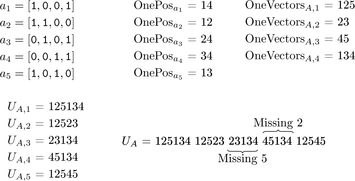
Let \(A = (a_1,\dots,a_n)\) be a sequence of \(n \geq 1\) binary vectors of dimension \(d \geq 1\). To show hardness of range distinct count queries (see 4), we construct a string over alphabet \(\{1,\dots,n\}\) consisting of \(n\) blocks such that, for each \(i\), the symbols missing from block \(i\) are exactly the indices of vectors orthogonal to \(a_i\). We start by defining the following objects (see [fig:ovreduction1] for an example showing all the objects defined below):
For each \(j \in [1 \mathinner{.\,.}d]\), we define \(\mathrm{OneVectors}_{A,j}\) to be the string containing (in increasing order) the indices \(i\) of all vectors satisfying \(a_i[j] = {\tt 1}\) (see 13).
For any vector \(x \in \{{\tt 0},{\tt 1}\}^d\), we define \(\mathrm{OnePos}_{x}\) to be the string containing (in increasing order) the indices of all coordinates \(j\) satisfying \(x[j] = {\tt 1}\) (see 14).
For every \(i \in [1 \mathinner{.\,.}n]\), we define the string \(U_{A,i}\) as follows: \[U_{A,i} := \bigodot_{j=1,\dots,k} \mathrm{OneVectors}_{A,R[j]},\] where \(R = \mathrm{OnePos}_{a_i}\) and \(k = |R|\).
Lastly, we let \(U_A := \bigodot_{i=1,\dots,n}U_{A,i}\) (see 15).
We prove that for every \(i,j \in [1 \mathinner{.\,.}n]\), the symbol \(j\) does not occur in \(U_{A,i}\) if and only if \(\left\langle a_i, a_j \right\rangle = 0\) (see 5). Therefore, \(\mathrm{distinct}_{U_{A,i}}(0, |U_{A,i}|) < n\) holds if and only if \(a_i\) is orthogonal to some vector in \(A\) (see 6). Hence, after concatenating all blocks into \(U_A\), we can use \(n\) queries \(\mathrm{distinct}_{U_A}(\cdot, \cdot)\) (4) to solve the orthogonal vectors problem on \(A\).
We demonstrate this reduction in [fig:ovreduction1]. Here, the strings \(\mathrm{OnePos}_{a_i}\) contain the indices of all coordinates \(j\) such that \(a_i[j] = {\tt 1}\) for \(i \in [1 \mathinner{.\,.}5]\), and the strings \(\mathrm{OneVectors}_{A,j}\) contain the indices of all vectors \(a_i\) such that \(a_i[j] = {\tt 1}\) for \(j \in [1 \mathinner{.\,.}4]\). The strings \(U_{A,i}\) are defined as above (15). We observe that \(U_{A,1}\) contains all elements from \(\{1,\dots,5\}\), which matches the fact that \(a_1\) is not orthogonal to any vector in \(A\). The element \(4\) is missing from \(U_{A,2}\) (and symmetrically, \(2\) is missing from \(U_{A,4}\)). This corresponds to the fact that \(\left\langle a_2, a_4 \right\rangle = 0\). Similarly, the element \(5\) is missing from \(U_{A,3}\) (and \(3\) is missing from \(U_{A,5}\)), which corresponds to \(\left\langle a_3, a_5 \right\rangle = 0\). Thus, in this example, the only pairs of orthogonal vectors are \((a_2,a_4)\) and \((a_3,a_5)\).
The string \(U_A\) can be generated by a grammar \(G\) of size \(\mathcal{O}(nd)\) that can also be constructed in \(\mathcal{O}(nd)\) time (see 15). Thus, if we can answer a batch of \(n\) queries \(\mathrm{distinct}_{U_A}(\cdot, \cdot)\) with average time \(\mathcal{O}(|G|^{1-\epsilon} \log^{\mathcal{O}(1)} N)\) per query (where \(N\) is the length of the input text), then we can solve the Orthogonal Vectors problem in sub-quadratic time (see [th:hardness-of-range-distinct-count]).
The hardness for range mode frequency queries (see 5) follows an analogous structure. We replace each string \(\mathrm{OneVectors}_{A,j}\) with its complement: we let \(\mathrm{ZeroVectors}_{A,j}\) be the string containing (in increasing order) the indices of all vectors \(a_i\) such that \(a_i[j] = {\tt 0}\) (see 16). We then define the corresponding blocks \(W_{A,i}\) (see 17). We show that symbol \(j\) appears in \(W_{A,i}\) less than \(|\mathrm{OnePos}_{a_i}|\) times if and only if \(\left\langle a_i, a_j \right\rangle \neq 0\). Thus, the maximum frequency in \(W_{A,i}\) is at least \(|\mathrm{OnePos}_{a_i}|\) if and only if \(a_i\) is orthogonal to some vector in \(A\). Proceeding as above, we obtain hardness of answering a batch of range mode frequency queries over substrings of grammar-compressed texts (see [th:hardness-of-range-mode-freq]).
3 Preliminaries↩︎
3.1 Basic Definitions↩︎
3.1.1 Strings↩︎
A string is a finite sequence of characters drawn from a given alphabet \(\Sigma\). The length of a string \(S\) is denoted by \(|S|\). For \(i \in [1 \mathinner{.\,.}|S|]\),5 the \(i\)th leftmost character of \(S\) is denoted \(S[i]\). A substring of \(S\) is any string of the form \(S[i \mathinner{.\,.}j) = S[i]S[i{+}1]\cdots S[j{-}1]\) for some \(1 \leq i \leq j \leq |S|{+}1\). Substrings of the forms \(S[1 \mathinner{.\,.}j)\) and \(S[i \mathinner{.\,.}|S|{+}1)\) are called prefixes and suffixes, respectively. The concatenation of two strings \(S_1\) and \(S_2\), namely the string \(S_1[1]\cdots S_1[|S_1|]S_2[1]\cdots S_2[|S_2|]\), is denoted by \(S_1S_2\) or \(S_1 \cdot S_2\). For \(k \in \mathbb{Z}_{\ge 0}\), we define \(S^k = \bigodot_{i=1}^k S\) as the concatenation of \(k\) copies of \(S\); by convention, \(S^0 = \varepsilon\) denotes the empty string.
3.1.2 Matrices and Vectors↩︎
A matrix \(A \in \{{\tt 0},{\tt 1}\}^{n \times m}\) is a two-dimensional array with \(n\) rows and \(m\) columns. The entry at the intersection of row \(i\) and column \(j\) is denoted as \(A[i,j]\) for every \((i,j) \in [1 \mathinner{.\,.}n] \times [1 \mathinner{.\,.}m]\). All matrix products used in this paper are over the Boolean semiring, i.e., for \(A,B \in \{{\tt 0},{\tt 1}\}^{n \times n}\), we define \(C=AB\) as \(C[i,j] = \bigvee_{k=1}^{n} A[i,k] \wedge B[k,j]\) for each \(i,j \in [1 \mathinner{.\,.}n]\).
A binary vector \(v\) of dimension \(d\) is an element of \(\{{\tt 0},{\tt 1}\}^{d}\). The \(i\)th coordinate of \(v\) is denoted as \(v[i]\). For two vectors \(u,v\) of dimension \(d\), we denote their dot product by \(\left\langle u, v \right\rangle = \sum_{i=1}^d u[i] \cdot v[i]\). We say two vectors \(u\) and \(v\) are orthogonal if \(\left\langle u, v \right\rangle = 0\).
3.2 Frequency-Based Queries↩︎
3.2.1 Symbol Occurrence and Rank Queries↩︎
Definition 1 (Symbol occurrence). Let \(T \in \Sigma^{n}\). For every \(b, e \in [0 \mathinner{.\,.}n]\) and every \(c \in \Sigma\), we define \[\mathrm{occurs}_{T}(b,e,c) := \begin{cases} 1 & \text{if there exists } j \in (b \mathinner{.\,.}e] \text{ such that }T[j] = c,\\ 0 & \text{otherwise}. \end{cases}\]
Example 1. For \(T = \texttt{acaaba}\) it holds \(\mathrm{occurs}_{T}(1,4,\texttt{a}) = 1\) and \(\mathrm{occurs}_{T}(1,4,\texttt{b}) = 0\).
Definition 2 (Rank). Let \(T \in \Sigma^{n}\). For every \(b, e \in [0 \mathinner{.\,.}n]\) and every \(c \in \Sigma\), we define \[\mathrm{rank}_{T}(b,e,c) := |\{i \in (b \mathinner{.\,.}e] : T[i] = c\}|.\] For every \(j \in [0 \mathinner{.\,.}n]\) and every \(c \in \Sigma\), we also define \[\mathrm{rank}_{T}(j,c) := \mathrm{rank}_{T}(0,j,c) = |\{i \in (0 \mathinner{.\,.}j] : T[i] = c\}|.\]
Example 2. For \(T = \texttt{acaaba}\), it holds \(\mathrm{rank}_{T}(5,\texttt{a}) = 3\) and \(\mathrm{rank}_{T}(2,5,\texttt{a}) = 2\).
Remark 1. To distinguish between the two types of rank queries in 2, by a two-sided rank query, we mean the computation of \(\mathrm{rank}_{T}(b,e,c)\), and by one-sided rank query, we refer to the computation of \(\mathrm{rank}_{T}(j,c)\). Note that, for every \(T \in \Sigma^{n}\), \(c \in \Sigma\), and \(b, e \in [0 \mathinner{.\,.}n]\) such that \(b \leq e\), it holds \(\mathrm{rank}_{T}(b,e,c) = \mathrm{rank}_{T}(e,c) - \mathrm{rank}_{T}(b,c)\).
Definition 3 (Additive rank approximation). Let \(T \in \Sigma^{n}\), \(c \in \Sigma\), and \(b, e \in [0 \mathinner{.\,.}n]\). Let \(k \in \mathbb{Z}_{\geq 1}\). We say that \(x \in \mathbb{Z}\) is a \(k\)-additive approximation of \(\mathrm{rank}_{T}(b,e,c)\) if it holds \[\mathrm{rank}_{T}(b,e,c) - k < x < \mathrm{rank}_{T}(b,e,c) + k.\]
3.2.2 Range Distinct Count Queries↩︎
Definition 4 (Range distinct count). Let \(T \in \Sigma^{n}\). For any \(b, e \in [0 \mathinner{.\,.}n]\), we define \[\mathrm{distinct}_{T}(b, e) := |\{T[i] : i \in (b \mathinner{.\,.}e]\}|.\]
Example 3. For \(T = \texttt{acaaba}\), it holds \(\mathrm{distinct}_{T}(0, 4) = 2\) and \(\mathrm{distinct}_{T}(1, 5) = 3\).
3.2.3 Range Mode Frequency Queries↩︎
Definition 5 (Range mode frequency). Let \(T \in \Sigma^{n}\). For every \(b, e \in [0 \mathinner{.\,.}n]\), we define \(\mathrm{mode-freq}_{T}(b,e)\) as the frequency of the most common element in \(T(b \mathinner{.\,.}e]\), i.e., \[\mathrm{mode-freq}_{T}(b,e) := \max_{c \in \Sigma} \mathrm{rank}_{T}(b,e,c)\] (see 2).
Example 4. For \(T = \texttt{acaaba}\) it holds \(\mathrm{mode-freq}_{T}(0,4) = 3\) and \(\mathrm{mode-freq}_{T}(3,6) = 2\).
3.3 Compressed Representations↩︎
3.3.1 Grammar Compression↩︎
A context-free grammar (CFG) is a tuple \(G = (V, \Sigma, R, S)\) such that \(V \cap \Sigma = \emptyset\) and
\(V\) is a finite nonempty set of nonterminals or variables,
\(\Sigma\) is a finite nonempty set of terminal symbols,
\(R \subseteq V \times (V \cup \Sigma)^*\) is a set of productions or rules, and
\(S \in V\) is the special starting nonterminal.
We say that \(u \in (V \cup \Sigma)^{*}\) derives \(v\), and write \(u \Rightarrow^* v\), if \(v\) can be obtained from \(u\) by repeatedly replacing nonterminals according to the rule set \(R\). We then denote \(L(G) := \{w \in \Sigma^* \mid S \Rightarrow^* w\}\).
By a straight-line grammar (SLG) we mean a CFG \(G = (V,\Sigma,R,S)\) such that:
there exists an ordering \((N_1, \dots, N_{|V|})\) of all elements in \(V\) such that, for every \((N,\gamma) \in R\), letting \(i \in [1 \mathinner{.\,.}|V|]\) be such that \(N = N_i\), it holds \(\gamma \in (\{N_{i+1}, \dots, N_{|V|}\} \cup \Sigma)^{*}\), and
for every nonterminal \(N \in V\), there exists exactly one \(\gamma \in (V \cup \Sigma)^{*}\) such that \((N,\gamma) \in R\).
The unique string \(\gamma \in (V \cup \Sigma)^{*}\) such that \((N,\gamma) \in R\) is called the definition or right-hand side of nonterminal \(N\) and is denoted \(\mathrm{rhs}_{G}(N)\). Note that in an SLG, for every \(\alpha \in (V \cup \Sigma)^{*}\), there exists exactly one string \(\gamma \in \Sigma^{*}\) satisfying \(\alpha \Rightarrow^{*} \gamma\). Such \(\gamma\) is called the expansion of \(\alpha\) and is denoted \(\mathrm{exp}_{G}(\alpha)\). In particular, in an SLG, we have \(|L(G)| = 1\). We define the size of an SLG as \(|G| = \sum_{N \in V}\max(|\mathrm{rhs}_{G}(N)|, 1)\).
An SLG in which, for every \(N \in V\), it holds \(\mathrm{rhs}_{G}(N) = XY\), where \(X,Y \in V\), or \(\mathrm{rhs}_{G}(N) = a\), where \(a \in \Sigma\), is called a straight-line program (SLP).
Observation 2. Every SLG \(G = (V, \Sigma, R, S)\) satisfying \(L(G) \neq \{\varepsilon\}\) can be transformed in \(\mathcal{O}(|G|)\) time into an SLP \(G' = (V', \Sigma, R', S')\) satisfying \(|G'| = \Theta(|G|)\) and \(L(G') = L(G)\).
Observation 3. If \(G\) is an SLP such that \(L(G) = \{T\}\), where \(|T| = n\), then \(|G| = \Omega(\log n)\).
Lemma 1 ([30]). Given any SLP \(G = (V, \Sigma, R, S)\) representing a string \(T \in \Sigma^{n}\), we can in \(\mathcal{O}(|G|)\) time construct an SLP \(G' = (V', \Sigma, R', S')\) of height \(\mathcal{O}(\log n)\) that represents the same string \(T\).
3.3.2 Lempel–Ziv (LZ78) Compression↩︎
Definition 6 (Lempel–Ziv (LZ78) factorization [60]). The LZ78 factorization of a string \(T\) is a factorization \(T = f_1 f_2 \cdots f_k\) defined such that, letting \(f_0 = \varepsilon\), for every \(i \in [1 \mathinner{.\,.}k]\), after \(f_1\cdots f_{i-1}\) has been parsed, \(f_i\) is the longest prefix of the remaining suffix \(f_i f_{i+1} \cdots f_k\) such that there exists \(j \in [0 \mathinner{.\,.}i)\) satisfying \(f_i = f_j \cdot c\) for some symbol \(c\). The elements \(f_i\) of the factorization (where \(i \geq 1\)) are called phrases. We denote the number of phrases in the LZ78 factorization of \(T\) by \(z_{78}(T)\) (i.e., \(k = z_{78}(T)\)).
Definition 7 (Lempel–Ziv (LZ78) representation). Let \(T = f_1 f_2 \cdots f_k\) be the LZ78 factorization of \(T\) (6), and let \(f_0 = \varepsilon\). The LZ78 representation of \(T\) is a sequence of pairs \(((p_1,c_1), \dots, (p_k,c_k))\) such that, for every \(i \in [1 \mathinner{.\,.}k]\), it holds \(p_i \in [0 \mathinner{.\,.}i)\) and \(f_{i} = f_{p_i} \cdot c_i\).
Remark 4. Observe that if \(T = f_1 f_2 \cdots f_k\) is the LZ78 factorization of \(T\), then all phrases \(f_1, \dots, f_{k-1}\) are distinct. Consequently, the LZ78 representation (7) of \(T\) is unique.
Remark 5. Note that if \(T \in [0 \mathinner{.\,.}\sigma)^{n}\) for some \(\sigma \in \mathbb{Z}_{\geq 1}\), then the LZ78 representation of \(T\) (7) encodes \(T\) using \(\mathcal{O}(z_{78}(T) \cdot (\log z_{78}(T) + \log \sigma)) = \mathcal{O}(z_{78}(T) \cdot (\log n + \log \sigma))\) bits of space.
Example 5. The LZ78 factorization (6) of the string \(T = \texttt{010212020}\) is \(T = \texttt{0} \cdot \texttt{1} \cdot \texttt{02} \cdot \texttt{12} \cdot \texttt{020}\) with \(z_{78}(T) = 5\) phrases, and the LZ78 representation (7) of \(T\) is: \(( (0,\texttt{0}), (0,\texttt{1}), (1,\texttt{2}), (2,\texttt{2}), (3,\texttt{0}) )\).
3.4 Hardness Assumptions↩︎
3.4.1 Boolean Matrix Multiplication (BMM)↩︎
The first problem we use as the basis of our hardness arguments is the Boolean Matrix Multiplication problem.
Two matrices \(A,B \in \{{\tt 0},{\tt 1}\}^{n \times n}\).
The matrix \(C = AB\), where \(C[i,j] = \bigvee_{k=1}^{n} A[i,k] \wedge B[k,j]\) for every \(i,j \in [1 \mathinner{.\,.}n]\).
The state-of-the-art for the above problem is summarized below, and currently no algorithm is known that solves this problem in \(\mathcal{O}(n^2 \log^{\mathcal{O}(1)} n)\) time.
Theorem 6 ([57]). Given any two Boolean matrices \(A, B \in \{{\tt 0},{\tt 1}\}^{n \times n}\), we can compute their product in \(\mathcal{O}(n^{2.371339})\) time.
3.4.2 Orthogonal Vectors (OV)↩︎
The second problem we use as a basis for our hardness results is the Orthogonal Vectors problem, one of the most widely used tools in fine-grained complexity theory (see, e.g., [65] and references therein for a recent discussion).
A set of vectors \(A \subseteq \{{\tt 0},{\tt 1}\}^d\) with \(|A| = n\).
Determine whether there exist \(x,y \in A\) such that \(\left\langle x, y \right\rangle = \sum_{i=1}^{d} x[i] \cdot y[i] = 0\).
Conjecture 7 (Orthogonal Vectors Conjecture). For every constant \(\epsilon > 0\), there exists a constant \(c \geq 1\) such that OV cannot be solved in \(\mathcal{O}(n^{2-\epsilon})\) time on instances with \(d = c\log n\).
3.5 Model of Computation↩︎
We use the standard word RAM model of computation [66] with \(w\)-bit machine words, where \(w = \Theta(\log n)\), and all standard bitwise and arithmetic operations take \(\mathcal{O}(1)\) time. Unless explicitly stated otherwise, we measure space complexity in machine words.
4 Reductions from Boolean Matrix Multiplication↩︎
4.1 Hardness of Symbol Occurrence Queries on Grammars↩︎
Definition 8 (String with positions of all \({\tt 1}\)s in a given row). Let \(A \in \{{\tt 0},{\tt 1}\}^{n \times n}\), where \(n \geq 1\). For every \(i \in [1 \mathinner{.\,.}n]\), by \(\mathrm{RowOnes}_{A,i}\), we denote a string containing in increasing order the positions of all ones in the \(i\)th row of \(A\), i.e., \(\mathrm{RowOnes}_{A,i} \in \{1, \dots, n\}^{*}\) is such that, letting \(k = |\mathrm{RowOnes}_{A,i}|\), it holds
if \(k > 0\), then \(\mathrm{RowOnes}_{A,i}[1] < \dots < \mathrm{RowOnes}_{A,i}[k]\), and
\(\{\mathrm{RowOnes}_{A,i}[t]\}_{t \in [1 \mathinner{.\,.}k]} = \{j \in [1 \mathinner{.\,.}n] : A[i,j] = {\tt 1}\}\).
Definition 9 (Grammar-compressible encoding of the product \(AB\) as a string). Let \(A, B \in \{{\tt 0},{\tt 1}\}^{n \times n}\), where \(n \geq 1\). For every \(i \in [1 \mathinner{.\,.}n]\), we denote \[T_{A,B,i} := \textstyle\bigodot_{t=1,\dots,k} \mathrm{RowOnes}_{B,R[t]},\] where \(R = \mathrm{RowOnes}_{A,i}\) (8) and \(k = |R|\). We then let \[T_{A,B} := \textstyle\bigodot_{i=1,\dots,n} T_{A,B,i}.\]
Observation 8. For every \(A,B \in \{{\tt 0},{\tt 1}\}^{n \times n}\), the string \(T_{A,B}\) (9) satisfies \(|T_{A,B}| \leq n^3\).
Proof. For all \(i \in [1 \mathinner{.\,.}n]\), it holds \(|\mathrm{RowOnes}_{A,i}| \leq n\) and \(|\mathrm{RowOnes}_{B,i}| \leq n\). Since \(T_{A,B,i}\) is a concatenation of at most \(n\) strings each of which has length at most \(n\), we thus have \(|T_{A,B,i}| \leq n^2\) for all \(i \in [1 \mathinner{.\,.}n]\). Consequently, \(|T_{A,B}| \leq n^3\). ◻
Lemma 2. Let \(A,B \in \{{\tt 0},{\tt 1}\}^{n \times n}\). For every \(i,j \in [1 \mathinner{.\,.}n]\), the following conditions are equivalent:
Symbol \(j\) occurs in the string \(T_{A,B,i}\) (see 9),
It holds \((AB)[i,j] = {\tt 1}\) (where \(AB\) denotes the Boolean matrix multiplication).
Proof. ([lm:sym-occ-and-mat-mul-equivalence-it-1]) \(\Rightarrow\) ([lm:sym-occ-and-mat-mul-equivalence-it-2]) Assume that symbol \(j\) occurs in the string \(T_{A,B,i}\). Denote \(R = \mathrm{RowOnes}_{A,i}\) and \(k = |R|\). By 9, the assumption that \(j\) occurs in \(T_{A,B,i}\) implies that there exists \(t \in [1 \mathinner{.\,.}k]\) such that \(j\) occurs in the string \(\mathrm{RowOnes}_{B,R[t]}\). By definition of \(\mathrm{RowOnes}_{B,R[t]}\), this implies that \(B[R[t],j] = {\tt 1}\). On the other hand, by definition of \(R = \mathrm{RowOnes}_{A,i}\), we have \(A[i,R[t]] = {\tt 1}\). Consequently, \(A[i,R[t]] \wedge B[R[t],j] = {\tt 1}\). Hence, \((AB)[i,j] = {\tt 1}\).
([lm:sym-occ-and-mat-mul-equivalence-it-2]) \(\Rightarrow\) ([lm:sym-occ-and-mat-mul-equivalence-it-1]) Let us now assume that \((AB)[i,j] = {\tt 1}\). This implies that there exists \(p \in [1 \mathinner{.\,.}n]\) such that \(A[i,p] = {\tt 1}\) and \(B[p,j] = {\tt 1}\). Denote again \(R = \mathrm{RowOnes}_{A,i}\) and \(k = |R|\). On the one hand, \(A[i,p] = {\tt 1}\) implies that \(p\) occurs in \(R\), i.e., there exists \(t \in [1 \mathinner{.\,.}k]\) such that \(p = R[t]\). On the other hand, by \(B[p,j] = {\tt 1}\), we obtain that \(j\) occurs in \(\mathrm{RowOnes}_{B,p} = \mathrm{RowOnes}_{B,R[t]}\). We have thus proved that there exists \(t \in [1 \mathinner{.\,.}k]\) such that \(j\) occurs in \(\mathrm{RowOnes}_{B,R[t]}\). Since \(\mathrm{RowOnes}_{B,R[t]}\) is a substring of \(T_{A,B,i}\), we thus obtain that \(j\) occurs in \(T_{A,B,i}\). ◻
Proposition 9. Given any \(A, B \in \{{\tt 0},{\tt 1}\}^{n \times n}\), we can in \(\mathcal{O}(n^2)\) time construct an SLG \(G = (V, \Sigma, R, S)\) such that \(\Sigma = \{1, \dots, n\}\) and \(L(G) = \{T_{A,B}\}\) (9).
Proof. Let \(V = \{X_1, \dots, X_n, Y_1, \dots, Y_n, S\}\). For every \(i \in [1 \mathinner{.\,.}n]\), we set \(\mathrm{rhs}_{G}(X_i) = \mathrm{RowOnes}_{B,i} \in \{1, \dots, n\}^{*}\) (8). For every \(i \in [1 \mathinner{.\,.}n]\), letting \(R = \mathrm{RowOnes}_{A,i}\) and \(k = |R|\), we set \(\mathrm{rhs}_{G}(Y_i) = X_{R[1]} \cdot X_{R[2]} \cdots X_{R[k]}\), with the right-hand side interpreted as \(\varepsilon\) if \(k=0\). Finally, we set \(\mathrm{rhs}_{G}(S) = Y_1 \cdot Y_2 \cdots Y_n\).
To construct \(G\), we proceed as follows:
First, in \(\mathcal{O}(n^2)\) time we compute the strings \(\mathrm{RowOnes}_{A,i}\) and \(\mathrm{RowOnes}_{B,i}\) for all \(i \in [1 \mathinner{.\,.}n]\).
Given the above strings, the construction of \(\mathrm{rhs}_{G}(N)\) for all \(N \in V\) takes \(\mathcal{O}(n^2)\) time.
In total, the construction takes \(\mathcal{O}(n^2)\) time.
To show that \(L(G) = \{T_{A,B}\}\), it suffices to observe that, for every \(i \in [1 \mathinner{.\,.}n]\), it holds \(\mathrm{exp}_{G}(Y_i) = T_{A,B,i}\) (see 9). Thus, \(L(G) = \{\mathrm{exp}_{G}(S)\} = \{\bigodot_{i=1,\dots,n}\mathrm{exp}_{G}(Y_i)\} = \{T_{A,B}\}\). ◻
Proof. Let \(A,B \in \{{\tt 0},{\tt 1}\}^{n \times n}\) be two given Boolean matrices. The algorithm to compute the Boolean matrix product \(AB\) proceeds as follows:
In this step, we compute an array \(A_{\rm sum}[0 \mathinner{.\,.}n]\) defined such that \(A_{\rm sum}[0] = 0\) and, for every \(i \in [1 \mathinner{.\,.}n]\), \(A_{\rm sum}[i] = \sum_{j=1}^{i} |T_{A,B,j}|\) (see 9). We begin by computing an array \(A_{\rm len}[1 \mathinner{.\,.}n]\) defined by \(A_{\rm len}[i] = |T_{A,B,i}|\). To this end, we first in \(\mathcal{O}(n^2)\) time compute the strings \(\mathrm{RowOnes}_{A,i}\) and \(\mathrm{RowOnes}_{B,i}\) (see 8) for all \(i \in [1 \mathinner{.\,.}n]\). Using these strings, we can then compute \(|T_{A,B,i}|\) for any \(i \in [1 \mathinner{.\,.}n]\) in \(\mathcal{O}(n)\) time (see 9). In total, computing \(A_{\rm len}[1 \mathinner{.\,.}n]\) takes \(\mathcal{O}(n^2)\) time. Using \(A_{\rm len}\), we then easily obtain \(A_{\rm sum}\) in \(\mathcal{O}(n)\) time. In total, construction of \(A_{\rm sum}[0 \mathinner{.\,.}n]\) takes \(\mathcal{O}(n^2)\) time. Observe that by 9, for any \(i \in [1 \mathinner{.\,.}n]\), it holds \[T_{A,B}(A_{\rm sum}[i-1] \mathinner{.\,.}A_{\rm sum}[i]] = T_{A,B,i}.\] If \(A_{\rm sum}[n] = 0\), then \(T_{A,B,i}\) is empty for every \(i \in [1 \mathinner{.\,.}n]\). By 2, the output matrix \(AB\) then consists only of zeros. In this case, we return the \(n \times n\) zero matrix in \(\mathcal{O}(n^2)\) time and conclude the algorithm. Henceforth, assume that \(A_{\rm sum}[n] > 0\).
Using 9, in \(\mathcal{O}(n^2)\) time we construct an SLG \(G = (V, \Sigma, R, S)\) such that \(\Sigma = \{1, \dots, \sigma\}\) (where \(\sigma = n\)) and \(L(G) = \{T\}\), where \(T = T_{A,B}\) (9). Note that the upper bound on the runtime of 9 implies that \(|G| = \mathcal{O}(n^2)\). Denote \(N = |T|\) and recall that \(N \leq n^3\) (8). Observe also that we then have \(\sigma = n = \Omega(N^{1/3})\).
In this step, we compute the product \(AB\). By 2, computing \((AB)[i,j]\) for any given \(i,j \in [1 \mathinner{.\,.}n]\) can be done using a single symbol occurrence query. More precisely, by 2 and the above discussion, it holds (see 1) \[\begin{align} (AB)[i,j] &= \mathrm{occurs}_{T_{A,B,i}}(0,|T_{A,B,i}|,j)\\ &= \mathrm{occurs}_{T_{A,B}}(A_{\rm sum}[i-1],A_{\rm sum}[i],j)\\ &= \mathrm{occurs}_{T}(A_{\rm sum}[i-1],A_{\rm sum}[i],j). \end{align}\] Using the array \(A_{\rm sum}\), in \(\mathcal{O}(n^2)\) time we prepare the arguments for a batch of \(m = n^2\) symbol occurrence queries on \(T\). Using the algorithm from the claim, we then answer all the queries (and hence compute the product \(AB\)) in \(\mathcal{O}((|G| + m) \log^{\mathcal{O}(1)} N) = \mathcal{O}(n^2 \log^{\mathcal{O}(1)} (n^3)) = \mathcal{O}(n^2 \log^{\mathcal{O}(1)} n)\) time.
In total, the algorithm takes \(\mathcal{O}(n^2 \log^{\mathcal{O}(1)} n)\) time. ◻
4.2 Hardness of Symbol Occurrence Queries on LZ78↩︎
Definition 10 (Prefix concatenation string). For any string \(T \in \Sigma^{n}\), we denote \[\mathrm{prefixes}(T) := \textstyle\bigodot_{i=1,\dots,n} T[1 \mathinner{.\,.}i] \in \Sigma^{n(n+1)/2}.\]
Lemma 3. Let \(m, k \in \mathbb{Z}_{\geq 1}\). Let \((S_i)_{i \in [1 \mathinner{.\,.}m]}\) be a sequence of strings over alphabet \(\Sigma = \{1, \ldots, \sigma\}\). Let \(\text{\normalfont \texttt{\$}}_1, \ldots, \text{\normalfont \texttt{\$}}_m, \text{\normalfont \texttt{\#}}_1, \ldots, \text{\normalfont \texttt{\#}}_k\) be pairwise distinct symbols that do not belong to \(\Sigma\). Denote \(\hat{\Sigma} = \Sigma \cup \{\text{\normalfont \texttt{\$}}_1, \text{\normalfont \texttt{\$}}_2, \ldots, \text{\normalfont \texttt{\$}}_m \} \cup \{\text{\normalfont \texttt{\#}}_1, \text{\normalfont \texttt{\#}}_2, \ldots, \text{\normalfont \texttt{\#}}_k\}\). For every \(i \in [1 \mathinner{.\,.}k]\), let \(n_i \in \mathbb{Z}_{\geq 0}\) and \((p_{i,j})_{j \in [1 \mathinner{.\,.}n_i]}\) be a possibly empty sequence of integers such that, whenever \(n_i > 0\), \(1 \leq p_{i,1} < p_{i,2} < \cdots < p_{i,n_i} \leq m\). For every \(i \in [1 \mathinner{.\,.}k]\), we define the following string (parentheses added for clarity): \[T_{i} := \textstyle\bigodot_{j=1,\ldots,n_i} \Big(\text{\normalfont \texttt{\$}}_{p_{i,j}} \cdot S_{p_{i,j}} \cdot \text{\normalfont \texttt{\#}}_{i}\Big) \in \hat{\Sigma}^{*}.\] We also define (see 10): \[T := \Big(\textstyle\bigodot_{i=1,\ldots,m} \mathrm{prefixes}(\text{\normalfont \texttt{\$}}_i \cdot S_i)\Big) \cdot \Big(\bigodot_{i=1,\ldots,k} T_{i}\Big) \in \hat{\Sigma}^{*}.\] Then, the LZ78 factorization (6) of \(T\) is (with empty terms omitted): \[\begin{align} T ={}\;& \begin{array}[t]{@{}l c l c l c l c l c@{}} \text{\normalfont \texttt{\$}}_1 & \odot & \text{\normalfont \texttt{\$}}_1 S_1[1] & \odot & \text{\normalfont \texttt{\$}}_1 S_1[1\mathinner{.\,.}2] & \odot & \text{\normalfont \texttt{\$}}_1 S_1[1\mathinner{.\,.}3] & \cdots & \text{\normalfont \texttt{\$}}_1 S_1[1\mathinner{.\,.}|S_1|] & \odot \\ \text{\normalfont \texttt{\$}}_2 & \odot & \text{\normalfont \texttt{\$}}_2 S_2[1] & \odot & \text{\normalfont \texttt{\$}}_2 S_2[1\mathinner{.\,.}2] & \odot & \text{\normalfont \texttt{\$}}_2 S_2[1\mathinner{.\,.}3] & \cdots & \text{\normalfont \texttt{\$}}_2 S_2[1\mathinner{.\,.}|S_2|] & \odot \\ \vdots & & \vdots & & \vdots & & \vdots & & \vdots & \\ \text{\normalfont \texttt{\$}}_m & \odot & \text{\normalfont \texttt{\$}}_m S_m[1] & \odot & \text{\normalfont \texttt{\$}}_m S_m[1\mathinner{.\,.}2] & \odot & \text{\normalfont \texttt{\$}}_m S_m[1\mathinner{.\,.}3] & \cdots & \text{\normalfont \texttt{\$}}_m S_m[1\mathinner{.\,.}|S_m|] & \odot \end{array} \\[0.6ex] &\begin{array}[t]{@{}l c l c l c l c@{}} \text{\normalfont \texttt{\$}}_{p_{1,1}} S_{p_{1,1}} \text{\normalfont \texttt{\#}}_{1} & \odot & \text{\normalfont \texttt{\$}}_{p_{1,2}} S_{p_{1,2}} \text{\normalfont \texttt{\#}}_{1} & \odot & \text{\normalfont \texttt{\$}}_{p_{1,3}} S_{p_{1,3}} \text{\normalfont \texttt{\#}}_{1} & \cdots & \text{\normalfont \texttt{\$}}_{p_{1,n_1}} S_{p_{1,n_1}} \text{\normalfont \texttt{\#}}_{1} & \odot \\ \text{\normalfont \texttt{\$}}_{p_{2,1}} S_{p_{2,1}} \text{\normalfont \texttt{\#}}_{2} & \odot & \text{\normalfont \texttt{\$}}_{p_{2,2}} S_{p_{2,2}} \text{\normalfont \texttt{\#}}_{2} & \odot & \text{\normalfont \texttt{\$}}_{p_{2,3}} S_{p_{2,3}} \text{\normalfont \texttt{\#}}_{2} & \cdots & \text{\normalfont \texttt{\$}}_{p_{2,n_2}} S_{p_{2,n_2}} \text{\normalfont \texttt{\#}}_{2} & \odot \\ \vdots & & \vdots & & \vdots & & \vdots & \\ \text{\normalfont \texttt{\$}}_{p_{k,1}} S_{p_{k,1}} \text{\normalfont \texttt{\#}}_{k} & \odot & \text{\normalfont \texttt{\$}}_{p_{k,2}} S_{p_{k,2}} \text{\normalfont \texttt{\#}}_{k} & \odot & \text{\normalfont \texttt{\$}}_{p_{k,3}} S_{p_{k,3}} \text{\normalfont \texttt{\#}}_{k} & \cdots & \text{\normalfont \texttt{\$}}_{p_{k,n_k}} S_{p_{k,n_k}} \text{\normalfont \texttt{\#}}_{k}. & \end{array} \end{align}\] In particular, \(z_{78}(T) = m + \sum_{j=1}^{m} |S_j| + \sum_{i=1}^{k} n_i\). Moreover, letting \((a_i)_{i \in [0 \mathinner{.\,.}m]}\) be a sequence defined such that, for any \(i \in [0 \mathinner{.\,.}m]\), \(a_i = \sum_{j=1}^{i} |S_j|\), in the LZ78 representation (7) of \(T\):
a phrase \(\text{\normalfont \texttt{\$}}_i\), where \(i \in [1 \mathinner{.\,.}m]\), is encoded as \((0,\text{\normalfont \texttt{\$}}_i)\),
a phrase \(\text{\normalfont \texttt{\$}}_i \cdot S_i[1 \mathinner{.\,.}j]\), where \(i \in [1 \mathinner{.\,.}m]\) and \(j \in [1 \mathinner{.\,.}|S_i|]\), is encoded as \((a_{i-1}+(i-1)+j, S_i[j])\),
a phrase \(\text{\normalfont \texttt{\$}}_{p_{i,j}} \cdot S_{p_{i,j}} \cdot \text{\normalfont \texttt{\#}}_i\), where \(i \in [1 \mathinner{.\,.}k]\) and \(j \in [1 \mathinner{.\,.}n_i]\), is encoded as \((a_{p_{i,j}}+p_{i,j},\text{\normalfont \texttt{\#}}_i)\).
Proof. For each \(i \in [1 \mathinner{.\,.}m]\), let \(X_i := \text{\normalfont \texttt{\$}}_i \cdot S_i\). We first prove by induction on \(i\) that, for every \(i \in [1 \mathinner{.\,.}m]\), the first \(i+a_i\) phrases in the LZ78 factorization of \(T\) are exactly the phrases \(X_1[1], X_1[1 \mathinner{.\,.}2], \ldots, X_1[1 \mathinner{.\,.}|X_1|], \ldots, X_i[1], X_i[1 \mathinner{.\,.}2], \ldots, X_i[1 \mathinner{.\,.}|X_i|]\), i.e., \(\text{\normalfont \texttt{\$}}_1, \text{\normalfont \texttt{\$}}_1S_1[1], \ldots, \text{\normalfont \texttt{\$}}_1S_1, \ldots, \text{\normalfont \texttt{\$}}_i, \text{\normalfont \texttt{\$}}_iS_i[1], \ldots, \text{\normalfont \texttt{\$}}_iS_i\).
For the base case \(i=1\), note that the prefix of \(T\) corresponding to \(\mathrm{prefixes}(X_1)\) is exactly \(X_1[1] \cdot X_1[1 \mathinner{.\,.}2] \cdots X_1[1 \mathinner{.\,.}|X_1|]\). The first phrase is therefore \(X_1[1]=\text{\normalfont \texttt{\$}}_1\), since \(\text{\normalfont \texttt{\$}}_1\) has not occurred earlier. After this, the unread suffix again starts with \(\text{\normalfont \texttt{\$}}_1\). More generally, whenever the phrases \(X_1[1], X_1[1 \mathinner{.\,.} 2], \ldots, X_1[1 \mathinner{.\,.}r]\) have already been produced, the next unread position starts with \(X_1[1 \mathinner{.\,.}r+1]\); this string is obtained by extending the earlier phrase \(X_1[1 \mathinner{.\,.}r]\) by one symbol, and no longer phrase can be chosen, because among all earlier phrases the only ones starting with \(\text{\normalfont \texttt{\$}}_1\) are precisely \(X_1[1], X_1[1 \mathinner{.\,.}2], \ldots, X_1[1 \mathinner{.\,.}r]\). Hence the phrases contributed by \(\mathrm{prefixes}(X_1)\) are exactly \(X_1[1], X_1[1 \mathinner{.\,.} 2], \ldots, X_1[1 \mathinner{.\,.}|X_1|]\).
For the induction step, assume that the claim holds for some \(i \in [1 \mathinner{.\,.}m)\), and let \(\delta := i+a_i\). Then the first \(\delta\) phrases are exactly those coming from \(\mathrm{prefixes}(X_1), \ldots, \mathrm{prefixes}(X_i)\). The next unread part of \(T\) begins with \(\mathrm{prefixes}(X_{i+1})\), namely with \(X_{i+1}[1] \cdot X_{i+1}[1 \mathinner{.\,.}2] \cdots X_{i+1}[1 \mathinner{.\,.} |X_{i+1}|]\). Since \(\text{\normalfont \texttt{\$}}_{i+1}\) does not occur in the already parsed prefix, the next phrase is \(X_{i+1}[1]=\text{\normalfont \texttt{\$}}_{i+1}\). Repeating the same argument as in the base case, after the phrases \(X_{i+1}[1], X_{i+1}[1 \mathinner{.\,.} 2], \ldots, X_{i+1}[1 \mathinner{.\,.}r]\) have been produced, the next unread suffix starts with \(X_{i+1}[1 \mathinner{.\,.}r+1]\); this is obtained by extending the previous phrase \(X_{i+1}[1 \mathinner{.\,.}r]\), and it is maximal because the only earlier phrases starting with \(\text{\normalfont \texttt{\$}}_{i+1}\) are the prefixes already created in this block. Thus the phrases contributed by \(\mathrm{prefixes}(X_{i+1})\) are exactly \(X_{i+1}[1], X_{i+1}[1 \mathinner{.\,.}2], \ldots, X_{i+1}[1 \mathinner{.\,.} |X_{i+1}|]\). This proves the induction claim.
Let \(\Delta := m+a_m\). By the above, the first \(\Delta\) phrases in the LZ78 factorization of \(T\) are exactly \(\text{\normalfont \texttt{\$}}_1, \text{\normalfont \texttt{\$}}_1S_1[1], \ldots, \text{\normalfont \texttt{\$}}_1S_1, \ldots, \text{\normalfont \texttt{\$}}_m, \text{\normalfont \texttt{\$}}_mS_m[1], \ldots, \text{\normalfont \texttt{\$}}_mS_m\), and the remaining suffix is \(\bigodot_{i=1,\ldots,k} T_i\). Consider any substring of this suffix of the form \(\text{\normalfont \texttt{\$}}_t \cdot S_t \cdot \text{\normalfont \texttt{\#}}_r\), where \(t \in [1 \mathinner{.\,.}m]\) and \(r \in [1 \mathinner{.\,.} k]\). Since \(\text{\normalfont \texttt{\$}}_tS_t\) is already one of the first \(\Delta\) phrases, the string \(\text{\normalfont \texttt{\$}}_tS_t\text{\normalfont \texttt{\#}}_r\) can be chosen as the next LZ78 phrase. It is also maximal: indeed, if a longer phrase were to start here, then there would exist an earlier phrase \(Q\) that matches a longer prefix of the unread suffix and has \(\text{\normalfont \texttt{\$}}_tS_t\text{\normalfont \texttt{\#}}_r\) as a prefix. Since every nonempty LZ78 phrase is obtained from an earlier phrase by appending one symbol, repeatedly following source phrases from \(Q\) shows that every nonempty prefix of \(Q\) is also an earlier phrase. In particular, the string \(\text{\normalfont \texttt{\$}}_tS_t\text{\normalfont \texttt{\#}}_r\) itself would have to occur earlier as a phrase. This is impossible, because \(\text{\normalfont \texttt{\#}}_r\) does not occur in the prefix \(\bigodot_{i=1,\ldots,m} \mathrm{prefixes}(\text{\normalfont \texttt{\$}}_iS_i)\), and within the suffix \(\bigodot_{i=1,\ldots,k} T_i\) each substring \(\text{\normalfont \texttt{\$}}_tS_t\text{\normalfont \texttt{\#}}_r\) appears at most once: any occurrence of \(\text{\normalfont \texttt{\$}}_tS_t\text{\normalfont \texttt{\#}}_r\) must start at an occurrence of \(\text{\normalfont \texttt{\$}}_t\), and since each \(S_u\) belongs to \(\Sigma^*\) while all symbols \(\text{\normalfont \texttt{\$}}_1,\ldots,\text{\normalfont \texttt{\$}}_m,\text{\normalfont \texttt{\#}}_1,\ldots,\text{\normalfont \texttt{\#}}_k\) lie outside \(\Sigma\), the symbol \(\text{\normalfont \texttt{\$}}_t\) can occur in the suffix only as the first symbol of one of the blocks \(\text{\normalfont \texttt{\$}}_{p_{u,v}}S_{p_{u,v}}\text{\normalfont \texttt{\#}}_u\); for fixed \(r\) this follows from the strict inequalities \(p_{r,1} < \cdots < p_{r,n_r}\), and for different values of \(r\) the last symbol differs since \(\text{\normalfont \texttt{\#}}_1,\ldots,\text{\normalfont \texttt{\#}}_k\) are distinct. Therefore each substring \(\text{\normalfont \texttt{\$}}_{p_{i,j}} S_{p_{i,j}} \text{\normalfont \texttt{\#}}_i\) forms one phrase of the LZ78 factorization of \(T\), in the stated order. This proves the claimed formula for the factorization. In particular, the number of phrases is \(\Delta + \sum_{i=1}^{k} n_i = m + \sum_{j=1}^{m} |S_j| + \sum_{i=1}^{k} n_i\).
It remains to verify the formulas for the LZ78 representation.
A phrase \(\text{\normalfont \texttt{\$}}_i\), where \(i \in [1 \mathinner{.\,.}m]\), is encoded as \((0,\text{\normalfont \texttt{\$}}_i)\) by definition.
Next, let us consider a phrase \(\text{\normalfont \texttt{\$}}_i \cdot S_i[1 \mathinner{.\,.}j]\), where \(i \in [1 \mathinner{.\,.}m]\) and \(j \in [1 \mathinner{.\,.}|S_i|]\). This is the phrase \(X_i[1 \mathinner{.\,.}j+1]\), and it is the \((a_{i-1}+(i-1)+(j+1))\)th phrase in the factorization. Its source phrase is the immediately preceding phrase \(X_i[1 \mathinner{.\,.}j]\), whose index is \(a_{i-1}+(i-1)+j\). Therefore its encoding is \((a_{i-1}+(i-1)+j, S_i[j])\).
Finally, let us consider a phrase \(\text{\normalfont \texttt{\$}}_{p_{i,j}} \cdot S_{p_{i,j}} \cdot \text{\normalfont \texttt{\#}}_i\), where \(i \in [1 \mathinner{.\,.}k]\) and \(j \in [1 \mathinner{.\,.}n_i]\). Its source is the phrase \(\text{\normalfont \texttt{\$}}_{p_{i,j}} \cdot S_{p_{i,j}}\), and by the first part of the proof that source is the \((a_{p_{i,j}} + p_{i,j})\)th phrase. Hence the encoding of \(\text{\normalfont \texttt{\$}}_{p_{i,j}} \cdot S_{p_{i,j}} \cdot \text{\normalfont \texttt{\#}}_i\) is \((a_{p_{i,j}} + p_{i,j}, \text{\normalfont \texttt{\#}}_i)\).
◻
Definition 11 (LZ78-compressible encoding of the product \(AB\) as a string). Let \(A, B \in \{{\tt 0},{\tt 1}\}^{n \times n}\), where \(n \geq 1\). For every \(i \in [1 \mathinner{.\,.}n]\), we define the string (parentheses added for clarity): \[X_{A,B,i} := \textstyle\bigodot_{t=1,\dots,k} \Big( (n+R[t]) \cdot \mathrm{RowOnes}_{B,R[t]} \cdot (2n + i) \Big) \in [1 \mathinner{.\,.}3n]^{*},\] where \(R = \mathrm{RowOnes}_{A,i}\) (8) and \(k = |R|\). We then let (see 10) \[X_{A,B} := \Big( \textstyle\bigodot_{i=1,\ldots,n} \mathrm{prefixes}((n+i) \cdot \mathrm{RowOnes}_{B,i}) \Big) \cdot \Big( \textstyle\bigodot_{i=1,\dots,n} X_{A,B,i} \Big) \in [1 \mathinner{.\,.}3n]^{*}.\]
Observation 10. For every \(A,B \in \{{\tt 0},{\tt 1}\}^{n \times n}\), the string \(X_{A,B}\) (11) satisfies \(|X_{A,B}| \leq 6n^3\).
Proof. For all \(i \in [1 \mathinner{.\,.}n]\), it holds \(|\mathrm{RowOnes}_{A,i}| \leq n\) and \(|\mathrm{RowOnes}_{B,i}| \leq n\). Thus, \(X_{A,B,i}\) is a concatenation of at most \(n\) strings each of which has length at most \(n+2\), and hence \(|X_{A,B,i}| \leq n(n+2)\) for all \(i \in [1 \mathinner{.\,.}n]\). On the other hand, by 10, for every \(i \in [1 \mathinner{.\,.}n]\), letting \(k = |\mathrm{RowOnes}_{B,i}|\), it holds \(|\mathrm{prefixes}((n+i) \cdot \mathrm{RowOnes}_{B,i})| = (k+1)(k+2)/2 \leq (n+1)(n+2)/2\). Consequently, \(|X_{A,B}| \leq n(n+1)(n+2)/2 + n^2(n+2) = \tfrac{3}{2}n^3 + \tfrac{7}{2}n^2 + n \leq 6n^3\). ◻
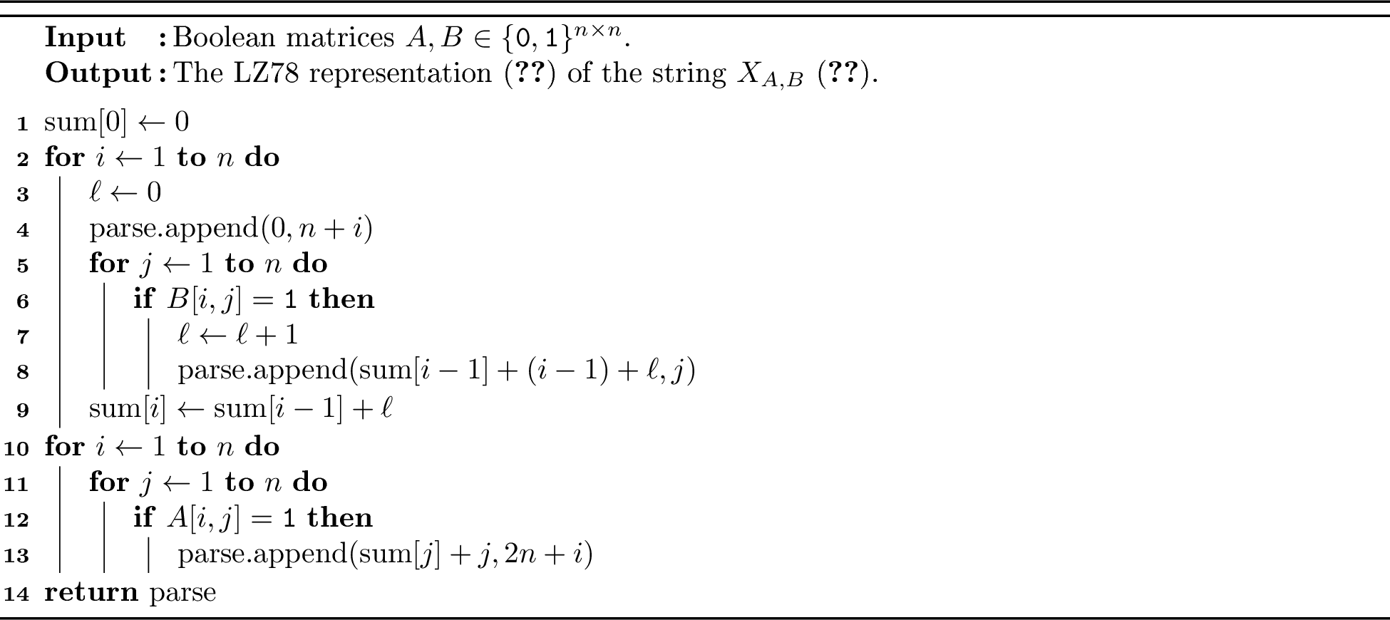
Proposition 11. Given any \(A, B \in \{{\tt 0},{\tt 1}\}^{n \times n}\), we can compute the LZ78 representation (7) of the string \(X_{A,B}\) (11) in \(\mathcal{O}(n^2)\) time.
Proof. Observe that letting \(S_i = \mathrm{RowOnes}_{B,i}\), \(n_i = |\mathrm{RowOnes}_{A,i}|\), and \((p_{i,j})_{j=1,\ldots,n_i}\) (where \(i \in [1 \mathinner{.\,.}n]\)) be the sequence of symbols in \(\mathrm{RowOnes}_{A,i}\), the string \(T\) from 3 is equal to the string \(X_{A,B}\), assuming we map symbols in the sets \(\{\text{\normalfont \texttt{\$}}_1, \dots, \text{\normalfont \texttt{\$}}_n\}\) and \(\{\text{\normalfont \texttt{\#}}_1, \dots, \text{\normalfont \texttt{\#}}_n\}\) so that for every \(i \in [1 \mathinner{.\,.}n]\), \(\text{\normalfont \texttt{\$}}_i\) (resp. \(\text{\normalfont \texttt{\#}}_i\)) is mapped to \(n + i\) (resp.\(2n + i\)). By 3, we can thus compute the LZ78 representation of \(X_{A,B}\) as follows:
In \(\mathcal{O}(n^2)\) time, we compute, for \(i \in [1 \mathinner{.\,.}n]\), the strings \(A_i = \mathrm{RowOnes}_{A,i}\) and \(B_i = \mathrm{RowOnes}_{B,i}\).
In \(\mathcal{O}(n)\) time, we compute an array \({\rm sum}[0 \mathinner{.\,.}n]\) defined such that \({\rm sum}[0] = 0\) and, for every \(i \in [1 \mathinner{.\,.}n]\), \({\rm sum}[i] = {\rm sum}[i-1] + |B_i|\).
For \(i=1,\ldots,n\), perform the following steps:
First, append the pair \((0, n+i)\) to the output LZ78 representation.
For \(j=1,\ldots,|B_i|\), append the pair \(({\rm sum}[i-1]+(i-1)+j,B_i[j])\) to the output LZ78 representation.
In total, this takes \(\mathcal{O}(n^2)\) time.
For \(i=1,\ldots,n\), scan the sequence \(A_i\) left-to-right and, for every \(j \in [1 \mathinner{.\,.}|A_i|]\), append the pair \(({\rm sum}[A_i[j]] + A_i[j], 2n + i)\) to the output LZ78 representation. In total, this takes \(\mathcal{O}(n^2)\) time.
In total, the computation takes \(\mathcal{O}(n^2)\) time. An equivalent optimized implementation, which avoids explicitly storing the strings \(A_i\) and \(B_i\), is given in 3. ◻
Proof. Let \(A,B \in \{{\tt 0},{\tt 1}\}^{n \times n}\) be two given Boolean matrices. The algorithm to compute the Boolean matrix product \(AB\) proceeds as follows:
In the first step, we compute the integer \(\Delta = \sum_{i=1}^{n} |\mathrm{prefixes}((n+i) \cdot \mathrm{RowOnes}_{B,i})|\). To this end, we first in \(\mathcal{O}(n^2)\) time compute the strings \(\mathrm{RowOnes}_{B,i}\) for all \(i \in [1 \mathinner{.\,.}n]\). Using their lengths, the computation of \(\Delta\) takes \(\mathcal{O}(n)\) time (see 10).
In the second step, we compute an array \(A_{\rm sum}[0 \mathinner{.\,.}n]\) defined such that \(A_{\rm sum}[0] = 0\) and, for every \(i \in [1 \mathinner{.\,.}n]\), \(A_{\rm sum}[i] = \sum_{j=1}^{i} |X_{A,B,j}|\) (see 11). We begin by computing an array \(A_{\rm len}[1 \mathinner{.\,.}n]\) defined by \(A_{\rm len}[i] = |X_{A,B,i}|\). To this end, we first in \(\mathcal{O}(n^2)\) time compute the strings \(\mathrm{RowOnes}_{A,i}\) and \(\mathrm{RowOnes}_{B,i}\) (see 8) for all \(i \in [1 \mathinner{.\,.}n]\). Using these strings, we can then compute \(|X_{A,B,i}|\) for any \(i \in [1 \mathinner{.\,.}n]\) in \(\mathcal{O}(n)\) time (see 11). In total, computing \(A_{\rm len}[1 \mathinner{.\,.}n]\) takes \(\mathcal{O}(n^2)\) time. Using \(A_{\rm len}\), we then easily obtain \(A_{\rm sum}\) in \(\mathcal{O}(n)\) time. In total, construction of \(A_{\rm sum}[0 \mathinner{.\,.}n]\) takes \(\mathcal{O}(n^2)\) time. Observe that by 11, for any \(i \in [1 \mathinner{.\,.}n]\), it holds \[X_{A,B}(\Delta + A_{\rm sum}[i-1] \mathinner{.\,.}\Delta + A_{\rm sum}[i]] = X_{A,B,i}.\]
Using 11, in \(\mathcal{O}(n^2)\) time we compute the LZ78 representation of the string \(T = X_{A,B}\) (11). Note that \(T\) is over alphabet \(\Sigma = \{1, \dots, \sigma\}\), where \(\sigma = 3n\). Note also that by 11 and 3, it follows that \(z_{78}(T) = n + \sum_{i=1}^{n} |\mathrm{RowOnes}_{B,i}| + \sum_{i=1}^{n} |\mathrm{RowOnes}_{A,i}| \leq n + 2n^2\). Denote \(N = |T|\) and recall that \(N \leq 6n^3\) (10). We then have \(\sigma = 3n = \Omega(N^{1/3})\).
In this step, we compute the product \(AB\). By 2, computing \((AB)[i,j]\) for any given \(i,j \in [1 \mathinner{.\,.}n]\) can be done using a single symbol occurrence query on the string \(T_{A,B,i}\) (9). More precisely, by 2, it holds \((AB)[i,j] = \mathrm{occurs}_{T_{A,B,i}}(0,|T_{A,B,i}|,j)\). On the other hand, note that by comparing 9 and 11, we immediately have that since \(j \in [1 \mathinner{.\,.}n]\), it holds \(\mathrm{occurs}_{T_{A,B,i}}(0,|T_{A,B,i}|,j) = \mathrm{occurs}_{X_{A,B,i}}(0,|X_{A,B,i}|,j)\). Putting this together, we thus obtain that \[\begin{align} (AB)[i,j] &= \mathrm{occurs}_{T_{A,B,i}}(0,|T_{A,B,i}|,j)\\ &= \mathrm{occurs}_{X_{A,B,i}}(0,|X_{A,B,i}|,j)\\ &= \mathrm{occurs}_{X_{A,B}}(\Delta+A_{\rm sum}[i-1],\Delta+A_{\rm sum}[i],j)\\ &= \mathrm{occurs}_{T}(\Delta+A_{\rm sum}[i-1],\Delta+A_{\rm sum}[i],j). \end{align}\] Using the array \(A_{\rm sum}\), in \(\mathcal{O}(n^2)\) time we prepare the arguments for a batch of \(m = n^2\) symbol occurrence queries on \(T\). Using the algorithm from the claim, we then answer all the queries (and hence compute the product \(AB\)) in \(\mathcal{O}((z_{78}(T) + m) \log^{\mathcal{O}(1)} N) = \mathcal{O}(n^2 \log^{\mathcal{O}(1)} (n^3)) = \mathcal{O}(n^2 \log^{\mathcal{O}(1)} n)\) time.
In total, the algorithm takes \(\mathcal{O}(n^2 \log^{\mathcal{O}(1)} n)\) time. ◻
4.3 Hardness of Additive Approximation of Rank on Grammars↩︎
Definition 12 (Stretch operation). For every \(T \in \Sigma^{n}\) and \(k \in \mathbb{Z}_{\geq 1}\), we denote \[\mathrm{stretch}_{k}(T) := \textstyle\bigodot_{i=1,\dots,n} T[i]^k \in \Sigma^{n \cdot k}.\]
Lemma 4. Let \(T \in \Sigma^{n}\), \(k \in \mathbb{Z}_{\geq 1}\), and \(T' = \mathrm{stretch}_{k}(T)\) (12). For every \(b, e \in [0 \mathinner{.\,.}n]\) and every \(c \in \Sigma\), the following two statements hold (see 1 2):
If \(\mathrm{occurs}_{T}(b,e,c) = 0\), then \(\mathrm{rank}_{T'}(kb,ke,c) = 0\).
If \(\mathrm{occurs}_{T}(b,e,c) = 1\), then \(\mathrm{rank}_{T'}(kb,ke,c) \geq k\).
Proof. If \(b \geq e\), then we have \(kb \geq ke\), \(\mathrm{occurs}_{T}(b,e,c) = 0\), and \(\mathrm{rank}_{T'}(kb,ke,c) = 0\). Thus, the claim in this case holds. Let us now assume \(b < e\). By 12, \(T'(kb \mathinner{.\,.}ke] = \bigodot_{i=b+1,\dots,e} T[i]^{k}\). Thus, if \(c\) does not occur in \(T(b \mathinner{.\,.}e]\), then it also does not occur in \(T'(kb \mathinner{.\,.}ke]\), and hence \(\mathrm{rank}_{T'}(kb,ke,c) = 0\). If \(c\) occurs in \(T(b \mathinner{.\,.}e]\) then, letting \(i \in (b \mathinner{.\,.}e]\) be such that \(T[i] = c\), \(T[i]^{k}\) occurs in \(T'(kb \mathinner{.\,.}ke]\), and hence \(\mathrm{rank}_{T'}(kb,ke,c) \geq k\). ◻
Proposition 12. Let \(\sigma \in \mathbb{Z}_{\geq 1}\) and \(\Sigma = \{1, \dots, \sigma\}\). Let \(G = (V, \Sigma, R, S)\) be an SLP generating a nonempty string \(T\) and let \(k \in \mathbb{Z}_{\geq 1}\). Given \(G\), we can in \(\mathcal{O}(|G| + \sigma \log k)\) time construct an SLG \(G' = (V', \Sigma, R', S')\) such that \(L(G') = \{\mathrm{stretch}_{k}(T)\}\) (12).
Proof. Denote \(V = \{N_1, \dots, N_g\}\) and let \(s \in [1 \mathinner{.\,.}g]\) be such that \(S = N_s\). Denote \(h = \lfloor \log k \rfloor\), and let \(p_1,\ldots,p_{h'} \in \mathbb{Z}_{\geq 0}\) be the unique nonempty increasing sequence satisfying \(k = \sum_{i=1}^{h'} 2^{p_i}\). We then let \(V' = \{X_i\}_{i \in [1 \mathinner{.\,.}g]} \cup \{Y_c\}_{c \in [1 \mathinner{.\,.}\sigma]} \cup \{Z_{c,j}\}_{c \in [1 \mathinner{.\,.}\sigma],j \in [0 \mathinner{.\,.}h]}\) and \(S' = X_{s}\), where the definitions of rules in \(V'\) are as follows:
To define \(\mathrm{rhs}_{G'}(X_i)\), where \(i \in [1 \mathinner{.\,.}g]\), we consider two cases. If \(|\mathrm{rhs}_{G}(N_i)| = 2\), then, letting \(j_1, j_2 \in [1 \mathinner{.\,.}g]\) be such that \(\mathrm{rhs}_{G}(N_i) = N_{j_1} N_{j_2}\), we define \(\mathrm{rhs}_{G'}(X_i) = X_{j_1} X_{j_2}\). Otherwise, letting \(c \in [1 \mathinner{.\,.}\sigma]\) be such that \(\mathrm{rhs}_{G}(N_i) = c\), we let \(\mathrm{rhs}_{G'}(X_i) = Y_c\).
For every \(c \in [1 \mathinner{.\,.}\sigma]\), we define \(\mathrm{rhs}_{G'}(Y_c) = \bigodot_{t=1,\ldots,h'} Z_{c,p_t}\).
To define \(\mathrm{rhs}_{G'}(Z_{c,j})\), where \(c \in [1 \mathinner{.\,.}\sigma]\) and \(j \in [0 \mathinner{.\,.}h]\), we again consider two cases. If \(j = 0\), then we let \(\mathrm{rhs}_{G'}(Z_{c,j}) = c\). Otherwise, we let \(\mathrm{rhs}_{G'}(Z_{c,j}) = Z_{c,j-1} Z_{c,j-1}\).
The size of \(G'\) is \(\mathcal{O}(g + \sigma h' + \sigma h) = \mathcal{O}(|G| + \sigma \log k)\). Given \(G\), we can easily construct \(G'\) in \(\mathcal{O}(|G| + \sigma \log k)\) time.
To show that \(L(G') = \{\mathrm{stretch}_{k}(T)\}\), it suffices to observe that, for every \(c \in [1 \mathinner{.\,.}\sigma]\) and \(j \in [0 \mathinner{.\,.}h]\), it holds \(\mathrm{exp}_{G'}(Z_{c,j}) = c^{2^j}\). This implies that, for every \(c \in [1 \mathinner{.\,.}\sigma]\), \(\mathrm{exp}_{G'}(Y_c) = \mathrm{exp}_{G'}(\bigodot_{j=1,\ldots,h'} Z_{c,p_j}) = \bigodot_{j=1,\ldots,h'} \mathrm{exp}_{G'}(Z_{c,p_j}) = \bigodot_{j=1,\ldots,h'} c^{2^{p_j}} = c^{\sum_{j=1}^{h'}2^{p_j}} = c^k\). Consequently, for every \(i \in [1 \mathinner{.\,.}g]\), \(\mathrm{exp}_{G'}(X_i) = \mathrm{stretch}_{k}(\mathrm{exp}_{G}(N_i))\). In particular, \(\mathrm{exp}_{G'}(S') = \mathrm{exp}_{G'}(X_s) = \mathrm{stretch}_{k}(\mathrm{exp}_{G}(N_s)) = \mathrm{stretch}_{k}(\mathrm{exp}_{G}(S)) = \mathrm{stretch}_{k}(T)\), and hence we obtain \(L(G') = \{\mathrm{exp}_{G'}(S')\} = \{\mathrm{stretch}_{k}(T)\}\). ◻
Proposition 13. Let \(\sigma \in \mathbb{Z}_{\geq 1}\) and \(\Sigma = \{1, \dots, \sigma\}\). Let \(G = (V, \Sigma, R, S)\) be an SLG generating a nonempty string \(T\) and let \(k \in \mathbb{Z}_{\geq 1}\). Given \(G\), we can in \(\mathcal{O}(|G| + \sigma \log k)\) time construct an SLG \(G' = (V', \Sigma, R', S')\) such that \(L(G') = \{\mathrm{stretch}_{k}(T)\}\) (12).
Proof. Let \(A,B \in \{{\tt 0},{\tt 1}\}^{n \times n}\) be two given Boolean matrices. The algorithm to compute the Boolean matrix product \(AB\) proceeds as follows:
We compute an array \(A_{\rm sum}[0 \mathinner{.\,.}n]\) defined so that \(A_{\rm sum}[0] = 0\) and, for every \(i \in [1 \mathinner{.\,.}n]\), \(A_{\rm sum}[i] = \sum_{j=1}^{i} |T_{A,B,j}|\) (where \(T_{A,B,j}\) is as in 9). Using the algorithm presented in the proof of [th:hardness-of-slg-symbol-occ], the computation of \(A_{\rm sum}\) takes \(\mathcal{O}(n^2)\) time. Note that, for every \(i \in [1 \mathinner{.\,.}n]\), we then have \(T_{A,B}(A_{\rm sum}[i-1] \mathinner{.\,.}A_{\rm sum}[i]] = T_{A,B,i}\) (see 9).
We check if \(A_{\rm sum}[n] = 0\). If so, then by 9, it holds \(|T_{A,B}| = 0\). In this case, by 2, the output matrix \(AB\) consists only of zeros. Thus, in this case we return the \(n \times n\) matrix consisting of zeros in \(\mathcal{O}(n^2)\) time, and conclude the algorithm. Henceforth, we assume that \(A_{\rm sum}[n] > 0\), i.e., \(|T_{A,B}| > 0\).
Using 9, in \(\mathcal{O}(n^2)\) time we construct an SLG \(G_{A,B} = (V_{A,B}, \Sigma, R_{A,B}, S_{A,B})\) such that \(\Sigma = \{1, \dots, \sigma\}\) (where \(\sigma = n\)) and \(L(G_{A,B}) = \{T_{A,B}\}\) (9). Note that the upper bound on the runtime of 9 implies that \(|G_{A,B}| = \mathcal{O}(n^2)\). Note also that \(|T_{A,B}| \leq n^3\) (8).
Apply 13 to the SLG \(G_{A,B}\) with \(k = \lfloor 2^{1/\mu} \cdot n^{3(1/\mu-1)} \rfloor\) (note that we can apply 13 here, since \(T_{A,B} \neq \varepsilon\)). This takes \(\mathcal{O}(|G_{A,B}| + \sigma \log k) = \mathcal{O}(n^2)\) time, and we obtain an SLG \(G = (V, \Sigma, R, S)\) such that \(L(G) = \{T\}\), where \(T = \mathrm{stretch}_{k}(T_{A,B})\) (12). The upper bound on the runtime of 13 implies that \(|G| = \mathcal{O}(n^2)\). Denote \(N = |T|\) and note that \[N = k \cdot |T_{A,B}| \leq \lfloor 2^{1/\mu} \cdot n^{3(1/\mu-1)} \rfloor \cdot n^3 \leq 2^{1/\mu} \cdot n^{3/\mu}.\] Since \(\sigma = n\), we thus obtain \(N \leq 2^{1/\mu} \cdot \sigma^{3/\mu}\), i.e., \(\sigma = \Omega(N^{\mu/3})\). Thus, all the conditions for applying the algorithm from the claim hold for SLG \(G\).
In this step, we compute the product \(AB\). We first make the following observations:
Note that \(N^{1-\mu} \leq (2^{1/\mu} \cdot n^{3/\mu})^{1-\mu} = 2^{1/\mu-1} \cdot n^{3(1/\mu-1)}\). This implies \(\lfloor N^{1-\mu} \rfloor \leq \lfloor 2^{1/\mu-1} \cdot n^{3(1/\mu-1)} \rfloor \leq \tfrac{1}{2} \lfloor 2^{1/\mu} \cdot n^{3(1/\mu-1)} \rfloor = k/2\).
Consider any \(c \in \Sigma\) and any \(b,e \in [0 \mathinner{.\,.}|T_{A,B}|]\). Let \(x\) be a \(\lfloor N^{1-\mu} \rfloor\)-additive approximation of \(\mathrm{rank}_{T}(kb,ke,c)\). Observe that:
If \(\mathrm{occurs}_{T_{A,B}}(b,e,c) = 0\), then since \(T = \mathrm{stretch}_{k}(T_{A,B})\), it follows by 4 that \(\mathrm{rank}_{T}(kb,ke,c) = 0\). Thus, by 3, \(x < \lfloor N^{1-\mu} \rfloor \leq k/2\).
If \(\mathrm{occurs}_{T_{A,B}}(b,e,c) = 1\), then by 4, it holds \(\mathrm{rank}_{T}(kb,ke,c) \geq k\). Thus, by 3, we have \(x > \mathrm{rank}_{T}(kb,ke,c) - \lfloor N^{1-\mu} \rfloor \geq k/2\).
Consequently, we can determine \(\mathrm{occurs}_{T_{A,B}}(b,e,c)\) from \(x\) in \(\mathcal{O}(1)\) time.
By 2, for any \(i,j \in [1 \mathinner{.\,.}n]\), it holds \((AB)[i,j] = \mathrm{occurs}_{T_{A,B}}(A_{\rm sum}[i-1],A_{\rm sum}[i],j)\). Consequently, to compute the product \(AB\), we compute the \(\lfloor N^{1-\mu} \rfloor\)-additive approximation of the value \(\mathrm{rank}_{T}(k\cdot A_{\rm sum}[i-1],k\cdot A_{\rm sum}[i],j)\) for every \(i,j \in [1 \mathinner{.\,.}n]\). By the above discussion, this lets us compute all the values in \(AB\). Answering the batch of \(m = n^2\) approximate rank queries takes \(\mathcal{O}((|G| + m) \log^{\mathcal{O}(1)} N) = \mathcal{O}(n^2 \log^{\mathcal{O}(1)} (n^{3/\mu})) = \mathcal{O}(n^2 \log^{\mathcal{O}(1)} n)\) time.
In total, the algorithm takes \(\mathcal{O}(n^2 \log^{\mathcal{O}(1)} n)\) time. ◻
5 Reductions from Orthogonal Vectors↩︎
5.1 Hardness of Range Distinct Count Queries on Grammars↩︎
Definition 13 (String of vector IDs with \({\tt 1}\) at given coordinate). Let \(A = (a_1, \dots, a_n)\) be a sequence of \(n \geq 1\) binary vectors of dimension \(d \geq 1\), i.e., such that, for every \(i \in [1 \mathinner{.\,.}n]\), it holds \(a_i \in \{{\tt 0},{\tt 1}\}^{d}\). For every \(j \in [1 \mathinner{.\,.}d]\), by \(\mathrm{OneVectors}_{A,j}\) we denote a string containing in increasing order the indices of all vectors from \(A\) with a one at the \(j\)th coordinate, i.e., \(\mathrm{OneVectors}_{A,j} \in \{1, \dots, n\}^*\) is such that, letting \(k\) be its length, it holds
if \(k > 0\), then \(\mathrm{OneVectors}_{A,j}[1] < \dots < \mathrm{OneVectors}_{A,j}[k]\), and
\(\{\mathrm{OneVectors}_{A,j}[t]\}_{t \in [1 \mathinner{.\,.}k]} = \{i \in [1 \mathinner{.\,.}n] : a_i[j] = {\tt 1}\}\).
Definition 14 (String of \({\tt 1}\)-bit positions). For any vector \(x \in \{{\tt 0},{\tt 1}\}^{d}\), where \(d \geq 1\), by \(\mathrm{OnePos}_{x}\) we denote a string containing in increasing order the coordinates of all ones in \(x\), i.e., \(\mathrm{OnePos}_{x} \in \{1,\dots,d\}^*\) is such that, letting \(k\) be its length, it holds
if \(k > 0\), then \(\mathrm{OnePos}_{x}[1] < \dots < \mathrm{OnePos}_{x}[k]\), and
\(\{\mathrm{OnePos}_{x}[t]\}_{t \in [1 \mathinner{.\,.}k]} = \{j \in [1 \mathinner{.\,.}d] : x[j] = {\tt 1}\}\).
Definition 15 (Grammar-compressible encoding of OV orthogonality as a string). Let \(A = (a_1, \dots, a_n)\) be a sequence of \(n \geq 1\) binary vectors of dimension \(d \geq 1\), i.e., such that, for every \(i \in [1 \mathinner{.\,.}n]\), it holds \(a_i \in \{{\tt 0},{\tt 1}\}^{d}\). For every \(i \in [1 \mathinner{.\,.}n]\), we define (see 13) \[U_{A,i} := \textstyle\bigodot_{j=1,\dots,k}\mathrm{OneVectors}_{A,R[j]},\] where \(R = \mathrm{OnePos}_{a_i}\) (14) and \(k = |R|\). We then let \[U_A := \textstyle\bigodot_{i=1,\dots,n} U_{A,i}.\]
Observation 14. For every sequence \(A = (a_1, \dots, a_n)\) of \(n \geq 1\) binary vectors of dimension \(d \geq 1\), the string \(U_A\) (15) satisfies \(|U_A| \leq n^2 d\).
Proof. For every \(j \in [1 \mathinner{.\,.}d]\), it holds \(|\mathrm{OneVectors}_{A,j}| \leq n\) (13). On the other hand, for every \(i \in [1 \mathinner{.\,.}n]\), \(|\mathrm{OnePos}_{a_i}| \leq d\) (14). Consequently, for every \(i \in [1 \mathinner{.\,.}n]\), we have \(|U_{A,i}| \leq n d\) and hence we obtain that \(|U_A| \leq n^2 d\) (see 15). ◻
Lemma 5. Let \(A = (a_1, \dots, a_n)\) be a sequence of \(n \geq 1\) binary vectors of dimension \(d \geq 1\). For every \(i,j \in [1 \mathinner{.\,.}n]\), the following two conditions are equivalent:
\(\left\langle a_i, a_j \right\rangle \neq 0\).
The symbol \(j\) occurs in the string \(U_{A,i}\) (15).
Proof. ([lm:reduce-ov-to-range-distinct-count-it-1]) \(\Rightarrow\) ([lm:reduce-ov-to-range-distinct-count-it-2]) Assume that \(\left\langle a_i, a_j \right\rangle \neq 0\). Then, there exists \(p \in [1 \mathinner{.\,.}d]\) such that \(a_i[p] = {\tt 1}\) and \(a_j[p] = {\tt 1}\). By 13, this implies that the symbol \(j\) occurs in the string \(\mathrm{OneVectors}_{A,p}\). On the other hand, symbol \(p\) occurs in \(\mathrm{OnePos}_{a_i}\) (14). By 15, this implies that \(\mathrm{OneVectors}_{A,p}\) is a substring of \(U_{A,i}\). Consequently, the symbol \(j\) occurs in the string \(U_{A,i}\).
([lm:reduce-ov-to-range-distinct-count-it-2]) \(\Rightarrow\) ([lm:reduce-ov-to-range-distinct-count-it-1]) Assume now that the symbol \(j\) occurs in the string \(U_{A,i}\). Denote \(R = \mathrm{OnePos}_{a_i}\) and \(k = |R|\). By 15, the assumption that \(j\) occurs in \(U_{A,i}\) implies that there exists \(t \in [1 \mathinner{.\,.}k]\) such that \(j\) occurs in \(\mathrm{OneVectors}_{A,R[t]}\). By 13, this implies that \(a_j[R[t]] = {\tt 1}\). On the other hand, by 14, we have \(a_i[R[t]] = {\tt 1}\). Thus, we obtain \(\left\langle a_i, a_j \right\rangle \neq 0\). ◻
Lemma 6. Let \(A = (a_1, \dots, a_n)\) be a sequence of \(n \geq 1\) binary vectors of dimension \(d \geq 1\). The following two conditions are equivalent:
Proof. The equivalence follows immediately by observing that by 5, for every \(i \in [1 \mathinner{.\,.}n]\), it holds \[\mathrm{distinct}_{U_{A,i}}(0, |U_{A,i}|) = |\{j \in [1 \mathinner{.\,.}n] : \left\langle a_i, a_j \right\rangle \neq 0\}|. \qedhere\] ◻
Proposition 15. Given any sequence \(A = (a_1, \dots, a_n)\) of \(n \geq 1\) binary vectors of dimension \(d \geq 1\), we can in \(\mathcal{O}(dn)\) time construct an SLG \(G = (V, \Sigma, R, S)\) such that \(\Sigma = \{1, \dots, n\}\) and \(L(G) = \{U_A\}\) (15).
Proof. Let \(V = \{X_1, \ldots, X_d, Y_1, \ldots, Y_n, S\}\). For \(j \in [1 \mathinner{.\,.}d]\), we set \(\mathrm{rhs}_{G}(X_j) = \mathrm{OneVectors}_{A,j} \in \{1, \dots, n\}^{*}\) (13). For every \(i \in [1 \mathinner{.\,.}n]\), letting \(R = \mathrm{OnePos}_{a_i}\) (14) and \(k = |R|\), we set \(\mathrm{rhs}_{G}(Y_i) = X_{R[1]} \cdot X_{R[2]} \cdots X_{R[k]}\), with the right-hand side interpreted as \(\varepsilon\) if \(k=0\). Finally, we set \(\mathrm{rhs}_{G}(S) = Y_{1} \cdot Y_{2} \cdots Y_{n}\).
To construct \(G\), we proceed as follows:
In \(\mathcal{O}(dn)\) time we compute the strings \(\mathrm{OneVectors}_{A,j}\) for all \(j \in [1 \mathinner{.\,.}d]\).
In \(\mathcal{O}(dn)\) time we compute the strings \(\mathrm{OnePos}_{a_i}\) for all \(i \in [1 \mathinner{.\,.}n]\).
Given the above strings, the construction of \(\mathrm{rhs}_{G}(N)\) for all \(N \in V\) takes \(\mathcal{O}(dn)\) time.
In total, the construction takes \(\mathcal{O}(dn)\) time.
To show that \(L(G) = \{U_A\}\), it suffices to observe that, for every \(i \in [1 \mathinner{.\,.}n]\), it holds \(\mathrm{exp}_{G}(Y_i) = U_{A,i}\) (15). Thus, \(L(G) = \{\mathrm{exp}_{G}(S)\} = \{\bigodot_{i=1,\ldots,n} \mathrm{exp}_{G}(Y_i)\} = \{U_{A}\}\). ◻
Proof. Suppose that there exists a constant \(\epsilon > 0\) such that, given any SLG \(G = (V, \Sigma, R, S)\) representing a string \(T \in \Sigma^{N}\) (where \(\Sigma = \{1, \ldots, \sigma\}\) and \(\sigma = \Omega((N / \log N)^{1/2})\)), we can answer any batch of \(m = \Omega(|G| / \log N)\) range distinct counting queries in \(\mathcal{O}(m|G|^{1-\epsilon} \log^{c'} N)\) time, where \(c' > 0\) is some constant. We will show that this implies that 7 does not hold.
Denote \(\epsilon' = \epsilon/2\). Consider any sequence \(A = (a_1, \ldots, a_n)\) of \(n \geq 1\) binary vectors of dimension \(d = c\log n\), where \(c \geq 1\) is a constant. Given the sequence \(A\), we determine whether there exist \(i,j \in [1 \mathinner{.\,.}n]\) such that \(\left\langle a_i, a_j \right\rangle = 0\) as follows:
In \(\mathcal{O}(dn)\) time we check if there exists \(i \in [1 \mathinner{.\,.}n]\) such that \(a_i = {\tt 0}^{d}\). If we find such \(i\), we immediately return that the given OV instance has a pair \(i,j \in [1 \mathinner{.\,.}n]\) satisfying \(\left\langle a_i, a_j \right\rangle = 0\), and the algorithm is complete. Let us now assume that no such \(i\) was found. Denote \(p = \sum_{i=1}^{n} \sum_{j=1}^{d} a_i[j]\). Since \(A\) does not contain the zero vector, we have \(p \geq n\). Note that by 15, we then obtain \(|U_{A}| \geq p \geq n\).
Next, we compute an array \(A_{\rm sum}[0 \mathinner{.\,.}n]\) defined such that \(A_{\rm sum}[0] = 0\) and, for every \(i \in [1 \mathinner{.\,.}n]\), \(A_{\rm sum}[i] = \sum_{j=1}^{i} |U_{A,j}|\) (see 15). We first compute an array \(A_{\rm len}[1 \mathinner{.\,.}n]\) defined by \(A_{\rm len}[i] = |U_{A,i}|\). To this end, we first in \(\mathcal{O}(dn)\) time compute the strings \(\mathrm{OneVectors}_{A,j}\) for all \(j \in [1 \mathinner{.\,.}d]\) and the strings \(\mathrm{OnePos}_{a_i}\) for all \(i \in [1 \mathinner{.\,.}n]\). Using these strings, we can then compute \(|U_{A,i}|\) for every \(i \in [1 \mathinner{.\,.}n]\) in \(\mathcal{O}(d)\) time. In total, computing \(A_{\rm len}\) takes \(\mathcal{O}(dn)\) time. Using \(A_{\rm len}\), we can obtain \(A_{\rm sum}\) in \(\mathcal{O}(n)\) time. In total, construction of \(A_{\rm sum}\) takes \(\mathcal{O}(dn)\) time. Observe that, by 15, for any \(i \in [1 \mathinner{.\,.}n]\), we then have \[U_{A}(A_{\rm sum}[i-1] \mathinner{.\,.}A_{\rm sum}[i]] = U_{A,i}.\]
Using 15, in \(\mathcal{O}(dn)\) time we construct an SLG \(G = (V, \Sigma, R, S)\) such that \(\Sigma = \{1, \dots, \sigma\}\) (where \(\sigma = n\)) and \(L(G) = \{T\}\), where \(T = U_{A}\) (15). Note that the upper bound on the runtime of 15 implies that \(|G| = \mathcal{O}(dn)\). Denote \(N = |T|\) and note that by 14, it holds \(N \leq dn^2\). Recall that above we also noted that \(N \geq n\) (which, together with \(N \leq dn^2\), implies that \(\log N = \Theta(\log n)\)). Since \(\sigma = n\), we thus obtain \(N \leq d\sigma^2\), i.e., \(\sigma = \Omega((N/d)^{1/2}) = \Omega((N/\log n)^{1/2}) = \Omega((N/\log N)^{1/2})\). Note also that by \(|G| = \mathcal{O}(dn)\), it follows that \(n = \Omega(|G| / d) = \Omega(|G| / \log n) = \Omega(|G| / \log N)\).
In this step, we determine whether there exist \(i,j \in [1 \mathinner{.\,.}n]\) such that \(\left\langle a_i, a_j \right\rangle = 0\). By 6, this reduces to checking whether there exists \(i \in [1 \mathinner{.\,.}n]\) such that \(\mathrm{distinct}_{U_{A,i}}(0, |U_{A,i}|) < n\) (see 4 15). We thus proceed as follows. Using the array \(A_{\rm sum}\), in \(\mathcal{O}(n)\) time, we prepare arguments for a batch of \(m = n = \Omega(|G| / \log N)\) range distinct counting queries on \(T\). More precisely, the \(i\)th query is to compute \(\mathrm{distinct}_{T}(A_{\rm sum}[i-1], A_{\rm sum}[i])\). We return yes if and only if at least one returned value is smaller than \(n\). Answering this batch of queries takes \[\begin{align} \mathcal{O}(m|G|^{1-\epsilon} \log^{c'} N) \subseteq \mathcal{O}(n \cdot (dn)^{1-\epsilon} \log^{c'} n) = \mathcal{O}(n^{2-\epsilon} \cdot \log^{1+c'-\epsilon} n) \subseteq \mathcal{O}(n^{2-\epsilon'}) \end{align}\] time.
In total, the algorithm takes \(\mathcal{O}(dn + n^{2-\epsilon'}) = \mathcal{O}(n^{2-\epsilon'})\) time. Note that since our choice of \(\epsilon'\) works for all \(c\), we have thus proved that 7 does not hold. ◻
5.2 Hardness of Range Mode Frequency Queries on Grammars↩︎
Definition 16 (String of vector IDs with \({\tt 0}\) at given coordinate). Let \(A = (a_1, \dots, a_n)\) be a sequence of \(n \geq 1\) binary vectors of dimension \(d \geq 1\), i.e., such that, for every \(i \in [1 \mathinner{.\,.}n]\), it holds \(a_i \in \{{\tt 0},{\tt 1}\}^{d}\). For every \(j \in [1 \mathinner{.\,.}d]\), by \(\mathrm{ZeroVectors}_{A,j}\) we denote a string containing in increasing order the indices of all vectors from \(A\) with a zero at the \(j\)th coordinate, i.e., \(\mathrm{ZeroVectors}_{A,j} \in \{1, \dots, n\}^*\) is such that, letting \(k\) be its length, it holds
if \(k > 0\), then \(\mathrm{ZeroVectors}_{A,j}[1] < \dots < \mathrm{ZeroVectors}_{A,j}[k]\), and
\(\{\mathrm{ZeroVectors}_{A,j}[t]\}_{t \in [1 \mathinner{.\,.}k]} = \{i \in [1 \mathinner{.\,.}n] : a_i[j] = {\tt 0}\}\).
Definition 17 (Grammar-compressible encoding of OV orthogonality as a string). Let \(A = (a_1, \dots, a_n)\) be a sequence of \(n \geq 1\) binary vectors of dimension \(d \geq 1\), i.e., such that, for every \(i \in [1 \mathinner{.\,.}n]\), it holds \(a_i \in \{{\tt 0},{\tt 1}\}^{d}\). For every \(i \in [1 \mathinner{.\,.}n]\), we define (see 16) \[W_{A,i} := \textstyle\bigodot_{j=1,\dots,k}\mathrm{ZeroVectors}_{A,R[j]},\] where \(R = \mathrm{OnePos}_{a_i}\) (14) and \(k = |R|\). We then let \[W_A := \textstyle\bigodot_{i=1,\dots,n} W_{A,i}.\]
Observation 16. For every sequence \(A = (a_1, \dots, a_n)\) of \(n \geq 1\) binary vectors of dimension \(d \geq 1\), the string \(W_A\) (17) satisfies \(|W_A| \leq n^2d\).
Proof. The proof is analogous to the proof of 14. ◻
Lemma 7. Let \(A = (a_1, \ldots, a_n)\) be a sequence of \(n \geq 1\) binary vectors of dimension \(d \geq 1\). For every \(i, j \in [1 \mathinner{.\,.}n]\), the following conditions are equivalent:
\(\left\langle a_i, a_j \right\rangle \neq 0\).
Symbol \(j\) occurs in the string \(W_{A,i}\) (17) less than \(|\mathrm{OnePos}_{a_i}|\) times.
Proof. We first establish an auxiliary property. Observe that, for every \(p \in [1 \mathinner{.\,.}d]\), all symbols in the string \(\mathrm{ZeroVectors}_{A,p}\) (16) are distinct. By 17, this implies that, for every \(i, j \in [1 \mathinner{.\,.}n]\), the symbol \(j\) occurs in the string \(W_{A,i}\) at most \(|\mathrm{OnePos}_{a_i}|\) times. Consequently, we obtain that the symbol \(j\) appears in the string \(W_{A,i}\) \(|\mathrm{OnePos}_{a_i}|\) times if and only if, letting \(R = \mathrm{OnePos}_{a_i}\) and \(k = |R|\), the symbol \(j\) appears in the string \(\mathrm{ZeroVectors}_{A,R[t]}\) for all \(t \in [1 \mathinner{.\,.}k]\).
([lm:reduce-ov-to-range-mode-freq-it-1]) \(\Rightarrow\) ([lm:reduce-ov-to-range-mode-freq-it-2]) Assume that \(\left\langle a_i, a_j \right\rangle \neq 0\). Then, there exists \(p \in [1 \mathinner{.\,.}d]\) such that \(a_i[p] = {\tt 1}\) and \(a_j[p] = {\tt 1}\). By 14, \(p\) appears in \(\mathrm{OnePos}_{a_i}\), i.e., letting \(R = \mathrm{OnePos}_{a_i}\) and \(k = |R|\), it holds \(R[t] = p\) for some \(t \in [1 \mathinner{.\,.}k]\). On the other hand, \(a_j[p] = {\tt 1}\) implies, by 16, that \(j\) does not occur in \(\mathrm{ZeroVectors}_{A,p} = \mathrm{ZeroVectors}_{A,R[t]}\). By the above auxiliary property, we thus obtain that \(j\) appears in \(W_{A,i}\) less than \(|\mathrm{OnePos}_{a_i}|\) times.
([lm:reduce-ov-to-range-mode-freq-it-2]) \(\Rightarrow\) ([lm:reduce-ov-to-range-mode-freq-it-1]) Assume that the symbol \(j\) occurs in \(W_{A,i}\) less than \(|\mathrm{OnePos}_{a_i}|\) times. By the above auxiliary property, this implies that, letting \(R = \mathrm{OnePos}_{a_i}\) and \(k = |R|\), there exists \(t \in [1 \mathinner{.\,.}k]\) such that \(j\) does not occur in \(\mathrm{ZeroVectors}_{A,R[t]}\). By 16, this implies that it holds \(a_{j}[R[t]] = {\tt 1}\). On the other hand, note that, by \(R = \mathrm{OnePos}_{a_i}\) and 14, it holds \(a_{i}[R[t]] = {\tt 1}\). Combining this, we thus obtain that \(\left\langle a_i, a_j \right\rangle \neq 0\). ◻
Lemma 8. Let \(A = (a_1, \dots, a_n)\) be a sequence of \(n \geq 1\) binary vectors of dimension \(d \geq 1\). The following two conditions are equivalent:
Proof. Note that, for every \(i \in [1 \mathinner{.\,.}n]\), the string \(W_{A,i}\) (17) is over alphabet \(\{1, \ldots, n\}\). Thus, by 7, we obtain that \[\{j \in [1 \mathinner{.\,.}n] : j\text{ occurs in }W_{A,i}\text{ at least }|\mathrm{OnePos}_{a_i}|\text{ times}\} = \{j \in [1 \mathinner{.\,.}n] : \left\langle a_i, a_j \right\rangle = 0\}. \qedhere\] ◻
Proposition 17. Given any sequence \(A = (a_1, \dots, a_n)\) of \(n \geq 1\) binary vectors of dimension \(d \geq 1\), we can in \(\mathcal{O}(dn)\) time construct an SLG \(G = (V, \Sigma, R, S)\) such that \(\Sigma = \{1, \dots, n\}\) and \(L(G) = \{W_{A}\}\) (17).
Proof. The proof is analogous to the proof of 15. ◻
Proof. Suppose that there exists a constant \(\epsilon > 0\) such that, given any SLG \(G = (V, \Sigma, R, S)\) representing a string \(T \in \Sigma^{N}\) (where \(\Sigma = \{1, \ldots, \sigma\}\) and \(\sigma = \Omega((N / \log N)^{1/2})\)), we can answer any batch of \(m = \Omega(|G| / \log N)\) range mode frequency queries in \(\mathcal{O}(m|G|^{1-\epsilon} \log^{c'} N)\) time, where \(c' > 0\) is some constant. We will show that this implies that 7 does not hold.
Denote \(\epsilon' = \epsilon/2\). Consider any sequence \(A = (a_1, \ldots, a_n)\) of \(n \geq 2\) binary vectors of dimension \(d = c\log n\), where \(c \geq 1\) is a constant. Given the sequence \(A\), we determine whether there exist \(i,j \in [1 \mathinner{.\,.}n]\) such that \(\left\langle a_i, a_j \right\rangle = 0\) as follows:
In \(\mathcal{O}(dn)\) time we check whether for all \(i \in (1 \mathinner{.\,.}n]\) it holds \(a_i = a_1\). If yes, then we are able to solve this OV instance simply by checking if \(a_1 = {\tt 0}^{d}\), and this check concludes the algorithm. Let us thus assume that there exists \(i \in (1 \mathinner{.\,.}n]\) such that \(a_i \neq a_1\), i.e., not all vectors in the input sequence are equal. Then, there exists \(j \in [1 \mathinner{.\,.}d]\) such that for some \(i, i' \in [1 \mathinner{.\,.}n]\) it holds \(a_{i}[j] = {\tt 0}\) and \(a_{i'}[j] = {\tt 1}\). Denote \(n_0 = |\{i \in [1 \mathinner{.\,.}n] : a_{i}[j] = {\tt 0}\}|\) and \(n_1 = n - n_0\). Note that it holds \(n_1 \geq 1\) and \(|\mathrm{ZeroVectors}_{A,j}| = n_0 \geq 1\). Since for every \(i \in [1 \mathinner{.\,.}n]\) satisfying \(a_i[j] = {\tt 1}\), the string \(\mathrm{ZeroVectors}_{A,j}\) is a substring of \(W_{A,i}\) (see 17), it follows that for every such index \(i\), it holds \(|W_{A,i}| \geq n_0\). Since there are \(n_1\) such indices \(i\), we thus obtain \[|W_{A}| = \textstyle\sum_{i=1}^{n} |W_{A,i}| \geq n_1 \cdot n_0.\] By \(n_0 \geq 1\), \(n_1 \geq 1\), and \(n_0 + n_1 = n\), we thus obtain \(|W_{A}| \geq n - 1\).
In \(\mathcal{O}(dn)\) time we compute an array \(A_{\rm ones}[1 \mathinner{.\,.}n]\) defined by \(A_{\rm ones}[i] = |\mathrm{OnePos}_{a_i}|\).
Next, we compute an array \(A_{\rm sum}[0 \mathinner{.\,.}n]\) defined such that \(A_{\rm sum}[0] = 0\) and, for every \(i \in [1 \mathinner{.\,.}n]\), \(A_{\rm sum}[i] = \sum_{j=1}^{i} |W_{A,j}|\) (see 17). The algorithm proceeds analogously as in the proof of [th:hardness-of-range-distinct-count]. Observe that, by 17, for any \(i \in [1 \mathinner{.\,.}n]\), we then have \[W_{A}(A_{\rm sum}[i-1] \mathinner{.\,.}A_{\rm sum}[i]] = W_{A,i}.\]
Using 17, in \(\mathcal{O}(dn)\) time we construct an SLG \(G = (V, \Sigma, R, S)\) such that \(\Sigma = \{1, \dots, \sigma\}\) (where \(\sigma = n\)) and \(L(G) = \{T\}\), where \(T = W_{A}\) (17). Note that the upper bound on the runtime of 17 implies that \(|G| = \mathcal{O}(dn)\). Denote \(N = |T|\) and note that by 16, it holds \(N \leq dn^2\). Recall that above we also noted that \(N \geq n-1\) (which, together with \(N \leq dn^2\), implies that \(\log N = \Theta(\log n)\)). Since \(\sigma = n\), we thus obtain \(N \leq d\sigma^2\), i.e., \(\sigma = \Omega((N/d)^{1/2}) = \Omega((N/\log n)^{1/2}) = \Omega((N/\log N)^{1/2})\). Note also that by \(|G| = \mathcal{O}(dn)\), it follows that \(n = \Omega(|G| / d) = \Omega(|G| / \log n) = \Omega(|G| / \log N)\).
In this step, we determine whether there exist \(i,j \in [1 \mathinner{.\,.}n]\) such that \(\left\langle a_i, a_j \right\rangle = 0\). By 8, this reduces to checking whether there exists \(i \in [1 \mathinner{.\,.}n]\) such that it holds \(\mathrm{mode-freq}_{W_{A,i}}(0,|W_{A,i}|) \geq A_{\rm ones}[i]\) (see 5 17). We thus proceed as follows. Using the array \(A_{\rm sum}\), in \(\mathcal{O}(n)\) time, we prepare arguments for a batch of \(m = n = \Omega(|G| / \log N)\) range mode frequency queries on \(T\). More precisely, the \(i\)th query is to compute \(\mathrm{mode-freq}_{T}(A_{\rm sum}[i-1],A_{\rm sum}[i])\). We return yes if and only if at least one returned value is at least the corresponding value \(A_{\rm ones}[i]\). Answering this batch of queries takes \[\begin{align} \mathcal{O}(m|G|^{1-\epsilon} \log^{c'} N) \subseteq \mathcal{O}(n \cdot (dn)^{1-\epsilon} \log^{c'} n) = \mathcal{O}(n^{2-\epsilon} \cdot \log^{1+c'-\epsilon} n) \subseteq \mathcal{O}(n^{2-\epsilon'}) \end{align}\] time.
In total, the algorithm takes \(\mathcal{O}(dn + n^{2-\epsilon'}) = \mathcal{O}(n^{2-\epsilon'})\) time. Note that since our choice of \(\epsilon'\) works for all \(c\), we have thus proved that 7 does not hold. ◻
6 Appendix↩︎
6.1 Answering a Range Distinct Count Query on a Grammar↩︎
Proposition 18. Let \(G = (V, \Sigma, R, S)\) be an SLP representing a string \(T \in \Sigma^{n}\), where \(\Sigma = \{1,\ldots,\sigma\}\), \(\sigma \leq |G|\), and \(G\) is of height \(h = \mathcal{O}(\log n)\). Given \(G\) and any \(b, e \in [0 \mathinner{.\,.}n]\) with \(b \leq e\), we can compute \(\mathrm{distinct}_{T}(b, e)\) (4) in \(\mathcal{O}(|G|)\) time.
Proof. Denote \(V = \{N_1, \ldots, N_{g}\}\). Assume that the definitions of all nonterminals in \(G\) are represented using an array \(A_{\rm rhs}[1 \mathinner{.\,.}g]\) defined such that, for every \(i \in [1 \mathinner{.\,.}g]\),
If \(|\mathrm{rhs}_{G}(N_i)| = 1\), then \(A_{\rm rhs}[i] = \mathrm{rhs}_{G}(N_i) \in [1 \mathinner{.\,.}\sigma]\).
Otherwise \(A_{\rm rhs}[i] = (i', i'')\), where \(i', i'' \in [1 \mathinner{.\,.}g]\) are such that \(\mathrm{rhs}_{G}(N_i) = N_{i'} N_{i''}\).
The algorithm to compute \(\mathrm{distinct}_{T}(b, e)\) proceeds as follows:
In the first step we construct a directed graph \(D = (V', E')\), where \(V' = \{0,1,\ldots,g+\sigma\}\) and the set of directed edges \(E'\) is defined such that, for every \((u,v) \in V'^2\), \((u,v) \in E'\) holds if and only if \(u \in [1 \mathinner{.\,.}g]\) and one of the following two conditions hold:
\(|\mathrm{rhs}_{G}(N_u)| = 2\) and, letting \((i',i'') = A_{\rm rhs}[u]\), it holds either \(v = i'\) or \(v = i''\),
\(|\mathrm{rhs}_{G}(N_u)| = 1\), and, letting \(c = \mathrm{rhs}_{G}(N_u)\), it holds \(v = g + c\).
Given the array \(A_{\rm rhs}[1 \mathinner{.\,.}g]\), the computation of \(D\) takes \(\mathcal{O}(|G|)\) time.
Next, we compute an array \(A_{\rm explen}[1 \mathinner{.\,.}g]\) defined such that, for every \(i \in [1 \mathinner{.\,.}g]\), \(A_{\rm explen}[i] = |\mathrm{exp}_{G}(N_i)|\). Given the array \(A_{\rm rhs}\), computing \(A_{\rm explen}\) takes \(\mathcal{O}(|G|)\) time.
We use the array \(A_{\rm rhs}\) and \(A_{\rm explen}\) to compute a sequence \((a_i)_{i \in [1 \mathinner{.\,.}k]}\) of integers in \([1 \mathinner{.\,.}g]\) that satisfies
\(k = \mathcal{O}(\log n)\) and
\(T(b \mathinner{.\,.}e] = \bigodot_{i=1,\ldots,k} \mathrm{exp}_{G}(N_{a_i})\).
It is easy to see that such a sequence exists since \(G\) has height \(h = \mathcal{O}(\log n)\). After computing the sequence \((a_i)_{i \in [1 \mathinner{.\,.}k]}\), we update the graph \(D\) by adding to \(E'\) the set of edges \(\{(0,a_i) : i \in [1 \mathinner{.\,.}k]\}\). This step takes \(\mathcal{O}(k) = \mathcal{O}(\log n) = \mathcal{O}(|G|)\) time (see 3).
We perform a depth-first search in \(D\) from vertex \(0\) marking all reachable vertices, and finally, count how many vertices among those in the subset \(\{g+1,\ldots,g+\sigma\}\) were reachable, and return that as the answer. This step takes \(\mathcal{O}(|V'| + |E'|) = \mathcal{O}(|G|)\) time.
In total, the algorithm takes \(\mathcal{O}(|G|)\) time. ◻
Proposition 19. Let \(G = (V, \Sigma, R, S)\) be an SLP representing a string \(T \in \Sigma^{n}\), where \(\Sigma\) is any ordered set and \(G\) is of height \(h = \mathcal{O}(\log n)\). Given \(G\) and any \(b, e \in [0 \mathinner{.\,.}n]\) with \(b \leq e\), we can compute \(\mathrm{distinct}_{T}(b, e)\) (4) in \(\mathcal{O}(|G| \log n)\) time.
Proof. Denote \(V = \{N_1, \ldots, N_{g}\}\). Assume that the definitions of all nonterminals in \(G\) are represented using an array \(A_{\rm rhs}[1 \mathinner{.\,.}g]\) defined such that, for every \(i \in [1 \mathinner{.\,.}g]\),
If \(|\mathrm{rhs}_{G}(N_i)| = 1\), then \(A_{\rm rhs}[i] = \mathrm{rhs}_{G}(N_i) \in \Sigma\).
Otherwise \(A_{\rm rhs}[i] = (i', i'')\), where \(i', i'' \in [1 \mathinner{.\,.}g]\) are such that \(\mathrm{rhs}_{G}(N_i) = N_{i'} N_{i''}\).
We also denote \(\Sigma_{T} = \{T[i] : i \in [1 \mathinner{.\,.}n]\}\).
The algorithm to compute \(\mathrm{distinct}_{T}(b, e)\) proceeds as follows:
In this step, we compute an array \(A'_{\rm rhs}[1 \mathinner{.\,.}g]\) defined such that, for every \(i \in [1 \mathinner{.\,.}g]\),
If \(|\mathrm{rhs}_{G}(N_i)| = 1\), then \(A'_{\rm rhs}[i] = |\{c \in \Sigma_{T} : c \preceq \mathrm{rhs}_{G}(N_i)\}| \in [1 \mathinner{.\,.}|\Sigma_{T}|]\).
Otherwise, \(A'_{\rm rhs}[i] = A_{\rm rhs}[i]\).
To compute the array \(A'_{\rm rhs}\), we first lexicographically sort all the pairs in the set \(\{(\mathrm{rhs}_{G}(N_i), i) : i \in [1 \mathinner{.\,.}g]\text{ and }|\mathrm{rhs}_{G}(N_i)| = 1\}\) (which is easy to obtain from \(A_{\rm rhs}\) in \(\mathcal{O}(|G|)\) time) in \(\mathcal{O}(|G| \log |G|) = \mathcal{O}(|G| \log n)\) time. With one more scan of this sorted sequence, it is straightforward to compute the array \(A'_{\rm rhs}\) in \(\mathcal{O}(|G|)\) time.
Let \(G'\) denote an SLP obtained from \(G\) by replacing all the rules (represented in array \(A_{\rm rhs}\)) with rules represented in \(A'_{\rm rhs}\), and let \(T'\) be the string represented by \(G'\). The resulting grammar is over alphabet \(\Sigma' = [1 \mathinner{.\,.}|\Sigma_{T}|]\) which satisfies \(|\Sigma'| \leq |G| = |G'|\). Since \(T'\) is obtained from \(T\) by a one-to-one renaming of symbols, \(\mathrm{distinct}_{T}(b, e) = \mathrm{distinct}_{T'}(b, e)\). Thus, using 18, we can compute \(\mathrm{distinct}_{T'}(b, e)\) in \(\mathcal{O}(|G|)\) time.
In total, the algorithm takes \(\mathcal{O}(|G| \log n)\) time. ◻
Theorem 20. Let \(G = (V, \Sigma, R, S)\) be an SLG representing a string \(T \in \Sigma^{n}\), where \(n \geq 1\) and \(\Sigma\) is any ordered set. Given \(G\) and any \(b, e \in [0 \mathinner{.\,.}n]\) with \(b \leq e\), we can compute \(\mathrm{distinct}_{T}(b, e)\) (4) in \(\mathcal{O}(|G| \log n)\) time.
Proof. The algorithm to compute \(\mathrm{distinct}_{T}(b, e)\) proceeds as follows:
Using 2, in \(\mathcal{O}(|G|)\) time, compute an SLP \(G' = (V', \Sigma, R', S')\) such that \(L(G') = L(G) = \{T\}\). Note that the upper bound on the runtime of 2 implies that \(|G'| = \mathcal{O}(|G|)\).
Using 1, in \(\mathcal{O}(|G|)\) time, compute an SLP \(G'' = (V'', \Sigma, R'', S'')\) of height \(h = \mathcal{O}(\log n)\) such that \(L(G'') = L(G') = \{T\}\). Similarly as above, note that \(|G''| = \mathcal{O}(|G'|) = \mathcal{O}(|G|)\).
Apply 19 to \(G''\) to compute \(\mathrm{distinct}_{T}(b, e)\) in \(\mathcal{O}(|G''| \log n) = \mathcal{O}(|G| \log n)\) time.
In total, the algorithm takes \(\mathcal{O}(|G| \log n)\) time. ◻
References↩︎
Partially funded by the NSF CAREER Award 2337891.↩︎
Achieving efficient random access queries in \(\mathcal{O}(n)\) space is trivial: it suffices to store the text \(T \in \Sigma^{n}\) in plain form. In the compressed setting, however, even random access becomes a non-trivial query.↩︎
Given any \(A, B \in \{{\tt 0},{\tt 1}\}^{n \times n}\), Boolean matrix multiplication computes a matrix \(C = AB\), where \(C[i,j] = \bigvee_{k=1}^{n} A[i,k] \wedge B[k,j]\) holds for every \(i,j \in [1 \mathinner{.\,.}n]\).↩︎
We obtain symbol occurrence queries as a special case of position-restricted pattern matching queries simply by setting \(M = 1\); see 1.↩︎
For \(i,j \in \mathbb{Z}\), we define \([i \mathinner{.\,.}j] = \{k \in \mathbb{Z} : i \leq k \leq j\}\), \([i \mathinner{.\,.}j) = \{k \in \mathbb{Z} : i \leq k < j\}\), and \((i \mathinner{.\,.}j] = \{k \in \mathbb{Z} : i < k \leq j\}\).↩︎